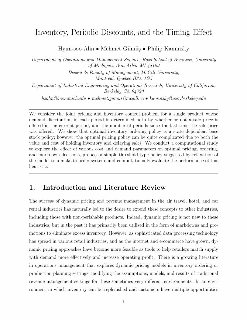
Inventory, Periodic Discounts, and the Timing Effect

Hyun-soo Ahn • Mehmet Gumus • Philip Kaminsky

Department of Operations and Management Science, Ross School of Business, Universityof Michigan, Ann Arbor MI 48109

Desautels Faculty of Management, McGill University,Montreal, Quebec H3A 1G5

Department of Industrial Engineering and Operations Research, University of California,Berkeley CA 94720

hsahn@bus.umich.edu • mehmet.gumus@mcgill.ca • kaminsky@ieor.berkeley.edu

We consider the joint pricing and inventory control problem for a single product whosedemand distribution in each period is determined both by whether or not a sale price isoffered in the current period, and the number of periods since the last time the sale pricewas offered. We show that optimal inventory ordering policy is a state dependent basestock policy; however, the optimal pricing policy can be quite complicated due to both thevalue and cost of holding inventory and delaying sales. We conduct a computational studyto explore the effect of various cost and demand parameters on optimal pricing, ordering,and markdown decisions, propose a simple threshold type policy suggested by relaxation ofthe model to a make-to-order system, and computationally evaluate the performance of thisheuristic.

1. Introduction and Literature Review

The success of dynamic pricing and revenue management in the air travel, hotel, and car

rental industries has naturally led to the desire to extend these concepts to other industries,

including those with non-perishable products. Indeed, dynamic pricing is not new to these

industries, but in the past it has primarily been utilized in the form of markdowns and pro-

motions to eliminate excess inventory. However, as sophisticated data processing technology

has spread in various retail industries, and as the internet and e-commerce have grown, dy-

namic pricing approaches have become more feasible as tools to help retailers match supply

with demand more effectively and increase operating profit. There is a growing literature

in operations management that explores dynamic pricing models in inventory ordering or

production planning settings, modifying the assumptions, models, and results of traditional

revenue management settings for these sometimes very different environments. In an envi-

ronment in which inventory can be replenished and customers have multiple opportunities

1

to buy the same product, for example, intertemporal demand interaction can significantly

impact effective ordering and pricing strategies.

In this context, intertemporal demand interaction refers to the sensitivity of current

demand not only to current pricing, but also to past pricing decisions. A quick review of the

circulars in the Sunday paper suggests that retailers use price reductions for more than just

eliminating excess inventory of out-of-season products – these retailers are instead attempting

to benefit from intertemporal demand interactions in order to increase profits. Indeed, in

a recent empirical study, Pesendorfer (2002) analyzed pricing data for selected products in

a supermarket chain, where prices were changed weekly. He used the scanner data from

three ketchup products, and observed several intertemporal price effects that drive demand

in each period. The level effect refers to the effect of the previous week’s price on the

current week’s demand. For a given current price, the current demand will be stochastically

higher when the previous week’s price was high than when the previous week’s price was low.

For a product that is periodically put on sale, the timing effect refers to the observation

that the demand at a given sale price is stochastically increasing in the time since the last

sale. Ahn et al. (2007) explore the level effect; in this paper, we explore the timing effect.

Other marketing researchers as well as economists have modeled similar issues; however,

most of this literature has focused on the effects of intertemporal demand interactions on

pricing decisions ignoring inventory considerations. Also, demand is primarily deterministic

in these models. Conlisk et al. (1984) and Sobel (1984, 1991) consider two kinds of customers

who differ in their valuation for a product. With this demand model, they show that firms

engage in cyclic pricing behavior as a traditional skimming strategy in order to distinguish

between high and low valuation customers. Assuncao and Meyer (1993) consider stockpiling

behavior of consumers who are uncertain about future prices, and investigate how frequency

of price reductions affects consumers’ purchase decision. Their analysis suggests that, as

in our model, sales volume during promotional periods is larger than sales volume during

regular periods. Slade (1998,1999) proposes a demand model in which consumers’ goodwill

increases (decreases) as the firm continues charging low (high) prices, and analyzes the

resulting optimal pricing strategy.

However, for a dynamic pricing strategy to be effective in practice, it typically has to be

aligned with inventory ordering decisions, and there are several growing streams of research

focusing on joint pricing and inventory ordering models in the operations management lit-

erature. The first stream focuses on the coordination of pricing and production decisions

2

for perishable or seasonal goods – this is typically referred to as revenue management. For

these products, it is reasonable to assume that no replenishment (production) is allowed

after the initial period, and thus most existing work focuses on analyzing the trajectory of

the optimal pricing policy as a function of remaining inventory and time. Gallego and van

Ryzin (1994) and Bitran and Mondschein (1997) consider a finite horizon dynamic pricing

problem with uncertain demand and show that the optimal price increases in the number of

periods remaining and decreases in inventory level. Subrahmanyan and Shoemaker (1996)

consider a similar problem, but allow the retailer to determine the initial stocking quan-

tity. Review papers by McGill and van Ryzin (1999), Petruzzi and Dada (1999) and Bitran

and Caldentey (2003) provide comprehensive surveys of the area. Although there are a few

recent papers that deal with more sophisticated consumer behavior (e.g., Aviv and Pazgal

(2007), Elmaghraby et al. (2007), Su (2007), and Zhou et al. (2007)), all of them assume

no replenishment during the selling season, and thus do not consider inventory/production

factors.

In the second stream, researchers consider the coordination of pricing and inventory

control with independent demand. In this stream of research, demand is a random variable

that depends only on current price. Under the assumption that unsatisfied demand in

each period is fully backlogged, Federgruen and Heching (1999) and Chen and Simchi-Levi

(2004a, 2004b) consider periodic review models with both finite and infinite horizons and

characterize the form of optimal inventory ordering policies. Polatoglu and Sahin (2000),

Chen et al. (2006) and Song et al. (2007) analyze various lost sales models. For continuous

review models, Feng and Chen (2003) model demand using a Poisson process with price-

sensitive intensity, while Chen et al. (2007) model the demand process as a Brownian

motion with price sensitive drift rate. Researchers have also explored the coordination of

pricing and inventory control with Markovian demand, where demand is a random variable

that depends on both the pricing decision and the state of the world. Gayon et al. (2007)

consider a demand model that is generated by a Markov modulated Poisson process and

obtain structural results for the optimal pricing and inventory ordering policies. Yin and

Rajaram (2007) extend Chen and Simchi-Levi’s model to the Markovian demand case and

characterize the form of the optimal policy. Several review papers provide comprehensive

surveys of research milestones and future opportunities for joint production-pricing problems;

see Eliashberg and Steinberg (1993) for classical models and Elmaghraby and Keskinocak

(2003), Yano and Gilbert (2003), Chan et al. (2004), and the references therein for recent

3

developments in this area. In most of these models, however, the current demand (or demand

intensity) is assumed to be independent of price history.

In contrast to this research, we explicitly model the relationship between current demand

and price history. In this respect, our model is most closely related to Cheng and Sethi

(1999), who consider an (endogenous) Markovian demand model where the current demand

is influenced by a state variable, which in turn is controlled by the pricing decision. However,

in our model, the demand distribution is a function of the state variable and the current

price, whereas in Cheng and Sethi (1999), the demand distribution is solely determined by

the state variable. This distinction allows us to capture the timing effect discussed above.

This paper is also related to Ahn et al. (2007), in which the authors analyze the level effect

of intertemporal demand interaction in a deterministic setting. In this paper, in contrast, we

focus on capturing the timing effect in a stochastic setting. See Gumus (2007) for a detailed

comparison of the models in Ahn et al. (2007) and those in this paper.

In this paper, we present a stylized model that captures the impact of pricing decisions

in one period on demands in others, and characterize the optimal inventory policy under

this demand model. In particular, we explicitly capture the impact of the time since the

last time a sale price was offered on the demand at a given sale price. We show that that

the presence of inventory has a non-trivial effects on dynamic pricing decisions. To develop

insight into these effects, we analyze a make-to-order version of our model, and building on

this analysis, we propose a simple threshold-type policy for the pricing strategy. Finally, we

conduct an extensive computational study to illustrate the impact of various cost and demand

parameters on pricing and inventory ordering decisions and to evaluate the performance of

our proposed threshold policy.

In the next section, we introduce our model, in which the distribution of demand in sale

periods depends on both the current price and the price history.

2. Model Formulation

We consider a discrete time, T -period finite horizon, single item stochastic demand model

where at each period the retailer offers one of two possible prices, a regular price or a sale

price, denoted pr and ps (pr > ps), respectively. At the start of each period (t = 1, . . . , T ),

the retailer makes inventory ordering (i.e., how much to order) and pricing decisions (sale or

regular) based on the current inventory level and the number of periods since the last sale.

4

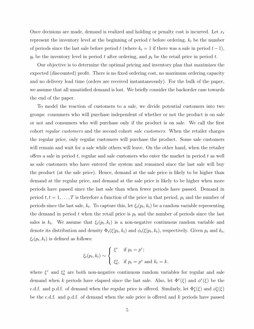
Once decisions are made, demand is realized and holding or penalty cost is incurred. Let xt

represent the inventory level at the beginning of period t before ordering, kt be the number

of periods since the last sale before period t (where kt = 1 if there was a sale in period t−1),

yt be the inventory level in period t after ordering, and pt be the retail price in period t.

Our objective is to determine the optimal pricing and inventory plan that maximizes the

expected (discounted) profit. There is no fixed ordering cost, no maximum ordering capacity

and no delivery lead time (orders are received instantaneously). For the bulk of the paper,

we assume that all unsatisfied demand is lost. We briefly consider the backorder case towards

the end of the paper.

To model the reaction of customers to a sale, we divide potential customers into two

groups: consumers who will purchase independent of whether or not the product is on sale

or not and consumers who will purchase only if the product is on sale. We call the first

cohort regular customers and the second cohort sale customers. When the retailer charges

the regular price, only regular customers will purchase the product. Some sale customers

will remain and wait for a sale while others will leave. On the other hand, when the retailer

offers a sale in period t, regular and sale customers who enter the market in period t as well

as sale customers who have entered the system and remained since the last sale will buy

the product (at the sale price). Hence, demand at the sale price is likely to be higher than

demand at the regular price, and demand at the sale price is likely to be higher when more

periods have passed since the last sale than when fewer periods have passed. Demand in

period t, t = 1, . . . , T is therefore a function of the price in that period, pt and the number of

periods since the last sale, kt. To capture this, let ξt(pt, kt) be a random variable representing

the demand in period t when the retail price is pt and the number of periods since the last

sales is kt. We assume that ξt(pt, kt) is a non-negative continuous random variable and

denote its distribution and density Φt(ξ|pt, kt) and φt(ξ|pt, kt), respectively. Given pt and kt,

ξt(pt, kt) is defined as follows:

ξt(pt, kt) ∼

ξr if pt = pr;

ξsk, if pt = ps and kt = k.

where ξr and ξsk are both non-negative continuous random variables for regular and sale

demand when k periods have elapsed since the last sale. Also, let Φr(ξ) and φr(ξ) be the

c.d.f. and p.d.f. of demand when the regular price is offered. Similarly, let Φsk(ξ) and φs

k(ξ)

be the c.d.f. and p.d.f. of demand when the sale price is offered and k periods have passed

5

since the last sale. Let µr = E[ξr] and µsk = E[ξs

k].

To capture the consumer behavior discussed above, we make the following assumption.

Assumption 1. ξr ≤ST ξs1 and ξs

k is stochastically increasing in k.

Although one could argue that regular demand should be also be effected by the frequency

of sales, we do not model this possibility in order to keep the model tractable while still

capturing relevant intertemporal demand effects.

Consider the state transitions in this lost sales model. For each period t = 1, . . . , T ,

suppose (xt, kt) represent the inventory level at the start of period t and the number of

periods since the last sale. If the retailer orders yt − xt units and sets its retail price at pt,

then the inventory level and the number of periods since the last sale at the start of period

t + 1 are described as follows:

xt+1 = max[yt − ξt(pt, kt), 0] = [yt − ξt(pt, kt)]+, t = 1, . . . , T and

kt+1 =

{kt + 1, if pt = pr;1, if pt = ps.

Throughout the paper, we define [u]+ = max[u, 0] and [u]− = max[−u, 0] for any real

number u. For a given state (xt, kt) and retailer action (yt, pt), the retailer realizes the

following revenue and costs.

• pt min[yt, ξt(pt, kt)] is the revenue in period t.

• c(yt− xt) = c · (yt− xt) is the cost of raising inventory from xt to yt in period t, where

c is the variable cost.

• h(yt − ξt(pt, kt)) = h+ · [yt − ξt(pt, kt)]+ + h− · [yt − ξt(pt, kt)]

− is the inventory and

penalty cost at the end of period t, where h+ is the per-unit holding cost and h− is

the per-unit stock-out penalty cost. Note that since we are already capturing the loss

of revenue in our revenue term, h− represents the loss of goodwill cost or any other

lost-sales related cost that is not directly related to the current revenue. (When we

consider the backorder case, the same cost function applies except that h− represents

the per-unit backorder cost.)

• fT+1(xT+1) = c · xT+1 is the salvage value function for the terminal inventory. This

is a standard assumption in many inventory finite horizon inventory models (see, e.g.,

Porteus (2002)) that will facilitate subsequent analysis.

6

Let Vt(xt, kt) be the expected discounted profit-to-go function under the optimal policy

starting from state (xt, kt) and Jt(yt, pt; xt, kt) be the expected profit-to-go function if the

retailer chooses to offer price pt and raise the inventory to level yt, and then continues

optimally afterwards. Then, the retailer’s problem can be expressed as a stochastic dynamic

program satisfying the following recursive relation:

Vt(xt, kt) = maxpt∈{pr,ps}

{maxyt≥xt

Jt(yt, pt; xt, kt)

}and

Jt(yt, pt; xt, kt) = −c(yt − xt) +

∫ ∞

0

[pt min[yt, ξ]− h+[yt − ξ]+ − h−[yt − ξ]−

+αVt+1([yt − ξ]+, kt+1)

]φt(ξ|pt, kt)dξ

where VT+1(xT+1, kT+1) = fT+1(xT+1), and α is the discount rate. For notational simplicity,

we drop time indices from decision and state variables when references are obvious.

In many inventory problems, it is useful to work with transformed versions of value

functions. We let Jt(y, p ; k) = Jt(y, p; x, k) − cx and Vt(x, k) = Vt(x, k) − cx. Then, the

optimality equations can be rewritten as follows:

Vt(x, k) = maxp∈{pr,ps}

{maxy≥x

Jt(y, p; k)

}(2.1)

where Jt(y, p; k) satisfies:

Jt(y, p ; k) =∫ ∞

0

[p min{y, ξ}− cy +αc[y− ξ]+−h+[y− ξ]+−h−[y− ξ]−+αVt+1([y− ξ]+, kt+1)]φt(ξ|p, k)dξ.

In this transformed formulation, Jt(y, p ; k) does not depend on x and the terminal

condition for the value function becomes VT+1(·) = 0. Note that we have two decision

variables and two state variables, and thus, in general the optimal decisions are functions

of the two state variables, y∗t (x, k) and p∗t (x, k). In the next section, we analyze the form

of these optimal decisions and characterize the structural relationships between the optimal

inventory ordering/pricing decisions and the state variables. In Section 4, we explore a

make-to-stock version of our model, in Section 5, we use the insight from this exploration

to develop an effective heuristic for our model and present the results of our computational

study, and in Section 6, we present several extensions of our model and conclude.

3. Optimal Policy

In order to characterize the structure of the optimal inventory ordering policy, we need to

make some additional assumptions.

7

Assumption 2. The regular and sale demand distributions (i.e., the distributions of ξr and

ξsk, k = 1, 2, . . .) are strongly unimodal.

Generally, the convolution of a unimodal distribution with a unimodal function is not

unimodal. In other words, the unimodality is not preserved by the class of unimodal dis-

tributions. Ibragimov (1965) introduced the class of strongly unimodal distributions and

defined it as follows:

Definition 1. A distribution of a random variable is said to be strongly unimodal if its

convolution with any unimodal function is unimodal.

Ibragimov (1965) proved that a strongly unimodal distribution is unimodal and showed

that the class of non-degenerate strongly unimodal distributions coincides with the class of

distributions with log-concave density. We utilize this property to show that a base stock

policy is optimal for our model. Typically, to prove the optimality of a base stock policy in

a periodic review inventory model, researchers will show that the value function is concave

(convex under minimization) in inventory order-up-to level. Since concavity of functions

is preserved under the expectation operator, an induction-based argument can be used to

demonstrate that a base stock policy is optimal for all time periods. Unfortunately, the single

period value function of this model is not concave in inventory order-up-to levels. However,

it can be shown to be unimodal, which is well known to also be a sufficient condition for the

optimality of the base stock policy, and thus we need Assumption 2 to preserve unimodality

under the expectation operator.

Although this assumption is somewhat technical, a number of important random variables

are indeed strongly unimodal. Examples include normal, truncated normal, exponential,

gamma and uniform distributions, among the others. See Dharmadhikari and Joag-Dev

(1988) for examples, results, and applications of strongly unimodal distributions.

Using this assumption, we now show that the optimal ordering policy is a state-dependent

base stock policy:

Theorem 1. Suppose that Assumption 2 holds. In each time period t, for each p and k,

there exists an optimal st(p, k) such that if the starting inventory level xt < st(p, k), it is

optimal to raise the inventory level to st(p, k), and otherwise it is optimal to do nothing.

Proof. For notational simplicity, we omit the subscripts from state and decision variables. Let kbe a positive integer and p ∈ {pr, ps}. It is sufficient to show that Jt(y, k, p) is unimodal in y for

8

given p and k. After some algebraic manipulation, we can rewrite Jt(y, p; k) as a convolution oftwo functions, the second of which is strongly unimodal by Assumption 2:

Jt(y, p; k) =∫ ∞

0Gt(y − ξ; p, k)φt(ξ|p, k)dξ

where Gt(w; p, k) is as follows:

Gt(w; p, k) = (p− c)E[ξt(p, k)]− p[w]− − (1− α)c[w]+ + c[w]− − h+[w]+ − h−[w]− + αVt+1([w]+, kt+1)

Let πt(p, k) = (p− c)E[ξt(p, k)]. Noting that E[ξt(p, k)] = µr if p = pr and that E[ξt(p, k)] = µsk

if p = ps, we have

πt(p, k) ={

(pr − c)µr, if p = pr,(ps − c)µs

k, if p = ps.

Replacing (p− c)E[ξt(p, k)] with πt(p, k) and rearranging the terms, we have

Gt(w; p, k) = πt(p, k)− (p + h− − c)[w]− − (h+ + (1− α)c)[w]+ + αVt+1([w]+, kt+1)

It is sufficient to show that for a given p and k, Gt(w; p, k) is unimodal in w since the convolutionof a unimodal function with a strongly unimodal density is also unimodal (c.f., Ibragimov (1956) orTheorem 1.10 in Dharmadhikari and Joag-Dev (1988)). We show the unimodality of Gt(w; p, k) inw by induction on t. Suppose t = T . The first term π(p, k) is constant in w. Since p + h− − c ≥ 0,the sum of the second and third terms is a unimodal function and has a unique maximizer at w = 0.Since VT+1(w, k) = cw for all w ≥ 0, we have VT+1(w, k) = 0. Hence, GT (w; p, k) is unimodal inw because the sum of functions unimodal in w that have the same unique maximizer must also beunimodal in w with the same maximizer.Now, we show that if Gt+1(w, p, k) is unimodal, Gt(w, k, p) is also unimodal. The first three termsare the same as in GT (w, p, k), and therefore the sum of these three terms is unimodal in w witha unique maximizer at w = 0. To complete the proof, we need to show that the final term (i.e.αVt+1([w]+, kt+1)) is non-increasing in w and that its maximum is achieved at w = 0. Note thatfrom induction hypothesis, Gt+1(w, p, k) is unimodal in w, so Jt+1(y, p; k) is unimodal in y. Hence,maxy≥x Jt+1(y, p; k) is non-increasing in x ≥ 0 as increasing x decreases the region over which thefunction is maximized. This implies that

Vt+1([w]+, k) = max{

maxy≥[w]+

Jt+1(y, pr; k), maxy≥[w]+

Jt(y, ps; k)}

is also non-increasing in w and achieves the maximum at w ≤ 0 since [w]+ = 0 for w ≤ 0 andVt+1([w]+, k) is the maximum of two non-increasing functions. Hence, Gt(w; p, k) is unimodal inw because the sum of functions unimodal in w that have same unique maximizer must also beunimodal in w.

Theorem 1 characterizes the optimal order quantity for a given retail price for a retailer

with starting inventory level x and k periods since the last sale. Recall that st(p, k) is the

unconstrained order-up-to level in period t when the offered price is p and the number of

periods since the last sale is k, so

st(p, k) = arg maxy≥0

Jt(y, p; k).

9

This optimal order-up-to level critically depends on two factors, the difference between the

regular and sale prices and the number of periods since the last sale. The sale demand

increases in the number of periods since the last sales, k, and this drives the desired order-

up-to level up. On the other hand, the lower retail price during the sale makes the product

less attractive and drives the order-up-to level down. Depending on which force is more

significant, the order-up-to level under the sale price can be larger (or smaller) than that

under the regular price. For many realistic scenarios, however, it is reasonable to think that

the retailer will try to sell more under the sale price than the regular price. In order to to

capture this behavior, we make the following assumption:

Assumption 3. The order-up-to level of a single period newsvendor problem with the regular

and sale price demand distributions of our model is decreasing in price. That is,

Φs(−1)1

(ps + h− − c

ps + h+ + h− − αc

)≥ Φr(−1)

(pr + h− − c

pr + h+ + h− − αc

).

Assumption 3 enables us to further characterize the structure of the optimal policy.

Theorem 2. Under Assumptions 1 - 3:

(i) When the regular price is offered, the base-stock level is independent of the number of

periods since the last sale and the number of remaining periods in the planning horizon.

That is, there exists a constant sr > 0 such that st(pr, k) = sr for all t and k.

(ii) The base-stock level under the sale price is always larger than the base-stock level under

the regular price: st(ps, k) ≥ sr for all k and t.

(iii) For a given k ≥ 1, Vt(x, k) is constant in x ∈ [0, sr] for all t.

Proof. We prove the results by induction. First, let t = T .

(i) Since VT+1(x, k) = 0 for all x ≥ 0,

JT (y, pr; k) = πT (pr, k) +∫ ∞

0

{−(p + h− − c)[y − ξ]− − (h+ + (1− α)c)[y − ξ]+}

φ(ξ|pr, k)dξ

= πT (pr, k)−∫ ∞

y(p + h− − c)(ξ − y)φ(ξ|pr, k)dξ −

∫ y

0(h+ + (1− α)c)(y − ξ)φ(ξ|pr, k)dξ

Define J′

T (y, pr; k) to be the derivative of JT (y, pr; k) with respect to y. Applying Leibniz’srule, J

′T (y, pr; k) can be written as follows:

J′

T (y, pr; k) =∫ ∞

y(pr + h− − c)φ(ξ|pr, k)dξ −

∫ y

0(h+ + (1− α)c)φ(ξ|pr, k)dξ

= (p + h− − c)− Φr(y|pr, k)(p + h+ + h− − αc)

10

where Φr(y) is the cumulative distribution of regular demand. Since JT (y, pr; k) is unimodalin y by Theorem 1, we find the maximizer (i.e. the base stock level under the regular price)employing the standard newsvendor solution:

sT (pr, k) = (Φr)−1

(pr + h− − c

pr + h+ + h− − αc

∣∣∣∣ pr, k

)

where (Φr)−1(·|pr, k) is the inverse function of the cumulative distribution of regular demandand pr+h−−c

pr+h++h−−αcis the critical fractile associated with regular price. Since Φr(y) does not

depend on k, sT (pr, k) is constant in k. We denote this base stock level sr.

(ii) sT (ps, k) ≥ sr immediately follows from Assumption 3 and ξr ≤st ξsk, k ≥ 1. Thus, VT+1(x, k) =

0 for all x ≥ 0.

(iii) For given p and k, JT (y, p; k) is a unimodal function in y. Furthermore, from part (ii)

sr = arg maxy≥0

JT (y, pr; k) ≤ arg maxy≥0

JT (y, ps; k) = sT (ps, k) for all k ≥ 1.

Hence, for any x ≤ sr,

VT (x, k) = maxp∈{pr,ps}

{maxy≥x

JT (y, p; k)}

= max[JT (sr, pr; k), JT (sT (ps, k), ps; k)

]

Therefore, VT (x, k) is a constant for x ≤ sr. On the other hand, for x > sr, we have

VT (x, k) = max[JT (x, pr; k), JT (max[x, sT (ps, k)], ps; k)

]

Since both JT (x, pr; k) and JT (max[x, sT (ps, k)], ps; k) are continuous and non-increasing inx, VT (x, k) is also continuous and non-increasing in x.

Now, assume the results hold for t + 1. We prove that they hold for t:

(i) Since Jt(y, pr; k) is unimodal in y, it is sufficient to show that sr satisfies the first ordercondition. From the induction hypothesis, Vt+1(x; k) is constant for x ≤ sr and non-increasingbeyond sr. Hence V

′t+1(x; k) = 0 for x ≤ sr. Taking the derivative of Jt(y, pr; k) with respect

to y yieldsJ

′t (y, pr; k) = (p + h− − c)− Φr(y)(p + h+ + h− − αc)

for y ≤ sr. Solving for y, we have

st(pr, k) = sr = (Φr)−1

(pr + h− − c

pr + h+ + h− − αc

∣∣∣∣ pr, k

)for all k.

From the induction hypothesis and the fact that Jt(y, pr; k) is unimodal in y, Jt(y, pr; k)achieves the maximum at y = sr.

(ii) Note that for any y ≤ sr, w = [y − ξ(p, k)]+ ≤ sr. Thus, Vt+1(w, k) remains constant for allw ≤ sr and

J′

t (y, ps; k) = (ps + h− − c)− Φsk(y)(ps + h+ + h− − αc) for y ≤ sr.

11

From Assumption 3 and the fact that ξr ≤st ξsk,

J′

t (y, ps; k)∣∣∣y=sr

= (ps + h− − c)− Φsk(s

r)(ps + h+ + h− − αc)

≥ (pr + h− − c)− Φr(sr)(pr + h+ + h− − αc) = J′

T (y, pr; k)∣∣∣y=sr

= 0.

Therefore, st(ps; k) must be greater than or equal to sr for all k.

(iii) Since sr ≤ st(ps, k), the result follows from the same argument employed when t = T .

By combining the results of previous two theorems, we can begin to characterize the

optimal pricing and inventory policy. For this purpose, in addition to the regular base stock

and sale base stock levels, we define a third critical level st(k) that represents the smallest

starting inventory level such that offering the sale price is optimal when k periods have passed

since the last sale. In other words, if the starting inventory level is below st(k), it is optimal to

charge the regular price. Note that st(k) can range from zero if offering the sale price is more

profitable for any starting inventory level (i.e., maxy≥0 JT (y, pr; k) ≤ maxy≥0 JT (y, ps; k)), to

a value greater than the regular or sale price base stock level. The structure of optimal

policy depends on the relative ordering of st(k) with respect to sr and st(ps, k):

Theorem 3. Suppose Assumptions 1 − 3 hold. If there have been k periods since the last

sale, the optimal pricing and inventory policy in period t takes one of the following three

forms depending on the starting inventory level at the beginning of period t, x, relative to the

threshold st(k):

(i) st(k) = 0 : If x ≤ st(ps, k), it is optimal to order up to st(p

s, k) and offer the sale

price ps. Otherwise, it is optimal to not order and charge a state dependent price,

p∗t (x, k) = arg maxp∈{pr,ps} Jt(x, p; k) (see Figure 1).

(ii) sr < st(k) ≤ st(ps, k): If x ∈ [0, sr), it is optimal to order up to sr and sell at the

regular price pr. If x ∈ [sr, st(k)), it is optimal not to order, and to sell the product at

the regular price pr. If x ∈ [st(k), st(ps, k)), it is optimal to order up to st(p

s, k) and

sell at the sale price ps. If x ≥ st(ps, k), it is optimal to not order, and to follow the

state dependent pricing policy, p∗t (x, k) = arg maxp∈{pr,ps} Jt(x, p; k) (see Figure 2).

(iii) st(ps, k) ≤ st(k): If x ≤ sr, it is optimal to order up to sr and sell at the regular

price pr. If x > sr, it is optimal to not order and to offer the regular price pr for

12

x ∈ (sr, st(k)), and the state-dependent price p∗t (x, k) = arg maxp∈{pr,ps} Jt(x, p; k) if

xt ≥ st(k) (see Figure 3).

Proof. Notice that from equation (2.1),

Vt(x, k) = max{

maxy≥x

Jt(y, pr; k),maxy≥x

Jt(y, pr; k)}

.

Define J∗t (x, pr; k) = maxy≥x Jt(y, pr; k) and J∗t (x, ps; k) = maxy≥x Jt(y, ps; k), respectively. Bothare non-increasing in x by Theorem 1. Specifically, from Theorems 1 and 2, J∗t (x, pr; k) =Jt(sr, pr; k) for x ≤ sr and J∗t (x, pr; k) = Jt(x, pr; k) otherwise, and J∗t (x, ps; k) = Jt(st(ps; k), ps; k)for x ≤ st(ps; k) and J∗t (x, pr; k) = Jt(x, pr; k) otherwise. Hence, the structure of the optimal policyis determined by how these two non-increasing functions behave with respect to starting inventorylevel x; we explore three different cases:

Case 1: Jt(sr, pr; k) ≤ Jt(st(ps; k), ps; k)The fact that st(ps; k) ≥ sr (Theorem 2.(ii)) and the fact that Jt(y, p; k) is unimodal in yimply that

J∗t (x, pr; k) = Jt(sr, pr; k) ≤ J∗t (x, ps; k) = Jt(st(ps; k), ps; k) for x ≤ sr and,

J∗t (x, pr; k) ≤ Jt(sr, pr; k) ≤ J∗t (x, ps; k) = Jt(st(ps; k), ps; k) for sr < x ≤ st(ps; k).

Hence, as long as the starting inventory x is below st(ps; k), it is optimal to raise theinventory level to st(ps; k) and offer the sale, hence st(k) = 0. For x > st(ps; k), no-tice that the unimodality of Jt(y, p; k) in y implies that J∗t (x, pr; k) = Jt(x, pr; k) andJ∗t (x, ps; k) = Jt(x, ps; k), thus it is optimal to charge a state-dependent price p∗t (x, k) =arg maxp∈{pr,ps} Jt(x, p; k) and not order.

Case 2: Jt(sr, pr; k) > Jt(st(ps; k), ps; k) and Jt(st(ps; k), pr; k) ≤ Jt(st(ps; k), ps; k)Applying the condition and using the fact that st(ps; k) ≥ sr, we have

J∗t (x, pr; k) = Jt(sr, pr; k) > J∗t (x, ps; k) = J∗t (st(ps; k), ps; k) for x ≤ sr.

For x ≤ sr, ordering up to sr and selling at the regular price pr is therefore optimal.

For x ∈ (sr, st(ps; k)], note that J∗t (x, pr; k) = Jt(x, pr; k), which is (weakly) decreasing whileJ∗t (x, ps; k) remains to be J t(st(ps; k), ps; k). Since Jt(y, pr; k) is continuous in y, there mustbe a st(k) ∈ (sr, st(ps; k)] such that

st(k) = min{x ∈ (sr, st(ps; k)] | Jt(x, pr; k) = J∗t (st(ps; k), ps; k)}.

It follows from the definition of st(k) and the unimodality of Jt(y, pr; k) that

J∗t (x, pr; k) = Jt(x, pr; k) > Jt(st(ps; k), ps; k) for sr ≤ x < st(k) and

J∗t (x, pr; k) = Jt(x, pr; k) ≤ J∗t (x, ps; k) = J∗t (st(ps; k), ps; k) for st(k) ≤ x ≤ st(ps; k).

Hence, when sr ≤ x < st(k), it is optimal to sell the existing inventory at the regular price,pr and not order. On the other hand, if st(k) ≤ x ≤ st(x, k), then it is optimal to raisethe inventory to st(x, k) and sell at the sale price, ps. For x > st(ps; k), J∗t (x, pr; k) =Jt(x, pr; k) and J∗t (x, ps; k) = Jt(x, ps; k). Hence, it is optimal to follow a state-dependentprice p∗t (x, k) = arg maxp∈{pr,ps} Jt(x, p; k) and not order.

13

Case 3: Jt(sr, pr; k) ≥ Jt(st(ps; k), pr; k) > Jt(st(ps; k), ps; k).Applying the inequality Jt(sr, pr; k) > Jt(st(ps; k), ps; k) and the fact that st(ps; k) ≥ sr againimply that

J∗t (x, pr; k) = Jt(sr, pr; k) > J∗t (x, ps; k) = J∗t (st(ps; k), ps; k) for x ≤ sr.

For x ≤ sr, ordering up to sr and selling at the regular price pr is therefore optimal. Noticethat the condition implies that

Jt(sr, pr; k) ≥ J∗t (x, pr; k) = Jt(x, pr; k) > Jt(st(ps; k), ps; k) for x ∈ (sr, st(ps, k),

so it is optimal to sell the existing inventory at the regular price, pr, and not order. Ifx > st(ps, k), then it is optimal to not order in either price. Hence, it is optimal to follow astate-dependent price p∗t (x, k) = arg maxp∈{pr,ps} Jt(x, p; k) and not order.

Ordering Policy

Pricing Policyps ps p∗t (xt, kt)

st(kt) = 0 sr st(ps, kt)

st(kt) = 0 sr st(ps, kt)

xt

xt

Figure 1: Optimal base stock and pricing policy when st(k) = 0

Ordering Policy

Pricing Policy

0

p∗t (xt, kt)

st(ps, kt)

st(ps, kt)

xt

xtpspr pr

st(kt)

st(kt)sr

sr

0

Figure 2: Optimal base stock and pricing policy when st(k) ∈ [sr, st(p, k))

Ordering Policy

Pricing Policy

0

p∗t (xt, kt)

xt

xtpr pr

sr

sr

st(kt)

st(kt)

pr

st(ps, kt)

st(ps, kt)0

Figure 3: Optimal base stock and pricing policy when st(k) ∈ [st(p, k),∞]

In general, when the starting inventory level is higher than the appropriate base stock

level (regular or sale base stock as described above), the optimal pricing policy becomes state

14

dependent. In fact, the optimal pricing policy can be quite complicated with respect to both

state variables, as we illustrate with several examples.

First, consider the change in p∗t (x, k) with respect to x for a fixed k. Intuitively, one

might expect that p∗t (x, k) would decrease in starting inventory x because higher starting

inventory level lead to higher inventory holding costs, suggesting that inventory should be

liquidated through a sale. However, this intuition is not in general correct. To see this,

consider the following simple 2-period example with the following demand function:

Example 1.

ξt(p, k) =

{[12 + εr]

+ , if p = pr;[∑ki=1 18(1− β)i−1 + εs

]+

, if p = ps.

where β = 0.1 and εr and εs are normally distributed random variables with E[εr] = E[εs] = 0,

σεr = 4 and σεs = 6. Finally, pr = 30, ps = 15, h+ = 4, h− = 0, c = 10, α = 1 and the

planning horizon is T = 2 periods long.

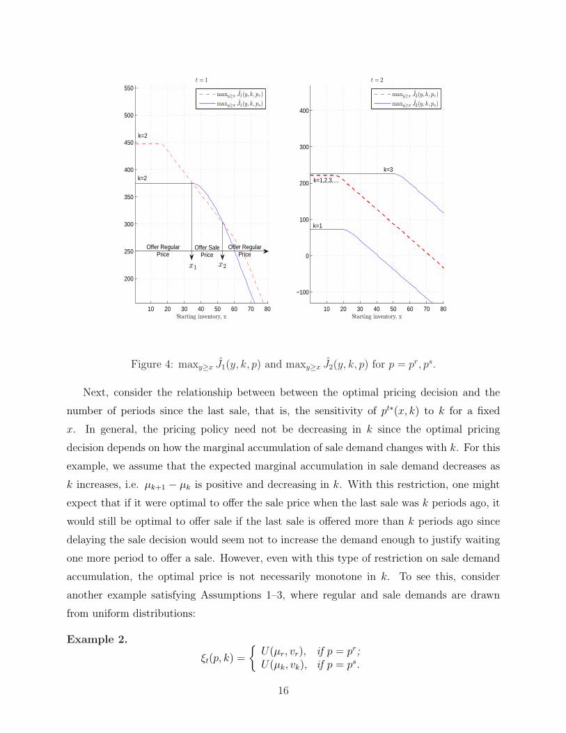
It can be shown that Example 1 satisfies Assumptions 1-3. Figure 4 plots maxy≥x Jt(y, k, pr)

and maxy≥x Jt(y, k, ps) with respect to x for k = 2 in period one, and for k = 1 and k = 3

in period two. Recall that the optimal pricing decision at period t is determined by the

point-wise maximization of maxy≥x Jt(y, k, pr) and maxy≥x Jt(y, k, ps):

p∗t (x, k) = arg maxp∈{pr,ps}

{maxy≥x

Jt(y, k, p)}

and that if k = 2 in period one, it will either equal 1 or 3 in period two. Observe that in

period one (the left graph) the plots of maxy≥x J1(y, 2, pr) and maxy≥x J1(y, 2, ps) cross each

other both at point x1 and point x2, implying that the optimal pricing decision at in period

one first switches from regular to sale price at x1 and then back to regular price at x2 as

starting inventory increases. Why is this the case?

From Figure 4, observe that of the four possible pricing strategies, two dominate. Offer

regular price in the first period and sale price (call this strategy-RS) and offer sale price

in the first period and regular price in the second (strategy-SR). When initial inventory

is low, RS dominates, but as initial inventory increases, the leftover inventory and thus

holding cost in period one begins to increase, until SR becomes preferable. However, as

starting inventory continues to increase, at some point the leftover inventory at the end of

period two becomes significant, and so RS again dominates, since it eliminates additional

inventory in period two.

15

10 20 30 40 50 60 70 80

200

250

300

350

400

450

500

550t = 1

Starting inventory, x

maxy≥x J1(y, k, pr)

maxy≥x J1(y, k, ps)

10 20 30 40 50 60 70 80

−100

0

100

200

300

400

t = 2

Starting inventory, x

maxy≥x J2(y, k, pr)

maxy≥x J2(y, k, ps)

x1x2

k=2

k=2

k=1

k=1,2,3,…

k=3

Offer RegularPrice

Offer SalePrice

Offer RegularPrice

Figure 4: maxy≥x J1(y, k, p) and maxy≥x J2(y, k, p) for p = pr, ps.

Next, consider the relationship between between the optimal pricing decision and the

number of periods since the last sale, that is, the sensitivity of pt∗(x, k) to k for a fixed

x. In general, the pricing policy need not be decreasing in k since the optimal pricing

decision depends on how the marginal accumulation of sale demand changes with k. For this

example, we assume that the expected marginal accumulation in sale demand decreases as

k increases, i.e. µk+1 − µk is positive and decreasing in k. With this restriction, one might

expect that if it were optimal to offer the sale price when the last sale was k periods ago, it

would still be optimal to offer sale if the last sale is offered more than k periods ago since

delaying the sale decision would seem not to increase the demand enough to justify waiting

one more period to offer a sale. However, even with this type of restriction on sale demand

accumulation, the optimal price is not necessarily monotone in k. To see this, consider

another example satisfying Assumptions 1–3, where regular and sale demands are drawn

from uniform distributions:

Example 2.

ξt(p, k) =

{U(µr, vr), if p = pr;U(µk, vk), if p = ps.

16

where U(µ, v) is a uniform random variable that has a support from µ − v to µ + v. Let

µr = 6, vr = 3, µk = 9∑k

i=1 βi−1 and vk = vr

√∑ki=1 β2(i−1) with β = 0.90. Finally, pr = 30,

ps = 15, h+ = 5, h− = 0, c = 10, α = 1 and the planning horizon is T = 2 periods.

10 15 20 25

160

180

200

220

240

260

280

300

320

340

t = 1

Starting inventory, x

maxy≥x J1(y, k, pr)

maxy≥x J1(y, k, ps)

0 10 20 30 40 50 60 70

−200

−100

0

100

200

300

t = 2

Starting inventory, x

maxy≥x J2(y, k, pr)

maxy≥x J2(y, k, ps)

x1

x2

k=3

k=3

k=4

k=4

k=4

k=5

k=1

k=1,2,3,…

Offer RegularPrice

Offer RegularPrice

Offer SalePrice

Offer SalePrice

Figure 5: maxy≥x J1(y, k, p) and maxy≥x J2(y, k, p) for p = pr, ps.

As for the previous example, we illustrate the possible strategies in figure 5, and as before,

of the four possible pricing strategies, two dominate. Offer regular price in the first period

and sale price (strategy-RS) and offer sale price in the first period and regular price in the

second (strategy-SR). Observe that in period two, for any starting inventory between x1

and x2, for k = 4 RS dominates, but for k = 3, SR dominates. Again, this counterintuitive

behavior is caused by two opposite effects. On one hand, as k increases from 3 to 4, the

total demand over two periods doesn’t change much regardless of whether RS or SR is

employed due to the nature of the demand function. On the other hand, RS generates

leftover inventory that lasts two periods rather than one, which impacts the overall cost

more as k increases from 3 to 4.

In both these examples, the future impact of current inventory (we call this the long-term

or propagation effect) has a direct and somewhat counterintuitive impact on optimal policy.

17

4. The Make-to-order System

As we demonstrated in the previous section, the optimal policy of our model is sometimes

quite complicated, as pricing and inventory decisions are influenced by intertemporal de-

mand, starting inventory level, and the remaining planning horizon. In general, the optimal

pricing policy is not necessarily monotone in starting inventory level or time since the last

sale. In order to isolate the intertemporal demand effect on the pricing component of our

model, we next consider a simplified version of the model, in which we assume that the

retailer places an order after it sees the realized demand- a “make-to-order” system that is,

from the perspective of the retailer, deterministic. In this case, it is optimal to order exactly

the realized demand, thus the state is simply k, the number of periods since the last sale.

We write the retailer’s problem as a deterministic dynamic programming problem:

Vt(kt) = maxpt∈{pr,ps}

[π(pt, kt) + αVt+1(kt+1)]

where π(pt, kt) = (pr− c)µr if pt = pr; (ps−c)µsk if pt = ps, and VT+1(k) = 0 for all k. Noting

that the demand at the regular price is independent of the the number of periods since last

sale , we omit k in π(pr, k) and write it as π(pr).

We assume that the expected demand under the sale price, E[ξ(ps, k)] = µsk is strictly

concave and increasing in k, that is, µsk+1 − µs

k > µsk+2 − µs

k+1 ≥ 0, so that the marginal

accumulation of sale demand decreases as k increases. Under this assumption, we show that

a threshold policy is indeed optimal: there is a k∗t such that it is optimal to charge the

regular price, pr, if k ≤ k∗t , and to offer the sale price ps, otherwise.

Theorem 4. Let p∗t (k) be the optimal price at period t when k periods have passed since the

last sale. Then,

(i) p∗t (k) is non-increasing in k.

(ii) Vt(k + 1)− Vt(k) ≤ π(ps, k + 1)− π(ps, k) for all k = 1, . . . , t and t = 1, . . . , T .

In Appendix A, we prove this result by induction.

For finite horizon problems, finding the optimal pricing policy is quite straight forward, as

one can recast the dynamic programming as a shortest path problem. Indeed, this motivates

us to explore the effectiveness of this type of threshold policy for our original model, the

make-to-order model. We investigate this in the computational section of the paper.

18

4.1 The Infinite Horizon Model

The threshold levels suggested by Theorem 4 are in general time dependent, so that there

exists k∗t for each period t such that if the number of periods since the last sale is less than

k∗t , it is optimal to offer regular price and otherwise it is optimal offer sale price. In order to

better understand the nature of these threshold levels, we next consider the infinite horizon

version of this problem in both the discounted and average profit cases.

For both cases, in Appendix B, we prove that time invariant optimal threshold levels, k∗

exist for each period t. In other words,

Lemma 1. There exists an optimal stationary policy for both discounted and average profit

cases.

This suggests that there exists a cyclic policy where offering a sale every k∗ periods is

optimal. In order to characterize the optimal cycle length (that is, the optimal stationary

threshold level), we write the expected profit associated with a policy in which the sale price

is offered every k periods and find the optimal cycle length. Let Πα(k) and ΠA(k) be the

discounted and average expected profit of a k-period cyclic policy with initial state k0 = 1,

respectively. After some algebraic manipulation, we get, for all k ≥ 1,

Πα(k) =π(pr)

1− α+ αk−1π(ps, k)− π(pr)

1− αk(Discounted profit), and

ΠA(k) = π(pr) +π(ps, k)− π(pr)

k(Average profit).

The derivations of both expressions above are delegated to the Appendix C. From this, it

is easy to see that a periodic sale is better than selling at regular price every period if and

only if there exists a k such that π(ps, k)− π(pr) ≥ 0. In such case, the optimal cycle length

is the one that maximizes the profit:

kα∗ = arg max[αk−1π(ps, k)− π(pr)

1− αk] (Discounted profit), and

kA∗ = arg maxπ(ps, k)− π(pr)

k(Average profit).

To find the optimal cycle length, it suffices to consider k ≥ k = min{k|π(ps, k)−π(pr) ≥0}.

Lemma 2. In the infinite horizon discounted profit problem with discount factor α, for

k ≥ k,

19

(i) the k-period cyclic policy is better than the k + 1-period cyclic policy if and only if

π(ps, k + 1)− π(ps, k)

π(ps, k)− π(pr)≤ 1/α∑k

i=1 αi−1=

1− α

α

1

1− αk(4.1)

(ii) Πα(k) is unimodal in k.

Lemma 3. In the infinite horizon average profit problem, for k ≥ k,

(i) The k-period cyclic policy is better than a k + 1-period cyclic policy if and only if

π(ps, k + 1)− π(ps, k)

π(ps, k)− π(pr)≤ 1

k(4.2)

(ii) ΠA(k) is unimodal in k .

The proofs of of these lemmas are in Appendices D and E. Conditions (4.1) and (4.2)

imply that if the marginal benefit of extending the cycle by one period becomes sufficiently

small, then it is optimal to not extend the length of a cycle. In fact, both conditions describe

precisely the minimum marginal gain required to optimally extend the cycle length by at

least one period. Solving for the optimal cycle length is not hard since, in both cases, the

profit function is unimodal in k.

We employ Lemmas 2 and 3 to characterize the optimal pricing policy for the infinite

horizon problem.

Theorem 5. In the discounted profit problem,

(i) It is optimal to sell at the regular price in every period if and only if π(pr) ≥ π(ps, k)

for all k ≥ 1.

(ii) Otherwise, it is optimal to use the k∗-period cyclic pricing policy where k∗ is the small-

est integer greater than k satisfying condition (4.1).

The same results hold for the average profit case with condition (4.2) replacing condition

(4.1).

The proof can be found in Appendix D (discounted profit case) and Appendix E (average

profit case).

This result is related to other intertemporal pricing results, such as those in Sobel (1984)

and Pesendorfer (2002). Both papers model the demand accumulation assuming customers

20

are strategic and characterize the equilibrium pricing policy that consists of periodic price

reductions. In contrast to their models, this paper considers more general demand accumu-

lations and fully characterizes the optimal pricing policies for both discounted and average

profit cases with myopic customers. This result is also qualitatively similar to the optimality

of 2-period cyclic pricing policy proved in Ahn et al. (2007) where customers stay in the

market for at most 2 periods.

5. Computational Studies

We completed two computational studies, one to assess the impact of system parameters on

the operation of the system, and one to assess the the performance of a simple threshold

policy for this system in light of the potentially complicated structure of the optimal policy

discussed previously.

5.1 The Operational Impact of System Parameters

In this set of experiments, we vary the system parameters described below, and assess the

impact of these parameters on the optimal number of sales over the time horizon, as well as

(for the case of markdown percentage) the impact on expected profit. The parameters we

vary can be divided into three categories:

Prices We fix the regular price, pr and vary the markdown percentage. Let δ be the

percentage markdown with respect to the regular price, i.e.

∆ =

(1− ps

pr

)100%

Production parameters We use stationary linear production costs and inventory holding

costs (where shortage cost is zero), i.e. ct(x) = cx and ht(x) = h+x+ for all t = 1, . . . T .

Furthermore, we vary the holding cost as a percentage of production cost, i.e. h =

h+

c100%, and the production cost as a percentage of regular price, i.e.

m =

(pr − c

pr

)100%

where m is the percentage markup for the regular price.

21

Demand scenarios For the demand distributions, we use truncated normal random vari-

ables. Let N+(µ, σ) be the positive part of a normal random variable with mean µ and

standard deviation σ, then:

ξt(pt, kt) =

{N+(µr, cvµ

r), if pt = pr;∑kt

i=1 N+(µsi , cvµ

si ), if pt = ps.

where cv is coefficient of variation (the ratio of the standard deviation to the mean),

µr = µ(pr) and

µsi =

{µ(ps), if i = 1;µ(ps)γ(1− β)i−1, if i > 1.

where 0 < β < 1 and 0 < γ < 1. Note that the expected marginal accumulation

of sale demand is controlled by two parameters, β and γ. β controls the decrease in

rate of expected marginal accumulation as the time since the last sale increases. For

example, if β = 0.50, then the marginal accumulation decreases by half each period

that the retailer delays the sale decision. γ controls the ratio of expected marginal

accumulation in sale demand to the sale demand in the first period after a sale.

5.1.1 One Varying Parameter

For the initial computational study, we consider a base scenario and change the various

parameters one at a time, fixing the other parameters at the base level.

Set of Parameters We consider three values for each of the parameters:

1. We fix pr = 20 and change the markdown percentage with respect to regular price

by varying ∆: {10%, 20%, 30%}.2. We assume that µ(p) = 30− p.

3. The rate of decrease in marginal accumulation in sale demand measured by β:

{0.05, 0.15, 0.25}.4. The proportion of expected marginal accumulation sale demand to expected sale

demand at k = 1 is varied by varying γ =µs

1−µr

µs1

.

5. The uncertainty in demand as measured by the coefficient of variation cv: {0.20, 0.30, 0.40}.6. Percentage markup for the regular price m: {50%, 70%, 90%}.7. Inventory holding cost as a percentage of unit cost h: {10%, 15%, 20%}.

22

Base instance We use following values for the base instance:

{∆ = 10%, β = 0.15, cv = 0.20,m = 50%, h = 10%}.

Finally, we fix the discount factor, α = 0.9.

20 40 60 80 100Initial Inventory Level, x

m = 0.5m = 0.7m = 0.9

0 20 40 60 80 1000

2

4

6

8

10

Ns(x

)

Initial Inventory Level, x

h = 0.1h = 0.15h = 0.2

20 40 60 80 100Initial Inventory Level, x

r = 0.1r = 0.2r = 0.3

0 20 40 60 80 1000

2

4

6

8

10

Ns(x

)

Initial Inventory Level, x

β = 0.15β = 0.25β = 0.05

20 40 60 80 100Initial Inventory Level, x

cv = 0.2cv = 0.3cv = 0.4

Figure 6: Plots of Ns(x) for various cases

We computationally solve the dynamic program programming problem for this study. For

each instance, we solve a 12-period problem (i.e. T = 12) and calculate the optimal decision

rules, both inventory order-up-to levels and pricing decisions, i.e. (y∗t (x, k), p∗t (x, k)). Then,

we compute the expected number of sales during the planning horizon:

Ns(x) = E[number of sales|x0 = x, k0 = 1]

where the initial inventory level is x (i.e. x0 = x) and the initial k is 1 (i.e. k0 = 1). The

results are plotted in Figure 6. Each plot shows a set of three plots of Ns(x) for different

values of a specific parameter as the rest of the parameters are held constant at the base

level. We observe the following:

23

• The expected number of sales increases as the initial inventory level increases. This

behavior can be observed in almost all plots in Figure 6. This is quite intuitive since

as inventory increases, the retailer will want to offer sale more frequently in order to

liquidate the excess inventory as quickly as possible. In a few cases (see the figure in

which the markdown percentage ∆ is varied), the expected number of sales decreases

as the inventory increases for the high inventory levels. Recall our discussion at the

end of Section 3, where we pointed out that in some instances, the firm delays its sale

decision to avoid the propagation of excess inventory and this causes expected total

number of sales to decrease when the inventory is high.

• As individual parameters vary:

– As the markup from cost for the regular price decreases, the expected number

of sales decreases for all initial inventory levels. This behavior is intuitive as

decreasing the markup also decreases the profit margins, making it necessary for

the firm to delay the sale decision in order to accumulate a profitable level of sale

demand. This in turn leads to less frequent sales.

– The expected number of sales increases for all inventory levels as the unit inventory

cost increases. This is also quite intuitive since increasing holding costs make it

costly to delay the sale decision, inducing more frequent sales.

– As the markdown percentage goes up (that is, the sale prices go down), it is

optimal to offer less frequent sales. As sale prices decrease, both sale demand and

marginal accumulation in sale demand increase. This leads to less frequent sales,

so that the firm can take advantage of larger accumulations in sale demand.

– As the speed of decrease in marginal accumulation in sale demand increases,

the expected number of sales increases. Marginal accumulation in sale demand

decreases more rapidly as β increases, and thus it becomes less and less profitable

to delay the sale decision, since waiting for an additional period to accumulate

additional sales demand does not generate enough revenue to justify the wait.

– The expected number of sales decreases as the coefficient of variation in demand

increases, but the impact is marginal.

24

1.5 2 2.5 3markdown percentage (i.e. r)

m = 0.5m = 0.7m = 0.9

1 1.5 2 2.5 31

2

3

4

5

Ns

speed of decrease in marginal accumulation (i.e. β)

m = 0.5m = 0.7m = 0.9

1.5 2 2.5 3holding cost

m = 0.5m = 0.7m = 0.9

1 1.5 2 2.5 31.5

2

2.5

3

3.5

4

Ns

speed of decrease in marginal accumulation (i.e. β)

r = 0.1r = 0.2r = 0.3

1.5 2 2.5 3holding cost

r = 0.1r = 0.2r = 0.3

1 1.5 2 2.5 31.5

2

2.5

3

3.5

4

Ns

holding cost

β = 0.05β = 0.15β = 0.25

Figure 7: Plots of expected number of sales for various cases

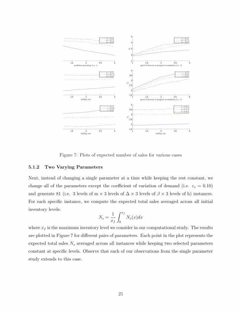
5.1.2 Two Varying Parameters

Next, instead of changing a single parameter at a time while keeping the rest constant, we

change all of the parameters except the coefficient of variation of demand (i.e. cv = 0.10)

and generate 81 (i.e. 3 levels of m × 3 levels of ∆ × 3 levels of β × 3 levels of h) instances.

For each specific instance, we compute the expected total sales averaged across all initial

inventory levels:

Ns =1

xf

∫ xf

0

Ns(x)dx

where xf is the maximum inventory level we consider in our computational study. The results

are plotted in Figure 7 for different pairs of parameters. Each point in the plot represents the

expected total sales Ns averaged across all instances while keeping two selected parameters

constant at specific levels. Observe that each of our observations from the single parameter

study extends to this case.

25

5.1.3 Varying Markdown Percentage

Recall that in our model, the markdown percentage is assumed to be constant. Next, we

analyze the impact on total profit of varying markdown percentage. For this purpose, we

compute the expected total profit for various levels of markdown percentage:

Π∗(∆) = E[Total Profit|x0 = 0, k0 = 1]

where the markdown percentage is ∆, initial inventory level is 0 (i.e. x0 = 0) and initial k

is 1 (i.e. k0 = 1). The results are plotted in Figure 8. Each plot in the figure shows a set of

three curves representing Π∗(∆) for different values of a specific parameter, while the rest of

parameters are held constant at the base level. Observe the following:

• In almost all cases, the expected total profit first increases and then decreases as

markdown percentage increases and achieves its maximum level at some markdown

percentage level.

• As a single parameter varies, we observe:

– The expected total profit increases for all markdown levels as the regular price

markup percentage increases whereas it decreases as holding cost, uncertainty

in demand and speed of decrease in marginal demand accumulation goes up. All

these results are self-explanatory except for the impact of decrease rate in marginal

demand accumulation (i.e. β). As β increases, the sale demand accumulates very

fast in the beginning, however its growth slows down later. This causes more

frequent sales and less accumulation in sale demand. This in turn decreases the

expected total profit that can be generated.

– The markdown level that maximizes the expected total profit within the range of

computational study increases as the markup percentage (that is, the markup of

from cost to regular price) goes up. This is because a relatively lower cost (that

is, higher regular price) allows the firm to decrease the sale price, generating more

profit due to both increased sale demand and increased marginal accumulation of

sale demand.

– The optimal markdown level increases as the speed of decrease in marginal de-

mand accumulation decreases. We’ve seen that the smaller β is, the less frequently

26

sales occur. As in the previous item, this induces the firm to decrease the sale

price in order to generate more revenue due to increased sale demand.

– The impact of holding cost and coefficient of variation of demand on the optimal

markdown percentage appears to be marginal.

0.15 0.2 0.25 0.3Markdown percentage

m = 0.5m = 0.6m = 0.7

0.1 0.15 0.2 0.25 0.31200

1220

1240

1260

1280

1300

Expecte

dP

rofit

Markdown percentage

h = 0.1h = 0.15h = 0.2

0.15 0.2 0.25 0.3Markdown percentage

β = 0.15β = 0.25β = 0.05

0.1 0.15 0.2 0.25 0.31180

1200

1220

1240

1260

1280

1300

Expecte

dP

rofit

Markdown percentage

cv = 0.2cv = 0.3cv = 0.4

Figure 8: Plots of expected profits with respect to markdown percentage (i.e. Delta) forvarious cases

5.2 A Threshold Heuristic

Recall that the optimal pricing policy for the make-to-stock model can be quite complicated.

Thus, we are motivated to test a simple threshold policy suggested by the make-to-order

model:

Threshold Policy

• If k < k∗t then offer regular price and use base stock with sr.

• If k ≥ k∗t then offer sale price and use base stock with s(ps, k).

27

To implement this policy, we utilize threshold levels found by solving the deterministic

dynamic programming problem for the make-to-order version of the particular instance we

are interested in. We then manage the inventory using base stock policy with the following

levels:

sr = (Φr)−1(f r)

and

s(ps, k) = (Φsk)−1(f s)

where f r and f s are the critical fractiles of the single period problem associated with regular

and sale prices, respectively. Note that the sr is equal to the optimal base stock associated

with regular price and s(ps, k) is greater than the optimal base stock level associated with

sale price st(ps, k).

Of course, the optimal cost for a particular make-to-order instance will be less than

the optimal cost of the equivalent make-to-stock instance since the former avoids inventory

costs, and thus these threshold levels come from solving a potentially very different problem.

Nevertheless, this heuristic approach seems to be a reasonable compromise between the

complexity of the actual policy, and a policy which is relatively simple to calculate and

implement.

As before, we evaluate the performance of this policy by changing a single parameter at a

time while fixing the rest of the parameters at base levels. We plot expected profits that are

generated by optimal versus threshold type policies policies as a function of initial inventory

level, x0 = x assuming k0 = 1. Now,let Π∗(x) and ΠH(x) be the expected profits generated

by optimal and heuristic policies, respectively.

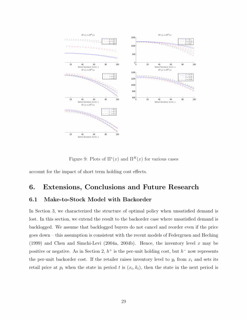
The results are plotted in Figures 9. Each plot shows a set of three plots of Π∗(x) and

ΠH(x) for different values of a specific parameter, while the rest of parameters are held

constant at the base level. We observe that in general, the heuristic policy performs quite

well. Remember that a sale is scheduled at a particular time for two reasons: to clear excess

inventory or to generate more revenue by strategically delaying the sale until expected sale

demand has accumulated. The optimal policy reflects both of these sales criteria, whereas

the heuristic policy only reflects the strategic value of delaying sale.incentives to the pricing

policy whereas the heuristic policy reflects only strategic incentive of sales decision to pricing

policy. In spite of that, heuristic policy performing quite well, particularly when inventory is

low. However, as inventory gets higher, the quality of the heuristic degrades, since it doesn’t

28

20 40 60 80 100

Π∗(x) vs ΠH(x)

Initial Inventory Level, x

0 20 40 60 80 1000

500

1000

1500Π∗(x) vs ΠH(x)

Initial Inventory Level, x

20 40 60 80 100

Π∗(x) vs ΠH(x)

Initial Inventory Level, x

0 20 40 60 80 100600

800

1000

1200

1400Π∗(x) vs ΠH(x)

Initial Inventory Level, x

20 40 60 80 100

Π∗(x) vs ΠH(x)

Initial Inventory Level, x

m = 0.5m = 0.7m = 0.9

h = 0.1h = 0.15h = 0.2

r = 0.1r = 0.2r = 0.3

β = 0.15β = 0.25β = 0.05

cv = 0.2cv = 0.3cv = 0.4

Figure 9: Plots of Π∗(x) and ΠH(x) for various cases

account for the impact of short term holding cost effects.

6. Extensions, Conclusions and Future Research

6.1 Make-to-Stock Model with Backorder

In Section 3, we characterized the structure of optimal policy when unsatisfied demand is

lost. In this section, we extend the result to the backorder case where unsatisfied demand is

backlogged. We assume that backlogged buyers do not cancel and reorder even if the price

goes down – this assumption is consistent with the recent models of Federgruen and Heching

(1999) and Chen and Simchi-Levi (2004a, 2004b). Hence, the inventory level x may be

positive or negative. As in Section 2, h+ is the per-unit holding cost, but h− now represents

the per-unit backorder cost. If the retailer raises inventory level to yt from xt and sets its

retail price at pt when the state in period t is (xt, kt), then the state in the next period is

29

described as follows:

xt+1 = yt − ξt(pt, kt), t = 1, . . . , T, and

kt+1 =

{kt + 1, if pt = pr;1, if pt = ps.

We assume that demand is fulfilled on a first-come-first-serve basis, so that no demand in

the current period will be satisfied without first clearing backorders. Just as in the lost sale

case, we subtract the ordering cost cx in each period to transform the original model into

an equivalent, but more tractable, form. As before, let Vt(x, k) be the optimal expected

discounted revenue from period t and onwards, and Jt(y, p; k) be the expected discounted

revenue of a policy that raises the inventory to y and sets the retail price p in period t and

follows the optimal policy afterward. Then,

Vt(x, k) = maxp∈{pr,ps}

{maxy≥x

Jt(y, p; k)

}

where Jt(y, p; k) satisfies:

Jt(y, p; k) =

∫ ∞

0

[pξ−cy+αc(y−ξ)−h+[y−ξ]+−h−[y−ξ]−+αVt+1(y−ξ, kt+1)]φt(ξ|p, k)dξ.

To facilitate our analysis, we make the following assumption in addition to Assumptions 1

and 2:

Assumption 4. h− > (1− α)c.

This implies that satisfying the demand in the current period is better than delaying it

for one period and satisfying it in the next period, and it is a fairly standard assumption

in the inventory literature. Furthermore, the result is trivial when Assumption 4 does not

hold: The firm simply accrues all backorders until the end of horizon. In Appendix F, we

prove that a base-stock policy is optimal when the price and number of periods since the

last sale are fixed:

Theorem 6. Suppose that Assumptions 1, 2 and 4 hold. Jt(y, p; k) is unimodal in y for given

p and k. Therefore, a base-stock policy is optimal.

Similarly, the result of Theorem 2 can be extended to the backorder case. Unlike the

lost sale case, we do not need Assumption 3, as the critical fractiles, which determine the

order-up-to levels, do not depend on the retail price. In Appendix G, we prove:

30

Theorem 7. If Assumptions 1,2, and 4 hold, then

(i) When the regular price is offered, the base-stock level is independent of the number of

periods since the last sale and the number of remaining periods in the planning horizon.

That is, there exists a constant sr > 0 such that i.e. st(pr, k) = sr for all t and k.

(ii) The base-stock level under the sale price is always larger than the base-stock level under

the regular price: st(ps, k) ≥ sr for all k and t.

(iii) For given k ≥ 1, Vt(x, k) is constant in x ∈ [0, sr] for all t.

Using Theorems 6 and 7, we now characterize the optimal pricing and inventory policy

for the backorder case. As in the lost sale case, let st(k) be the smallest starting inventory

level such that offering a sale is optimal when k periods have passed since the last sale.

Theorem 8. Suppose that Assumptions 1, 2 and 4 hold. Then, if there have been k periods

since the last sale, the optimal pricing and inventory policy in period t takes one of the

following three forms depending on the starting inventory level at the beginning of period t,

x, relative to st(k):

(i) st(k) < sr: If x ≤ st(ps, k), it is optimal to order up to st(p

s, k) and sell at the sale

price ps. Otherwise, it is optimal not to order, and to follow the state dependent pricing

policy, p∗t (x, k) = arg maxp∈{pr,ps} Jt(x, p; k).

(ii) sr ≤ st(k) < st(ps, k): If x < sr, it is optimal to order up to sr and sell at the regular

price pr. If x ∈ [sr, st(k)), it is optimal not to order, and to sell at the regular price pr.

If x ∈ [st(k), st(ps, k)), it is optimal to order up to st(p

s, k) and sell at the sale price

ps. If x ≥ st(ps, k), it is optimal not to order and to follow the state dependent pricing

policy, p∗t (x, k) = arg maxp∈{pr,ps} Jt(x, p; k) .

(iii) st(p, k) ≤ st(k): If x ≤ sr, it is optimal to order up to sr and sell at the regular price pr.

If x > sr, it is optimal not to order, and to sell at the regular price pr for x ∈ (sr, st(k)),

and follow the state-dependent pricing policy, p∗t (x, k) = arg maxp={pr,ps} Jt(x, p; k) for

x ≥ st(k).

Proof. The proof is similar to that of Theorem 3, and is therefore omitted.

31

6.2 Conclusions and Future Research

In this paper, we introduced and analyzed a model that explicitly considers the timing effect

of intertemporal pricing – the concept that demand during a sale depends on the time since

the last sale as well as the sale price. We presented structural results that characterize

the interaction between the decision to have a sale and inventory ordering decisions. Our

computational analysis helped to highlight the key factors that impact the optimal sale

frequency, and the optimal markdown amount. We also developed a heuristic for this complex

model, and computationally assessed its performance.

Our model has a variety of limitations. We assume that the demand at regular price is

not affected by past pricing decisions, although in reality we expect that regular demand

may erode as sales are offered more and more frequently, inducing even regular price cus-

tomers to wait for promotional periods. Nevertheless, we believe that the model and results

presented in this paper contribute to the understanding of the impact of consumer behavior

on inventory and pricing.

Building on the results in this paper, we intend to extend our model by including non-zero

fixed inventory ordering costs, and a variety of different demand models. We will explore

the effect of capacity limitations on optimal policy. Also, our model focused on the problem

of a monopolist; we believe that a game theoretic model in which demand is influenced by

current and past pricing decisions of multiple retailers in the market is worth investigating.

Acknowledgment

This research was partially supported by NSF Grants DMI-0092854 and DMI-0200439.

References

Ahn, H, M. Gumus, P. Kaminsky. 2007. Pricing and Manufacturing Decisions when Demand

is a Function of Prices in Multiple Periods. Operations Research, Forthcoming.

Assuncao, J.L., R.J. Meyer. 1993. The Rational Effect of Price Promotions on Sales and

Consumption. Management Science 39(5) 517-535.

Aviv, Y., A. Pazgal. 2007. Optimal pricing of seasonal products in the presence of forward-

looking consumers. Manufacturing & Service Operations Management, Forthcoming.

Bitran, G.R., S.V. Mondschein. 1997. An Application of Yield Management to the Hotel

Industry Considering Multiple Day Stays. Operations Research 43(3) 427-443.

32

Bitran, G.R., R. Caldentey. 2003. An Overview of Pricing Models for Revenue Management.

Manufacturing & Service Operations Management 5 203-229.

Chan, L. M. A., Z. J. M. Shen, D. Simchi-Levi, J. Swann. 2004. Coordination of Pricing

and Inventory Decisions: A Survey and Classification. S. David, S. D. Wu and Z. Shen,

eds. Handbook of Quantitative Supply Chain Analysis: Modeling in the E-Business Era,

Kluwer Academic Publishers.

Chen, F., S. Ray, Y. Song. 2006. Optimal Pricing and Inventory Control Policy in Periodic-

Review Systems with Fixed Ordering Cost and Lost Sales. Naval Research Logistics 53

117-136.

Chen, H., O. Wu, D. D. Yao. 2007. Optimal Pricing and Replenishment in a Single Product

Inventory System, Working paper.

Chen, X., D. Simchi-Levi. 2004a. Coordinating Inventory Control and Pricing Strategies

with Random Demand and Fixed Ordering Cost: The Finite Horizon Case. Operations

Research 52 887-896.

, . 2004b. Coordinating Inventory Control and Pricing Strategies with Ran-

dom Demand and Fixed Ordering Cost: The Ininite Horizon Case. Mathematics of

Operations Research 29 698-723.

Cheng, F., S. P. Sethi. 1999. A Periodic Review Inventory Model with Demand Influenced

by Promotion Decisions. Management Science 45(11) 1510-1523.

Conlisk, J., E. Gerstner, J. Sobel. 1984. Cyclic Pricing by a Durable Goods Monopolist.

The Quarterly Journal of Economics 99 489-505.

Dharmadhikari, S. K. Joag-Dev. 1988. Unimodality, Convexity, and Applications. Academic

Press Series in Probability and Mathematical Statistics, Academic Press, Boston, MA.

Eliashberg, J., R. Steinberg. 1993. Marketing-Production Joint Decision-Making. J. Eliash-

berg, G.L. Lilien, eds. Handbooks in Operations Research and Management Science:

Marketing 5 827-880, North Holland, The Netherlands.

Elmaghraby, W., P. Keskinocak. 2003. Dynamic Pricing in the Presence of Inventory Con-

siderations: Research Overview, Current Practices and Future Directions. Management

Science 49 1287-1309.

Elmaghraby, W., A. Gulcu, P. Keskinocak. 2007. Optimal Pre-Announced Markdowns in

the Presence of Rational Customers with Multi-unit Demands. Manufacturing & Service

33

Operations Management, Forthcoming.

Federgruen, A., A. Heching. 1999. Combined Pricing and Inventory Control Under Uncer-

tainty. Operations Research 47 454-475.

Feng, Y., F. Y. Chen. 2003. Joint Pricing and Inventory Control with Setup Costs and

Demand Uncertainty, Working Paper.

Gallego, G., G. Van Ryzin. 1994. Optimal Dynamic Pricing of Inventories with Stochastic

Demand over Finite Horizons. Management Science 40(8) 999-1020.

Gayon J.-P., I. Talay, F. Karaesmen, L. Ormeci. 2007. Dynamic Pricing and Replenishment

in a Production-Inventory System with Markov-Modulated Demand. Working paper.

Gumus, M. 2007. The effect of intertemporal demand interactions on joint pricing and inven-

tory ordering models. PhD Thesis, Department of Industrial Engineering and Operations

Research, University of California, Berkeley, CA.

Ibragimov, I.A. 1956. On the composition of unimodal distributions. Theor. Probab. Appl.

1(2) 255-260.

Lippman, S. A. 1975. On dynamic programming with unbounded rewards. Management

Science 21(11) 1225-1233.

McGill, J. I., G. Van Ryzin. 1999. Revenue Management: Research Overview and Prospects.

Transportation Science 33(2) 233-256.

Pesendorfer, M. 2002. Retail sale: A Study of Pricing Behavior in Supermarkets. Journal

of Business 75 33-66.

Petruzzi, N. C., M. Dada. 1999. Pricing and the Newsvendor Problem: A Review with

Extensions. Operations Research 47 183-194.

Polatoglu, H., I. Sahin. 2000. Optimal Procurement Policies Under Price- Dependent De-

mand, International Journal of Production Economics 65 141-171.

Porteus, E.L. 2002. Foundations of Stochastic Inventory Theory. Stanford University Press,

Stanford, CA.

Slade, M. E. 1998. Optimal pricing with costly adjustment: Evidence from retail-grocery

prices. Review of Economic Studies 65 87-107.

Slade, M. E. 1999. Sticky prices in a dynamic oligopoly: An investigation of (s, S) thresholds.

International Journal of Industrial Organization 17(4) 477-511.

34

Sobel, J. 1984. The Timing of sale. Review of of Economic Studies 51(3) 353-368.

Sobel, J. 1991. Durable Goods Monopoly with Entry of New Customers. Econometrica 59

1455-1485.

Song, Y., T. Boyaci, S. Ray. 2007. Optimal Dynamic Joint Pricing and Inventory Control

for Multiplicative Demand with Fixed Order Costs and Lost Sales, Working Paper.

Su, X. 2007. Intertemporal Pricing with Strategic Customer Behavior. Management Science,

53(5) 726-741.

Subrahmanyan, S. R. Shoemaker. 1996. Developing Optimal Pricing and Inventory Policies

for Retailers Who Face Uncertain Demand. J. Retailing 72(1) 7-30.

Yano, C. A., S. M. Gilbert. 2003. Coordinated pricing and production/procurement de-

cisions: A review. A. Chakravarty, J. Eliashberg, eds. Managing Business Interfaces:

Marketing, Engineering and Manufacturing Perspectives, Kluwer Academic Publishers,

Boston, MA.

Yin, R., K. Rajaram. 2007. Joint Pricing and Inventory Control with a Markovian Demand

Model. European Journal of Operational Research, Forthcoming.

Zhou, Y.P., M. Fan, M. Cho. 2007. On the threshold purchasing behavior of customers

facing dynamically priced perishable products. Working paper.

A. Proof of Theorem 4

Proof. We prove the results by induction. First, let t = T . Suppose the first claim does not

hold for t = T . Then, there must exist a k such that p∗T (k) = ps and p∗T (k + 1) = pr. In

other words,

π(ps, k)+αVT+1(1) > π(pr)+αVT+1(k+1) and π(ps, k+1)+αVT+1(1) < π(pr)+αVT+1(k+2)

From the fact that VT (·) = 0, we get 0 > π(ps, k + 1)− π(ps, k), which is a contradiction to

the assumption that µsk is increasing. Thus, p∗T (k) must be non-increasing in K. Applying

this, the second claim follows easily since

VT (k + 1)− VT (k) ≤ max{π(pr)− π(pr), π(ps, k + 1)− π(ps, k), π(ps, k + 1)− π(pr, k + 1)}≤ max{π(ps, k + 1)− π(ps, k), π(ps, k + 1)− π(pr)}≤ π(ps, k + 1)− π(ps, k).

35

Now suppose the results hold for period t + 1 onwards and consider period t. Suppose

the first claim does not hold for some k, that is, there exists a k such that p∗t (k) = ps and

p∗t (k + 1) = pr. Then, it must be the case that

π(k, ps)+αVt+1(1) > π(pr)+αVt+1(k+1) and π(k+1, ps)+αVt+1(1) < π(pr)+αVt+1(k+2).

Combining two inequalities, we get

α(Vt+1(k + 1)− Vt+1(k)) > π(ps, k + 1)− π(ps, k).

For any α ∈ [0, 1], this inequality contradicts the induction hypothesis, Vt+1(k+1)−Vt+1(k) ≤π(ps, k + 1)− π(ps, k). Thus, p∗t (k) must be non-increasing in k.

For the second claim, we consider three cases:

• Case (i) p∗t (k) = pr and p∗t (k + 1) = pr:

Vt(k + 1)− Vt(k) = π(pr) + αVt+1(k + 2)− [π(pr) + αVt+1(k + 1)]

= Vt+1(k + 2)− Vt+1(k + 1)

≤ π(ps, k + 2)− π(ps, k + 1) ≤ π(ps, k + 1)− π(ps, k)

where the first inequality is from the induction hypothesis and the second inequality

is from the assumption that µsk is increasing and concave.

• Case (ii) p∗t (k) = ps and p∗t (k + 1) = ps:

Vt(kt + 1)− Vt(kt) = π(ps, kt + 1) + αVt+1(1)− [π(ps, kt) + αVt+1(1)] = π(ps, kt + 1)− π(ps, kt).

• Case (iii) p∗t (k) = pr and p∗t (k + 1) = ps:

Vt(k + 1)− Vt(k) = π(ps, k + 1) + αVt+1(1)− [π(pr) + αVt+1(k + 1)]

≤ π(ps, k + 1) + αVt+1(1)− [π(ps, k) + αVt+1(1)]

= π(ps, kt + 1)− π(ps, kt)

where the inequality comes from the fact that p∗t (k) = pr.

Combining three cases proves the second claim.

36

B. Proof of Lemma 1

Proof. For discounted profit case, we will use Theorem 1 in Lippman [1975]. For that

purpose, he defined the weighted supremum norm ‖ · ‖w,m for real-valued functions v on Z+

by

‖v(·)‖w,m = supk∈Z+

w(k)−m|v(k)|

He showed that there is an optimal stationary policy if

(1) there exists w(k) ≥ 1 and m ≥ 1 such that ‖ supp∈{pr,ps} π(p, k)‖w,m = M ≤ ∞,

(2) there is a b > 0 such that for kt ∈ Z+,

supp∈{pr,ps}

∑

kt+1∈Z+

w(kt+1)q(kt+1|kt, p) ≤ (w(kt) + b)n

where n = 1, . . . , m, and q(kt+1|kt, p) is the transition probability from kt to kt+1 given

pt = p, and

(3) action space is finite.

Let w(k) = π(ps, 1)k and m = 1. Now, we will show that condition (1) holds since π(ps, k)

is concave increasing in k and:

‖ supp∈{pr,ps}

π(p, k)‖w,m = supp∈{pr,ps}

supk∈Z+

π(p, k)

π(ps, 1)k≤ max{1, π(pr)

π(ps, 1)} ≤ ∞

Letting b = π(ps, 1) and noting that q(kt+1 = k + 1|kt = k, pr) = 1 and q(kt+1 = 1|kt =

k, ps) = 1, we can show that condition (2) also holds:

max{π(ps, 1)(k + 1), π(ps, 1)} = π(ps, 1)(k + 1) ≤ (π(ps, 1)k + π(ps, 1))

Since the action space is also finite in our case, conditions (1)-(3) hold.

For the average cost case, it is sufficient to consider the case that there exists a k such

that π(ps, k) > π(pr) for k ≥ k. (Otherwise, selling at the regular price every period

is optimal, and thus the result holds trivially.) We prove the result by constructing the

optimal stationary policy and showing that it generates more profit than any non-stationary

pricing policy. Assume that the initial state is k0 = 1. Consider a pricing policy denoted by

37

κ and let ki be the length of ith pricing cycle in that policy. Let ΠAκ be the average profit

generated by this policy:

ΠAκ = lim

N→∞1∑N

j=1 kj

N∑i=1

[(ki−1)π(pr)+π(ps, ki)] = limN→∞

1∑Nj=1 kj

N∑i=1

ki

ki

[(ki−1)π(pr)+π(ps, ki)]

Let ΠA(ki) = 1ki

[(ki−1)π(pr)+π(ps, ki)]. Note that ΠA(ki) is the average profit generated

by a stationary ki-period cyclic pricing policy. We can rewrite ΠAκ as a weighted average of

ΠA(ki) as follows:

ΠAκ = lim

N→∞

N∑i=1

ki∑Nj=1 kj

ΠA(ki)

From Lemma 3, ΠA(k) is unimodal in k and it is maximized at kA∗.1 Hence,

ΠAκ = lim

N→∞

N∑i=1

ki∑Nj=1 kj

ΠA(ki) ≤ ΠA(kA∗).

Since the kA∗-period cyclic pricing policy is an optimal stationary policy, the optimal sta-

tionary policy always generates more profit than any non-stationary pricing policy. Now,

suppose that the initial state is greater than 1, i.e. k0 > 1. After the first sale, the system

behaves exactly the same as the system described above, where the initial state is k0 = 1.

Hence, the optimal policy is to use a stationary k∗-period cyclic pricing policy after the first

sale. The timing of first sale however can be easily calculated by finding the maximizer ofπ(ps,k0−1+k)−π(pr)

k, which is also unimodal in k by Lemma 3 with π(ps, k0 − 1 + k) replacing

π(ps, k).

1The maximizer, kA∗ is well defined since the expected sale demand is strictly concave and increasing.

38

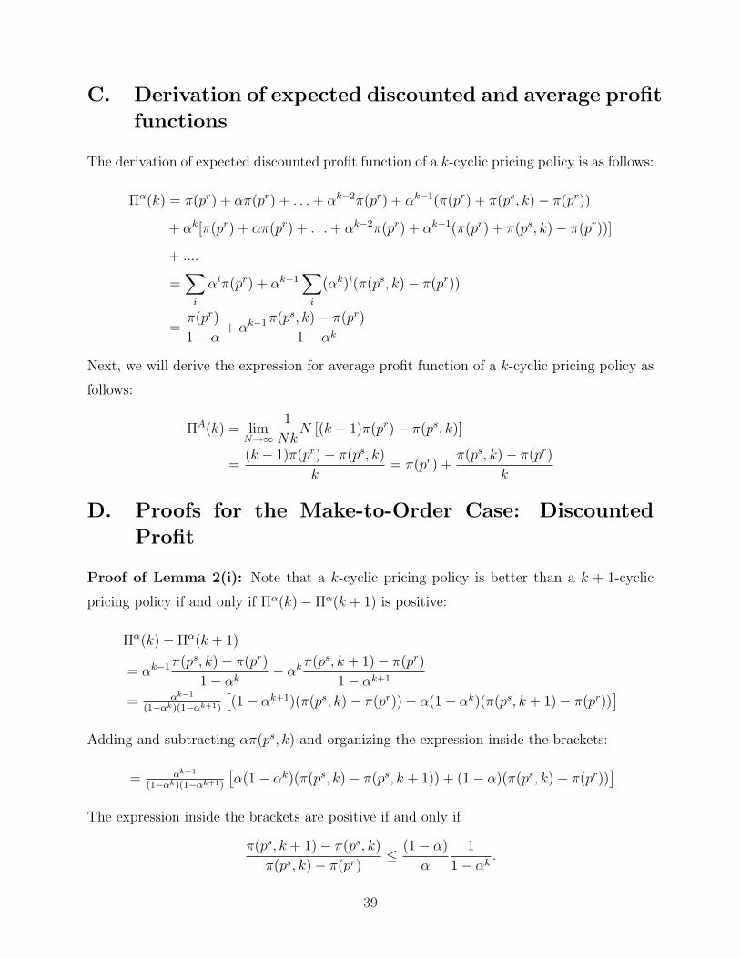
C. Derivation of expected discounted and average profit

functions

The derivation of expected discounted profit function of a k-cyclic pricing policy is as follows:

Πα(k) = π(pr) + απ(pr) + . . . + αk−2π(pr) + αk−1(π(pr) + π(ps, k)− π(pr))

+ αk[π(pr) + απ(pr) + . . . + αk−2π(pr) + αk−1(π(pr) + π(ps, k)− π(pr))]

+ ....

=∑

i

αiπ(pr) + αk−1∑

i

(αk)i(π(ps, k)− π(pr))

=π(pr)

1− α+ αk−1π(ps, k)− π(pr)

1− αk

Next, we will derive the expression for average profit function of a k-cyclic pricing policy as

follows:

ΠA(k) = limN→∞

1

NkN [(k − 1)π(pr)− π(ps, k)]

=(k − 1)π(pr)− π(ps, k)

k= π(pr) +

π(ps, k)− π(pr)

k

D. Proofs for the Make-to-Order Case: Discounted

Profit

Proof of Lemma 2(i): Note that a k-cyclic pricing policy is better than a k + 1-cyclic

pricing policy if and only if Πα(k)− Πα(k + 1) is positive:

Πα(k)− Πα(k + 1)

= αk−1π(ps, k)− π(pr)

1− αk− αk π(ps, k + 1)− π(pr)

1− αk+1

= αk−1

(1−αk)(1−αk+1)

[(1− αk+1)(π(ps, k)− π(pr))− α(1− αk)(π(ps, k + 1)− π(pr))

]

Adding and subtracting απ(ps, k) and organizing the expression inside the brackets:

= αk−1

(1−αk)(1−αk+1)

[α(1− αk)(π(ps, k)− π(ps, k + 1)) + (1− α)(π(ps, k)− π(pr))

]

The expression inside the brackets are positive if and only if

π(ps, k + 1)− π(ps, k)

π(ps, k)− π(pr)≤ (1− α)

α

1

1− αk.

39

Proof of Lemma 2(ii):

Using the previous lemma, we will show that if Πα(k) ≥ Πα(k + 1), i.e.,

π(ps, k + 1)− π(ps, k)

π(ps, k)− π(pr)≤ 1

α

(1− α)

1− αk=

1

α∑k

i=1 αi−1

then Πα(k + 1) ≥ Πα(k + 2), i.e.

π(ps, k + 2)− π(ps, k + 1)

π(ps, k + 1)− π(pr)≤ 1

α

(1− α)

1− αk+1=

1

α∑k+1

i=1 αi−1.

Note that

π(ps, k + 1)− π(ps, k)

π(ps, k)− π(pr)=

1π(ps,k)−π(pr)

π(ps,k+1)−π(ps,k)

=1

π(ps,k)−π(ps,k−1)+π(ps,k−1)−π(ps,k−2)+...+π(ps,1)−π(pr)π(ps,k+1)−π(ps,k)

=1

π(ps,k)−π(ps,k−1)π(ps,k+1)−π(ps,k)

+ π(ps,k−1)−π(ps,k−2)π(ps,k+1)−π(ps,k)

+ . . . + π(ps,1)−π(pr)π(ps,k+1)−π(ps,k)

≤ 1

α∑k

i=1 αi−1

which implies that

π(ps, k)− π(ps, k − 1)

π(ps, k + 1)− π(ps, k)+

π(ps, k − 1)− π(ps, k − 2)

π(ps, k + 1)− π(ps, k)+. . .+

π(ps, 1)− π(pr)

π(ps, k + 1)− π(ps, k)≥ α

k∑i=1

αi−1.

Multiplying each term in the left hand side with π(ps,k+1)−π(ps,k)π(ps,k+2)−π(ps,k+1)

does not change the in-

equality since π(ps,k+1)−π(ps,k)π(ps,k+2)−π(ps,k+1)

> 1;

π(ps, k)− π(ps, k − 1)

π(ps, k + 2)− π(ps, k + 1)+

π(ps, k − 1)− π(ps, k − 2)

π(ps, k + 2)− π(ps, k + 1)+. . .+

π(ps, 1)− π(pr)

π(ps, k + 2)− π(ps, k + 1)≥ α

k∑i=1

αi−1.

If we add π(ps,k+1)−π(ps,k)π(ps,k+2)−π(ps,k+1)

to the left hand side and αk+1 to the right side, the inequality

still holds since π(ps,k+1)−π(ps,k)π(ps,k+2)−π(ps,k+1)

> 1 > αk+1 due to the fact that that π(ps, k) is concave

increasing and α < 1. Hence, we obtain:

π(ps, k + 1)− π(ps, k)

π(ps, k + 2)− π(ps, k + 1)+

π(ps, k)− π(ps, k − 1)

π(ps, k + 2)− π(ps, k + 1)+. . .+

π(ps, 1)− π(pr)

π(ps, k + 2)− π(ps, k + 1)≥ α

k+1∑i=1

αi−1

which in turn implies that

π(ps, k + 2)− π(ps, k + 1)

π(ps, k + 1)− π(pr)≤ 1

α∑k+1

i=1 αi−1.

Proof of Theorem 5

40

(i) Recall that the expected discounted profit of k-cyclic pricing policy is

Πα(k) =π(pr)

1− α+ αk−1π(ps, k)− π(pr)

1− αk= Πα

r + αk−1π(ps, k)− π(pr)

1− αk

where Παr = π(pr)

1−αis the expected discounted profit of constant regular pricing policy.

Note that Παr ≥ Πα(k) if and only if π(pr) ≥ π(ps, k) for all k.

(ii) The uniqueness comes from the unimodality of Πα(k) in k. Using (4.1) and the uni-

modality of Πα(k) in k, cyclic pricing with cycle length k∗ generates more profit than

any cycle length k < k∗ and k > k∗ if and only if

π(ps, k∗)− π(ps, k∗ − 1)

π(ps, k∗ − 1)− π(pr)>

1− α

α

1

1− αk∗−1

and

π(ps, k∗ + 1)− π(ps, k∗)π(ps, k∗)− π(pr)

<1− α

α

1

1− αk∗

which implies that k∗ is the smallest integer satisfying condition (4.1).

E. Proofs for the Make-to-Order Model: Average Profit

Case

Proof of Lemma 3(i): Note that a k-cyclic pricing policy is better than a k + 1-cyclic

pricing policy if and only if ΠA(k)− ΠA(k + 1) is positive:

ΠA(k)− ΠA(k + 1) =π(ps, k)− π(pr)

k− π(ps, k + 1)− π(pr)

k + 1= 1

k(k+1)[(k + 1)(π(ps, k)− π(pr))− k(π(ps, k + 1)− π(pr))]

= 1k(k+1)

[k(π(ps, k)− π(ps, k + 1)) + (π(ps, k)− π(pr))] .

The expression inside the brackets are positive if and only if

π(ps, k + 1)− π(ps, k)

π(ps, k)− π(pr)≤ 1

k.

Proof of Lemma 3(ii): We will show that if ΠA(k) ≥ ΠA(k+1) then ΠA(k+1) ≥ ΠA(k+2).

We know that ΠA(k) ≥ ΠA(k + 1) if and only if

π(ps, k + 1)− π(ps, k)

π(ps, k)− π(pr)≤ 1

k

41

which implies that

k(π(ps, k + 1)− π(ps, k)) ≤ π(ps, k)− π(pr).

Adding and subtracting π(ps, k + 1) to the right hand side and organizing the expression:

(k + 1)(π(ps, k + 1)− π(ps, k)) ≤ π(ps, k + 1)− π(pr).

Since π(ps, k) is concave increasing in k, we obtain:

(k + 1)(π(ps, k + 2)− π(ps, k + 1)) ≤ (k + 1)(π(ps, k + 1)− π(ps, k)) ≤ π(ps, k + 1)− π(pr)

which implies thatπ(ps, k + 2)− π(ps, k + 1)

π(ps, k + 1)− π(pr)≤ 1

k + 1

hence ΠA(k + 1) ≥ ΠA(k + 2).

Proof of Theorem 5

(i) Recall that the expected average profit of a k-cyclic pricing policy is

ΠA(k) = π(pr) +π(ps, k)− π(pr)

k= ΠA

r +π(ps, k)− π(pr)

k

where ΠAr is the expected average profit of constant regular pricing policy. Note that

ΠAr ≥ ΠA(k) if and only if π(pr) ≥ π(ps, k) for all k.

(ii) The uniqueness comes from the unimodality of ΠA(k) in k. Using (4.2) and unimodality

of ΠA(k) in k, a cyclic pricing with cycle length k∗ generates more profit than any cycle

length k < k∗ and k > k∗ if and only if

π(ps, k∗)− π(ps, k∗ − 1)

π(ps, k∗ − 1)− π(pr)>

1

k∗

and

π(ps, k∗ + 1)− π(ps, k∗)π(ps, k∗)− π(pr)

<1

k∗

which implies that k∗ is the smallest integer satisfying condition (4.2).

42

F. Proof of Theorem 6

Proof. As in the lost sale case, we write Jt(y, p; k) as a convolution of two functions:

Jt(y, p; k) =

∫ ∞

0

Gt(y − ξ; p, k)φt(ξ|p, k)dξ

where Gt(w; p, k) is given as follows:

Gt(w; p, k) =π(p, k)− (1− α)c[w]+ + (1− α)c[w]− − h+[w]+ − h−[w]− + αVt+1(w, kt+1)

=π(p, k)− (h+ + (1− α)c)[w]+ − (h− − (1− α)c)[w]− + αVt+1(w, kt+1) (F.1)

where π(p, k) = (p − c)E[ξ(p, k)], thus π(p, k) = (pr − c)µr when p = pr and π(p, k) =

(ps − c)µsk when p = ps.

Since ξ(p, k) is strongly unimodal, it is sufficient to show that Gt(w; p, k) is unimodal in

w for a given p and k. We will do this by induction on t.

Suppose t = T . From our assumption, VT+1 = 0. The first term in equation (F.1),

π(p, k), is constant in x. From Assumption 4, the sum of the second and third terms is

unimodal function and is maximized when w = 0. Therefore, GT (w; p, k) is unimodal in w

and is maximized at w = 0, and JT (y, p; k) is unimodal in y.

Suppose the result holds for period t + 1 and consider Gt(w; k, p). Once again, the first

three terms of equation (F.1) are the same as in t = T , and therefore the sum of these three

terms is unimodal in w and maximized at w = 0. We complete the proof by showing that

the last term (i.e. αVt+1(w, kt+1)) is non-increasing in w and maximized at w = 0. From

the induction hypothesis that Gt+1(w; p, k) is unimodal in w, Jt+1(y, p; k) is unimodal in y.

From the fact that pr > ps > c and the fact that h− > (1 − α)c, it can be easily shown

through a sample path argument that it is suboptimal to not satisfy the existing backorder.

Thus, arg maxy Jt+1(y, p; k) ≥ 0, and maxy≥w Jt+1(y, p; k) is non-increasing in w. As a result,

maxy≥0 Jt+1(y, p; k) contains the maximum. This implies that

Vt+1(w, kt+1) = max

{maxy≥w

Jt+1(y, pr; k). maxy≥w

Jt+1(y, ps; k)

}

is also non-increasing in w and achieves the maximum at w = 0. Since the sum of unimodal

functions which have the same maximizer (mode) is also unimodal, Gt(w; k, p) is unimodal

in w.

43

G. Proof of Theorem 7

Proof. We prove this by induction. Suppose t = T .

(i) Since VT+1(x, k) = 0 for all x ≥ 0,

JT (y, pr; k) =

∫ ∞

0

[π(p, k)− (h+ + (1− α)c)[y − ξ]+ − (h− − (1− α)c)[y − ξ]−

]φ(ξ; pr, k)dξ

= π(p, k)−∫ y

0

(h+ + (1− α)c)(y − ξ)φ(ξ; pr, k)dξ −∫ ∞

y

(h− − (1− α)c)(ξ − y)φ(ξ; pr, k)dξ

The derivative of JT (y, pr; k) with respect to y, J′

T (y, pr; k) is written as follows:

J′

T (y, pr; k) =

∫ ∞

y

(h− − (1− α)c)φ(ξ; pr, k)dξ −∫ y

0

(h+ + (1− α)c)φ(ξ; pr, k)dξ

= (h− − (1− α)c)− Φr(y)(h+ + h−)

where Φr(y) is the cumulative distribution of regular demand. Since JT (y, pr; k) is

unimodal in y and arg max JT (y, pr; k) ≥ 0 by Theorem 6, we find the maximizer (i.e.

the base stock level under the regular price) by equating the J′

T (y, pr; k) to zero and

solving for y, which yields

sT (pr, k) = (Φr)−1

(h− − (1− α)c

h+ + h−

∣∣∣∣ pr, k

)

where (Φr)−1(·|pr, k) is the inverse function of cumulative distribution of regular de-

mand and h−−(1−αc)h++h− is the critical-fractile associated with a newsvendor facing regular

demand. Since Φr(y) does not depend on k, sT (pr, k) is constant in k. We will denote

regular base stock level sr.

(ii) Taking the derivative of JT (y, ps; k) with respect to y, we have

J′

T (y, ps; k) = (h− − (1− α)c)− Φsk(y)(h+ + h−)

where Φsk(·) is the cumulative distribution function of sale demand given that k periods

have passed since the last sale. Equating the J′

T (y, ps; k) to zero and solving for y yields

sT (ps, k) = (Φsk)−1

(h− − (1− α)c

h+ + h−

∣∣∣∣ pr, k

)

where (Φsk)−1(·|ps, k) is the inverse function of cumulative distribution of the sale de-

mand when k periods have passed since the last sale. Since ξr ≤ST ξsk for all k ≥ 1,

Φr(y) ≥ Φsk(y) for all y, sT (ps, k) ≥ sr.

44

(iii) The fact that JT (y, p; k) is unimodal in y and part (ii) above (that is, sr ≤ sT (ps, k)

for all k) together imply that, for x ≤ sr,

VT (x, k) = maxp∈{pr,ps}

{maxy≥x

JT (y, p; k)

}

= max[JT (sr, pr; k), JT (sT (ps, k), ps; k)]

Hence, VT (x, k) is a constant for x ≤ sr. For x ≤ sr, note that

VT (x, k) = maxp∈{pr,ps}

{maxy≥x

JT (y, p; k)

}

= max[JT (x, pr; k), JT (max[x, sT (ps, k)], ps; k)]

Since both JT (x, pr; k) and JT (max[x, sT (ps, k)], ps; k) are continuous and non-increasing

in x, VT (x, k) is also continuous and non-increasing in x.

Now, suppose the results hold for period t + 1, and consider period t:

(i) Since Jt(y, pr; k) is unimodal in y by Theorem 6, it is sufficient to show that sr satisfies

the first order condition. From the induction hypothesis, Vt+1(x; k) is constant (i.e.,

V′t+1(x; k) = 0) for x ≤ sr and non-increasing afterwards. For y ≤ sr, the derivative of

Jt(y, pr; k) with respect to y is

J′

t (y, pr; k) = (h− − (1− α)c)− Φr(y)(h+ + h−).

Solving for y, we have

sT (pr, k) = (Φr)−1

(h− − (1− α)c

h+ + h−|pr, k

)for all k.

From the induction hypothesis and the fact that Jt(y, pr; k) is unimodal in y, Jt(y, pr; k)

achieves the maximum at y = sr.

(ii) Note that, for any y ≤ sr, w = y − ξ(p, k) ≤ sr. Thus, Vt+1(w, k) remains constant for

all w ≤ sr and

J′

t (y, ps; k) = (h− − (1− α)c)− Φsk(y)(h+ + h−) for y ≤ sr.

Since ξr ≤st ξsk, J

′t (y, ps; k)

∣∣∣y=sr

≥ J′

T (y, pr; k)∣∣∣y=sr

= 0, st(ps; k) must be greater than

or equal to sr for all k.

(iii) The result follows immediately from the observation that st(ps, k) ≥ sr.

45