Embed Size (px)
Citation preview

Inventory control systems with commitment lead time
Citation for published version (APA):Ahmadi, T. (2019). Inventory control systems with commitment lead time. Technische Universiteit Eindhoven.https://doi.org/10.6100/71262ae9-f691-43f7-9d32-f97b5eea917a
DOI:10.6100/71262ae9-f691-43f7-9d32-f97b5eea917a
Document status and date:Published: 11/03/2019
Document Version:Publisher’s PDF, also known as Version of Record (includes final page, issue and volume numbers)
Please check the document version of this publication:
• A submitted manuscript is the version of the article upon submission and before peer-review. There can beimportant differences between the submitted version and the official published version of record. Peopleinterested in the research are advised to contact the author for the final version of the publication, or visit theDOI to the publisher's website.• The final author version and the galley proof are versions of the publication after peer review.• The final published version features the final layout of the paper including the volume, issue and pagenumbers.Link to publication
General rightsCopyright and moral rights for the publications made accessible in the public portal are retained by the authors and/or other copyright ownersand it is a condition of accessing publications that users recognise and abide by the legal requirements associated with these rights.
• Users may download and print one copy of any publication from the public portal for the purpose of private study or research. • You may not further distribute the material or use it for any profit-making activity or commercial gain • You may freely distribute the URL identifying the publication in the public portal.
If the publication is distributed under the terms of Article 25fa of the Dutch Copyright Act, indicated by the “Taverne” license above, pleasefollow below link for the End User Agreement:www.tue.nl/taverne
Take down policyIf you believe that this document breaches copyright please contact us at:[email protected] details and we will investigate your claim.
Download date: 09. Dec. 2020

Inventory Control Systems withCommitment Lead Time

This thesis is part of the Ph.D. thesis series of the Beta Research School forOperations Management and Logistics (onderzoeksschool–beta.nl) in which thefollowing Dutch universities cooperate: Eindhoven University of Technology,Maastricht University, University of Twente, VU Amsterdam, and WageningenUniversity and Research.
A catalogue record is available from the Eindhoven University of TechnologyLibrary.
ISBN: 978-90-386-4700-5
Inventory Control Systems withCommitment Lead Time
PROEFSCHRIFT
ter verkrijging van de graad van doctor aan deTechnische Universiteit Eindhoven, op gezag van derector magnificus, prof.dr.ir. F.P.T. Baaijens, voor een
commissie aangewezen door het College voorPromoties in het openbaar te verdedigenop maandag 11 maart 2019 om 16.00 uur
door
Taher Ahmadi
geboren te Mahabad, Iran

Dit proefschrift is goedgekeurd door de promotoren en de samenstelling van depromotiecommissie is als volgt:
voorzitter: prof.dr. T. Van Woensel1e promotor: prof.dr. A. G. de Kok2e promotor: prof.dr.ir I.J.B.F. Adancopromotor: dr. Z. Atanleden: prof.dr. J. S. Song (Duke University, USA)
prof.dr. S. Minner (Technical University of Munich, Germany)prof.dr. G.J.J.A.N van Houtumprof.dr. A.P. Zwart
Het onderzoek of ontwerp dat in dit proefschrift wordt beschreven is uitgevoerd inovereenstemming met de TU/e Gedragscode Wetenschapsbeoefening.

Acknowledgments
The completion of this thesis is a product of years of interaction and inspiration bya large number of colleagues and friends, whose comments, questions, criticism,support, and encouragement has left a mark on this work. I would like to take thisopportunity to express my sincere appreciation and warm gratitude to those whoassisted me in a myriad of ways.
First of all, special thanks to my first promotor, Prof. Ton de Kok, for giving me theopportunity to join the OPAC group and work under his supervision. I thank Tonwholeheartedly, for his patience, motivation, and immense knowledge. I have beenso fortunate to have his guidance and encouragement during my doctoral studies.I owe special thanks to my second promotor, Prof. Ivo Adan, whose creativityand kindness played a great role in forming my understanding of mathematicalproofs. Whenever I needed his support, he always welcomed me to his office andencouraged fruitful discussions. Last, but not least, to my copromotor, Dr. ZumbulAtan, who gave so much of her time and effort to my research and helped me passevery research milestone with success. Her constructive feedback and commentsplayed a significant role in shaping not only my research, but also my professionallife. I offer her my heartful thanks and appreciation.
I am grateful to Prof. Kumar Muthuraman for hosting me during my three-monthresearch visit at McCombs School of Business, the University of Texas at Austin. Itwas a very good experience for me and I was inspired by our discussions and hisfuturistic ideas.
Sincere thanks to my committee referees, whose suggestions and commentsenriched the thesis: Prof. Jeannette Song from Duke University; Prof. StefanMinner from the Technical University of Munich; Prof. Geert-Jan van Houtum fromOPAC group, and Prof. Bert Zwart from Mathematics Department at EindhovenUniversity of Technology.
Very special thanks go to OPAC family. Particularly, to Mrs. Jolanda Verkuijlen,Mrs. Claudine Hulsman, Mrs. Jose van Dijk, and Mrs. Christel Verlijsdonk for theirkind support and administrative assistance; to my officemates: Clara Stegehuis,Laura Restrepo, Joost de Kruijff, Bram Westerweel, and Douniel Lamghari-Idrissifor making the work environment both fun and productive; to other fellow Ph.D.colleagues: Sjors Jansen, Joni Driessen, Erwin van Wingerden, Loe Schlicher, DeniseTonissen, Peng Sun, Chiel van Oosterom, Simon Voorberg, Jelle Adan, Maarten

Driessen, Kay Peeters, Volkan Gumuskaya, Cansu Altintas, Yesim Koca, MirjamMeijer, Afonso Sampaio Oliveira, Vincent Karels, Nughthoh Kurdhi, Sami Ozarik,and Wendy Olsder who have profoundly influenced my way of thinking in the areaof my research and theirs.
I am also thankful to my colleagues and friends from my home country, whowere always there for me when I needed them and never let me feel homesick;Yousef Ghiami and Rama, Taimaz Soltani and Farnaz, Fardin Dashty, AlirezaHesaraki, Maryam Steadie Seifi, Shaya Pourmirza, Mina Farahani, Shahrzad FaghihRoohi, Ahmadreza Marandi and Zeinab, Babak Rezaee, Mostafa Parsa, SaeedPoormoaied and Mahsa, Haleh Mohseni and Babak, Zohre (Faranak) Khoobanand Mohammadreza, Mehdi Kamran and Samira, Ali Mehrabi, Mehran Mehr andHossein Akbaripour.
Looking back at my roots, I wish to thank all my teachers who encouraged mycuriosity and taught me well during my academic journey, especially my fifth-gradeelementary school teacher, Mr. Amir Haji. Without his support, I would not havehad any chance to be where I am today. Big thanks to Dr. Masoud Mahootchi, whopiqued my interest in this topic and guided me through my masters dissertationresearch.
Lastly, but most importantly, I am grateful to my family from whom I learned tolive, love, and learn. My utmost appreciation goes to my wonderful wife, Nooshin,whose endless love and support are beyond words.
Regrettably, but inevitably, this list will not be complete. I hope those who aremissing will forgive me and still accept my heartfelt thanks for their influence onmy work and my life during these years.
Taher AhmadiEindhoven, October 2018

Contents
1 Introduction 11.1 Motivation . . . . . . . . . . . . . . . . . . . . . . . . . . . . . . . . . . . 11.2 Inventory Systems . . . . . . . . . . . . . . . . . . . . . . . . . . . . . . 4
1.2.1 System 1: A Single-location Inventory System . . . . . . . . . . 41.2.2 System 2: A Single-location Inventory System with Commit-
ment and Service Constraint . . . . . . . . . . . . . . . . . . . . 51.2.3 System 3: A Two-component, Single-end-product ATO System 5
1.3 Overview and Contributions of the Thesis . . . . . . . . . . . . . . . . 61.4 Outline of the Thesis . . . . . . . . . . . . . . . . . . . . . . . . . . . . . 7
2 Literature Review 92.1 Single-location Inventory Systems with ADI . . . . . . . . . . . . . . . 9
2.1.1 Perfect ADI . . . . . . . . . . . . . . . . . . . . . . . . . . . . . . 92.1.2 Imperfect ADI . . . . . . . . . . . . . . . . . . . . . . . . . . . . . 11
2.2 Multi-echelon Inventory Systems with ADI . . . . . . . . . . . . . . . . 132.3 Exposition of the Research . . . . . . . . . . . . . . . . . . . . . . . . . . 15
3 A Single-location System 173.1 Introduction . . . . . . . . . . . . . . . . . . . . . . . . . . . . . . . . . . 173.2 Problem Formulation . . . . . . . . . . . . . . . . . . . . . . . . . . . . . 203.3 Analysis . . . . . . . . . . . . . . . . . . . . . . . . . . . . . . . . . . . . 22
3.3.1 Analysis of the Cost Function . . . . . . . . . . . . . . . . . . . . 233.3.2 The Structure of the Optimal Policy . . . . . . . . . . . . . . . . 24
3.4 Linear Commitment Cost . . . . . . . . . . . . . . . . . . . . . . . . . . 263.4.1 Sensitivity Analysis on the Unit Commitment Cost Threshold . 273.4.2 Numerical Analysis on C(sψ, ψ) . . . . . . . . . . . . . . . . . . 293.4.3 Optimal Commitment Lead Time for a Given Base-stock Level 313.4.4 Profitability of the Optimal Policy . . . . . . . . . . . . . . . . . 33
3.5 Conclusion . . . . . . . . . . . . . . . . . . . . . . . . . . . . . . . . . . . 343.6 Appendix A: Proofs . . . . . . . . . . . . . . . . . . . . . . . . . . . . . . 37
3.6.1 Proof of Lemma 3.1 . . . . . . . . . . . . . . . . . . . . . . . . . 373.6.2 Proof of Lemma 3.2 . . . . . . . . . . . . . . . . . . . . . . . . . 383.6.3 Proof of Theorem 3.1 . . . . . . . . . . . . . . . . . . . . . . . . . 393.6.4 Proof of Theorem 3.2 . . . . . . . . . . . . . . . . . . . . . . . . . 403.6.5 Proof of Corollary 3.1 . . . . . . . . . . . . . . . . . . . . . . . . 43

3.6.6 Proof of Corollary 3.2 . . . . . . . . . . . . . . . . . . . . . . . . 433.6.7 Proof of Lemma 3.3 . . . . . . . . . . . . . . . . . . . . . . . . . 43
3.7 Appendix B: Compound Poisson Demand . . . . . . . . . . . . . . . . 463.7.1 Numerical Results . . . . . . . . . . . . . . . . . . . . . . . . . . 50
4 A Single-location System with Service Constraint 534.1 Introduction . . . . . . . . . . . . . . . . . . . . . . . . . . . . . . . . . . 534.2 Problem Formulation . . . . . . . . . . . . . . . . . . . . . . . . . . . . . 564.3 Analysis . . . . . . . . . . . . . . . . . . . . . . . . . . . . . . . . . . . . 57
4.3.1 Probability Distribution of Waiting Time . . . . . . . . . . . . . 584.3.2 Cost Function . . . . . . . . . . . . . . . . . . . . . . . . . . . . . 614.3.3 Constraints on the Customer Waiting Time . . . . . . . . . . . . 62
4.4 Solution Methodology . . . . . . . . . . . . . . . . . . . . . . . . . . . . 694.4.1 The Exact Optimization Algorithm . . . . . . . . . . . . . . . . 694.4.2 The Heuristic Optimization Algorithm . . . . . . . . . . . . . . 694.4.3 Performance Evaluation of the Heuristic Algorithms . . . . . . 70
4.5 Comparisons . . . . . . . . . . . . . . . . . . . . . . . . . . . . . . . . . . 714.5.1 The ACO Model vs. the CCO Model . . . . . . . . . . . . . . . 714.5.2 Average Waiting Time vs. Backordering Cost . . . . . . . . . . 724.5.3 The Value of the Commitment Lead Time . . . . . . . . . . . . 73
4.6 Conclusion . . . . . . . . . . . . . . . . . . . . . . . . . . . . . . . . . . . 744.7 Appendix: Proofs . . . . . . . . . . . . . . . . . . . . . . . . . . . . . . . 76
4.7.1 Proof of Theorem 4.1 . . . . . . . . . . . . . . . . . . . . . . . . . 764.7.2 Proof of Lemma 4.1 . . . . . . . . . . . . . . . . . . . . . . . . . 774.7.3 Proof of Proposition 4.1 . . . . . . . . . . . . . . . . . . . . . . . 784.7.4 Proof of Lemma 4.2.1 . . . . . . . . . . . . . . . . . . . . . . . . 794.7.5 Proof of Lemma 4.2.2 . . . . . . . . . . . . . . . . . . . . . . . . 804.7.6 Proof of Lemma 4.3 . . . . . . . . . . . . . . . . . . . . . . . . . 804.7.7 Proof of Proposition 4.2.1 . . . . . . . . . . . . . . . . . . . . . . 804.7.8 Proof of Proposition 4.2.2 . . . . . . . . . . . . . . . . . . . . . . 814.7.9 Proof of Proposition 4.3 . . . . . . . . . . . . . . . . . . . . . . . 814.7.10 Proof of Proposition 4.4.1 . . . . . . . . . . . . . . . . . . . . . . 814.7.11 Proof of Proposition 4.4.2 . . . . . . . . . . . . . . . . . . . . . . 824.7.12 Proof of Proposition 4.4.3 . . . . . . . . . . . . . . . . . . . . . . 824.7.13 Proof of Lemma 4.4 . . . . . . . . . . . . . . . . . . . . . . . . . 824.7.14 The Heuristic Algorithm for ACO Model . . . . . . . . . . . . . 834.7.15 The Heuristic Algorithm for CCO Model . . . . . . . . . . . . . 834.7.16 The Exact Optimization Algorithm for ACO Model . . . . . . . 844.7.17 The Exact Optimization Algorithm for CCO Model . . . . . . . 85
5 An ATO System 875.1 Introduction . . . . . . . . . . . . . . . . . . . . . . . . . . . . . . . . . . 875.2 Problem Formulation . . . . . . . . . . . . . . . . . . . . . . . . . . . . . 89
5.2.1 Commitment Lead Time . . . . . . . . . . . . . . . . . . . . . . . 91
5.2.2 Net Inventory Levels . . . . . . . . . . . . . . . . . . . . . . . . . 925.2.3 Remnant Inventory Levels . . . . . . . . . . . . . . . . . . . . . . 945.2.4 Long-run Average Cost . . . . . . . . . . . . . . . . . . . . . . . 95
5.3 Characterization of the Optimal Control Policies . . . . . . . . . . . . . 975.3.1 Optimization of the Component Base-stock Levels . . . . . . . 975.3.2 Unit Commitment Cost Thresholds . . . . . . . . . . . . . . . . 1005.3.3 Optimization of the Commitment Lead Time . . . . . . . . . . . 102
5.4 Numerical Results . . . . . . . . . . . . . . . . . . . . . . . . . . . . . . 1045.5 Conclusion . . . . . . . . . . . . . . . . . . . . . . . . . . . . . . . . . . . 1055.6 Appendix: Proofs . . . . . . . . . . . . . . . . . . . . . . . . . . . . . . . 108
5.6.1 Proof of Proposition 5.1 . . . . . . . . . . . . . . . . . . . . . . . 1085.6.2 Simplification of Equation (5.2.4) . . . . . . . . . . . . . . . . . . 1095.6.3 Derivation of Equation (5.6) . . . . . . . . . . . . . . . . . . . . . 1105.6.4 Derivation of Expression (5.7) . . . . . . . . . . . . . . . . . . . . 1105.6.5 Proof of Theorem 5.1 . . . . . . . . . . . . . . . . . . . . . . . . . 1105.6.6 Proof of Theorem 5.2 . . . . . . . . . . . . . . . . . . . . . . . . . 1135.6.7 Proof of Lemma 5.1 . . . . . . . . . . . . . . . . . . . . . . . . . 1165.6.8 Proof of Theorem 5.3 . . . . . . . . . . . . . . . . . . . . . . . . . 1175.6.9 Proof of Theorem 5.4 . . . . . . . . . . . . . . . . . . . . . . . . . 117
6 Conclusions 1216.1 Results and Findings . . . . . . . . . . . . . . . . . . . . . . . . . . . . . 1226.2 Further Research . . . . . . . . . . . . . . . . . . . . . . . . . . . . . . . 125
Bibliography 127
Summary 133
About the author 135


1Introduction
1.1. Motivation
The majority of supply chain glitches occur due to lack of alignment betweendemand and supply. Supply chain uncertainties make it almost impossible tocome up with a silver bullet for this problem. Uncertainties from both supplyand demand sides result in a mismatch between supply and demand. As a well-known approach to overcome this mismatch, inventories are kept throughout thesupply chain network in different forms such as; raw materials, modules, and end-products. Although inventories can serve to hedge against possible supply anddemand uncertainties, they can erode the profitability of the system by imposingunnecessary costs. Hence, inventories may improve the responsiveness of thesystem, on the one hand, they may deteriorate the cost-effectiveness of the system,on the other. For instance, holding excess inventories imposes unnecessary inventoryholding costs to the system. These costs can be referred to as the opportunity costof capital tied up in inventory, costs of storage and material handling, labor, andinsurance costs. Particularly, in high-tech companies with technological products,in addition to the above-mentioned inventory costs, inventory obsolescence costmay be charged.
Moreover, lack of inventories can also causes products shortage and, in turn, canresult in late deliveries to the customers and customer dissatisfaction. In this case,the firm has to pay a shortage penalty cost that can be referred to all the costsassociated with tardiness. Although calculating the shortage penalty costs is not astraightforward task, it can be interpreted as penalties for the lateness in delivery,loss of customers’ goodwill, profit, and even the business. In a shortage situation,customers may tolerate and wait for the availability of the product or may not
2 Chapter 1. Introduction
tolerate and find another source to get the product. Since in the former case demandis backoredered and in the latter, it is lost, the associated shortage cost with eachcase is called backordring cost and lost sale cost, respectively.
To date, scholars have contributed to the literature of inventory management byproposing various approaches to find the trade-off between the holding inventoryand shortage penalty costs that are correlated negatively. Hence, keeping moreinventory increases the holding cost while decreases the shortage penalty cost andvice versa. A trade-off between these two types of costs can guarantee an optimalsystem performance in terms of cost-effectiveness and responsiveness.
One of the barriers that makes this trade-off more and more challenging iscustomer demand information uncertainty. There is an increasing consensusamong researchers and practitioners that obtaining and sharing customer demandinformation with all the partners of a supply chain enhances the coordination andeventually the performance of the system. The role of sharing customer demandinformation for supply chain performance is more magnified if this informationis shared ahead of time. This information is often referred to in the literature asAdvance Demand Information (ADI). ADI represents the customers’ information ontheir future demand at the present time.
Consider a firm that sells a product to the customers. Sharing ADI with the firmcreates a win-win cooperation for both parties i.e., the firm and customers, underwhich the supplier can use ADI to reduce its excess and stockout inventory risksand the customers reduce the risk of the product unavailability. With the help ofadvances in information technology such as Electronic Data Interchange (EDI), web-based platforms and Internet-based communication tools business firms of all thesizes can obtain ADI from their customers by implementing a preorder strategy, inwhich the customers place their order ahead of time to share the information ontiming and sizes of their future order with the firm.
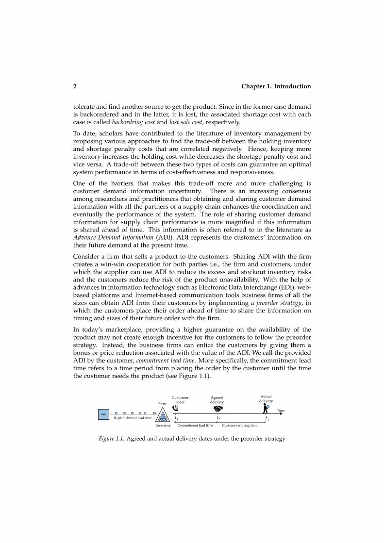
In today’s marketplace, providing a higher guarantee on the availability of theproduct may not create enough incentive for the customers to follow the preorderstrategy. Instead, the business firms can entice the customers by giving them abonus or price reduction associated with the value of the ADI. We call the providedADI by the customer, commitment lead time. More specifically, the commitment leadtime refers to a time period from placing the order by the customer until the timethe customer needs the product (see Figure 1.1).
tt t
Agreed delivery
Actual delivery
Commitment lead time Customer waiting time
Time
Customer orderFirm
1 2 3Replenishment lead time
∞
Inventory
Figure 1.1: Agreed and actual delivery dates under the preorder strategy

1.1 Motivation 3
Since longer commitment lead time can be more beneficial to the firm, the firm paysthe bonus based on the length of the commitment lead time. Even though from thecustomer’s perspective, the bonus is a kind of income, from the firm’s perspectiveit is a kind of cost. We refer to the bonus from the firm’s perspective as commitmentcost. Although the commitment lead time plays an undeniable role in improvingprofit of the firm by diminishing mismatches between demand and supply, it is nottrivial how adding commitment cost to the total cost of a conventional inventorysystem including inventory holding and backordering costs should lead to a costreduction.
It might be an intuitive concept that the commitment lead time helps the businessfirm to reduce the need for inventory or excess capacity, on the one hand, andincrease the availability of its products, on the other. As a result, the firm canreduce the inventory holding and backordering costs. But, adding commitmentcost to the system total cost need to be addressed in an analytical framework.
From the literature of the stochastic inventory management, we know that in atraditional stochastic inventory problem including holding and backordering costs,the long-run average total cost is minimized when the inventory level is adjustedsuch that both cost terms have the same magnitude. However, by adding thecommitment cost to the problem, this approach may not work. Figure 1.2 givesa schematic representation of these three costs when the objective of the firm isminimizing the long-run average total cost. In this situation, the firm’s controlpolicy is a combination of the inventory level and the length of the commitmentlead time. More specifically, the impact of each element of the control policy oneach cost term (i.e., holding, backordering, and commitment) can be viewed as athree-pan weighing scale with two balancing screws.
Inventory Level
Replenishment Lead Time of the Firm
Commitment Lead Time
h p c
Long-run Average
Total Cost
0 ∞
Min
Holding Backordering CommitmentCost Cost Cost
Figure 1.2: Representation of the inventory management with three cost terms
Each pan represents one of the cost terms and each balancing screw represents oneelement of the control policy. We aim to adjust the balancing screws such thatthe pointer of the weighing scale shows the minimum total cost. As it is seen,the inventory level effects the magnitude of the holding and backordering costs

4 Chapter 1. Introduction
and the length of commitment lead time effects the magnitude of all the three costterms. In other words, more inventory level results in more holding cost and lessbackordering cost and vice versa. Also, more commitment lead time results in morecommitment cost as well as less holding and backordering costs and vice versa. Asit is presented in Figure 1.2, when the magnitude of the holding and backorderingcosts equals the magnitude of the commitment cost, the pointer of the weighingscale does not show the minimum. Hence, the existing approach in the literaturecannot be applied to our problem.
In this thesis, we aim to investigate the pereorder strategy associated withcommitment cost from cost and service perspectives in different inventory systems.First, we analyze a single-location inventory system. Then, we extend our analysisby replacing the backordering cost with two time-based service measures. Finally,an assemble-to-order (ATO) system with two components and a single end-productis examined.
The remainder of this chapter is organized as follows: First, we provide an extensiveliterature review on ADI in single-location and multi-location inventory systems.In Section 1.2, we distinguish three inventory systems. Finally, we present theoverview and outlines of the thesis in Sections 1.3 and 1.4, respectively.
1.2. Inventory Systems
In this section, we establish the settings under which the profitability of thepreorder strategy is investigated. We mainly consider inventory systems with asingle end-product, Poisson demand, continuous review, base-stock policy, fixedreplenishment lead times, and backordered demand. By adding specific settings,we distinguish three inventory systems. In what follows, we provide a shortintroduction of inventory systems, each of which will be elaborated in a dedicatedchapter of this thesis.
1.2.1 System 1: A Single-location Inventory System
In this system, we consider a single-location inventory system that operates underpreorder strategy. We aim to find the optimal control policy as a combination of thebase-stock level and commitment lead time such that a long-run average total cost isminimized. The total cost consists of holding, backordering and commitment costs.We formulate the problem as an unconstraint mixed-integer nonlinear program toanswer the following research questions;
1. When and how should the firm use the preorder strategy?2. What are the characteristics of the optimal control policy?

1.2 Inventory Systems 5
3. Which factors have the largest impact on the benefits of the preorder strategy?
We present the related analysis and results in Chapter 3. The chapter is a slightlymodified version of Ahmadi et al. (2019b).
1.2.2 System 2: A Single-location Inventory System with Commit-ment and Service Constraint
In this system, in addition to the settings of System 1, we take time-based servicemeasures into account. We aim to find the optimal control policy such thatthe long-run average total cost consisting of holding and commitment costs isminimized subject to a time-based service constraint. We study two time-basedservice measures; average customer waiting time and individual customer waiting time.For the first measure, we put a maximum waiting threshold on the average customerwaiting time. For the second, we form a chance constraint consisting of a servicelevel as well as the maximum waiting threshold. We formulate the problem asa constraint mixed-integer nonlinear program to answer the following researchquestions;
1. When should the firm use the preorder strategy?2. How can the optimal control policy be obtained?3. What is the impact of the commitment lead time on the customer waiting time and the
optimal cost value?4. What is the impact of commitment lead time on the equivalent unit backordering cost
to maximum waiting threshold?
We present the related analysis and results in Chapter 4.
1.2.3 System 3: A Two-component, Single-end-product ATO Sys-tem
In this system, we consider a two-component, single-end product ATO system thatoperates under a preorder strategy. We aim to find the optimal control policy as acombination of component base-stock levels and the optimal commitment lead time,that minimizes the long-run average total cost consisting of components’ inventoryholding, backordering and commitment costs. We formulate the problem as anunconstraint mixed-integer nonlinear program to answer the following researchquestions;
1. When and how should the firm use the preorder strategy?

6 Chapter 1. Introduction
2. What are the characteristics of the optimal control policy?
We present the related analysis and results in Chapter 5. The chapter is a slightlymodified version of Ahmadi et al. (2019a).
1.3. Overview and Contributions of the Thesis
In this section, we provide an overview of this thesis and describe our maincontributions. The content of this thesis is presented in six chapters. Chapter 2represents the exposition of our research within the context of existing literatureon ADI in inventory systems. In Chapter 3, we study a single-location inventorysystem with preorder strategy. We prove the optimality of bang-bang and all-or-nothing policies for the commitment lead time and the base-stock policy,respectively. We study the case where the commitment cost is linear in the length ofthe commitment lead time in detail. We show that there exists a unit commitmentcost threshold which dictates the optimality of either a buy-to-order or a buy-to-stock strategy. The unit commitment cost threshold is increasing in the unitholding and backordering costs and decreasing in the mean lead time demand. Fora given base-stock level, we develop a simple and accurate approximation for thecorresponding optimal commitment lead time. Finally, we determine the conditionson the unit commitment cost for profitability of the buy-to-order strategy.
In Chapter 4, we study a single-location inventory system with preorder strategyand two time-based service constraints. We propose exact and heuristic opti-mization algorithms for each constraint optimization model. Different from theprevious chapter, we observe that when commitment lead time and time-basedservice measures are taken into account, the optimal commitment lead time isnot a bang-bang policy, anymore. We derive the exact distribution probabilityof customer waiting time in terms of system parameters and control policy. Weshow that the commitment lead time not only increases the service level (i.e., thelikelihood of meeting a customer demand up to a threshold) but also decreases thepossible maximum waiting time. Also, the optimal cost value is bounded and non-increasing in the maximum waiting threshold. We find that when the firm wants toprovide a quicker response to a higher percentage of the customers, the value of thecommitment lead time in terms of cost reduction is more highlighted. Moreover,we consider an unconstraint optimization model with backordering cost and itsequivalent constraint optimization model with the average waiting time constraint.We calculate equivalent unit backordering cost such that both models have the sameoptimal cost. We find a negative relationship between unit backordering cost andmaximum waiting threshold. When commitment lead time is taken into account,the equivalent unit backordering cost is always bounded above.
In Chapter 5, we study a two-component, single-end product ATO system with
1.4 Outline of the Thesis 7
preorder strategy. We find that the optimal commitment lead time is either zero orequals the replenishment lead time of one of the components. When the optimalcommitment lead time is zero, the preorder strategy is not beneficial and theoptimal control strategy for both components is buy-to-stock. When the optimalcommitment lead time equals the lead time of the component with the shorterlead time, the optimal control strategy for this component is buy-to-order and itis buy-to-stock for the other component. On the other hand, when the optimalcommitment lead time equals the lead time of the component with the longer leadtime, the optimal control strategy is the buy-to-order strategy for both components.We find the unit commitment cost thresholds which determine the conditions underwhich one of these three cases holds.
In Chapter 6, we conclude the thesis and represent directions as extensions forfuture work. We suggest that the preorder strategy can be studied in more complexATO systems with multiple end-products. Also, the commitment lead time conceptcan be investigated in decentralized ATO systems with the help of game theory.
1.4. Outline of the Thesis
In this thesis, the profitability of the preorder strategy in three different inventorysystem settings is investigated. For this purpose, in Chapter 2, a comprehensiveliterature review on inventory systems with ADI is provided. In Chapter 3, weconsider a single-location inventory system. We extend our analysis in Chapter4 by replacing the backordering cost with two time-based service measures. InChapter 5, the systems is extended to a two-component, single-end-product ATOsystem. Eventually, the thesis is concluded in Chapter 6 and possible extensionsare provided. Table 1.1 gives an overview of the title and system structure of eachchapter.

8 Chapter 1. Introduction
Tabl
e1.
1:Th
esis
stru
ctur
e
Cha
p.Pr
oble
mSt
ruct
ure
Titl
e1
Intr
oduc
tion
Intr
oduc
tion
2R
evie
win
gth
ere
cent
liter
atur
eon
inve
ntor
ym
anag
emen
tw
ith
AD
ILi
tera
ture
revi
ew
3t
t-ψ
t+
W
~P
ois
s (λ
)
Ag
ree
d
de
liv
ery
Act
ual
d
eli
ver
y
Com
mit
men
t co
stB
acko
rder
ing
cos
t
Tim
e
Ho
ldin
g c
ost
l∞
Cu
sto
mer
ord
er
Sing
le-l
ocat
ion
syst
emw
ith
com
mit
men
t
4t
t-ψ
t+
W
~ P
ois
s (λ
)
Ag
ree
d
de
liv
ery
Act
ual
d
eli
ver
y
ω
Com
mit
men
t co
stC
ust
omer
wai
tin
g t
ime
Tim
e
Ho
ldin
g c
ost
l∞
Cu
sto
mer
ord
er
Max
imu
m w
ait
ing
th
resh
old
t+ω
Sing
le-l
ocat
ion
syst
emw
ith
com
mit
men
tan
dti
me-
base
dse
rvic
eco
nstr
aint
5t
t-ψ
t+
W
~P
ois
s (λ
)A
gre
ed
d
eli
ver
yA
ctu
al
de
liv
ery
Com
mit
men
t co
stB
acko
rder
ing
cos
t
tim
e
∞
l∞
2
1l
Cu
sto
mer
ord
er
Ass
emb
ler
Ho
ldin
g c
ost
of
com
po
nen
t 1
Ho
ldin
g c
ost
of
com
po
nen
t 2
ATO
syst
emw
ith
com
mit
men
t
6C
oncl
udin
gre
mar
ksan
ddi
rect
ions
for
futu
rere
sear
chC
oncl
usio
ns

2Literature Review
In this chapter, we review the relevant studies to specify the exposition of ourresearch in the body of literature. Our work is related to inventory control systemswith ADI. We organize the literature review based on the system structures in twosections. First, in Section 2.1 we review single-location inventory systems with ADI.Then, we cover multi-location inventory systems with ADI in Section 2.2. Finally,Section 2.3 represents the exposition of our research.
2.1. Single-location Inventory Systems with ADI
There is a growing body of research that addresses the value of information inmanaging supply chains. The literature on inventory control systems dealingwith ADI can be broadly categorized into two classes based on the accuracy ofinformation about future orders: perfect and imperfect ADI. In the first class, thecustomers provide the firm with the exact information about the timing and thesize of their future orders. However, in the second class, customers provide thefirm with an estimate of timing or quantity of future orders which may then laterbe modified or canceled. We review studies dealing with perfect and imperfect ADIin Subsections 2.1.1 and 2.1.2, respectively.
2.1.1 Perfect ADI
One of the earliest and most influential works on perfect ADI is the work ofHariharan and Zipkin (1995). They study a single-location inventory system thatuses a continuous-review order-base-stock replenishment policy to fulfill customer

10 Chapter 2. Literature Review
orders that arrive according to a Poisson process. Each customer orders a singleitem where should be delivered after a fixed amount of time called demand leadtime. They construct an equivalent conventional model, i.e. one with no demandlead times, in which the demand lead times are subtracted from replenishmentlead times. This implies that the impact of demand lead time on overall systemperformance is the same as a system with corresponding replenishment lead timereduction. Assuming similar demand lead times for all the customers, the authorsprove the optimality of a base-stock policy.
Gilbert and Ballou (1999) study a steel distributor that manages its capacity andinventory by determining a portion of its demand as ADI. They model the problemconsidering ordering, holding and lost-sale costs. The model provides a useful toolfor estimating the cost savings associated with various levels of ADI. Chen (2001)considers a firm sells a single product in two periods. The firm offers a menuof price-delay combinations, from which the customers can choose to provide thefirm with ADI or not. He shows how the firm can determine an optimal price-delay schedule. Cattani and Souza (2002) investigate inventory-rationing policiesin a firm with a single product and two demand classes, where one class requestsfaster delivery and pays a higher price. They study several rationing policies andcompare the performance of these rationing policies under various scenarios forcustomer response to delay: lost sales, backlog, and a combination of lost sales andbacklog. Karaesmen et al. (2004) assess the value of using ADI under a variety ofassumptions and the delivery timing requirements. They, model a make-to-stockqueue. McCardle et al. (2004) study a situation, in which two retailers considerlaunching an Advance Booking Discount (ABD) program. They analyze fourpossible scenarios wherein each of the two retailers offer an ABD program or not,and establish conditions under which the unique equilibrium calls for launchingthe ABD program at both retailers.
Kocaga and Sen (2007) consider a spare-part inventory system that faces two classesof demand arrivals such that class 1 demands are due immediately, whereas class2 demands provide ADI. They conduct a case study with 64 representative partsand show that significant savings are possible through incorporation of demandlead times and rationing. Wijngaard and Karaesmen (2007) investigate orderaggregation in a capacitated production system with perfect ADI. They prove thatwhen customer order lead times are less than a threshold value, it is allowed toaggregate the orders over time. Liberopoulos (2008) finds the trade-off betweenfinished goods inventory and ADI in an inventory system. He shows that the trade-off is linear if the supply process can be modeled as an M/D/1 queue, and it is notlinear if the supply process can be modeled as an M/D/∞. Papier and Thonemann(2010) consider a rental system with two customer classes; premium and classicservice. Just under the premium service, customers provide ADI. They propose anADI policy and analyze its performance by deriving upper and lower bounds onthe optimal expected profit. Using numerical experiments, they indicate that thepotential benefit of using ADI is significant and that our ADI policy performs close

2.1 Single-location Inventory Systems with ADI 11
to optimal. Benbitour and Sahin (2015) use simulation to evaluate both type of ADI.They observe that the imperfectness of demand information reduces the benefitsof ADI. More specifically, for imperfect ADI they realize that the imperfect duedates deteriorate the systems performance more than imperfect demand quantities.Bernstein and DeCroix (2014) analyze the impact of ADI on firm profit and onthe benefits of resource flexibility with multiple products. They consider twodifferent forms of imperfect ADI as demand volume across products and demandmix between products. They find that commonality and volume information arestrategic complements, however, commonality and mix information are strategicsubstitutes.
2.1.2 Imperfect ADI
Buzacott and Shanthikumar (1994) study the impact of the forecast accuracy on thelead time and the safety stock in a material requirements planning (MRP) system.They find that the safety time is usually only preferable to safety stock when it ispossible to make accurate forecasts of future required shipments; otherwise, safetystock is more robust in confronting changes in customer requirements. Gallego andOzer (2001) prove that for an inventory system state-dependent, base-stock policiesare optimal for with and without fixed costs. Also, they determine conditions underwhich ADI has no operational value. The impact of imperfect ADI in a project-based supply chain with two types of demand is studied by van Donselaar et al.(2001). They find that imperfect ADI is particularly beneficial if it is applied inproject environments in which proposals have a high chance of turning into orders.Iyer et al. (2003) asses a capacity planning problem with demand postponementstrategy in which a fraction of the demands from the regular period are postponedand satisfied during a postponement period. They formulate the problem as a two-stage capacity planning problem and analytically determine the optimal regularand postponement period capacities.
Production planning with ADI and outsourcing is considered by Hu et al. (2003).They find that the optimal policy is a state-dependent, double-threshold policy.Ozer and Wei (2004) address a capacitated production system with the ability toobtain ADI. They establish optimal policies and characterize their behavior withrespect to capacity, fixed costs, ADI, and the planning horizon. They illustratehow ADI can be a substitute for capacity and inventory. Zhu and Thonemann(2004) consider an inventory system with ADI. They show that information costand demand correlation are important factors for determining the optimal extentof ADI sharing. Tan et al. (2007) investigate an inventory system operatingunder up-to-level policy with imperfect ADI. They show that the optimal orderingpolicy is of state-dependent order-up-to type, where the optimal order level isan increasing function of the ADI size. Liberopoulos and Koukoumialos (2008)evaluate the impact of variability and uncertainty in ADI on the performance ofa capacitated/uncapacitated system with two customer classes; one class without

12 Chapter 2. Literature Review
ADI and the other with imperfect ADI. They model the system as four differentqueuing systems.
Production control and inventory allocation in an integrated production-inventorysystem with multiple customer classes and imperfect ADI is studied by Gayonet al. (2009). They show that the optimal production and allocation policies arestate-dependent base-stock and multilevel rationing policies, respectively. Tan et al.(2009) investigate the impact of ADI on ordering and rationing decisions in aninventory system with two demand classes. They find that imperfect ADI andrationing are two important characteristics that will improve system performanceunder specific conditions. Huang and van Mieghem (2014) conduct a study on thevalue of click tracking as a mechanism to obtain imperfect ADI. Using an empiricalstudy, they show that clickstream data provides the firm with ADI in terms of notonly purchasing probabilities and amount but also purchasing timing.
Benjaafar et al. (2011) model a capacitated system with imperfect ADI as acontinuous-time Markov decision process and prove the existence of an optimalstate-dependent base-stock policy. They find that while ADI is always beneficialto the firm, this may not be the case for the customers who provide the ADI.Iravani et al. (2007) consider a capacitated supplier with two classes of customers:primary and secondary. The primary customer places a random order quantitybased on a predetermined time window; however, the secondary customer requestsa single item at a random time. If the supplier is not able to fulfill the primarycustomer order a penalty should be paid to the customer and serving the secondarycustomer results in an additional profit. They characterize the supplier’s optimalproduction and stock reservation policies. They show that these policies arethreshold-type policies and thresholds are monotone with respect to the primarycustomer’s order size. Altendorfer and Minner (2014) model a single-stage hybridproduction system in the form of either an MTO system with safety stocks or anMTS production system with ADI. Under multi-product and variable customer duedates setting, they find optimal conditions for safety stocks and safety lead timesthat minimize holding and backordering costs. Benbitour and Sahin (2015) studyboth perfect and imperfect ADI via simulation. They observe that the imperfectnessof demand information reduces the benefits of ADI. Specifically for imperfect ADI,they realize that the imperfect due dates deteriorate the system performance morethan imperfect demand quantities. Bernstein and DeCroix (2014) explore the impactof ADI on firm profit and on the benefits of resource flexibility with multipleproducts. They consider two different forms of imperfect ADI as demand volumeacross products and demand mix between products. They find that commonalityand volume information are strategic complements, however, commonality andmix information are strategic substitutes. Papier (2016) evaluates supply allocationunder sequential ADI in a capacitated system that serves different markets. Hefinds that ADI has the greatest value if the available supply is close to the initialforecasts. Topan et al. (2018) use imperfect ADI in a single-item, single-location,periodic-review inventory system with lost sale. Assuming that excess stock due

2.2 Multi-echelon Inventory Systems with ADI 13
to the imperfection of ADI can be returned to the upstream, they provide a partialcharacterization of the optimal ordering and return policy. They show that thebenefit of sharing information increases considerably if the excess stock can bereturned.
Our work in Chapters 3 and 4 belongs to Subsection 2.1.1. We study single-locationinventory systems with the preorder strategy under which the customers provideperfect ADI. Different from the literature, we assign a cost to ADI and refer to it ascommitment cost. In Chapter 3, we find the optimal replenishment and preorderstrategies such that the long-run total cost consists of holding, backordering, andcommitment costs is minimized. In Chapter 4, we replace the backordering costwith a time-based service constraint. Although the systems in both chapters aresingle location inventory system with perfect ADI, they don’t have the same optimalcontrol policies even for almost the same parameters setting.
2.2. Multi-echelon Inventory Systems with ADI
Hariharan and Zipkin (1995) study a serial system with ADI. They show thatdemand lead time can be directly subtracted from supply lead time, so that havinga demand lead time of l is equivalent to shorten supply lead time by the sameamount. Bourland et al. (1996) investigate the value of timely demand informationprovided by Electronic Data Interchange (EDI) technology in a two-stage serialsystem. They find that more accurate demand information could reduce inventoriesat the upstream stage, or improve the reliability of its deliveries to the downstreamstage, or both. The downstream stage, in turn, could reduce its inventories if itssupplier are more reliable. Lee et al. (2000) study the benefit of information sharingin a two-stage supply chain consisting of a manufacturer and a retailer. They showthat their analysis suggests that the value of demand information sharing can bequite high, especially when demands are significantly correlated over time.
Gallego and Ozer (2003) consider a serial system with ADI under periodic review.They prove the optimality of state-dependent, echelon base-stock policies for finiteand infinite horizon problems. Lu et al. (2003) study the impacts of ADI onperformance measures of a multi-component, multi-end-product ATO system withbatch Poisson arrivals. They find that ADI is more effective in improving orderfill rates than an equivalent reduction in component lead times. Ozer (2003)considers a centralized one-warehouse, multi-retailer distribution system withADI. He illustrates how ADI can be a substitute for lead times and inventory,and how it enhances the outcome of delayed differentiation. Liberopoulos andKoukoumialos (2005) investigate via simulation the trade-off between optimal base-stock and hybrid base-stock/Kanban policies in single- and two-stage capacitatedproduction/inventory systems with ADI. They indicate that when ADI is available,the echelon planned supply lead times and the number of Kanbans should be as
14 Chapter 2. Literature Review
small as possible.
Claudio and Krishnamurthy (2009) investigate the benefits of integrating ADI withKanban-based pull Production and Inventory Control Systems (PICS) in a multi-stage production system. Using simulation experiments they show that integratingADI with Kanban-based pull systems provides more opportunities for performanceimprovements compared to a pull system alone. Iida and Zipkin (2010) studythe benefits from sharing demand forecast in a supply chain with a supplierand a retailer in both cooperative and competitive settings. They form a simpletransfer-payment scheme to align the players’ incentives with that of the overallsystem. They find that unless the players’ incentives are aligned with the scheme,sharing information makes little sense. Ha et al. (2011) assess vertical informationsharing in competing supply chains with production diseconomies. They considera model of two supply chains each consisting of one manufacturer and one retailer.The retailers are engaging in Cournot or Bertrand competition. They show thatinformation sharing in one supply chain triggers a competitive reaction from theother supply chain and this reaction is damaging to the first supply chain underCournot competition but may be beneficial under Bertrand competition.
Altendorfer and Minner (2011) study the simultaneous optimization of plannedlead time and capacity invested for a two-stage MTO manufacturing system withrandom demands and random due dates. They show that when capacity ispredefined, the optimal planned lead times are independent of the distributionof customer required lead time; however, they influences the optimal capacity toinvest into. Angelus and Ozer (2016) model a multi-component, single end-productassembly system with expediting of stock and ADI. Formally, they consider anonstationary, periodic review, finite horizon, assemble-to-stock model with ADIand the option to expedite inventories of the components. They derive the structureof the optimal policy and prove that ADI and expediting of stock both reduce theamount of inventory optimally held in the system.
Nakade and Yokozawa (2016) present the theoretical analysis of a two-stageproduction inventory system with ADI, where the processing time is assumeddeterministic and identical. They derive the optimal release lead time and optimalbase-stock levels. Chintapalli et al. (2017) study a two-stage supply chain consistsof a supplier and a manufacturer. They examine whether the supplier shouldoffer advance-order discounts to encourage the manufacturer to place a portionof its order in advance, even though the manufacturer incurs some inventoryrisk. They discover that if the supplier imposes a prespecified minimum orderquantity requirement as a qualifier for the manufacturer to receive the advance-order discount, then such a combined contract can coordinate the supply chain.
Our work in Chapter 5 belongs to Section 2.2. We study a two-echelon ATOsystem consisting of two components and a single end-product. Different from theliterature, we assign a cost to ADI and find the optimal replenishment and preorderstrategies such that the long-run total cost is minimized.

2.3 Exposition of the Research 15
2.3. Exposition of the Research
Although extensive research has been done on production/inventory managementwith ADI in the last decades, we believe that allocating cost to ADI, i.e., commitmentcost, and studying its impact on the optimal control policies and the systemperformance has not been addressed, yet. In this thesis, we consider inventorysystems with a single end-product, Poisson demand, continuous review, base-stockpolicy, fixed replenishment lead times, and backordered demand. The closeststudy to our research is by Hariharan and Zipkin (1995). The authors studysingle- and multi-location inventory systems with continuous-review, single item,Poisson demand, and perfect ADI. The authors prove the optimality of a base-stock policy for the single-location inventory system. Different from Hariharanand Zipkin (1995), we have an additional cost term, which is the commitment cost.In addition to the base-stock level, we also optimize the commitment lead time.Therefore, we investigate the impact of commitment cost on the optimal controlpolicies as a combination of base-stock level(s) and commitment lead time in (1) asingle-location inventory system, (2) a single-location inventory system with a time-based service level constraint, and (3) a two-component, single-end-product ATOsystem. We contribute to the body of inventory and service management literatureby answering the corresponding research questions to each inventory system andproviding managerial insights.


3A Single-location Inventory System
with Commitment
3.1. Introduction
The consequences of demand and supply uncertainties and eventual mismatchbetween demand and supply are well-known to many companies. The need fordesigning company operations such that this mismatch is minimized or avoided hasmotivated many researchers and resulted in a rich literature on demand and supplymanagement. Among the various methods, information sharing has received a lotof attention. The benefits of acquiring and providing information about futuredemand are undeniable. Having information on future customer demand helpscompanies in reducing their inventory levels without sacrificing high service levels.Customers, who provide information on the timing and quantity of their futuredemand get a high quality service.
One way to obtain advance demand information (ADI) is implementing a preorderstrategy, in which customers place orders ahead of their actual need. The preorderstrategy is characterized by a commitment lead time which is defined as the timethat elapses between the moment an order is communicated by the customer andthe moment the order must be delivered to the customer. Although in today’scompetitive market firms cannot force their customers to place orders before theiractual need, they can tempt them to follow the preorder strategy by giving a bonus.In order to make long commitment lead times acceptable and attractive, companiesshould propose bonuses which increase with the length of commitment lead times.The commitment lead time contracts reduce the companies’ demand uncertaintyrisk and the customers’ inventory unavailability risk (Lutze and Ozer, 2008). The
18 Chapter 3. A Single-location System
form of ADI which is considered in this study is different from that of existingliterature. In the existing literature, ADI helps to make a better forecast of thefuture customer demand. In our work, the demand distribution is known. ADI isutilized operationally to reduce demand-supply mismatching by reducing the leadtime demand uncertainty. Under the optimal solution, lower lead time demanduncertainty results in lower holding and backordering costs. This form of ADIworks for service and custom-production companies, where service customers canmake reservations and customers of custom products order in advance of theirneeds (Hariharan and Zipkin, 1995).
In the Business-To-Business (B2B) environment this is typically the case when thecustomer is planning production to efficiently exploit resources, whereby plans arefrozen a few weeks ahead of time. Thus the moment of need for materials withshort shipment lead times is known earlier and the supplier can be informed aboutit. By doing so, the supplier can save on inventory holding cost and exploit the earlydemand information to produce more efficiently. The latter impact is out of scopeof this study. Also in the Business-To-Consumer (B2C) environment many onlinepurchases are not time-critical, such as books and electronic devices, and a bonusmay seduce the customer to accept a later moment of delivery. Once identifyingthe possible mutual benefit of early order placement, the question arises whatcommitment lead time should be chosen. Thus, incentifying customers to informtheir supplier earlier than the point in time determined by the moment of need andthe shipment lead time may substantially reduce cost for the supplier, while hardlyhaving an impact on the customer cost. This study discusses both the potentialbenefits of preordering and the optimal commitment lead time choice.
We study the preorder strategy of a firm in a single item, single location setting.The firm faces random customer demand and uses a continuous-review base-stock policy to replenish its inventory from an uncapacitated supplier with adeterministic lead time. Under the aforementioned setting, the firm offers apreorder strategy to its customers and consequently, they receive a bonus. From thefirm’s perspective, the bonus is kind of cost. We refer to this cost as a commitmentcost. The commitment cost function is strictly increasing and convex in the lengthof the commitment lead time. Since a commitment lead time longer than thereplenishment lead time does not have any effect on reducing the lead time demanduncertainty, the commitment lead time is bounded by zero and the length of thereplenishment lead time. The firm aims to evaluate this preorder strategy and findthe optimal length of the commitment lead time and the optimal base-stock level,which minimize the total long-run average cost. This cost is the sum of long-runaverage holding, backordering and commitment costs. We formulate the total long-run average cost and answer the following questions:
1. When and how should the firm use the preorder strategy?Based on the structure of the commitment cost, we find the sufficientconditions under which the firm should offer the preorder strategy. More

3.1 Introduction 19
specifically, assuming a linear commitment cost per time unit, we find a unitcommitment cost threshold such that for any unit commitment cost below thethreshold it is better for the firm to offer the preorder strategy. The thresholdis a function of the mean lead time demand, holding and backordering unitcosts. By means of this unit commitment cost threshold the firm can decidewhether offering the preorder strategy is cost effective or not. When thepreorder strategy is beneficial to the firm, the firm should choose a strategythat is similar in spirit to a make-to-order production strategy. In our context,we call this a buy-to-order (BTO) strategy. When preordering is not beneficial,the firm should a strategy that is similar in spirit to a pure make-to-stockproduction strategy. In our context, we call this a buy-to-stock (BTS) strategy.
2. What are the characteristics of the optimal control policy?The optimal commitment lead time and the optimal base-stock level are notindependent from each other. We characterize the optimal base-stock level andits corresponding optimal commitment lead time. We prove the optimality ofbang-bang and all-or-nothing policies for the commitment lead time and thebase-stock policy, respectively. We show that the optimal commitment leadtime is either zero or equal to the replenishment lead time. We show thatwhen the commitment lead time is zero, the corresponding base-stock levelis the solution of the well-known Newsvendor problem with deterministiclead time and when the commitment lead time equals the replenishment leadtime, the corresponding optimal base-stock level is zero. Consistent with theliterature we call this policy as an all-or-nothing policy (Lutze and Ozer, 2008).
3. Which factors have the largest impact on the benefits of the preorder strategy?Through exact sensitivity analysis on the unit commitment cost threshold, weprovide insights on the benefits of the preorder strategy. We find that thepreorder strategy helps with high demand uncertainty, even when the unitcommitment cost is high. Similarly, the preorder strategy benefits the firmwhen the unit holding and backordering costs increase, even when the unitcommitment cost is high. We also find that when demand uncertainty is low,the unit commitment cost threshold is more robust to changes in the unitholding and backordering costs.
Scholars have studied inventory management with ADI broadly from differentperspectives. They have considered several bonus conditions for providing ADI. Westudy the impact of commitment cost as a function of the commitment lead time ina firm with perfect ADI, continuous-review, deterministic replenishment lead timeand Poisson demand. A similar setting has only been studied in Hariharan andZipkin (1995) but the authors do not assign a cost to the commitment lead time.Assuming a commitment cost strictly increasing and convex in the commitmentlead time, we contribute to the literature by characterizing the optimal preorderingstrategy and the corresponding optimal replenishment strategy. The results ofthis study can serve as a building block for characterizing the optimal preorder
20 Chapter 3. A Single-location System
and replenishment strategies for more complicated assemble-to-order systems. Inaddition, firms can use our results to evaluate the potential of preorder strategiesand can make decisions on rejecting or accepting a preorder strategy.
Our work belongs to the category of perfect ADI. The closest study to our researchis by Hariharan and Zipkin (1995). We consider the same setting as Hariharan andZipkin (1995). Different from them, we have an additional cost component, whichis the commitment cost. In addition to the base-stock level, we also optimize thecommitment lead time. We prove the optimality of a so-called bang-bang policy forthe commitment lead time, i.e. it is either 0 or equal to the replenishment lead time,and we show that the corresponding optimal base-stock policy is an all-or-nothingpolicy.
The rest of this chapter is organized as follows. In Section 3.2, we formulate theproblem. In Section 3.3, we find a lower bound for the minimum cost functionand characterize the optimal policies in terms of the optimal commitment lead timeand the corresponding optimal base-stock level. In Section 3.4, we study a linearcommitment cost and determine the conditions under which the preorder strategyis optimal. Finally, in section 3.5, we conclude the chapter. We defer the proofs tothe Appendix 3.6.
3.2. Problem Formulation
We consider a firm managing the inventory of a single item. The firm uses acontinuous-review base-stock policy with base-stock level s ≥ 0 to replenish itsinventory from an uncapacitated supplier. The replenishment lead time, l, isconstant. Customer orders/demands describe a Poisson process with a rate λ. Eachcustomer orders a single unit. The firm uses a preorder strategy, which requires thatcustomers place their orders ψ time units before their actual need. We say that thedemand occurs ψ time units after the corresponding order. We call ψ the commitmentlead time. We assume that ψ is continuous. However, our results would still holdfor discrete ψ. If ψ > l, the firm can meet every demand without holding inventoryby placing a replenishment order ψ − l time units after a customer order occurs.This results in zero holding and backordering costs. In this chapter, we analyze thecase with 0 ≤ ψ ≤ l.
The firm pays a commitment cost K(ψ) per customer order. We assume thatK(0) = 0 and K(ψ) is strictly increasing and convex in the length of commitmentlead time ψ. We assume that the commitment cost is increasing in time to showthat its value depends on the commitment lead time length. Convexity of thecommitment cost indicates that the commitment cost paid to the customer per timeunit is increased in the commitment lead time. In other words, the convexity ofcommitment cost can be interpreted as a possibility to make the customer greedyto provide longer commitment lead time. In addition to the commitment cost, the

3.2 Problem Formulation 21
firm pays an inventory holding cost of h per unit per time unit. Moreover, there isa commitment to deliver each customer order by the end of the commitment leadtime ψ, otherwise, demand is backordered and a backordering cost of p per unit pertime unit is paid to the customer. The customer does not accept a delivery beforethe end of commitment lead time since the product is not needed before that. Thefirm’s objective is to find the commitment lead time, ψ, and the base-stock level, s,which minimize the total average cost.
To find out how the commitment lead time appears in the standard formulation ofthe inventory management, we define the following notations.
D−(t1, t2]: cumulative customer orders from time t1 though time t2, t1 < t2,D(t1, t2]: cumulative customer demand from time t1 though time t2, t1 < t2,IO(t): number of outstanding orders at time t,IN(t): net inventory level of the firm at time t,IP(t): inventory position of the firm at time t,
For a standard single-location inventory system (i.e., without the commitment leadtime), the net inventory level follows the simple conservation-of-flow law;
IN(t + l) =IN(t) + IO(t)− D(t, t + l]=IP(t)− D(t, t + l].
(3.1)
When the system operates under a base-stock policy with base-stock level s, IP(t)has a stationary behavior over time (i.e., ∀t > 0, IP(t) = s). Then, IN(t + l) =s−D(t+, t + l]. For an inventory system with commitment lead time ψ, the controlpolicy is an order-base-stock policy with base-stock level s, under which when acustomer order occurs, a replenishment order is placed. Under the order-base-stock policy with base-stock level s, IP(t) = IN(t) + IO(t) is non-stationary overtime. It means that we can not write ∀t > 0, IP(t) = s. Let us define a modifiedinventory position IP−(t) as IP−(t) = IP(t)− D(t, t + ψ]. The modified inventoryposition depends on known demand during a time period with the length of thecommitment lead time. This implies that IP−(t) has a stationary behavior over time(i.e., ∀t > 0, IP−(t) = s). If the system starts with IP−(0−) ≤ s, we immediatelyorder the difference, so that IP−(0) = s. If IP−(0−) > s, we order nothing untildemand reduces IP−(t) to s. Once IP−(t) hits s, it remains there from then on.This gives a one-for-one replenishment. Based on this information, the Equation(3.1) can be customized for an inventory system with commitment lead time ψ as

22 Chapter 3. A Single-location System
follows.
IN(t + l) =IP(t)− D[t, t + l]=IP(t)− (D(t, t + ψ] + D(t + ψ, t + l])=(IP(t)− D(t, t + ψ])− D(t + ψ, t + l]
=IP−(t)− D(t + ψ, t + l]=s− D(t + ψ, t + l].
(3.2)
Since each customer order after ψ time unites becomes a customer demand, for0 ≤ ψ ≤ t1 < t2, we have D(t1, t2] = D−(t1 − ψ, t2 − ψ]. Therefor, IN(t + l) =s − D−(t, t + l − ψ]. Actually, D−(t, t + l − ψ] presents the number of customerorders during an interval of length l − ψ. Let IN and X(ψ) be the correspondingsteady-state variables to IN(t) and D−(t, t + l − ψ], respectively. Then, IN = s−X(ψ), where X(ψ) has a Poisson distribution with mean µX(ψ) = λ(l − ψ). We usePX(ψ)(x) to represent the probability mass function of X(ψ). The dependency onψ is made explicit since this helps in subsequent analysis. We define C(s, ψ) as thetotal average cost as a function of the decision variables s and ψ. C(s, ψ) can bewritten as follows;
C(s, ψ) =hE {max(0, IN)}+ pE {max(0,−IN)}+ λK(ψ)
=hs
∑x=0
(s− x)PX(ψ)(x) + p∞
∑x=s
(x− s)PX(ψ)(x) + λK(ψ).(3.3)
The first term in (3.3) is the average holding cost, the second term is the averagebackordering cost and the final term is the average commitment cost. DefiningFX(ψ)(x) as the cumulative distribution function of X(ψ) and doing some algebraon Expression (3.3), we obtain the following alternative expression for C(s, ψ):
C(s, ψ) = (h + p)(
sFX(ψ)(s)− µX(ψ)FX(ψ)(s− 1))+ p
(µX(ψ) − s
)+ λK(ψ). (3.4)
(3.5)
The firm aims to solve the optimization problem
mins∈N0,ψ∈[0,l]
C(s, ψ),
to find the optimal commitment lead time, ψ∗ and the optimal base-stock level, s∗.
3.3. Analysis
In this section, we initially analyze the properties of C(s, ψ) and prove its convexitywith respect to the decision variables and construct a lower bound on it (Section3.3.1). Then, we prove the structure of the optimal policy (Section 3.3.2).
3.3 Analysis 23
3.3.1 Analysis of the Cost Function
C(s, ψ) is a continuous function with respect to ψ and a discrete function withrespect to s. In this section, we investigate the properties of C(s, ψ), which help inproving the structure of the optimal policy. In Lemma 3.1 and Lemma 3.2 we provethe convexity of C(s, ψ) with respect to the commitment lead time and the base-stock level, respectively. The corresponding proofs can be found in Appendices3.6.1 and 3.6.2.
Lemma 3.1 For each s ∈N0, the cost function C(s, ψ) is convex in ψ.
Lemma 3.2 For each ψ ∈ [0, l], the cost function C(s, ψ) is convex in s.
These results imply that we can find the optimal value of each decision variableby fixing the other one. Initially, for a given value of ψ, we minimize C(s, ψ) withrespect to s. Using the first order conditions, we find that the optimal base-stocklevel for a given value of ψ ∈ [0, l] is the base-stock level s that satisfies the followinginequalities:
FX(ψ)(s− 1) <p
h + p≤ FX(ψ)(s). (3.6)
With the following theorem, we prove that the optimal base-stock level is non-increasing in the length of the commitment lead time. Hence, the maximum valueof the optimal base-stock level can be found by setting the commitment lead time tozero. Similarly, the minimum value of the optimal base-stock level, which is zero,occurs when the commitment lead time is at its maximum value, i.e., l.
Theorem 3.1 The optimal base-stock level is non-increasing in ψ ∈ [0, l]. The set ofoptimal base-stock levels can be written as S = {s0, s0 − 1, ..., 2, 1, 0}, where s0 is theoptimal base-stock level corresponding to ψ = 0 and 0 is the optimal base-stock levelcorresponding to ψ = l.
We refer to Appendix 3.6.3 for the proof. This result implies that the whole interval[0, l] can be partitioned into s0 + 1 subintervals Ψs, where subinterval Ψs covers allthe commitment lead times for which the corresponding optimal base-stock level iss.
Define C(sψ, ψ) as
C(sψ, ψ) = mins∈N0
C(s, ψ).
According to Theorem 3.1, there is a finite sequence of continuous convex functionsC(s, ψ) each defined on ψ ∈ [0, l] for which
24 Chapter 3. A Single-location System
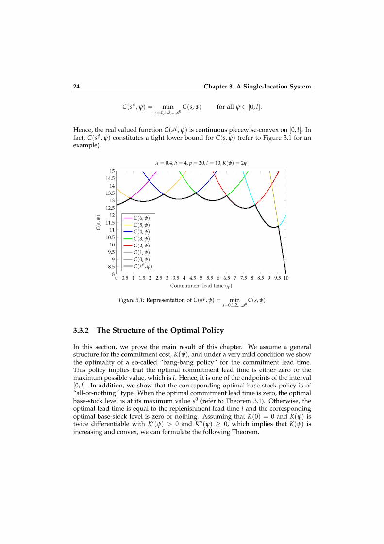
C(sψ, ψ) = mins=0,1,2,...,s0
C(s, ψ) for all ψ ∈ [0, l].
Hence, the real valued function C(sψ, ψ) is continuous piecewise-convex on [0, l]. Infact, C(sψ, ψ) constitutes a tight lower bound for C(s, ψ) (refer to Figure 3.1 for anexample).
0 0.5 1 1.5 2 2.5 3 3.5 4 4.5 5 5.5 6 6.5 7 7.5 8 8.5 9 9.5 108
8.59
9.510
10.511
11.512
12.513
13.514
14.515
Commitment lead time (ψ)
C(s
,ψ)
λ = 0.4, h = 4, p = 20, l = 10, K(ψ) = 2ψ
C(6, ψ)
C(5, ψ)
C(4, ψ)
C(3, ψ)
C(2, ψ)
C(1, ψ)
C(0, ψ)
C(sψ, ψ)
Figure 3.1: Representation of C(sψ, ψ) = mins=0,1,2,...,s0
C(s, ψ)
3.3.2 The Structure of the Optimal Policy
In this section, we prove the main result of this chapter. We assume a generalstructure for the commitment cost, K(ψ), and under a very mild condition we showthe optimality of a so-called ”bang-bang policy” for the commitment lead time.This policy implies that the optimal commitment lead time is either zero or themaximum possible value, which is l. Hence, it is one of the endpoints of the interval[0, l]. In addition, we show that the corresponding optimal base-stock policy is of“all-or-nothing” type. When the optimal commitment lead time is zero, the optimalbase-stock level is at its maximum value s0 (refer to Theorem 3.1). Otherwise, theoptimal lead time is equal to the replenishment lead time l and the correspondingoptimal base-stock level is zero or nothing. Assuming that K(0) = 0 and K(ψ) istwice differentiable with K′(ψ) > 0 and K”(ψ) ≥ 0, which implies that K(ψ) isincreasing and convex, we can formulate the following Theorem.

3.3 Analysis 25
Theorem 3.2 If K′(ψ) − C(s0,0)µX(0)
does not change sign in (0, l), then the optimal com-
mitment lead time policy on [0, l] is a “bang-bang” policy and its corresponding optimalbase-stock policy is of “all-or-nothing” type.
We refer to Appendix 3.6.4 for the proof. The proof of Theorem 3.2 relies onconstructing a monotone lower bound for C(sψ, ψ) on [0, l]. Let CLB(ψ) be the lowerbound. We construct it so that the endpoints of C(sψ, ψ) and CLB(ψ) coincide, i.e.,C(s0, 0) = CLB(0) and C(sl , l) = CLB(l). Therefore, the minimum of C(sψ, ψ) on[0, l] is equal to the minimum of CLB(ψ) on [0, l]. Given that CLB(ψ) is a monotonefunction on a closed interval [0, l], the minimum of C(sψ, ψ) always happens atthe endpoints of [0, l]. Hence, ψ∗ ∈ {0, l}, i.e., the optimal commitment lead timepolicy is a bang-bang policy (refer to Appendix 3.6.4 for the details). In Figure 3.2,we provide two examples for the monotone lower bounds; one where ψ∗ = 0 andanother where ψ∗ = l.
0 1 2 3 4 5 6 7 8 9 1012
16
20
24
28
32
36
40
Commitment lead time (ψ)
Cos
t
λ = 0.4, h = 4, p = 20, l = 10, K(ψ) = 115ψ3 + C(s0,0)
µX(0)ψ
C(sψ, ψ)CLB(ψ)
0 1 2 3 4 5 6 7 8 9 104
5
6
7
8
9
10
11
12
13
Commitment lead time (ψ)
Cos
t
λ = 0.4, h = 4, p = 20, l = 10, K(ψ) = C(s0,0)3µX(0)l3 ψ3
C(sψ, ψ)CLB(ψ)
Figure 3.2: Monotone lower bound CLB(ψ) and C(sψ, ψ) on [0, l]
With Corollary 3.1, we provide sufficient conditions for the optimality of buy-to-stock and buy-to-order strategies.
Corollary 3.1 If K′(ψ) ≥ C(s0,0)µX(0)
in (0, l), then the optimal strategy is the buy-to-stock
strategy and if K′(ψ) ≤ C(s0,0)µX(0)
in (0, l), then it is the buy-to-order strategy.
This corollary implies that the firm either uses the standard base-stock policywithout any commitment lead time (buy-to-stock strategy) or holds no inventoryand uses a commitment lead time of l time units (buy-to-order strategy). For anon-linear commitment cost if the condition in Theorem 3.2 does not hold, then theresult may or may not hold. Theorem 3.2 provides the sufficient condition but not anecessary condition. We provide two numerical examples to clarify this further. We

26 Chapter 3. A Single-location System
use the same parameters in both examples with different commitment costs (pleaserefer to Figure 3.3).
0 1 2 3 4 5 6 7 8 9 1010
12
14
16
18
20
22
Commitment lead time (ψ)
Cos
t
λ = 0.4, h = 4, p = 20, l = 10, K(ψ) = 12ψ2
C(sψ, ψ)CLB(ψ)
0 1 2 3 4 5 6 7 8 9 109
10
11
12
13
14
15
Commitment lead time (ψ)
Cos
t
λ = 0.4, h = 4, p = 20, l = 10, K(ψ) = 15ψ2 + C(s0,0)
5µX(0)ψ
C(sψ, ψ)CLB(ψ)
Figure 3.3: Non-monotone lower bound CLB(ψ) and C(sψ, ψ) on [0, l]
For both examples, we have K′1(ψ) = ψ and K′2(ψ) = 25 ψ + C(s0,0)
5µX(0). Since C(s0,0)
µX(0)=
12.694 = 3.17, there exist ψ1, ψ2 ∈ (0, l) such that for all ψ ∈ [0, ψ1], K′1(ψ1)− C(s0,0)
µX(0)≤
0 and for all ψ ∈ [ψ1, l], K′1(ψ) −C(s0,0)µX(0)
≥ 0. Also, for all ψ ∈ [0, ψ2], K′2(ψ) −C(s0,0)µX(0)
≤ 0 and for all ψ ∈ [ψ2, l], K′2(ψ)−C(s0,0)µX(0)
≥ 0. Therefore, in both cases, for
all ψ ∈ (0, l), K′(ψ)− C(s0,0)µX(0)
is not either non-negative or non-positive. It implies
that the sufficient condition does not hold. However, as it can be seen in Figure 3.3,the bang-bang policy may or may not hold. It does not hold for the first example,while it holds for the second one.
3.4. Linear Commitment Cost
In this section, we consider a linear commitment cost function. We define c as thecommitment cost per time unit and write K(ψ) = cψ. With the following corollary,we prove that the sufficient condition in Theorem 3.2 is satisfied and, therefore, thebang-bang policy is optimal under the linear commitment cost. In addition, weshow that there is a threshold value c0 such that if c > c0, the optimal strategy isthe buy-to-stock strategy and if c ≤ c0, it is the buy-to-order strategy.
Corollary 3.2 If the commitment cost function K(ψ) = cψ, then
1. The optimal commitment lead time policy on [0, l] is a ”bang-bang” policy and itscorresponding optimal base-stock policy is of ”all-or-nothing” type.
3.4 Linear Commitment Cost 27
2. There is a threshold c0 such that if c > c0, then ψ∗ = 0, otherwise, ψ∗ = l. Theexpression for c0 is
c0 =(h + p)
(s0FX(0)(s0)− µX(0)FX(0)(s0 − 1)
)+ p
(µX(0) − s0
)µX(0)
,
where s0 = min{
s ∈N0 : FX(0)(s) ≥p
p+h
}.
The intuition behind this result is that, under the linear commitment cost structure,when a firm has two decisions to make, one on the base-stock level and anotheron the commitment lead time, it has to optimize the total cost by considering thetrade-off of having more/less inventory or longer/shorter commitment lead time.If c ≥ c0, i.e., the unit commitment cost is higher than the threshold, it is cheaper tohold inventory. This is why a solution with no investment on commitment costbut highest investment on inventory is chosen. On the other hand, if c ≤ c0,i.e., the unit commitment cost is lower than the threshold, it is cheaper to havea long commitment lead time. This is why a solution with maximum investmenton commitment cost but no investment on inventory is chosen.
In the rest of this section, we perform sensitivity analysis on the unit commitmentcost threshold, and we illustrate the behavior of C(sψ, ψ) through numericalexamples. Next, we show how to calculate the optimal commitment lead time for afixed base-stock level. In addition, we develop a simple and accurate approximationfor the optimal commitment lead time. Finally, we consider the profit maximizationversion of the problem and determine the conditions on the unit commitment costfor profitability of the buy-to-order strategy.
3.4.1 Sensitivity Analysis on the Unit Commitment Cost Thresh-old
The unit commitment cost threshold c0 plays a critical role in determination of theoptimal strategy. According to Corollary 3.2, c0 is a function of the unit holdingcost h, unit backordering cost p, the mean lead time demand µX(0) and distributionfunction of the lead time demand FX(ψ)(x) for the following pairs of x and ψ;(s0, 0) and (s0 − 1, 0). Since the values of FX(0)(s0) and FX(0)(s0 − 1) also dependon h, p and µX(0) the effect of a change in one of these parameters on c0 is notstraightforward. In Lemma 3.3 we characterize the effect of each parameter on c0.
Lemma 3.3 The unit commitment cost threshold c0 is
1. increasing in the unit holding cost h,
2. increasing in the unit backordering cost p and

28 Chapter 3. A Single-location System
3. decreasing in the mean lead time demand µX(0).
We refer to Appendix 3.6.7 for the proof. According to Lemma 3.3, the constraintc < c0 is likely to hold more often when h and p increase and µX(0) decreases.Hence, the buy-to-order strategy becomes preferable (refer to Corollary 3.2).Inventory management is difficult under high demand uncertainty. Firms may keepexcess inventory to protect against a stock-out situation or they might keep lowinventory to prevent a surplus situation. Under Poisson demand a low mean leadtime demand µX(0) implies a high coefficient of variation ( 1√
µX(0)) and, therefore,
high demand uncertainty. The buy-to-order, i.e., preorder, strategy becomes morebeneficial as the demand uncertainty increases. This holds even for high valuesof the commitment cost. When the unit holding and backordering costs increasethe surplus and stock-out situations become more expensive compared to payinga commitment cost. This is why the preorder strategy becomes more beneficial.Figure 3.4 confirms this conclusion.
0 1 2 3 4 5 6 7 8 9 10 11 12 13 14 15 16 17 18 19 200123456789
101112131415
Unit holding cost (h)
Uni
tco
mm
itm
ent
cost
thre
shol
d(c
0)
p = 15, l = 10
µX(0) = 0.1µX(0) = 1µX(0) = 5µX(0) = 10
0 1 2 3 4 5 6 7 8 9 10 11 12 13 14 15 16 17 18 19 200123456789
101112131415
Unit backordering cost (p)
Uni
tco
mm
itm
ent
cost
thre
shol
d(c
0)
h = 4, l = 10
µX(0) = 0.1µX(0) = 1µX(0) = 5µX(0) = 10
Figure 3.4: Unit Commitment cost threshold as a function of cost factors
Figure 3.4 also illustrates that when the firm has less demand uncertainty, theunit commitment cost threshold is more sensitive to changes in unit holding andbackordering costs. In addition, the unit commitment cost threshold is moresensitive to changes in the unit holding cost compared to changes in the unitbackordering cost.
Consistent with Lemma 3.3, Figure 3.5 shows that the firm prefers the buy-to-order strategy as demand uncertainty increases; inventory related costs outweighthe commitment cost and the preorder strategy becomes preferable even for highvalues of the unit commitment cost.
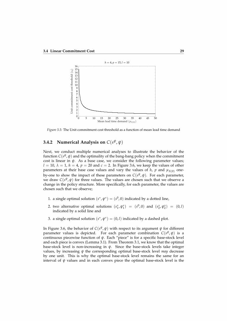
3.4 Linear Commitment Cost 29
0 5 10 15 20 25 30 35 40 45 500123456789
10111213141516
Mean lead time demand (µX(0))
Uni
tco
mm
itm
ent
cost
thre
shol
d(c
0)
h = 4, p = 15, l = 10
Figure 3.5: The Unit commitment cost threshold as a function of mean lead time demand
3.4.2 Numerical Analysis on C(sψ, ψ)
Next, we conduct multiple numerical analyses to illustrate the behavior of thefunction C(sψ, ψ) and the optimality of the bang-bang policy when the commitmentcost is linear in ψ. As a base case, we consider the following parameter values;l = 10, λ = 1, h = 4, p = 20 and c = 2. In Figure 3.6, we keep the values of otherparameters at their base case values and vary the values of h, p and µX(0) one-by-one to show the impact of these parameters on C(sψ, ψ). For each parameter,we draw C(sψ, ψ) for three values. The values are chosen such that we observe achange in the policy structure. More specifically, for each parameter, the values arechosen such that we observe;
1. a single optimal solution (s∗, ψ∗) = (s0, 0) indicated by a dotted line,
2. two alternative optimal solutions (s∗1 , ψ∗1 ) = (s0, 0) and (s∗2 , ψ∗2 ) = (0, l)indicated by a solid line and
3. a single optimal solution (s∗, ψ∗) = (0, l) indicated by a dashed plot.
In Figure 3.6, the behavior of C(sψ, ψ) with respect to its argument ψ for differentparameter values is depicted. For each parameter combination C(sψ, ψ) is acontinuous piecewise function of ψ. Each “piece” is for a specific base-stock leveland each piece is convex (Lemma 3.1). From Theorem 3.1, we know that the optimalbase-stock level is non-increasing in ψ. Since the base-stock levels take integervalues, by increasing ψ the corresponding optimal base-stock level may decreaseby one unit. This is why the optimal base-stock level remains the same for aninterval of ψ values and in each convex piece the optimal base-stock level is the

30 Chapter 3. A Single-location System
0 0.5 1 1.5 2 2.5 3 3.5 4 4.5 5 5.5 6 6.5 7 7.5 8 8.5 9 9.5 10161718192021222324
25262728
Commitment lead time (ψ)
C(s
ψ,ψ
)
λ = 1, p = 20, l = 10, c = 2
h = 5h = 4.1h = 3
0 0.5 1 1.5 2 2.5 3 3.5 4 4.5 5 5.5 6 6.5 7 7.5 8 8.5 9 9.5 1018
19
20
21
22
23
24
25
26
27
28
Commitment lead time (ψ)
C(s
ψ,ψ
)
λ = 1, h = 4, l = 10, c = 2
p = 30p = 21.3p = 15
0 0.5 1 1.5 2 2.5 3 3.5 4 4.5 5 5.5 6 6.5 7 7.5 8 8.5 9 9.5 1016
17
18
19
2021
22
2324
25
26
27
28
Commitment lead time (ψ)
C(s
ψ,ψ
)
h = 4, p = 20, l = 10, c = 2
µX(0) = 11µX(0) = 9.7µX(0) = 8.5
Figure 3.6: Behavior of C(sψ, ψ) based on different values for the problem parameters
same. As soon as the optimal base-stock level decreases (as a response to increasingψ), another convex piece emerges.
Figure 3.6 suggests that for low values of h, ψ∗ is 0 and, hence, the firm followsa buy-to-stock strategy. For sufficiently large h values ψ∗ becomes l and the firmfollows a buy-to-order strategy. This result does not only follow intuitively but alsodirectly from Corollary 3.2. Note that as h → 0, s0 → ∞ and c0 → 0. Hence, c > c0holds and Corollary 3.2 implies the optimality of buy-to-stock strategy.
As the unit backordering cost p increases we observe a similar behavior, i.e., thestrategy changes from buy-to-stock to buy-to-order. In the classical inventorytheory, the effects of h and p are usually opposite. However, in our problem, theireffects are similar. The reason is that the optimality of a policy depends on the valueof c0. As p→ ∞, s0 → ∞ and c0 → ∞. Hence, c0 > c holds and Corollary 3.2 impliesthe optimality of the buy-to-order strategy. Therefore, a buy-to-stock strategy isoptimal for low values of p and a buy-to-order strategy becomes optimal as p getssufficiently large. This implies the same trend in the optimal policy structure as hchanges. Figure 3.6 confirms this conclusion.
As the mean lead time demand µX(0) increases the strategy changes from buy-to-

3.4 Linear Commitment Cost 31
order to buy-to-stock. This is in line with what we observe in the classical inventorytheory. We also observe that as µX(0) increases C(sψ, ψ) becomes a smooth concavefunction. As explained above, in each convex piece in C(sψ, ψ) the optimal base-stock level is the same. When µX(0) increases, the optimal base-stock level becomesmore sensitive to ψ. Hence, the interval of ψ for which a base-stock level remainsoptimal gets shorter, i.e., convex pieces become smaller. As observed in Figure 3.7,when mean lead time demand increases the number of convex pieces increases andfor high mean lead time demand C(sψ, ψ) becomes a smooth concave function.
0 1 2 3 4 5 6 7 8 9 1019
20
21
22
23
24
25
26
Commitment lead time (ψ)
C(s
ψ,ψ
)
µX(0) = 10, h = 4, p = 20, c = 2
0 1 2 3 4 5 6 7 8 9 1025
27
29
31
33
35
37
3941
43
45
47
49
Commitment lead time (ψ)
C(s
ψ,ψ
)
µX(0) = 20, h = 4, p = 20, c = 2
0 1 2 3 4 5 6 7 8 9 1060
80
100
120
140
160
180
200
220
Commitment lead time (ψ)
C(s
ψ,ψ
)
µX(0) = 100, h = 4, p = 20, c = 2
Figure 3.7: Behavior of C(sψ, ψ) for different values of µX(0)
3.4.3 Optimal Commitment Lead Time for a Given Base-stockLevel
As we already noted the commitment lead time and base-stock level are dependentdecision variables. If the firm relies on a vendor-managed inventory policy, whereinventory is controlled by the supplier, the only decision variable that the firm canoptimize is the commitment lead time. In this section, we assume that the base-stock level is already set and we determine the expression for the corresponding
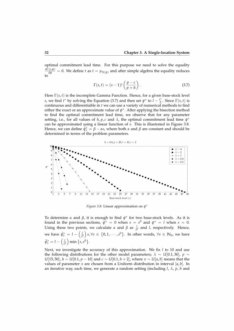
32 Chapter 3. A Single-location System
optimal commitment lead time. For this purpose we need to solve the equalitydC(s,ψ)
dψ = 0. We define t as t = µX(ψ) and after simple algebra the equality reducesto
Γ(s, t) = (s− 1)!(
p− cp + h
). (3.7)
Here Γ(s, t) is the incomplete Gamma Function. Hence, for a given base-stock levels, we find t∗ by solving the Equation (3.7) and then set ψ∗ to l − t∗
λ . Since Γ(s, t) iscontinuous and differentiable in t we can use a variety of numerical methods to findeither the exact or an approximate value of ψ∗. After applying the bisection methodto find the optimal commitment lead time, we observe that for any parametersetting, i.e., for all values of h, p, c and λ, the optimal commitment lead time ψ∗
can be approximated using a linear function of s. This is illustrated in Figure 3.8.Hence, we can define ψ∗s = β− αs, where both α and β are constant and should bedetermined in terms of the problem parameters.
1 3 5 7 9 11 13 15 17 19 21 23 25 27 29 31 33 35 37 39 41 43 45 47 490
1
2
3
4
5
6
7
8
9
10
Base-stock level (s)
ψ∗
h = 0.4, p = 20, l = 10, c = 2
λ = 4λ = 2λ = 1λ = 0.4λ = 0.2
Figure 3.8: Linear approximation on ψ∗
To determine α and β, it is enough to find ψ∗ for two base-stock levels. As it isfound in the previous sections, ψ∗ = 0 when s = s0 and ψ∗ = l when s = 0.Using these two points, we calculate α and β as l
s0 and l, respectively. Hence,
we have ψ∗s = l −(
ls0
)s, ∀s ∈
{0, 1, · · · , s0}. In other words, ∀s ∈ N0, we have
ψ∗s = l −(
ls0
)min
{s, s0}.
Next, we investigate the accuracy of this approximation. We fix l to 10 and usethe following distributions for the other model parameters; λ ∼ U[0.1, 30], p ∼U[15, 50], h ∼ U[0.1, p− 10] and c ∼ U[0.1, h + 2], where x ∼ U[a, b] means that thevalues of parameter x are chosen from a Uniform distribution in interval [a, b]. Inan iterative way, each time, we generate a random setting (including l, λ, p, h and

3.4 Linear Commitment Cost 33
c) and calculate ψ∗s and ψ∗s . We consider 8000 parameter combinations and for eachparameter combination i, we consider the base-stock values from 1 to s0
i − 1, wheres0
i is the the maximum value the base-stock level can take under the parametercombination i. We define εi,s as the approximation percentage error for parametercombination i and the base-stock level s ∈
{1, 2, · · · , s0
i − 1}
. We calculate εi,s asfollows:
εi,s =C(s, ψ∗s )− C(s, ψ∗s )
C(s, ψ∗s )× 100 s = 1, 2, · · · , s0
i − 1, i = 1, 2, · · · , 8000. (3.8)
We calculate the mean percentage error for each combination i as follows;
Ei =
1s0
i − 1
s0i −1
∑s=1
εi,s
, i = 1, 2, · · · , 8000. (3.9)
In Figure 3.9, we plot the cumulative distribution of the mean percentage error. Forthis purpose, we define E as a discrete uniform random variable such that P(E =
Ei) = 18000 , ∀i ∈ {1, 2, · · · , 8000}. The figure suggests that the mean percentage
error is below 5% in approximately 90% of the cases.
0 1 2 3 4 5 6 7 8 9 10 11 12 13 14 15 16 17 18 19 200
0.1
0.2
0.3
0.4
0.5
0.6
0.7
0.8
0.9
1
x
P(E≤
x)
λ ∼ U[0.5, 30], p ∼ U[15, 50], h ∼ U[0.1, p− 10], c ∼ U[0.5, h + 2], l = 10, n = 8000
Figure 3.9: The cumulative distribution function of the mean percentage error
3.4.4 Profitability of the Optimal Policy
In the previous sections, we study the cost minimization problem mins∈N0,ψ∈[0,l]
C(s, ψ).
We prove that the optimal strategy is either buy-to-order or buy-to-stock. Inthis section, we concentrate on the buy-to-order strategy and analyze the average

34 Chapter 3. A Single-location System
total profit. If the firm follows the buy-to-order strategy, the only positive costcomponent is the commitment cost cl. Define v as the unit selling price and Θ asthe average total profit of the firm per time unit. Then we formulate the long-runaverage profit of the firm under the buy-to-order (BTO) strategy as follows;
ΘBTO = λv− λcl = λ(v− cl).
The long-run average profit of the firm is non-negative when c < vl . In addition, the
optimality of the buy-to-order strategy requires c ≤ c0. Hence, the unit commitmentcost should satisfy the following inequality
c < min{
c0,vl
}.
In Figure 3.10, we consider the unit commitment cost and the mean lead timedemand and determine the region where the buy-to-order strategy is profitable.
c0
← c = vl
BTS
BTO
BTO
Profitable
Non-profitable
Mean lead time demand (µX(0))
Uni
tco
mm
itm
ent
cost
(c)
Figure 3.10: Optimal strategies
Figure 3.10 helps managers in making strategy decisions when, in addition to theinventory-related and commitment costs, the revenue from selling the product isconsidered. Figure 3.10 suggests that profitability of the buy-to-order strategydepends on the value of c and, although it is cost optimal, the firm should notfollow this strategy for high values of c as it is non-profitable. When the optimalstrategy is the buy-to-stock strategy, the unit commitment cost does not play a rolein the total profit of the firm.
3.5. Conclusion
In this chapter, we investigated the impact of the commitment cost on thereplenishment strategy of a firm under continuous-review setting. The firm facesa Poisson customer demand and uses a preorder strategy which requires that
3.5 Conclusion 35
customers place their orders ahead of the actual need based on a pre-determinedtime window called commitment lead time. The firm pays a commitment cost whichis strictly increasing and convex in the length of the commitment lead time. Thefirm uses a base-stock replenishment policy with a deterministic lead time. Thefirm’s objective is to find the commitment lead time and the base-stock level whichminimize the total average cost consisting of inventory holding, backordering andcommitment costs. This is a non-linear mixed-integer optimization problem. Wehave a continuous commitment lead time and a discrete base-stock level as ourdecision variables and they are dependent on each other.
We proved the convexity of the average cost function in each decision variable.We showed that the optimal base-stock level is non-increasing in the length of thecommitment lead time. The average cost as a function of a commitment lead timeand the corresponding optimal base-stock level served as a continuous piecewise-convex lower bound on the original average cost function. We constructed anothermonotone lower bound on this piecewise-convex lower bound. This monotonelower bound implied the optimality of the bang-bang policy for the commitmentlead time. Under this policy the commitment lead time is either zero or themaximum possible value, which is the replenishment lead time. In addition, weshowed that the corresponding optimal base-stock policy is of all-or-nothing type.Hence, the optimal base-stock level is either zero or the solution of the well-knownNewsvendor problem with complete replenishment lead time.
The optimality of the bang-bang policy holds for general commitment coststructures under a very mild condition. As a specific case, we studied a linearcommitment cost. For this case, we found a unit commitment cost threshold whichdictates the optimality of either a buy-to-order or a buy-to-stock strategy. Morespecifically, we showed that when the unit commitment cost is less than the unitcommitment cost threshold, the optimal ordering strategy is a buy-to-order strategy(the optimal commitment lead time is equal to replenishment lead time and theoptimal base-stock level is zero) and when the unit commitment cost is more thanthe unit commitment cost threshold, the optimal strategy is a pure buy-to-stockstrategy (the optimal commitment lead time is zero and optimal base-stock levelis non-zero). Moreover, we showed that the unit commitment cost threshold isincreasing in the unit holding and backordering costs and decreasing in the meanlead time demand. For a given base-stock level, we developed a simple and accurateapproximation for the corresponding optimal commitment lead time. Finally, wedetermined the conditions on the unit commitment cost for profitability of the buy-to-order strategy.
In this chapter, we studied a system with a single location and a single item witha cost minimization objective. A natural extension is to replace the backorderingcost with a service level and/or waiting time constraints and check whether theoptimality of a bang-bang policy remain. Another extension is to consider a systemwhere each customer places an order for a product which needs to be assembled

36 Chapter 3. A Single-location System
from multiple components with different replenishment lead times. Then, the firmneeds to find the optimal replenishment policy for each component and also theoptimal commitment lead time. More general assembly structures can also beanalyzed.
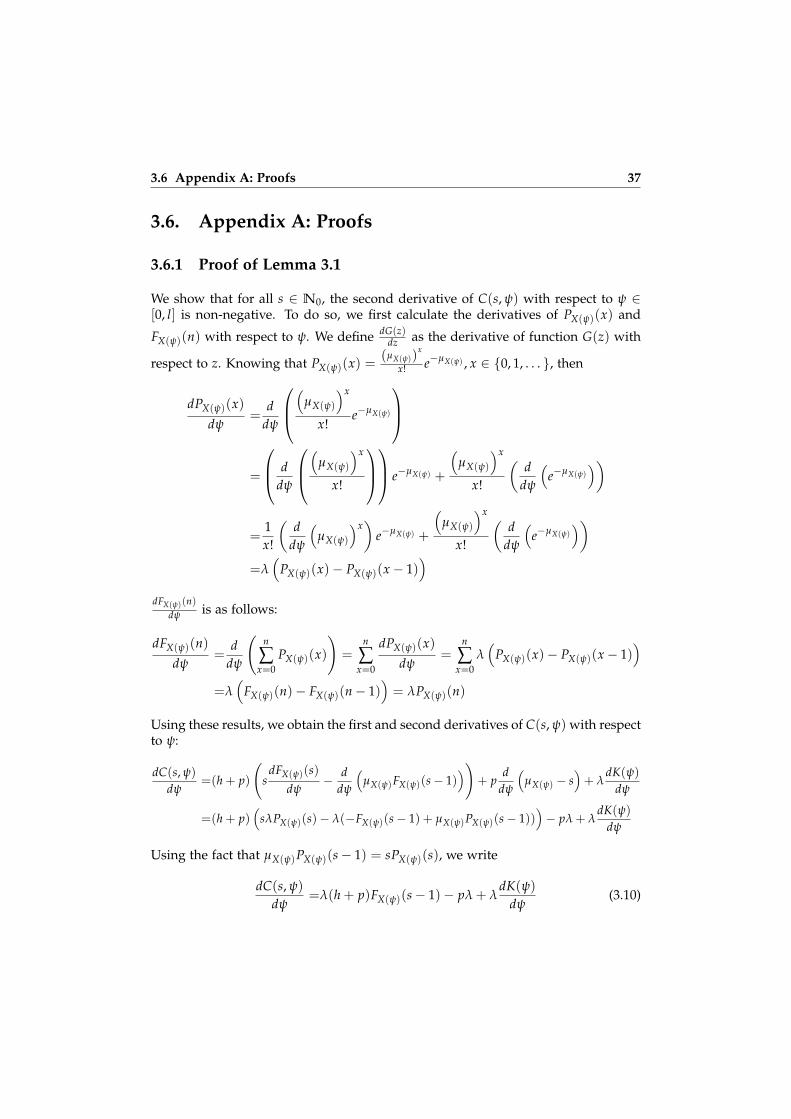
3.6 Appendix A: Proofs 37
3.6. Appendix A: Proofs
3.6.1 Proof of Lemma 3.1
We show that for all s ∈ N0, the second derivative of C(s, ψ) with respect to ψ ∈[0, l] is non-negative. To do so, we first calculate the derivatives of PX(ψ)(x) and
FX(ψ)(n) with respect to ψ. We define dG(z)dz as the derivative of function G(z) with
respect to z. Knowing that PX(ψ)(x) = (µX(ψ))x
x! e−µX(ψ) , x ∈ {0, 1, . . . }, then
dPX(ψ)(x)dψ
=d
dψ
(
µX(ψ)
)x
x!e−µX(ψ)
=
ddψ
(
µX(ψ)
)x
x!
e−µX(ψ) +
(µX(ψ)
)x
x!
(d
dψ
(e−µX(ψ)
))
=1x!
(d
dψ
(µX(ψ)
)x)
e−µX(ψ) +
(µX(ψ)
)x
x!
(d
dψ
(e−µX(ψ)
))=λ
(PX(ψ)(x)− PX(ψ)(x− 1)
)dFX(ψ)(n)
dψ is as follows:
dFX(ψ)(n)dψ
=d
dψ
(n
∑x=0
PX(ψ)(x)
)=
n
∑x=0
dPX(ψ)(x)dψ
=n
∑x=0
λ(
PX(ψ)(x)− PX(ψ)(x− 1))
=λ(
FX(ψ)(n)− FX(ψ)(n− 1))= λPX(ψ)(n)
Using these results, we obtain the first and second derivatives of C(s, ψ) with respectto ψ:
dC(s, ψ)
dψ=(h + p)
(s
dFX(ψ)(s)dψ
− ddψ
(µX(ψ)FX(ψ)(s− 1)
))+ p
ddψ
(µX(ψ) − s
)+ λ
dK(ψ)dψ
=(h + p)(
sλPX(ψ)(s)− λ(−FX(ψ)(s− 1) + µX(ψ)PX(ψ)(s− 1)))− pλ + λ
dK(ψ)dψ
Using the fact that µX(ψ)PX(ψ)(s− 1) = sPX(ψ)(s), we write
dC(s, ψ)
dψ=λ(h + p)FX(ψ)(s− 1)− pλ + λ
dK(ψ)dψ
(3.10)

38 Chapter 3. A Single-location System
and
d2C(s, ψ)
dψ2 =λ2(h + p)PX(ψ)(s− 1) + λd2K(ψ)
dψ2 (3.11)
Since ∀s ∈ N0 and ψ ∈ [0, l], we have d2K(ψ)dψ2 ≥ 0 and PX(ψ)(s − 1) ≥ 0, then
d2C(s,ψ)dψ2 ≥ 0. It means that for all s ∈N0, then C(s, ψ) is convex with respect to ψ.
3.6.2 Proof of Lemma 3.2
The concept of convexity for a real valued function on a discrete domain is notcommon. According to van Houtum and Kranenburg (2015) this concept can bedefined as follows.
Definition 3.1 Let f(x) be a function on Z and x0 ∈ Z, then f(x) is convex for x ≥ x0if
∆2 f (x) = ∆ f (x + 1)− ∆ f (x) ≥ 0, x ≥ x0
where ∆ f (x) = f (x + 1)− f (x).
The function C(s, ψ) is convex in s ∈ N0 if for all ψ ∈ [0, l] we have ∆2s C(s, ψ) ≥ 0,
where ∆2s C(s, ψ) is defined as follows:
∆2s C(s, ψ) =∆sC(s + 1, ψ)− ∆sC(s, ψ)
= (C(s + 2, ψ)− C(s + 1, ψ))− (C(s + 1, ψ)− C(s, ψ))
=C(s + 2, ψ)− 2C(s + 1, ψ) + C(s, ψ).
Next, we determine the expressions for C(s + 1, ψ) and C(s + 2, ψ).
C(s + 1, ψ) =(h + p)((s + 1)FX(ψ)(s + 1)− µX(ψ)FX(ψ)(s)) + p(µX(ψ) − (s + 1)) + λK(ψ)
=(h + p)(sFX(ψ)(s + 1) + FX(ψ)(s + 1)− µX(ψ)FX(ψ)(s− 1)
− µX(ψ)PX(ψ)(s)) + p(
µX(ψ) − s)− p + λK(ψ)
=(h + p)(sFX(ψ)(s) + sPX(ψ)(s + 1) + FX(ψ)(s + 1)− µX(ψ)FX(ψ)(s− 1)
− µX(ψ)PX(ψ)(s)) + p(
µX(ψ) − s)− p + λK(ψ)
From the Poisson probability mass function we know µX(ψ)PX(ψ)(s) = (s +

3.6 Appendix A: Proofs 39
1)PX(ψ)(s + 1). Then,
C(s + 1, ψ) =(h + p)(sFX(ψ)(s) + sPX(ψ)(s + 1) + (PX(ψ)(s + 1) + FX(ψ)(s))
− µX(ψ)FX(ψ)(s− 1)− µX(ψ)PX(ψ)(s)) + p(
µX(ψ) − s)− p + λK(ψ)
=(h + p)FX(ψ)(s)− p + (h + p)(sFX(ψ)(s)− µX(ψ)FX(ψ)(s− 1))
+ p(
µX(ψ) − s)+ λK(ψ)
=(h + p)FX(ψ)(s)− p + C(s, ψ)
Using the last expression, we write C(s + 2, ψ) as
C(s + 2, ψ) =(h + p)FX(ψ)(s + 1)− p + C(s + 1, ψ)
=(h + p)FX(ψ)(s + 1)− p + (h + p)FX(ψ)(s)− p + C(s, ψ)
=(h + p)(FX(ψ)(s + 1) + FX(ψ)(s))− 2p + C(s, ψ)
Using these expressions, we write ∆2s C(s, ψ) as
∆2s C(s, ψ) =(h + p)(FX(ψ)(s + 1) + FX(ψ)(s))− 2p + C(s, ψ)
− 2((h + p)FX(ψ)(s)− p + C(s, ψ)) + C(s, ψ)
=(h + p)(FX(ψ)(s + 1)− FX(ψ)(s))
=(h + p)PX(ψ)(s + 1)
Since ∀s ∈ N0 and ψ ∈ [0, l], PX(ψ)(s + 1) ≥ 0, then ∆2s C(s, ψ) ≥ 0. Hence, ∀ψ ∈
[0, l], C(s, ψ) is convex with respect to s.
3.6.3 Proof of Theorem 3.1
We use the following Lemma in proving the result.
Lemma 3.4 Let FX(ψ)(s) be the Poisson cumulative distribution function of X(ψ) withmean µX(ψ), then,
1. for all s ∈N0 and λ ≥ 0, FX(ψ)(s) is increasing in ψ.
2. for all ψ ∈ [0, l], FX(ψ)(s) is increasing in s.
Proof: For all s ∈ N0, FX(ψ)(s) is a continuous and differentiable function withrespect to ψ, then from the proof of Lemma 3.1 in Appendix 3.6.1, we havedFX(ψ)(s)
dψ = λPX(ψ)(s). For each s ∈ N0 and ψ ∈ [0, l], PX(ψ)(s) ≥ 0. Then, forall λ ≥ 0, FX(ψ)(s) is increasing in ψ.

40 Chapter 3. A Single-location System
For all ψ ∈ [0, l], FX(ψ)(s) is a discrete function with respect to s, then by calculatingthe first order forward difference, we have;
∆sFX(ψ)(s) = FX(ψ)(s)− FX(ψ)(s− 1) = PX(ψ)(s) ≥ 0.
Then, FX(ψ)(s) is increasing in s. Define S as the set all optimal base-stock levels∀ψ ∈ [0, l]. We have
S =
{s ∈N0 : FX(ψ)(s− 1) <
ph + p
≤ FX(ψ)(s), ψ ∈ [0, l]}
Let s0 be the base-stock level corresponding to ψ = 0. It means that
FX(0)(s0 − 1) <
ph + p
≤ FX(0)(s0)
Since FX(ψ)(s) is increasing and continuous in ψ (Lemma 3.4), then by increasingψ, both functions FX(ψ)(s− 1) and FX(ψ)(s) increase until a ψs0,s0−1 > 0 such thatFX(ψs0,s0−1)
(s0 − 1) = ph+p . Hence, for 0 ≤ ψ < ψs0,s0−1 and s∗ = s0, Inequality (3.6)
holds. Since FX(ψ)(s) is increasing in s (Lemma 3.4), we can write,
FX(ψs0,s0−1)(s0 − 2) <
ph + p
≤ FX(ψs0,s0−1)(s0 − 1) (3.12)
In a similar way, by increasing ψ, we can find ψs0−1,s0−2 such that ψs0−1,s0−2 >
ψs0,s0−1 and FX(ψs0,s0−1)(s0 − 2) = p
h+p . Hence, for ψs0,s0−1 ≤ ψ < ψs0−1,s0−2 and
s∗ = s0 − 1, Inequality (3.6) holds. Continuing this process, we find S = {s0, s0 −1, ..., 2, 1, 0} as corresponding to each s∗ ∈ S, there is a subinterval Ψs, Ψs ⊂ [0, l]such that,
Ψs =
[0, ψs0,s0−1), if s∗ = s0
[ψs∗+1,s∗ , ψs∗ ,s∗−1), if s∗ = 1, 2, 3, ..., s0 − 1[ψ1,0, l], if s∗ = 0
From the last expression, it is clear that s∗ depends on ψ and s∗ is non-increasing inψ.
3.6.4 Proof of Theorem 3.2
We need an additional result to prove this theorem. We define C(s, ψ) on [0, l] asfollows;
C(s, ψ) = C(s, ψ)− λK(ψ) (3.13)
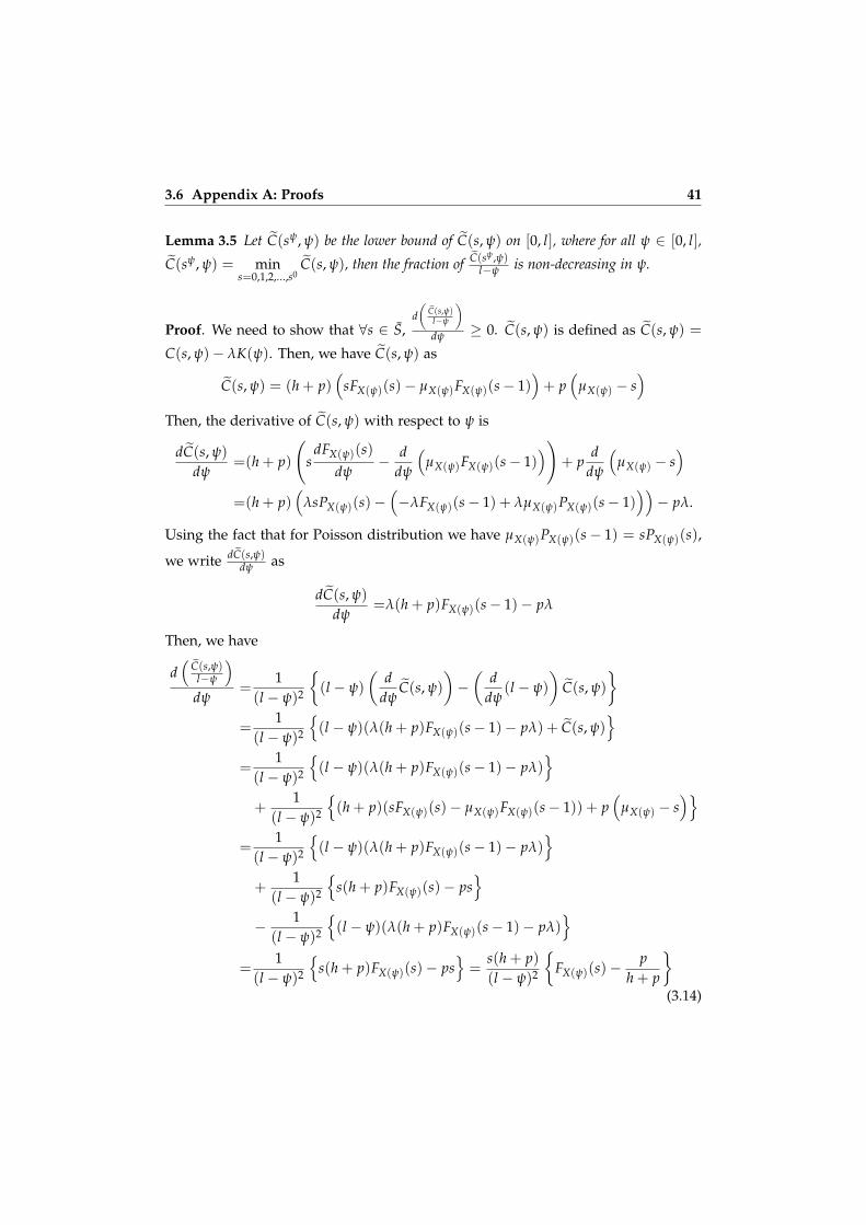
3.6 Appendix A: Proofs 41
Lemma 3.5 Let C(sψ, ψ) be the lower bound of C(s, ψ) on [0, l], where for all ψ ∈ [0, l],
C(sψ, ψ) = mins=0,1,2,...,s0
C(s, ψ), then the fraction of C(sψ ,ψ)l−ψ is non-decreasing in ψ.
Proof. We need to show that ∀s ∈ S,d(
C(s,ψ)l−ψ
)dψ ≥ 0. C(s, ψ) is defined as C(s, ψ) =
C(s, ψ)− λK(ψ). Then, we have C(s, ψ) as
C(s, ψ) = (h + p)(
sFX(ψ)(s)− µX(ψ)FX(ψ)(s− 1))+ p
(µX(ψ) − s
)Then, the derivative of C(s, ψ) with respect to ψ is
dC(s, ψ)
dψ=(h + p)
(s
dFX(ψ)(s)dψ
− ddψ
(µX(ψ)FX(ψ)(s− 1)
))+ p
ddψ
(µX(ψ) − s
)=(h + p)
(λsPX(ψ)(s)−
(−λFX(ψ)(s− 1) + λµX(ψ)PX(ψ)(s− 1)
))− pλ.
Using the fact that for Poisson distribution we have µX(ψ)PX(ψ)(s− 1) = sPX(ψ)(s),
we write dC(s,ψ)dψ as
dC(s, ψ)
dψ=λ(h + p)FX(ψ)(s− 1)− pλ
Then, we have
d(
C(s,ψ)l−ψ
)dψ
=1
(l − ψ)2
{(l − ψ)
(d
dψC(s, ψ)
)−(
ddψ
(l − ψ)
)C(s, ψ)
}=
1(l − ψ)2
{(l − ψ)(λ(h + p)FX(ψ)(s− 1)− pλ) + C(s, ψ)
}=
1(l − ψ)2
{(l − ψ)(λ(h + p)FX(ψ)(s− 1)− pλ)
}+
1(l − ψ)2
{(h + p)(sFX(ψ)(s)− µX(ψ)FX(ψ)(s− 1)) + p
(µX(ψ) − s
)}=
1(l − ψ)2
{(l − ψ)(λ(h + p)FX(ψ)(s− 1)− pλ)
}+
1(l − ψ)2
{s(h + p)FX(ψ)(s)− ps
}− 1
(l − ψ)2
{(l − ψ)(λ(h + p)FX(ψ)(s− 1)− pλ)
}=
1(l − ψ)2
{s(h + p)FX(ψ)(s)− ps
}=
s(h + p)(l − ψ)2
{FX(ψ)(s)−
ph + p
}(3.14)
42 Chapter 3. A Single-location System
d(
C(s,ψ)l−ψ
)dψ
=s(h + p)(l − ψ)2
{FX(ψ)(s)−
ph + p
}(3.15)
Since we subtract K(ψ) from C(s, ψ) and K(ψ) does not depend on s, we have thesame set S as we had before for the lower bound of C(s, ψ). Also, from Inequality
(3.6) we know FX(ψ)(s) ≥p
h+p . Then for all s ∈ S,d(
C(s,ψ)l−ψ
)dψ ≥ 0.
From Lemma 3.5 we know that C(sψ ,ψ)l−ψ is non-decreasing in ψ on closed interval
[0, l]. Then, The fraction C(sψ ,ψ)l−ψ has its minimum value at the beginning of the
interval [0, l]. Hence, for all ψ ∈ [0, l] we have C(sψ ,ψ)l−ψ ≥ C(s0,0)
l−0 . Since for allψ ∈ [0, l], we have l − ψ ≥ 0, then,
C(sψ, ψ) ≥ C(s0, 0)l
(l − ψ) (3.16)
By adding λK(ψ) to the both sides of (3.16), we have
C(sψ, ψ) + λK(ψ) ≥ C(s0, 0)l
(l − ψ) + λK(ψ) (3.17)
We know that K(0) = 0. Also, from Expression (3.15), we have C(sψ, ψ) =
C(sψ, ψ)− λK(ψ). Then, C(s0, 0) = C(s0, 0) and we can rewrite Expression (3.17) asfollows.
C(sψ, ψ) ≥ C(s0, 0)l
(l − ψ) + λK(ψ) (3.18)
Let CLB(ψ) = C(s0,0)l (l − ψ) + λK(ψ). Then, CLB(ψ) is a lower bound for C(sψ, ψ)
on [0, l]. Since C(s0, 0) = CLB(0) and C(sl , l) = CLB(l), then C(sψ, ψ) and CLB(ψ)coincide at the endpoints of the interval [0, l]. Now, we want to show that CLB(ψ) isa monotone function on [0, l]. To do this, we show that for all ψ ∈ [0, l], dCLB(ψ)
dψ 6= 0.By taking the first derivative of CLB(ψ) with respect to ψ we have
dCLB(ψ)
dψ=
C(s0, 0)l
d(l − ψ)
dψ+ λ
dK(ψ)dψ
= −C(s0, 0)l
+ λK′(ψ) = λ
(K′(ψ)− C(s0, 0)
µX(0)
)(3.19)
For all ψ ∈ (0, l), we have either K′(ψ)− C(s0,0)µX(0)
≥ 0, or K′(ψ)− C(s0,0)µX(0)
≤ 0. It means
that CLB(ψ) is a monotone lower bound for C(sψ, ψ) on [0, l]. Then, the minimum

3.6 Appendix A: Proofs 43
of C(sψ, ψ) on [0, l] is equal to the minimum of CLB(ψ) on [0, l]. Since CLB(ψ) isa monotone function on [0, l] and [0, l] is a closed interval, then the minimum ofC(sψ, ψ) always happens at the endpoints of [0, l]. Then, ψ∗ ∈ {0, l}. The optimalityof “all-or-nothing” base-stock policy follows directly from Theorem 3.1.
3.6.5 Proof of Corollary 3.1
From Expression (3.19), it is obvious that when K′(ψ) ≥ C(s0,0)µX(0)
, then CLB(ψ) is a
non-decreasing function in ψ and its minimum occurs at zero, i.e., ψ∗ = 0. And
when K′(ψ)(ψ) ≤ C(s0,0)µX(0)
, then CLB(ψ) is a non-increasing function in ψ and its
minimum occurs at l, i.e., ψ∗ = l.
3.6.6 Proof of Corollary 3.2
1. This part follows directly from Theorem 3.2. When K(ψ) = cψ, then CLB(ψ) =
C(s0, 0) +(
cλ− C(s0,0)l
)ψ which is a straight line. Then, ∀ψ ∈ [0, l], CLB(ψ) is
a monotone function. Also, CLB(0) = C(s0, 0) and CLB(l) = C(sl , l). Then theoptimal ψ on [0, l] is either zero or l.
2. From CLB(ψ) = C(s0, 0)+(
cλ− C(s0,0)l
)ψ, when cλ− C(s0,0)
l > 0, then CLB(ψ)
is increasing in ψ and CLB(0) is its minimum value on [0, l]. Otherwise, CLB(ψ)is decreasing in ψ and CLB(l) is its minimum value on [0, l]. Also, when
cλ− C(s0,0)l = 0, then CLB(ψ) = C(s0, 0). So, CLB(ψ) is a constant function on
[0, l] and the optimal commitment lead time is 0 and l.
3.6.7 Proof of Lemma 3.3
For each h, p and µX(0) 6= 0, c0 is continuous and differentiable.
1. The first derivative of c0 with respect to h is
∂c0
∂h=
s0
µX(0)FX(0)(s
0)− FX(0)(s0 − 1) =
s0
µX(0)
(FX(0)(s
0)−µX(0)
s0 FX(0)(s0 − 1)
)(3.20)
Now we need to show that FX(0)(s0) ≥ µX(0)s0 FX(0)(s0 − 1). For x = 0, 1, 2, , s0 −
1 and µX(0) ≥ 0, we can write s0 ≥ x + 1. Then, 1s0 ≤ 1
x+1 . We can multiply

44 Chapter 3. A Single-location System
both sides of the last inequality by (µX(0))x+1
x! e−µX(0) ≥ 0, then
1s0
(
µX(0)
)x+1
x!e−µX(0)
≤ 1x + 1
(
µX(0)
)x+1
x!e−µX(0)
=
(µX(0)
)x+1
(x + 1)!e−µX(0)
Using this inequality, we write
µX(0)
s0 FX(0)(s0 − 1) =
µX(0)
s0
s0−1
∑x=0
(µX(0)
)x
x!e−µX(0) =
s0−1
∑x=0
(µX(0)
)x+1
s0x!e−µX(0)
≤s0−1
∑x=0
(µX(0)
)x+1
(x + 1)x!e−µX(0) =
s0−1
∑x=0
(µX(0)
)x+1
(x + 1)!e−µX(0)
=s0
∑x=1
(µX(0)
)x
x!e−µX(0) =
s0
∑x=0
(µX(0)
)x
x!e−µX(0) − PX(0)(0)
= FX(0)(s0)− PX(0)(0) < FX(0)(s
0)
Hence,µX(0)
s0 FX(0)(s0 − 1) < FX(0)(s0). Then, from Expression (3.20), we have∂c0∂h > 0. As a result, c0 is increasing in h.
2. The first derivative of c0 with respect to p is
∂c0
∂p=
s0
µX(0)FX(0)(s
0)− FX(0)(s0 − 1) + 1− s0
µX(0)
=s0
µX(0)FX(0)(s
0 − 1) +s0
µX(0)PX(0)(s
0)− FX(0)(s0 − 1) + 1− s0
µX(0)
=− s0
µX(0)(1− FX(0)(s
0 − 1)) + (1− FX(0)(s0 − 1)) +
s0
µX(0)PX(0)(s
0)
=− s0
µX(0)
∞
∑x=s0
(µX(0)
)x
x!e−µX(0) +
∞
∑x=s0
(µX(0)
)x
x!e−µX(0) +
s0
µX(0)PX(0)(s
0)
=− s0
µX(0)
∞
∑x=s0
(µX(0)
)x
x!e−µX(0) − PX(0)(s
0)
+∞
∑x=s0
(µX(0)
)x
x!e−µX(0)
=∞
∑x=s0
(µX(0)
)x
x!e−µX(0)
(1− s0
x + 1
)

3.6 Appendix A: Proofs 45
Since x ≥ s0 we have x + 1 > s0. Hence, s0
x+1 < 1. Thus,(
1− s0
x+1
)> 0. As a
result, we have ∂c0∂p > 0, implying that c0 is increasing in p.
3. The first derivative of c0 with respect to µX(0) is
∂c0
∂µX(0)=s0(h + p)
d(
FX(0)(s0)
µX(0)
)dµX(0)
− (h + p)
(dFX(0)(s0 − 1)
dµX(0)
)−
d(
ps0
µX(0)
)dµX(0)
=s0(h + p)
µX(0)
(dFX(0)(s
0)
dµX(0)
)− FX(0)(s0)(
µX(0)
)2
− (h + p)dFX(0)(s0 − 1)
dµX(0)
−
−ps0(µX(0)
)2
Using the equalities
dFX(0)(s0)
dµX(0)= −PX(0)(s0) and
dFX(0)(s0−1)
dµX(0)= −PX(0)(s0 − 1)
we write
= s0(h + p)
−µX(0)PX(0)(s0)− FX(0)(s0)(µX(0)
)2
+ (h + p)PX(0)(s0 − 1) +
ps0(µX(0)
)2
=s0(
µX(0)
)2
−µX(0)(h + p)PX(0)(s0)− (h + p)FX(0)(s
0) +
(µX(0)
)2
s0 (h + p)PX(0)(s0 − 1) + p
=
s0(µX(0)
)2
(−µX(0)(h + p)PX(0)(s
0)− (h + p)FX(0)(s0) + µX(0)(h + p)
(µX(0)
s0 PX(0)(s0 − 1)
)+ p
)
For Poisson probability distribution we know that µX(0)PX(0)(s0 − 1) =
s0PX(0)(s0). Then, the last expression reduces to
∂c0
∂µX(0)= − s0(h + p)(
µX(0)
)2
(FX(0)(s
0)− pp + h
)
Since s0 ∈ S, then FX(0)(s0) ≥ pp+h and ∂c0
∂µX(0)≤ 0. As a result, c0 is decreasing
in µX(0).
46 Chapter 3. A Single-location System
3.7. Appendix B: Compound Poisson Demand
We extend our study by assuming compound Poisson customer demand. Bydefinition, compound Poisson demand means that the size of customer demandX is also a stochastic variable. It is independent of other customer demands andthe distribution of the customer arrival process. Similar to our previous assumption,we assume that the customer arrival process is a Poisson process with parameter λ.Then the number of customersN (ψ) in a time interval of length l−ψ (i.e., lead timedemand) has a Poisson distribution with mean µN (ψ). We define PN (ψ)(n) as theprobability that the random variable N (ψ) takes the value n when the commitmentlead time is ψ. We have
PN (ψ)(n) =(µN (ψ))
n
n!e−µN (ψ) , n = 0, 1, 2, . . . (3.21)
Let fx be the probability that a customer demands x units, i.e., the probability thatX takes the value x = 1, 2, . . . units. Assume that the mean demand size is µ.When f1 = 1, the demand process is a pure Poisson process. Then total demandin a given interval is equal to the number of customer arrivals. For handling thegeneral case with varying demand sizes, we define f n
x as the probability that n =1, 2, . . . customers demand x units. Since customer demand with the size of zerois not rational, then without loss of generality we assume that f0 = 0 (Feeneyand Sherbrooke (1966)). Knowing that f0 = 0 and f 1
x = fx, f nx can be calculated
recursively as follows (see page 79 in Axsater (2006)):
f nx =
x−1
∑i=n−1
f n−1i fx−i, n = 2, 3, . . . (3.22)
We define D(ψ) as a random variable representing the total demand in the timeinterval l − ψ. In addition, we define PD(ψ)(x) as the probability that D(ψ) takesthe value x when the commitment lead time is ψ. Using Expressions (3.21) and(3.22), we write PD(ψ)(x) as follows:
PD(ψ)(x) =
{PN (ψ)(0) x = 0
∑xn=1 f n
x PN (ψ)(n) x = 1, 2, . . . ,(3.23)
Then, the cumulative distribution function of D(ψ) is calculated as FD(ψ)(s) =
∑sx=0 PD(ψ)(x).
Based on these definitions, the long-run average total cost C(s, ψ) consisting of

3.7 Appendix B: Compound Poisson Demand 47
holding, backordering and commitment costs can be calculated as follows:
C(s, ψ) =hE{[s−D(ψ)]+
}+ pE
{[D(ψ)− s]+
}+ µλK(ψ)
=hs
∑x=0
(s− x)PD(ψ)(x) + p∞
∑x=s+1
(x− s)PD(ψ)(x) + µλK(ψ)
=hss
∑x=0
PD(ψ)(x)− hs
∑x=0
xPD(ψ)(x) + p∞
∑x=s+1
xPD(ψ)(x)
− ps∞
∑x=s+1
PD(ψ)(x) + µλK(ψ)
=hsFD(ψ)(s)− hs
∑x=0
xPD(ψ)(x) + p
(E{D(ψ)} −
s
∑x=0
xPD(ψ)(x)
)− ps
(1− FD(ψ)(s)
)+ µλK(ψ)
=(h + p)
(sFD(ψ)(s)−
s
∑x=0
xPD(ψ)(x)
)+ p
(µD(ψ) − s
)+ µλK(ψ)
Note that µD(ψ) can be calculated based on the the law of total expectation asfollows.
µD(ψ) =∞
∑n=0
E{D(ψ)|N (ψ) = n}PN (ψ)(n)
=∞
∑n=0
(E
{N (ψ)
∑i=1
Xi|N (ψ) = n
})PN (ψ)(n)
=∞
∑n=0
nµPN (ψ)(n)
= µ∞
∑n=0
nPN (ψ)(n)
= µµN (ψ)
(3.24)
In Lemma 3.6 we prove the convexity of C(s, ψ) with respect to the base-stock level.
Lemma 3.6 For each ψ ∈ [0, l], the cost function C(s, ψ) is convex in s.
Proof. We show that ∆2sC(s, ψ) = C(s + 2, ψ)− 2C(s + 1, ψ) + C(s, ψ) ≥ 0. Knowing
that C(s + 1, ψ) = (h + p)FD(s, ψ)− p + C(s, ψ) and C(s + 2, ψ) = (h + p)FD(ψ)(s +1) − p + C(s + 1, ψ), then ∆2
sC(s, ψ) = (h + p)PD(ψ)(s + 1). Since ∀s ∈ N0 andψ ∈ [0, l], PD(ψ)(s + 1) ≥ 0, then ∆2
sC(s, ψ) ≥ 0. Hence, ∀ψ ∈ [0, l], C(s, ψ) is convexin s.

48 Chapter 3. A Single-location System
Lemma 3.6 implies that for a given value of ψ ∈ [0, l], C(s, ψ) can be minimizedwith respect to s. For a given ψ ∈ [0, l] value, the optimal base-stock level satisfiesthe following inequalities:
FD(ψ)(s− 1) <p
p + h≤ FD(ψ)(s). (3.25)
Similar to the case with the Poisson customer demand, the state space [0, l] isdivided into multiple subintervals with the optimal base-stock level being differentin each subinterval.
Next with Conjecture 3.1, we claim that the convexity result also holds with respectto the commitment lead time.
Conjecture 3.1 For each s ∈N0, the cost function C(s, ψ) is convex in ψ.
Our proof on optimality of the bang-bang policy relies on constructing a monotonelower bound with end points of the lower bound coinciding with the end points ofthe cost function. We aim to do the same for the compound Poisson demand. Wedefine C(s, ψ) = C(s, ψ)− µλK(ψ). We have the following conjecture:
Conjecture 3.2 Let C(sψ, ψ) be a tight lower bound of C(s, ψ) on [0, l], where for all
ψ ∈ [0, l], C(sψ, ψ) = mins=0,1,2,..,s0 C(s, ψ). Thend(C(sψ ,ψ)
l−ψ
)dψ ≥ 0.
If Conjecture 3.2 holds, we can prove the optimality of the “bang-bang”. Next, weshow the steps we have taken in our effort to prove Conjecture 3.2. The expressionfor C(s, ψ) is as follows:
C(s, ψ) = (h + p)
(sFD(ψ)(s)−
s
∑x=0
xPD(ψ)(x)
)+ p
(µD(ψ) − s
). (3.26)
Then we need to derive the expression ford(C(s,ψ)l−ψ
)dψ . First, we calculate
dPD(ψ)(x)dψ ,
dFD(ψ)(s)dψ and dC(s,ψ)
dψ as follows:
dPD(ψ)(x)dψ
=∞
∑n=0
f nx
(dPN (ψ)(n)
dψ
)=
∞
∑n=0
f nx λ(
PN (ψ)(n)− PN (ψ)(n− 1))
=λ
(∞
∑n=0
f nx PN (ψ)(n)−
∞
∑n=0
f nx PN (ψ)(n− 1)
)= λ
(PD(ψ)(x)−
∞
∑n=0
f nx PN (ψ)(n− 1)
)

3.7 Appendix B: Compound Poisson Demand 49
dFD(ψ)(s)dψ
=s
∑x=0
dPD(ψ)(x)dψ
=s
∑x=0
λ
(PD(ψ)(x)−
∞
∑n=0
f nx PN (ψ)(n− 1)
)
=λ
(FD(ψ)(s)−
s
∑x=0
∞
∑n=0
f nx PN (ψ)(n− 1)
)
dC(s, ψ)
dψ=(h + p)
(s
(dFD(ψ)(s)
dψ
)−
s
∑x=0
x
(dPD(ψ)(s)
dψ
))+ p
dµD(ψ)dψ
=(h + p)
(sλ
(FD(ψ)(s)−
s
∑x=0
∞
∑n=0
f nx PN (ψ)(n− 1)
))
(h + p)
(−
s
∑x=0
xλ
(PD(ψ)(x)−
∞
∑n=0
f nx PN (ψ)(n− 1)
))+ p(−µλ)
=λ(h + p)
(sFD(ψ)(s)− s
s
∑x=0
∞
∑n=0
f nx PN (ψ)(n− 1)
)
λ(h + p)
(−
s
∑x=0
xPD(ψ)(x) +s
∑x=0
∞
∑n=0
x f nx PN (ψ)(n− 1)
)− pµλ
=λ
((h + p)
(sFD(ψ)(s)−
s
∑x=0
xPD(ψ)(x)
)− (h + p)
s
∑x=0
∞
∑n=0
(s− x) f nx PN (ψ)(n− 1)− pµ
)
=λ
(C(s, ψ)− p
(µD(ψ) − s
)− (h + p)
s
∑x=0
∞
∑n=0
(s− x) f nx PN (ψ)(n− 1)− pµ
)
Hence, the expression ford(C(s,ψ)l−ψ
)dψ becomes
=1
(l − ψ)2
{(l − ψ)
dC(s, ψ)
dψ+ C(s, ψ)
}
=1
(l − ψ)2
((l − ψ)λ
(C(s, ψ)− p
(µD(ψ) − s
)− (h + p)
s
∑x=0
∞
∑n=0
(s− x) f nx PN (ψ)(n− 1)− pµ
)+ C(s, ψ)
)
=1
(l − ψ)2
((µN (ψ) + 1
)C(s, ψ)− µN (ψ)
(p(
µD(ψ) − s)+ (h + p)
s
∑x=0
∞
∑n=0
(s− x) f nx PN (ψ)(n− 1) + pµ
))
For all ψ ∈ [0, l] and corresponding s which satisfies (3.25), we need to show thatd(C(s,ψ)l−ψ
)dψ ≥ 0. However, we could not prove this analytically.

50 Chapter 3. A Single-location System
3.7.1 Numerical Results
Next, we show that extensive numerical experimentation suggests the validity ofConjectures 3.1 and 3.2. We assume that the demand size has a Poisson distribution.Without loss of generality, we assume that the demand size X has a shifted Poissondistribution by one unit, i.e. X = Y + 1, where Y ∼ Poisson(µY). Then, PD(ψ)(x)can be written as follows:
PD(ψ)(0) =PN (ψ)(0)
PD(ψ)(x) =x
∑n=1
P (X1 + X2 + ... + Xn = x) PN (ψ)(n)
=x
∑n=1
P (Y1 + Y2 + ... + Yn = x− n) PN (ψ)(n)
since Yis are i.i.d. Poisson random variables, then Z =x
∑n=1
Yi ∼ Poiss(nλY)
=x
∑n=1
((nµ)x−n
(x− n)!e−nµ
)(
µN (ψ)
)n
n!e−µN (ψ)
, x = 1, 2, . . .
Note that we shifted Poisson distribution by one unit to avoid generating zerodemand size. Then the mean demand size per customer is µ = µY + 1. Hence,we have µD(ψ) = µµN (ψ) = (µY + 1)µN (ψ). By considering linear commitment cost,we can write
C(s, ψ) =(h + p)
(sFD(ψ)(s)−
s
∑x=0
xPD(ψ)(x)
)+ p
(µD(ψ) − s
)+ cµλψ
=(h + p)
(s
s
∑n=0
FZ(s− n)PN (ψ)(n)−s
∑n=0
n(FZ(s− n) + µY FZ(s− n− 1))PN (ψ)(n)
)+ p
((µY + 1)µN (ψ) − s
)+ c(µY + 1)λψ
=(h + p)s
∑n=0
((s− n)FZ(s− n)− nµY FZ(s− n− 1))PN (ψ)(n)
)+ p
((µY + 1)µN (ψ) − s
)+ c(µY + 1)λψ
3.7 Appendix B: Compound Poisson Demand 51
The expressions for ∑sx=0 xPD(ψ)(x) and FD(ψ)(s) rely on the following derivations:
s
∑x=0
xPD(ψ)(x) =s
∑x=0
xx
∑n=0
((nµY)
x−n
(x− n)!e−nµY
)PN (ψ)(n)
=s
∑n=0
s
∑x=n
x((nµY)
x−n
(x− n)!e−nµY
)PN (ψ)(n)
=s
∑n=0{nFZ(s− n) + nµY FZ(s− n− 1)}PN (ψ)(n)
and
FD(ψ)(s) =s
∑x=0
PD(ψ)(x) =s
∑x=0
x
∑n=0
((nµY)
x−n
(x− n)!e−nµY
)PN (ψ)(n)
=s
∑n=0
PN (ψ)(n)s
∑x=n
(nµY)x−n
(x− n)!e−nµY
=s
∑n=0
PN (ψ)(n)s−n
∑x=0
(nµY)x
x!e−nµY
=s
∑n=0
FZ(s− n)PN (ψ)(n)
For proving the optimality of the ”bang-bang” policy we need to show thatd(C(sψ ,ψ)
l−ψ
)dψ ≥ 0. First we need to calculate dC(s,ψ)
dψ . By defining Q(s, n) = (s −n)FZ(s − n) − nµY FZ(s − n − 1), then C(s, ψ) = (h + p)∑s
n=0 Q(s, n)PN (ψ)(n) +
p((µY + 1)µN (ψ) − s
).
dC(s, ψ)
dψ=(h + p)
s
∑n=0
Q(s, n)dPN (ψ)(n)
dψ− p(µY + 1)λ
(dψ
dψ
)
knowing thatdPN (ψ)(n)
dψ= λ
(1− n
µN (ψ)
)PN (ψ)(n), then
= (h + p)s
∑n=0
Q(s, n)λ
(1− n
µN (ψ)
)PN (ψ)(n)− p(µY + 1)λ

52 Chapter 3. A Single-location System
Then,d(C(s,ψ)l−ψ
)dψ equals
=1
(l − ψ)2
{(h + p)
s
∑n=0
Q(s, n)(
µN (ψ) − n)
PN (ψ)(n)− p(µY + 1)µN (ψ) + C(s, ψ)
}by expanding C(s, ψ), and omitting +p(µY + 1)µN (ψ) and −p(µY + 1)µN (ψ), then
=1
(l − ψ)2
{(h + p)
s
∑n=0
Q(s, n)(
µN (ψ) − n + 1)
PN (ψ)(n)− ps
}
For a parameter setting shown in Figure 3.12, we can see that C(s, ψ) is convexin ψ. We also observe that consistent with our previous analysis for pure Poissondemand, the optimal base-stock is non-increasing in ψ.
0 0.5 1 1.5 2 2.5 3 3.5 4 4.5 5 5.5 6 6.5 7 7.5 8 8.5 9 9.5 106
8
10
12
14
16
18
20
22
24
26
28
30
Commitment lead time (ψ)
C(s,
ψ)
λ = 0.15, µY = 2, h = 4, p = 20, l = 10, c = 2
C(7, ψ)C(6, ψ)C(5, ψ)C(4, ψ)C(3, ψ)C(2, ψ)C(1, ψ)C(0, ψ)C(sψ, ψ)
0 1 2 3 4 5 6 7 8 9 100
1
2
3
4
5
6
7
Commitment lead time (ψ)
Opt
imal
base
-sto
ckle
vel(
s∗)
λ = 0.15, µY = 2, h = 4, p = 20, l = 10, c = 2
Figure 3.11: Representation of C(s, ψ) and C(ψ) for compound Poisson demand
In Figure 3.12, we observe thatd(C(sψ ,ψ)
l−ψ
)dψ ≥ 0. We observe the same results for all
0 1 2 3 4 5 6 7 8 9 100
0.2
0.4
0.6
0.8
1
1.2
1.4
1.6
1.8
2
2.2
2.4
Commitment lead time (ψ)
d dψ
( C(sψ,ψ)
l−ψ
)
λ = 0.15, µY = 2, h = 4, p = 20, l = 10, c = 2
Figure 3.12: Representation ofd(C(sψ ,ψ)
l−ψ
)dψ ≥ 0 for compound Poisson demand
the parameter settings we have tested. Therefore, we conjecture the optimality ofthe “bang-bang” commitment lead time policy.
4A Single-location Inventory System
with Commitment and ServiceConstraint
4.1. Introduction
In a competitive market, customer service has become a game changer tool thathelps the business firms not only protect their market position but also increasetheir market share (Stadtler and Kilger, 2008). In the literature of the inventoryand service management, scholars have often studied inventory-related servicemeasures. In other words, they have restricted themselves to some types of servicemeasures in terms of stock-out probability (e.g., replenishment cycle service level,fill rate, and ready rate). We refer the reader to Silver et al. (2016) for detailinformation on the inventory-related service measures.
In contrast, in management-oriented textbooks on supply chain management, thetime-based service measures are emphasized (Tempelmeier and Fischer (2010)). Atime-based service measure enables the firm decision-maker to control inventorylevel such that the amount of investment is minimized and a response to customers’demands within a desired time window is guaranteed. For example, the objectivemight be responding to 97% of the customer orders within 2 days. We referto the length of the response-time window as maximum waiting threshold and thepercentage as service level. The maximum waiting threshold should be determinedbased on customers’ waiting tolerance and the minimum service level can bedetermined by the governmental rules or the benchmark from the other playersin the market. Shang and Liu (2011) indicate that the minimum service levelbenchmarks for electronic, personal care, and pharmaceutical products as 91%,
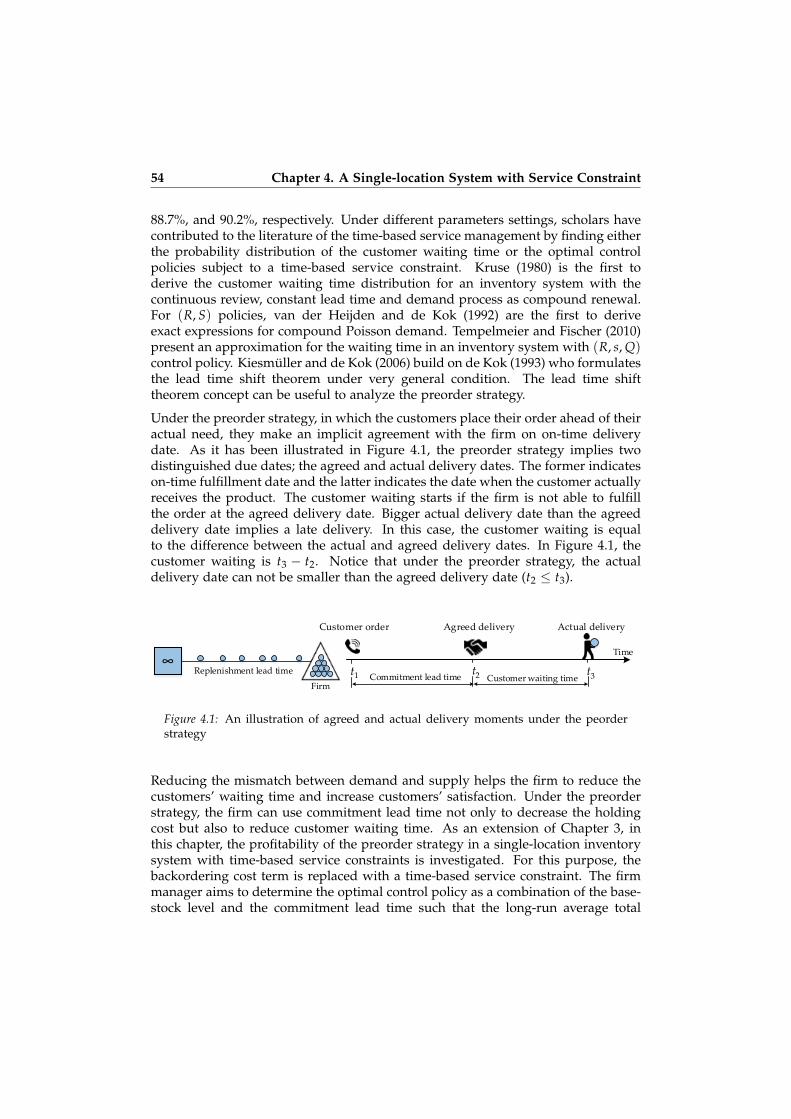
54 Chapter 4. A Single-location System with Service Constraint
88.7%, and 90.2%, respectively. Under different parameters settings, scholars havecontributed to the literature of the time-based service management by finding eitherthe probability distribution of the customer waiting time or the optimal controlpolicies subject to a time-based service constraint. Kruse (1980) is the first toderive the customer waiting time distribution for an inventory system with thecontinuous review, constant lead time and demand process as compound renewal.For (R, S) policies, van der Heijden and de Kok (1992) are the first to deriveexact expressions for compound Poisson demand. Tempelmeier and Fischer (2010)present an approximation for the waiting time in an inventory system with (R, s, Q)control policy. Kiesmuller and de Kok (2006) build on de Kok (1993) who formulatesthe lead time shift theorem under very general condition. The lead time shifttheorem concept can be useful to analyze the preorder strategy.
Under the preorder strategy, in which the customers place their order ahead of theiractual need, they make an implicit agreement with the firm on on-time deliverydate. As it has been illustrated in Figure 4.1, the preorder strategy implies twodistinguished due dates; the agreed and actual delivery dates. The former indicateson-time fulfillment date and the latter indicates the date when the customer actuallyreceives the product. The customer waiting starts if the firm is not able to fulfillthe order at the agreed delivery date. Bigger actual delivery date than the agreeddelivery date implies a late delivery. In this case, the customer waiting is equalto the difference between the actual and agreed delivery dates. In Figure 4.1, thecustomer waiting is t3 − t2. Notice that under the preorder strategy, the actualdelivery date can not be smaller than the agreed delivery date (t2 ≤ t3).
tt t
Agreed delivery Actual delivery
Commitment lead time Customer waiting time
Time
Replenishment lead time∞
Customer order
Firm321
Figure 4.1: An illustration of agreed and actual delivery moments under the peorderstrategy
Reducing the mismatch between demand and supply helps the firm to reduce thecustomers’ waiting time and increase customers’ satisfaction. Under the preorderstrategy, the firm can use commitment lead time not only to decrease the holdingcost but also to reduce customer waiting time. As an extension of Chapter 3, inthis chapter, the profitability of the preorder strategy in a single-location inventorysystem with time-based service constraints is investigated. For this purpose, thebackordering cost term is replaced with a time-based service constraint. The firmmanager aims to determine the optimal control policy as a combination of the base-stock level and the commitment lead time such that the long-run average total

4.1 Introduction 55
cost subject to a time-based service constraint is minimized. We distinguish twotime-based service measures as average customer waiting time and individual customerwaiting time. For the first measure, we define that the average customer waiting timeshould be less than or equal to a maximum waiting threshold ω, (ω ≥ 0). We referto the corresponding constraint optimization as Average Constraint Optimization(ACO) model. For the second, we define a time-based fill rate such that the fractionof the customers who experience a waiting time less than or equal to ω, is greaterthan or equal to a minimum service level η, (0 ≤ η ≤ 1). We formulate thistime-based measure as a chance constraint and refer to it as Chance ConstraintOptimization (CCO) model. Using the ACO and CCO models, we are going toanswer the following research questions:
1. When should the firm use preorder strategy?We find that the commitment lead time plays a significant role in thedetermination of the optimal control policy when either the maximum waitingthreshold is small enough (e.g., close to zero) or the minimum service levelis high enough (e.g., close to one). In other words, when the firm wants toprovide a quick response (i.e., ω → 0) to a high percentage of the customers(i.e., η → 1), the value of the commitment lead time in terms of cost reductionis more highlighted.
2. How can the optimal control policy be calculated?When the commitment lead time and a time-based service measure are takeninto account, the optimal commitment lead time is not always a bang-bangpolicy. Since for the above-mentioned settings, we are dealing with constraintoptimization problems, to the best of our knowledge, finding closed-formsolutions are very difficult and to some extent impossible. We develop exactand heuristic optimization algorithms for solving the ACO and CCO models.
3. What is the impact of the commitment lead time on the customer waiting time andoptimal cost value?We derive the exact probability distribution of the customer waiting timein terms of the system parameters and control policy. We show that thecommitment lead time not only increases the service level (i.e., the fraction ofthe customers who experience waiting up to a maximum waiting threshold),but also decreases the possible maximum waiting time that each customermight be faced. We find that for any arbitrary maximum waiting thresholdand minimum service level the optimal cost values of the both models arebounded above.
4. What is the impact of commitment lead time on the equivalent unit backordering costto maximum waiting threshold?We consider an unconstraint optimization model with backordering cost andits equivalent constraint optimization model with the average waiting timeconstraint. We find the equivalent unit backordering cost and maximum
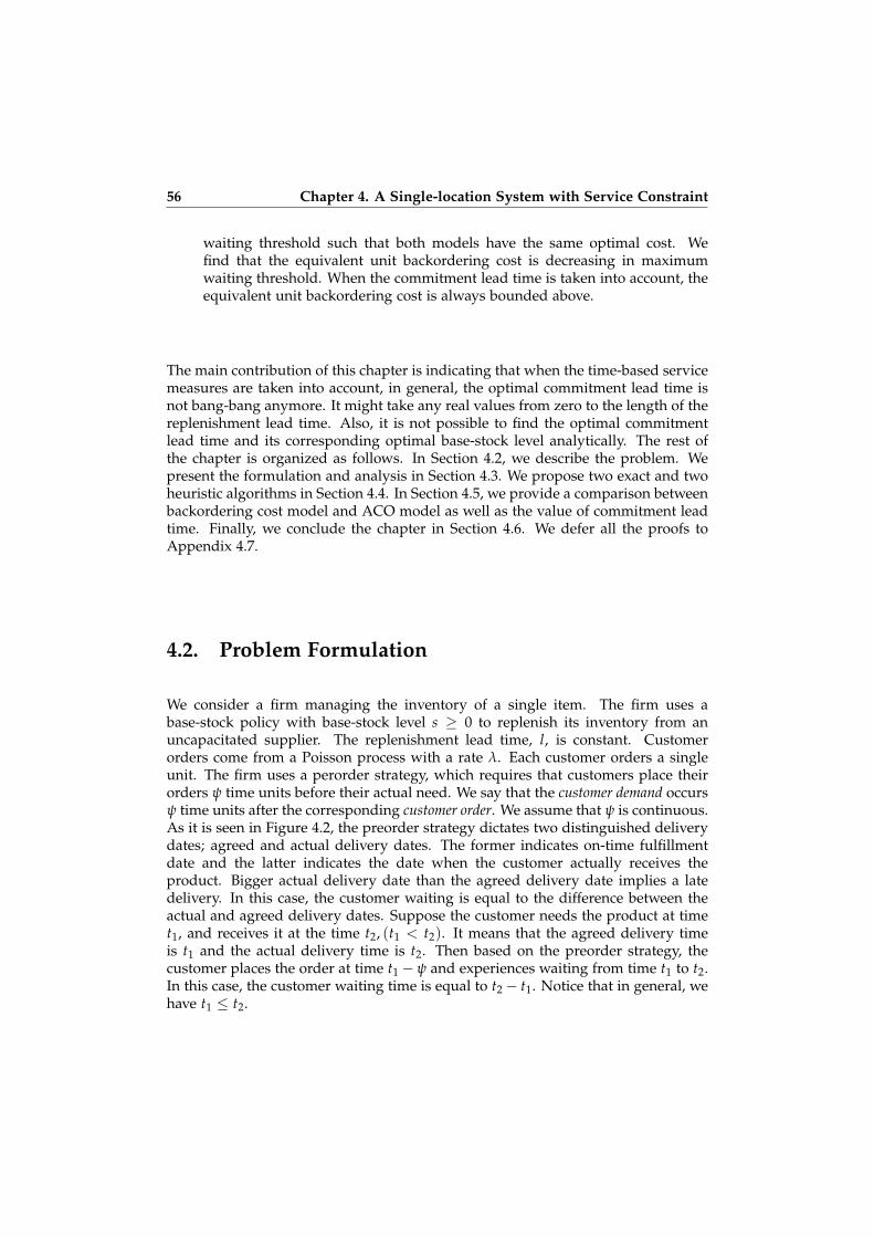
56 Chapter 4. A Single-location System with Service Constraint
waiting threshold such that both models have the same optimal cost. Wefind that the equivalent unit backordering cost is decreasing in maximumwaiting threshold. When the commitment lead time is taken into account, theequivalent unit backordering cost is always bounded above.
The main contribution of this chapter is indicating that when the time-based servicemeasures are taken into account, in general, the optimal commitment lead time isnot bang-bang anymore. It might take any real values from zero to the length of thereplenishment lead time. Also, it is not possible to find the optimal commitmentlead time and its corresponding optimal base-stock level analytically. The rest ofthe chapter is organized as follows. In Section 4.2, we describe the problem. Wepresent the formulation and analysis in Section 4.3. We propose two exact and twoheuristic algorithms in Section 4.4. In Section 4.5, we provide a comparison betweenbackordering cost model and ACO model as well as the value of commitment leadtime. Finally, we conclude the chapter in Section 4.6. We defer all the proofs toAppendix 4.7.
4.2. Problem Formulation
We consider a firm managing the inventory of a single item. The firm uses abase-stock policy with base-stock level s ≥ 0 to replenish its inventory from anuncapacitated supplier. The replenishment lead time, l, is constant. Customerorders come from a Poisson process with a rate λ. Each customer orders a singleunit. The firm uses a perorder strategy, which requires that customers place theirorders ψ time units before their actual need. We say that the customer demand occursψ time units after the corresponding customer order. We assume that ψ is continuous.As it is seen in Figure 4.2, the preorder strategy dictates two distinguished deliverydates; agreed and actual delivery dates. The former indicates on-time fulfillmentdate and the latter indicates the date when the customer actually receives theproduct. Bigger actual delivery date than the agreed delivery date implies a latedelivery. In this case, the customer waiting is equal to the difference between theactual and agreed delivery dates. Suppose the customer needs the product at timet1, and receives it at the time t2, (t1 < t2). It means that the agreed delivery timeis t1 and the actual delivery time is t2. Then based on the preorder strategy, thecustomer places the order at time t1 − ψ and experiences waiting from time t1 to t2.In this case, the customer waiting time is equal to t2− t1. Notice that in general, wehave t1 ≤ t2.
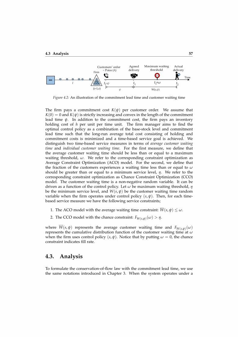
4.3 Analysis 57
tt -ψ t
~ Poiss (λ)
Agreed delivery
Actual delivery
ω
ψ W(s,ψ)
Time
(s-1,s)
l∞
Customers’ order Maximum waiting threshold
t +ω
Firm
11 1 2
Figure 4.2: An illustration of the commitment lead time and customer waiting time
The firm pays a commitment cost K(ψ) per customer order. We assume thatK(0) = 0 and K(ψ) is strictly increasing and convex in the length of the commitmentlead time ψ. In addition to the commitment cost, the firm pays an inventoryholding cost of h per unit per time unit. The firm manager aims to find theoptimal control policy as a combination of the base-stock level and commitmentlead time such that the long-run average total cost consisting of holding andcommitment costs is minimized and a time-based service goal is achieved. Wedistinguish two time-based service measures in terms of average customer waitingtime and individual customer waiting time. For the first measure, we define thatthe average customer waiting time should be less than or equal to a maximumwaiting threshold, ω. We refer to the corresponding constraint optimization asAverage Constraint Optimization (ACO) model. For the second, we define thatthe fraction of the customers experiences a waiting time less than or equal to ωshould be greater than or equal to a minimum service level, η. We refer to thecorresponding constraint optimization as Chance Constraint Optimization (CCO)model. The customer waiting time is a non-negative random variable. It can bedriven as a function of the control policy. Let ω be maximum waiting threshold, ηbe the minimum service level, and W(s, ψ) be the customer waiting time randomvariable when the firm operates under control policy (s, ψ). Then, for each time-based service measure we have the following service constraints;
1. The ACO model with the average waiting time constraint: W(s, ψ) ≤ ω.
2. The CCO model with the chance constraint: FW(s,ψ)(ω) > η.
where W(s, ψ) represents the average customer waiting time and FW(s,ψ)(ω)represents the cumulative distribution function of the customer waiting time at ωwhen the firm uses control policy (s, ψ). Notice that by putting ω = 0, the chanceconstraint indicates fill rate.
4.3. Analysis
To formulate the conservation-of-flow law with the commitment lead time, we usethe same notations introduced in Chapter 3. When the system operates under a
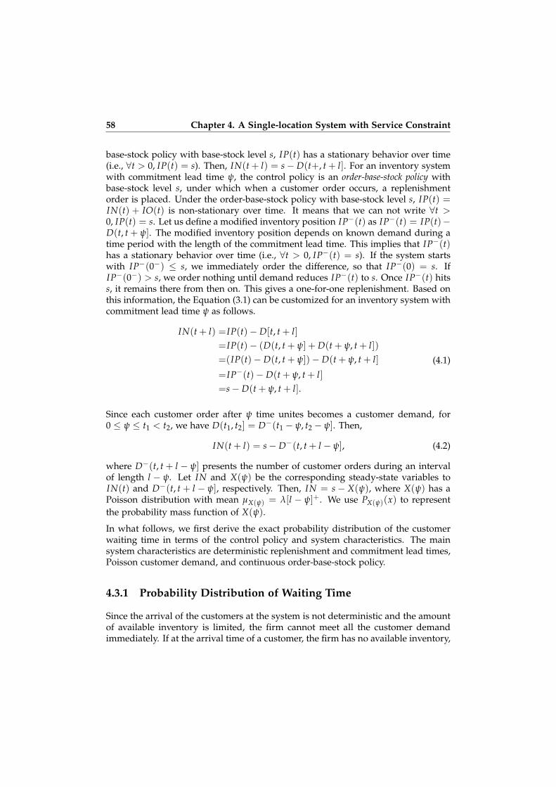
58 Chapter 4. A Single-location System with Service Constraint
base-stock policy with base-stock level s, IP(t) has a stationary behavior over time(i.e., ∀t > 0, IP(t) = s). Then, IN(t + l) = s− D(t+, t + l]. For an inventory systemwith commitment lead time ψ, the control policy is an order-base-stock policy withbase-stock level s, under which when a customer order occurs, a replenishmentorder is placed. Under the order-base-stock policy with base-stock level s, IP(t) =IN(t) + IO(t) is non-stationary over time. It means that we can not write ∀t >0, IP(t) = s. Let us define a modified inventory position IP−(t) as IP−(t) = IP(t)−D(t, t + ψ]. The modified inventory position depends on known demand during atime period with the length of the commitment lead time. This implies that IP−(t)has a stationary behavior over time (i.e., ∀t > 0, IP−(t) = s). If the system startswith IP−(0−) ≤ s, we immediately order the difference, so that IP−(0) = s. IfIP−(0−) > s, we order nothing until demand reduces IP−(t) to s. Once IP−(t) hitss, it remains there from then on. This gives a one-for-one replenishment. Based onthis information, the Equation (3.1) can be customized for an inventory system withcommitment lead time ψ as follows.
IN(t + l) =IP(t)− D[t, t + l]=IP(t)− (D(t, t + ψ] + D(t + ψ, t + l])=(IP(t)− D(t, t + ψ])− D(t + ψ, t + l]
=IP−(t)− D(t + ψ, t + l]=s− D(t + ψ, t + l].
(4.1)
Since each customer order after ψ time unites becomes a customer demand, for0 ≤ ψ ≤ t1 < t2, we have D(t1, t2] = D−(t1 − ψ, t2 − ψ]. Then,
IN(t + l) = s− D−(t, t + l − ψ], (4.2)
where D−(t, t + l − ψ] presents the number of customer orders during an intervalof length l − ψ. Let IN and X(ψ) be the corresponding steady-state variables toIN(t) and D−(t, t + l − ψ], respectively. Then, IN = s− X(ψ), where X(ψ) has aPoisson distribution with mean µX(ψ) = λ[l − ψ]+. We use PX(ψ)(x) to representthe probability mass function of X(ψ).
In what follows, we first derive the exact probability distribution of the customerwaiting time in terms of the control policy and system characteristics. The mainsystem characteristics are deterministic replenishment and commitment lead times,Poisson customer demand, and continuous order-base-stock policy.
4.3.1 Probability Distribution of Waiting Time
Since the arrival of the customers at the system is not deterministic and the amountof available inventory is limited, the firm cannot meet all the customer demandimmediately. If at the arrival time of a customer, the firm has no available inventory,

4.3 Analysis 59
the firm is not able to provide an immediate delivery to the corresponding customer.Consequently, the customer has to wait until the replenishment order, which canbe used to satisfy the demand, arrives at the system. The waiting time of eachcustomer depends on the status of the system at the customer’s arrival time. Sincethe status of the system is changing over time, the waiting time of the customer isa random variable. In general, the customer waiting time depends on the systemcharacteristics such as demand rate, replenishment lead time, and control policy(i.e., base-stock level and commitment lead time). Since the firm operates under thepreorder strategy, it receives ADI from the customers and it can use this informationto make more cost-efficient decisions while reducing the customer waiting time.
Notice that if ψ > l, the firm can provide on-time delivery without holdinginventory by placing a replenishment order ψ− l time units after a customer orderoccurs. This results in zero holding and zero customer waiting time. In thischapter, we analyze the case with 0 ≤ ψ ≤ l. It is obvious that in a stock-outsituation, the length of the customer waiting time varies from 0 to l − ψ. Hence,W(s, ψ) ∈ [0, l − ψ]. For W(s, ψ), we derive the probability mass at zero PW(s,ψ)(0),the probability density function fW(s,ψ)(τ) and cumulative distribution functionFW(s,ψ)(τ) in Theorem 4.1.
Theorem 4.1 In a single-location inventory system, for given s ∈N0, and ψ ∈ [0, l],
1. the probability mass of the customer waiting time at zero is given by
PW(s,ψ)(0) =s−1
∑k=0
µkX(ψ)
k!e−µX(ψ) ,
2. the probability density function of the customer waiting time is
fW(s,ψ)(τ) =
λ(µX(ψ)−λτ)
s−1
(s−1)! e−(µX(ψ)−λτ) 0 < τ < l − ψ,
0 τ ≥ l − ψ,
3. the cumulative distribution function of the customer waiting time is
FW(s,ψ)(τ) =
s−1∑
k=0
(µX(ψ)−λτ)k
k! e−(µX(ψ)−λτ) 0 ≤ τ < l − ψ,
1 τ ≥ l − ψ,
where µX(ψ) = λ(l − ψ).
We refer to Appendix 4.7.1 for the proof. As it is seen from Theorem 4.1, thecommitment lead time decreases the possible maximum waiting time from l to l−ψ
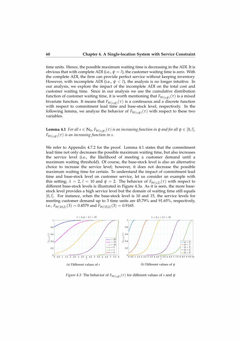
60 Chapter 4. A Single-location System with Service Constraint
time units. Hence, the possible maximum waiting time is decreasing in the ADI. It isobvious that with complete ADI (i.e., ψ = l), the customer waiting time is zero. Withthe complete ADI, the firm can provide perfect service without keeping inventory.However, with incomplete ADI (i.e., ψ < l), the analysis is no longer intuitive. Inour analysis, we explore the impact of the incomplete ADI on the total cost andcustomer waiting time. Since in our analysis we use the cumulative distributionfunction of customer waiting time, it is worth mentioning that FW(s,ψ)(τ) is a mixedbivariate function. It means that FW(s,ψ)(τ) is a continuous and a discrete functionwith respect to commitment lead time and base-stock level, respectively. In thefollowing lemma, we analyze the behavior of FW(s,ψ)(τ) with respect to these twovariables.
Lemma 4.1 For all s ∈N0, FW(s,ψ)(τ) is an increasing function in ψ and for all ψ ∈ [0, l],FW(s,ψ)(τ) is an increasing function in s.
We refer to Appendix 4.7.2 for the proof. Lemma 4.1 states that the commitmentlead time not only decreases the possible maximum waiting time, but also increasesthe service level (i.e., the likelihood of meeting a customer demand until amaximum waiting threshold). Of course, the base-stock level is also an alternativechoice to increase the service level; however, it does not decrease the possiblemaximum waiting time for certain. To understand the impact of commitment leadtime and base-stock level on customer service, let us consider an example withthis setting; λ = 2, l = 10 and ψ = 2. The behavior of FW(s,2)(τ) with respect todifferent base-stock levels is illustrated in Figure 4.3a. As it is seen, the more base-stock level provides a high service level but the domain of waiting time still equals[0, l]. For instance, when the base-stock level is 10 and 15, the service levels formeeting customer demand up to 3 time units are 45.79% and 91.65%, respectively,i.e., FW(10,2)(3) = 0.4579 and FW(15,2)(3) = 0.9165.
0 0.5 1 1.5 2 2.5 3 3.5 4 4.5 5 5.5 6 6.5 7 7.5 80
0.2
0.4
0.6
0.8
1
τ
F W(s
,2)(
τ)
λ = 2, ψ = 2, l = 10
s = 20s = 15s = 10s = 5s = 1s = 0
(a) Different values of s
0 0.5 1 1.5 2 2.5 3 3.5 4 4.5 5 5.5 6 6.5 7 7.5 8 8.5 9 9.5 100
0.2
0.4
0.6
0.8
1
τ
F W(3
,ψ)(
τ)
λ = 2, s = 3, l = 10
ψ = 9ψ = 7ψ = 5ψ = 2ψ = 0
(b) Different values of ψ
Figure 4.3: The behavior of FW(s,ψ)(τ) for different values of s and ψ

4.3 Analysis 61
Furthermore, for a given base-stock level s = 3 and different values of thecommitment lead time ψ, the service levels are illustrated in Figure 4.3b. Forexample, when the firm uses preorder strategies with ψ = 5 and ψ = 10 (completeADI), the service levels for meeting customer demand up to 3 time units are 23.81%and 100%, respectively, i.e., FW(3,5)(3) = 0.2381 and FW(3,10)(3) = 1.
4.3.2 Cost Function
In this section, we derive an expression for the long-run average total cost function.The cost function is comprised of inventory holding and commitment costs. FromChapter 3, remember that IN = s− X(ψ), where X(ψ) is the cumulative demandduring l − ψ. Then, X(ψ) also has a Poisson distribution with mean µX(ψ) = λ(l −ψ). Define C(s, ψ) as the long-run average total cost when a base-stock level s isused and a commitment lead time ψ is provided. Similar to Chapter 3, C(s, ψ) canbe written as follows;
C(s, ψ) =hE {max(0, IN)}+ λK(ψ)
=h(
sFX(ψ)(s)− µX(ψ)FX(ψ)(s− 1))+ λK(ψ),
(4.3)
where FX(ψ)(x) is the cumulative distribution function of X(ψ). It is worthemphasizing that our analysis and results hold for any form of K(ψ) as long asit is increasing and convex in ψ and K(0) = 0. In the rest of this chapter, for easeof exposition, we restrict our analysis to a linear unit commitment cost c per timeunit. Therefore, for all s ∈ N0 and ψ ∈ [0, l], the cost function can be rewritten asfollows;
C(s, ψ) = h(
sFX(ψ)(s)− µX(ψ)FX(ψ)(s− 1))+ cλψ. (4.4)
C(s, ψ) is a discrete function with respect to s and a continuous function withrespect to ψ. Based on Lemmas 3.1 and 3.2 in Chapter 3, we know that for alls ∈ N, C(s, ψ) is strictly increasing and convex in ψ and for all ψ ∈ [0, l], C(s, ψ)is increasing and convex in s. For a given commitment lead time ψ, increasing thebase-stock level s results in increasing average holding cost (intuitive). For a givenbase-stock level s, increasing ψ results in an increase not only in the commitmentcost, but also in the holding cost (counter-intuitive). Logically, with more ADI, areduction in the average holding cost is expected. However, since the base-stockis fixed, by increasing ψ, the firm actually keeps more inventory than the requiredamount while the firm needs less inventory since ADI is available.

62 Chapter 4. A Single-location System with Service Constraint
4.3.3 Constraints on the Customer Waiting Time
In this section, the ACO and CCO models are analyzed. We use subscripts a and cto refer to the ACO and CCO models, respectively.
4.3.3.1 The ACO Model
The commitment lead time is an agreement between the customers and the firm.The customer waiting time starts after the duration of commitment lead time. Asit is shown in Figure 4.2, the customer order lead time is the summation of thecommitment lead time and the customer waiting time. Since the commitment leadtime is deterministic, the customer waiting time W(s, ψ) is a proper representativeof the customer order lead time. Using Theorem 4.1, we derive the average customerwaiting time in Proposition 4.1.
Proposition 4.1 In a single-location inventory system, for all s ∈ N0 and ψ ∈ [0, l], theaverage customer waiting time W(s, ψ) is given by
W(s, ψ) =1λ
(sFX(ψ)(s)− µX(ψ)FX(ψ)(s− 1) + µX(ψ) − s
).
See Appendix 4.7.3 for the proof. According to Proposition 4.1, W(s, ψ) is nonlinearin the base-stock level s and the commitment lead time ψ. W(s, ψ) is a discretefunction in s and a continuous function in ψ. The following Lemma is useful tounderstand the behavior of W(s, ψ) with respect to s and ψ.
Lemma 4.2 In a single-location inventory system,
1. for all s ∈N0, the average customer waiting time W(s, ψ) is non-increasing in ψ.
2. for all ψ ∈ [0, l], the average customer waiting time W(s, ψ) is non-increasing in s.
We defer the proofs to Appendices 4.7.4 and 4.7.8. According to Lemma 4.2, theaverage waiting time can be reduced by increasing the base-stock level s and/orincreasing the commitment lead time ψ. The decision on which one of these twois more beneficial and cost efficient depends on the cost parameters and amount ofreduction in the average waiting time. For the aforementioned parameter stettingin Subsection 4.3.1, we plot W(s, ψ) with respect to commitment lead time ψ fordifferent base-stock levels. As seen in Figure 4.4, when s = 0, there is a linearnegative correlation between W(s, ψ) and ψ (i.e., W(s, ψ) = l − ψ). For positivebase-stock levels, this negative correlation is not linear anymore. For all s ∈N0, thereduction in average waiting time is non-increasing in ψ.

4.3 Analysis 63
0 0.5 1 1.5 2 2.5 3 3.5 4 4.5 5 5.5 6 6.5 7 7.5 8 8.5 9 9.5 100123456789
10
Commitment lead time (ψ)
W(s
,ψ)
s = 0s = 2s = 4s = 8s = 16
Figure 4.4: The behavior of W(s, ψ) with respect to commitment lead time ψ
Using Proposition 4.1 and Equation (4.4), we can formulate the ACO model asfollows;
(ACO) : mins,ψ
C(s, ψ) = h(
sFX(ψ)(s)− µX(ψ)FX(ψ)(s− 1))+ cλψ,
subject to: φa(s, ψ) ≤ 0,s ∈N0, ψ ∈ [0, l],
(4.5)
where φa(s, ψ) = sFX(ψ)(s) − µX(ψ)FX(ψ)(s − 1) + µX(ψ) − s − λω. Since the ACOmodel is a Constraint Mixed-integer Nonlinear Program (C-MINLP), to the bestof our knowledge, finding a closed-form solution to this problem is impossible.To overcome this difficulty, we analyze φa(s, ψ) to determine the feasible region ofthe optimization problem (4.5). The results of our analysis are presented in thefollowing Lemma.
Lemma 4.3 For all s ∈N0, φa(s, ψ) is non-increasing in ψ, and for all ψ ∈ [0, l], φa(s, ψ)is non-increasing in s.
See Appendix 4.7.6 for the proof. For all ψ ∈ [0, l], minimizing C(s, ψ) over s ∈ N0provides one-to-one relationship between s and ψ. Let us define sψ as the optimalbase-stock level for a given ψ. Then, we can obtain a tight lower bound Ca(sψ, ψ)on [0, l] as follows;
Ca(sψ, ψ) = mins∈N0
C(s, ψ) s.t. φa(s, ψ) ≤ 0. (4.6)
By solving optimization (4.6), the interval [0, l] as domain of univariate functionCa(sψ, ψ), is divided into s0
a + 1 subintervals such that
[0, l] = [ψs0a, ψs0
a−1] ∪ [ψs0a−1, ψs0
a−2] ∪ ...∪ [ψ2, ψ1] ∪ [ψ0, l],
where 0 = ψs0a< ψs0
a−1 < ... < ψ1 < ψ0 and s0a = {s ∈ N0 : φa(s, 0) ≤ 0 < φa(s−
1, 0)}. Since for all s = 0, 1, 2, ..., s0a − 1 the subinterval formed by beakpoints ψs+1

64 Chapter 4. A Single-location System with Service Constraint
and ψs corresponds to base-stock s, we refer to it as Ψs = [ψs+1, ψs]. In other words,Ca(sψ, ψ) is a discontinuous piecewise-convex function with step sizes Ψs. Actually, Ψsrefers to a subinterval on [0, l] such that for all ψ ∈ Ψs, we have Ca(sψ, ψ) = C(s, ψ)(see Figure 4.5). Let Θa be the set of all the breakpoints ψs of the ACO model.
Then, Θa =⋃s0
as=0 {ψs}, where |Θa| = s0
a + 1. Notice that for all ψs ∈ Θa\{0}, wehave φa(s, ψs) = 0. Hence, solving φa(0, ψ0) = 0 yields ψ0 = l − ω. Then, ψs0
a= 0
and ψ0 = l − ω are the smallest and largest elements of the breakpoint set Θa,respectively.
0 1 2 3 4 5 6 7 8 9 1035
40
45
50
55
60
65
70
75
C(0, ψ)
C(1, ψ)
C(2, ψ)C(3, ψ)C(4, ψ)C(5, ψ)
C(6, ψ)C(7, ψ)
infeasible region
feasible region
Ψ7 Ψ6 Ψ5 Ψ4 Ψ3 Ψ2 Ψ1 Ψ0
Commitment lead time (ψ)
Ca(
sψ,ψ
)
λ = 0.5, h = 20, c = 10, ω = 0.6, l = 10
Figure 4.5: The discontinuous piecewise nonlinear function Ca(sψ, ψ) on [0, l]
Based on the properties of φa(s, ψ), we know that the smallest value of s correspondsto the largest value of ψ (i.e., ψs0
a< ψs0
a−1 < ... < ψ1 < ψ0). Since the cost function isincreasing in s and ψ, the smallest pair of (s, ψ) provides the minimum value of thecost. Because the optimal values of s and ψ are dependent on each other, findingthe the best s and ψ that guarantees an optimal trade-off between the holding andcommitment costs is not a straightforward task.
Different values of the maximum waiting threshold ω provide different feasibleregions. It means that maximum waiting threshold ω can change the optimalcontrol policy. To illustrate the impact of ω on the behavior of Ca(sψ, ψ) andoptimal control policy, consider two settings with different values of ω and commonparameters as; λ = 3, h = 15, c = 2.2, and l = 10. As it is shown in Figure 4.6, whenthe waiting time threshold ω is changed from 0.35 to 0.10, the optimal controlpolicy is changed from (32, 0.28) to (0, 9.90). In the setting with ω = 0.1, the role ofcommitment lead time in the optimal control policy is more highlighted.

4.3 Analysis 65
0 1 2 3 4 5 6 7 8 9 1060
62
64
66
68
70
72
74
76
78
Commitment lead time (ψ)
Ca(
sψ,ψ
)
ω = 0.35, s∗ = 32, ψ∗ = 0.28, C(s∗, ψ) = 60.24
0 1 2 3 4 5 6 7 8 9 1060
70
80
90
100
110
120
130
Commitment lead time (ψ)
Ca(
sψ,ψ
)
ω = 0.1, s∗ = 0, ψ∗ = 9.9, C(s∗, ψ) = 65.34
Figure 4.6: Behavior of Ca(sψ, ψ) in terms of ψ for different values of ω
As shown in Figure 4.6, the optimal control policy and the corresponding averagecost depend on ω. The following proposition states the overall behavior of optimalcost in terms of ω.
Proposition 4.2 In the ACO model, for all ψ ∈ [0, l], ω ∈ [0, l], and s ∈ N0, the optimalcost Ca(s∗, ψ∗),
1. is non-increasing in the maximum waiting threshold ω.
2. is bounded above by cµX(ω).
We refer to Appendices 4.7.7 and 4.7.8 for the proofs. According to Proposition 4.2.1,when the firm targets a bigger maximum waiting threshold on the average waitingtime, it needs less inventory or shorter commitment lead time. Consequently, itresults in less holding and commitment costs. Furthermore, Proposition 4.2.2 statesthat the optimal cost subject to any value of the maximum waiting threshold isbounded. In other words, for any value of the maximum waiting threshold, thereis a trade-off between commitment and holding costs. More specifically, when thefirm targets a very quick response (i.e., ω close to zero), the firm should enticethe customers to provide complete ADI (i.e., ψ = l − ω). In this situation, thecommitment cost is the only cost which is charged and equal to cµX(ω).
4.3.3.2 The CCO Model
Instead of looking at the average waiting time as a time-based service measure in theACO model, we now look at individual customer waiting time. For this purpose,we introduce a time-based service measure in the form of a chance constraint.In other words, we would like to find the optimal control policy such that adesired percentage (i.e., η) of the customers receive service within a time frame

66 Chapter 4. A Single-location System with Service Constraint
(i.e., maximum waiting threshold ω). For instance, we aim to meet 95% of thecustomers demand within 4 hours. This type of service measure is recommendedwhen customer waiting time variability is high. We refer to the optimization modelwith this type of service measure as chance constraint optimization (CCO) model.For given ω ∈ [0, l], η ∈ [0, 1] and using Theorem 4.1, the chance constraint can bewritten in terms of the cumulative distribution function of Poisson distribution asfollows.
P(W(s, ψ) ≤ ω) = FW(s,ψ)(ω) =s−1
∑k=0
(µX(ψ) −ωλ
)k
k!e−(µX(ψ)−ωλ). (4.7)
As seen in Equation (4.7), FW(s,ψ)(ω) can be rewritten as the cumulative distributionfunction of the Poisson random variable Y(ω, ψ) at s − 1 with mean µY(ω,ψ) =
µX(ψ) − ωλ. Hence, FW(s,ψ)(ω) = FY(ω,ψ)(s− 1). Therefore, the CCO model can beformulated as follows:
(CCO) : mins,ψ
C(s, ψ) = h(
sFX(ψ)(s)− µX(ψ)FX(ψ)(s− 1))+ cλ
subject to: φc(s, ψ) ≤ 0s ∈N0, ψ ∈ [0, l],
(4.8)
where φc(s, ψ) = η − FY(ω,ψ)(s− 1). Recall that FX(ψ)(s) and FY(ω,ψ)(s− 1) are thecumulative distribution function of the Poisson distribution with mean µX(ψ) =
λ(l − ψ) and µY(ω,ψ) = µX(ψ) − ωλ, respectively. Similar to the ACO model, theCCO model is also C-MINLP and finding a closed-form solution to this problem isdifficult and to some extent impossible. To find the optimal solution, we analyzeφc(s, ψ) and determine the feasible region of 4.8. The results of our analysis arepresented in the following Lemma.
Lemma 4.4 For all s ∈N0, φc(s, ψ) is non-increasing in ψ and for all ψ ∈ [0, l], φc(s, ψ)is non-increasing in s.
See Appendix 4.7.13 for the proof. Following the same approach as the ACO model,we can get a tight lower bound Cc(sψ, ψ) by solving
Cc(sψ, ψ) = mins∈N0
C(s, ψ), s.t. φc(s, ψ). (4.9)
By solving optimization (4.9), the interval [0, l] as domain of univariate functionCc(sψ, ψ), is divided into s0
c subintervals such that
[0, l] = [ψs0c, ψs0
c−1] ∪ [ψs0c−1, ψs0
c−2] ∪ ...∪ [ψ2, ψ1] ∪ [ψ1, l],
where 0 = ψs0c< ψs0
c−1 < ... < ψ1 and s0c = {s ∈ N0 : φc(s, 0) ≤ 0 < φc(s− 1, 0)}.
Since for all s = 1, 2, ..., s0c − 1 the subinterval formed by beakpoints ψs+1 and ψs
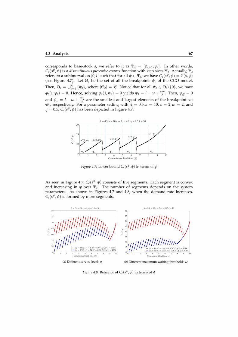
4.3 Analysis 67
corresponds to base-stock s, we refer to it as Ψs = [ψs+1, ψs]. In other words,Cc(sψ, ψ) is a discontinuous piecewise-convex function with step sizes Ψs. Actually, Ψsrefers to a subinterval on [0, l] such that for all ψ ∈ Ψs, we have Cc(sψ, ψ) = C(s, ψ)(see Figure 4.7). Let Θc be the set of all the breakpoints ψs of the CCO model.
Then, Θc =⋃s0
cs=1 {ψs}, where |Θc| = s0
c . Notice that for all ψs ∈ Θc\{0}, we haveφc(s, ψs) = 0. Hence, solving φc(1, ψ1) = 0 yields ψ1 = l − ω + lnη
λ . Then, ψs0c= 0
and ψ1 = l − ω + lnηλ are the smallest and largest elements of the breakpoint set
Θc, respectively. For a parameter setting with λ = 0.5, h = 10, c = 2, ω = 2, andη = 0.5, Cc(sψ, ψ) has been depicted in Figure 4.7.
0 1 2 3 4 5 6 7 8 9 105
10
15
20
C(1, ψ)C(2, ψ)
C(3, ψ)C(4, ψ)C(5, ψ)
Ψ1Ψ2Ψ3Ψ4Ψ5
Commitment lead time (ψ)
Cc(
sψ,ψ
)
λ = 0.5, h = 10, c = 2, ω = 2, η = 0.5, l = 10
Figure 4.7: Lower bound Cc(sψ, ψ) in terms of ψ
As seen in Figure 4.7, Cc(sψ, ψ) consists of five segments. Each segment is convexand increasing in ψ over Ψs. The number of segments depends on the systemparameters. As shown in Figures 4.7 and 4.8, when the demand rate increases,Cc(sψ, ψ) is formed by more segments.
0 1 2 3 4 5 6 7 8 9 1045
50
55
60
65
70
75
80
(η = 0.95) : s∗ = 1, ψ∗ = 8.97, C(s∗, ψ∗) = 55.14(η = 0.90) : s∗ = 24, ψ∗ = 0.01, C(s∗, ψ∗) = 45.16
Commitment lead time (ψ)
Cc(
sψ,ψ
)
λ = 2, h = 10, c = 3, ω = 1, l = 10
(a) Different service levels η
0 1 2 3 4 5 6 7 8 9 1040
45
50
55
60
65
70
75
80
(ω = 1) : s∗ = 1, ψ∗ = 8.97, C(s∗, ψ∗) = 55.14(ω = 2) : s∗ = 23, ψ∗ = 0.14, C(s∗, ψ∗) = 39.91
Commitment lead time (ψ)
Cc(
sψ,ψ
)
λ = 2, h = 10, c = 3, η = 0.95, l = 10
(b) Different maximum waiting thresholds ω
Figure 4.8: Behavior of Cc(sψ, ψ) in terms of ψ

68 Chapter 4. A Single-location System with Service Constraint
When service level η is significantly high compared to the base-stock level,commitment lead time plays a stronger role in forming the optimal control policy.In Figure 4.8a, by changing η from 0.90 to 0.95, the optimal commitment lead timeis changed from 0.01 to 8.97. Moreover, when maximum waiting threshold ω issignificantly small, commitment lead time plays a stronger role in optimal controlpolicy. For instance, in Figure 4.8b, decreasing the value of ω from 2 to 1 results inan increase in the optimal commitment lead time from 0.14 to 8.97.
As shown in Figure 4.8, the optimal control policy and the corresponding averagecost depend on both η and ω. The following proposition states the overall behaviorof optimal cost in terms of η and ω and other system parameters.
Proposition 4.3 In the CCO model, for all ψ ∈ [0, l], ω ∈ [0, l], η ∈ [0, 1], and s ∈ N0,the optimal cost Cc(s∗, ψ∗), is bounded above by h
η e−µX(ω) + c(
lnη + µX(ω)
).
We refer to Appendix 4.7.9 for the proof. Proposition 4.3 states that the optimalcost subject to any value of the maximum waiting threshold ω and service level ηis bounded. In other words, for any value of the maximum waiting threshold, thereis a trade-off between commitment and holding costs. More specifically, when thefirm targets a very quick response (i.e., ω close to zero) or high service level (i.e.,η close to one), the firm should entice the customers to provide complete ADI (i.e.,ψ = l − ω + lnη
λ ). In this situation, the commitment cost is the only cost which is
charged and equal to hη e−µX(ω) + c
(lnη + µX(ω)
).
4.3.3.3 Immediate Fill Rate
Under the preorder strategy, the immediate fill rate refers to the fraction of thecustomers who receive an on-time fulfillment. In other words, the fraction of thecustomers who receives the product at the moment of the need. By setting ω = 0 inthe chance constraint, the immediate fill rate can be defined as FW(s,ψ)(0) ≥ η. Sincecustomer demand comes from a pure Poisson process and fulfillment of demandis based on a First-Come, First-Served (FCFS) allocation rule, as an equivalence ofzero waiting time, we can write P(W(s, ψ) = 0) = P(IN > 0). Using this definition,we conjecture the following result on the optimal commitment lead time.
Conjecture 4.1 The optimal commitment lead time and its corresponding base-stock level of the single location inventory system with immediate fill raterequirement happens either at ψs0
cor ψ1.
Based on Conjecture 4.1, the optimal commitment lead time happens either at 0 orl + lnη
λ . In other words, by changing the support of commitment lead time from
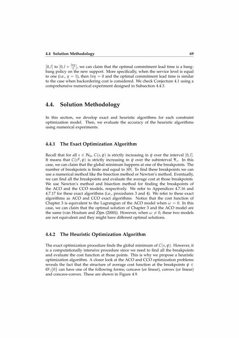
4.4 Solution Methodology 69
[0, l] to [0, l + lnηλ ], we can claim that the optimal commitment lead time is a bang-
bang policy on the new support. More specifically, when the service level is equalto one (i.e., η = 1), then lnη = 0 and the optimal commitment lead time is similarto the case when backordering cost is considered. We check Conjecture 4.1 using acomprehensive numerical experiment designed in Subsection 4.4.3.
4.4. Solution Methodology
In this section, we develop exact and heuristic algorithms for each constraintoptimization model. Then, we evaluate the accuracy of the heuristic algorithmsusing numerical experiments.
4.4.1 The Exact Optimization Algorithm
Recall that for all s ∈ N0, C(s, ψ) is strictly increasing in ψ over the interval [0, l].It means that C(sψ, ψ) is strictly increasing in ψ over the subinterval Ψs. In thiscase, we can claim that the global minimum happens at one of the breakpoints. Thenumber of breakpoints is finite and equal to |Θ|. To find these breakpoints we canuse a numerical method like the bisection method or Newton’s method. Eventually,we can find all the breakpoints and evaluate the average cost at those breakpoints.We use Newton’s method and bisection method for finding the breakpoints ofthe ACO and the CCO models, respectively. We refer to Appendices 4.7.16 and4.7.17 for these exact algorithms (i.e., procedures 3 and 4). We refer to these exactalgorithms as ACO and CCO exact algorithms. Notice that the cost function ofChapter 3 is equivalent to the Lagrangian of the ACO model when ω = 0. In thiscase, we can claim that the optimal solution of Chapter 3 and the ACO model arethe same (van Houtum and Zijm (2000)). However, when ω 6= 0, these two modelsare not equivalent and they might have different optimal solutions.
4.4.2 The Heuristic Optimization Algorithm
The exact optimization procedure finds the global minimum of C(s, ψ). However, itis a computationally intensive procedure since we need to find all the breakpointsand evaluate the cost function at those points. This is why we propose a heuristicoptimization algorithm. A closer look at the ACO and CCO optimization problemsreveals the fact that the structure of average cost function at the breakpoints ψ ∈Θ\{0} can have one of the following forms; concave (or linear), convex (or linear)and concave-convex. These are shown in Figure 4.9.
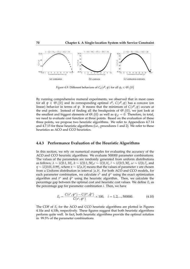
70 Chapter 4. A Single-location System with Service Constraint
0.14 1 2 3 4 5 6 7 8 9 9.764.02
66
68
70.18
Commitment lead time (ψ)
Ca(
sψ,ψ
)
λ = 3, h = 15, c = 2.2, ω = 0.3, l = 10
(a) concave
0 1 2 3 4 5 6 7 8 9.146.37
48
50
52
54
5657.33
Commitment lead time (ψ)
Ca(
sψ,ψ
)
λ = 9, h = 40, c = 0.7, ω = 0.9, l = 10
(b) convex
0.1 2 4 6 8 10 12 14 16 19.587.14
88
89
90
91
9292.66
Commitment lead time (ψ)
Ca(
sψ,ψ
)
λ = 5, h = 15, c = 0.9, ω = 0.5, l = 20
(c) concave-convex
Figure 4.9: Different behaviors of Ca(sψ, ψ) for all ψs ∈ Θ\{0}
By running comprehensive numeral experiments, we observed that in most casesfor all ψ ∈ Θ\{0} and its corresponding optimal sψ, C(sψ, ψ) has a concave (onlinear) behavior in terms of ψ. It means that the minimum of C(sψ, ψ) occurs atthe end points. Instead of finding all the breakpoints of Θ\{0}, we just look atthe smallest and biggest elements of Θ\{0} as well as ψs0 = 0. Therefore, in total,we need to evaluate cost function at three points. Based on the evaluation of thesethree points, we propose two heuristic algorithms. We refer to Appendices 4.7.14and 4.7.15 for these heuristic algorithms (i.e., procedures 1 and 2). We refer to theseheuristics as ACO and CCO heuristics.
4.4.3 Performance Evaluation of the Heuristic Algorithms
In this section, we rely on numerical examples for evaluating the accuracy of theACO and CCO heuristic algorithms. We evaluate 500000 parameter combinations.The values of the parameters are randomly generated from uniform distributionsas follows; λ ∼ U[0.1, 10], h ∼ U[0.1, 50],c ∼ U[0, h], l ∼ U[0.5, 30], ω ∼ U[0, l], andη ∼ U[0.01, 0.99], where x ∼ U[a, b] means that the values of parameter x are chosenfrom a Uniform distribution in interval [a, b]. For both ACO and CCO models, foreach parameter combination, we calculate s∗ and ψ∗ using the exact optimizationalgorithm and s∗ and ψ∗ using the heuristic algorithm. Then, we calculate thepercentage gap between the optimal cost and heuristic cost values. We define Ei asthe percentage gap for parameter combination i. Then, we have
Ei =C(s∗, ψ∗)− C(s∗, ψ∗)
C(s∗, ψ∗)× 100, i = 1, 2, ..., 500000. (4.10)
The CDF of Ei for the ACO and CCO heuristic algorithms are plotted in Figures4.10a and 4.10b, respectively. These figures suggest that both heuristic algorithmsperform quite well. In fact, both heuristic algorithms provide the optimal solutionin 99.5% of the parameter combinations.

4.5 Comparisons 71
x
0 1 2 3 4 5 6 7 8 9 10 11 12 13
P(E
i≤
x)
0.995
0.996
0.997
0.998
0.999
1
(a) ACO heuristic algorithm
x
0 4 8 12 16 20 24 28 32 36 40 44 48 52
P(E
i≤
x)
0.995
0.996
0.997
0.998
0.999
1
(b) CCO heuristic algorithm
Figure 4.10: The CDF of the error for the heuristic algorithms
We also run the above-mentioned numerical experiment for evaluating the accuracyof Conjecture 4.1. Hence, we solved the CCO model with ω = 0 for 500000samples. For each sample, we evaluated the cost value at 0 and l + lnη
λ (i.e., based onConjecture 4.1) and compared it with the cost value from the exact CCO algorithm.For all the 500000 samples, no error was found.
4.5. Comparisons
In this section, we make two comparisons. First, by looking at the ACO model andits equivalent unconstraint problem with backordering cost, we draw a comparisonbetween the maximum waiting threshold and its equivalent unit backordering cost.Then, we compare the ACO model with and without commitment lead time toaddress the value of considering commitment lead time with average waiting timeservice measure.
4.5.1 The ACO Model vs. the CCO Model
The basic difference between the two models arises from the type of their time-based service measure. In the ACO model, the service measure is defined basedon the average waiting time of all the customers, while in the CCO model, thewaiting time of each customer forms its corresponding service measure. Dependingon the characteristics of the firm, one of these two measures can be chosen. Forinstance, when the variability of the customer waiting time is high, the CCO modelis recommended and when the variability is low, the ACO model is advised. Recallthat Ca(s∗, ψ∗) ≤ cµX(ω) and Cc(s∗, ψ∗) ≤ h
η e−µX(ω) + c(
lnη + µX(ω)
). As it is seen,
in the ACO model, this upper bound is independent of the holding cost, whilein the CCO model it is dependent on both unit holding and commitment costs.
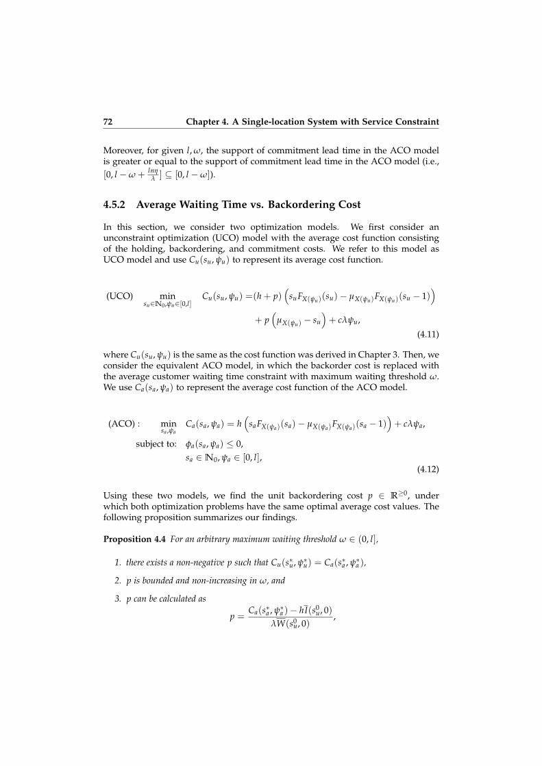
72 Chapter 4. A Single-location System with Service Constraint
Moreover, for given l, ω, the support of commitment lead time in the ACO modelis greater or equal to the support of commitment lead time in the ACO model (i.e.,[0, l −ω + lnη
λ ] ⊆ [0, l −ω]).
4.5.2 Average Waiting Time vs. Backordering Cost
In this section, we consider two optimization models. We first consider anunconstraint optimization (UCO) model with the average cost function consistingof the holding, backordering, and commitment costs. We refer to this model asUCO model and use Cu(su, ψu) to represent its average cost function.
(UCO) minsu∈N0,ψu∈[0,l]
Cu(su, ψu) =(h + p)(
suFX(ψu)(su)− µX(ψu)FX(ψu)(su − 1))
+ p(
µX(ψu) − su
)+ cλψu,
(4.11)
where Cu(su, ψu) is the same as the cost function was derived in Chapter 3. Then, weconsider the equivalent ACO model, in which the backorder cost is replaced withthe average customer waiting time constraint with maximum waiting threshold ω.We use Ca(sa, ψa) to represent the average cost function of the ACO model.
(ACO) : minsa ,ψa
Ca(sa, ψa) = h(
saFX(ψa)(sa)− µX(ψa)FX(ψa)(sa − 1))+ cλψa,
subject to: φa(sa, ψa) ≤ 0,sa ∈N0, ψa ∈ [0, l],
(4.12)
Using these two models, we find the unit backordering cost p ∈ R≥0, underwhich both optimization problems have the same optimal average cost values. Thefollowing proposition summarizes our findings.
Proposition 4.4 For an arbitrary maximum waiting threshold ω ∈ (0, l],
1. there exists a non-negative p such that Cu(s∗u, ψ∗u) = Ca(s∗a , ψ∗a ),
2. p is bounded and non-increasing in ω, and
3. p can be calculated as
p =Ca(s∗a , ψ∗a )− hI(s0
u, 0)λW(s0
u, 0),

4.5 Comparisons 73
where I(s0u, 0) and W(s0
u, 0) are the average inventory and customer waiting timeunder control policy (s0
u, 0).
We refer to Appendices 4.7.10, 4.7.11, and 4.7.12 for the proofs. From Subsection4.3.3.1, we know that when the maximum waiting threshold is small enough orclose to zero, then s∗a = 0 and ψ∗a = l −ω. Consequently, Ca(s∗a , ψ∗a ) = λc(l −ω). Inthis case, there is a negative linear correlation between ω and p as follows.
p =λc(l −ω)− hI(s0
u, 0)λW(s0
u, 0)(4.13)
According to Expression (4.13), p is linearly decreasing in ω. For two parametersettings shown in Figure 4.11, we plot the behavior of p as a function of ω. As it hasbeen shown by two dotted vertical lines, in both cases there is a linear relationshipbetween p and ω.
0 0.5 1 1.5 2 2.5 3 3.5 40
0.5
1
1.5
2
2.5
3
3.5
4
Maximun waiting threshold (ω)
p($ t)
λ = 9, h = 40, c = 0.7, l = 10
0 0.5 1 1.5 2 2.5 3 3.5 40
2
4
6
8
10
12
14
16
Maximun waiting threshold (ω)
p($ t)
λ = 3, h = 15, c = 2.2, l = 10
Figure 4.11: The equivalent unit backordering cost p to the waiting time threshold ω
Notice that by considering commitment lead time, it is always possible to find anequivalent unit backoredering cost such that a desired maximum waiting thresholdon average customer waiting time is guaranteed.
4.5.3 The Value of the Commitment Lead Time
We investigate the value of considering or ignoring the commitment lead time whenaverage customer waiting time is considered as a service measure. For this purpose,we study Ca(s, ψ) and Ca(s, 0). Both models are constraint optimization models. Inthe latter case, commitment lead time is not a decision variable anymore. Sincein both models finding analytical results is difficult, for a fixed parameter setting,we illustrate the optimal value of cost functions in terms of the maximum waitingthreshold ω.

74 Chapter 4. A Single-location System with Service Constraint
0 0.2 0.4 0.6 0.8 1 1.2 1.4 1.6 1.8 2 2.2 2.4 2.6 2.8 3 3.2 3.4 3.6 3.8 40
25
50
75
100
125
150
Maximum waiting threshold (ω)
Opt
imal
cost
λ = 3, h = 15, c = 2.2, l = 10
Ca(s∗, 0)Ca(s∗, ψ∗)
Figure 4.12: The optimal cost values with and without commitment lead time
As it is seen in Figure 4.12, considering commitment lead time always gives a loweror equal optimal average cost compared to ignoring the commitment lead timecase (i.e., Ca(s∗, ψ∗) is a lower bound for Ca(s∗, 0)). Moreover, Ca(s∗, ψ∗) givessignificantly lower optimal average cost when the maximum waiting threshold ω issmall enough. Hence, when the firm expects negligible average customer waitingtime or very quick response, the commitment lead time plays a significant role inthe optimal control policy.
4.6. Conclusion
In this chapter, we considered a firm which faces a Poisson customer demandand uses a base-stock policy to replenish its inventories from an outside sourcewith a deterministic lead time. The system operates under a preorder strategy,in which customers place their order ahead of their actual need based on apredetermined time window called commitment lead time. In turn, the firm paysthe customer a bonus based on the length of the commitment lead time, which iscalled commitment cost. The firm manager aims to find the optimal control policyas a combination of the base-stock level and commitment lead time such that a long-run average total cost consisting of holding and commitment costs is minimizedsubject to a time-based service constraint. We studied this problem with two time-based service measures; average customer waiting time and individual customerwaiting time. For the first measure, we put a maximum waiting threshold on theaverage customer waiting time. For the second, we formed a chance constraintconsisting of a service level as well as the maximum waiting threshold. Since wedealt with two Constraint, Mixed-integer, Nonlinear Programs (C-MINLP), findingclosed-form solutions are not possible. Instead, we proposed exact and heuristicoptimization algorithms for each optimization model. Using a comprehensive

4.6 Conclusion 75
numerical experiment we showed that the heuristic algorithms perform quite well.
We observed that when commitment lead time and time-based service measureswith positive maximum waiting threshold are taken into account, the optimalcommitment lead time is not a bang-bang policy, anymore. However, for η−servicelevel type of fill rate (i.e., on-time fulfillment), the optimal commitment lead timetakes a bang-bang form. In other words, it is either equal to zero or l + lnη
λ . Wederived the exact distribution probability of customer waiting time in terms ofsystem parameters and control policy. We show that the commitment lead time notonly increases the service level (i.e., the likelihood of meeting a customer demandup to a maximum waiting threshold) but also decreases the possible maximumwaiting time. We showed that the optimal cost value is bounded and non-increasingin the maximum waiting threshold. We found that the commitment lead time playsa significant role in the determination of the optimal control policy when eitherthe maximum waiting threshold is small enough (e.g., close to zero) or the servicelevel is high enough (e.g., close to one). In other words, when the firm wants toprovide a quicker response to a higher percentage of the customers, the value ofcommitment lead time in terms of cost reduction is more highlighted. Moreover,we considered an unconstraint optimization model with backordering cost and itsequivalent constraint optimization model with the average waiting time constraint.We calculated equivalent unit backordering cost such that both models have thesame optimal cost. We found a negative relationship between unit backorderingcost and maximum waiting threshold. When commitment lead time is taken intoaccount, the equivalent unit backordering cost is always bounded above.
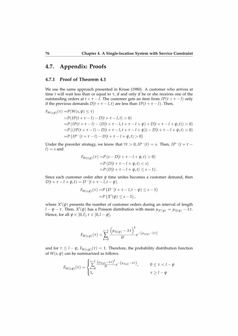
76 Chapter 4. A Single-location System with Service Constraint
4.7. Appendix: Proofs
4.7.1 Proof of Theorem 4.1
We use the same approach presented in Kruse (1980). A customer who arrives attime t will wait less than or equal to τ, if and only if he or she receives one of theoutstanding orders at t + τ − l. The customer gets an item from IP(t + τ − l) onlyif the previous demands D[t + τ − l, t) are less than IP(t + τ − l). Then,
FW(s,ψ)(τ) =P(W(s, ψ) ≤ τ)
=P(IP(t + τ − l)− D[t + τ − l, t) > 0)=P (IP(t + τ − l)− (D[t + τ − l, t + τ − l + ψ) + D[t + τ − l + ψ, t)) > 0)=P ((IP(t + τ − l)− D[t + τ − l, t + τ − l + ψ))− D[t + τ − l + ψ, t) > 0)
=P(
IP−(t + τ − l)− D[t + τ − l + ψ, t) > 0)
Under the preorder strategy, we know that ∀t > 0, IP−(t) = s. Then, IP−(t + τ −l) = s and
FW(s,ψ)(τ) =P (s− D[t + τ − l + ψ, t) > 0)
=P (D[t + τ − l + ψ, t) < s)=P (D[t + τ − l + ψ, t) ≤ s− 1) .
Since each customer order after ψ time unites becomes a customer demand, thenD[t + τ − l + ψ, t) = D−[t + τ − l, t− ψ).
FW(s,ψ)(τ) =P(
D−[t + τ − l, t− ψ) ≤ s− 1)
=P(X′(ψ) ≤ s− 1
),
where X′(ψ) presents the number of customer orders during an interval of lengthl − ψ− τ. Then, X′(ψ) has a Poisson distribution with mean µX′(ψ) = µX(ψ) − λτ.Hence, for all ψ ∈ [0, l], τ ∈ [0, l − ψ],
FW(s,ψ)(τ) =s−1
∑k=0
(µX(ψ) − λτ
)k
k!e−(µX(ψ)−λτ)
and for τ ≤ l − ψ, FW(s,ψ)(τ) = 1. Therefore, the probability distribution functionof W(s, ψ) can be summarized as follows.
FW(s,ψ)(τ) =
s−1∑
k=0
(µX(ψ)−λτ)k
k! e−(µX(ψ)−λτ), 0 ≤ τ < l − ψ
1, τ ≥ l − ψ

4.7 Appendix: Proofs 77
For the probability mass of the customer waiting time at zero, we can write
PW(s,ψ)(0) = FW(s,ψ)(0) =s−1
∑k=0
(µX(ψ)
)k
k!e−µX(ψ)
Let fW(s,ψ)(τ) be the probability density function of W(s, ψ). Then, for all 0 <
τ < l − ψ, fW(s,ψ)(τ) = ddτ FW(s,ψ)(τ). for ease of calculation, let us introduce
Poisson random variable Y(τ, ψ) with mean µX(ψ) − λτ. Then, for all 0 < τ <
l − ψ, FW(s,ψ)(τ) = FY(τ,ψ)(s − 1). From Appendix 3.6.1, we knowdFY(τ,ψ)(s−1)
dτ =
λPY(τ,ψ)(s − 1). Hence, for all 0 < τ < l − ψ, fW(s,ψ)(τ) = λPY(τ,ψ)(s − 1);otherwise, fW(s,ψ)(τ) = 0. Therefore, the probability density function of W(s, ψ)can be summarized as follows.
fW(s,ψ)(τ) =
λ(µX(ψ)−λτ)
s−1
(s−1)! e−(µX(ψ)−λτ), 0 < τ < l − ψ
0, otherwise
4.7.2 Proof of Lemma 4.1
We first show that for all s ∈ N0,dFW(s,ψ)(τ)
dψ ≥ 0. Based on Appendix 4.7.1, forall τ ∈ (0, l − ψ), FW(s,ψ)(τ) = FY(τ,ψ)(s− 1), where FY(τ,ψ)(s− 1) is the cumulativedistribution of Poisson at s− 1 with mean µY(τ,ψ) = µX(ψ)− λτ. Also, from Chapter
3, we know thatdFY(τ,ψ)(s−1)
dψ = λPY(τ,ψ)(s− 1) ≥ 0. Then, for all τ ∈ (0, L),
dFW(s,ψ)(τ)
dψ =dFY(τ,ψ)(s−1)
dψ = λPY(τ,ψ)(s− 1) ≥ 0.
Then, for all ψ ∈ [0, l], we show that ∆sFW(s,ψ)(τ) ≥ 0. To do so, we show that∆sFY(τ,ψ)(s− 1) ≥ 0. By calculating FY(τ,ψ)(s) = FY(τ,ψ)(s− 1) + PY(τ,ψ)(s), we canwrite ∆sFW(s,ψ)(τ) = ∆sFY(τ,ψ)(s− 1) = FY(τ,ψ)(s)− FY(τ,ψ)(s− 1) = PY(τ,ψ)(s) ≥ 0.

78 Chapter 4. A Single-location System with Service Constraint
4.7.3 Proof of Proposition 4.1
Based on Theorem 4.1, the expected waiting time is calculated as follows.
W(s, ψ) = E{W(s, ψ)} =∫ L
0τ fW(s,ψ)(τ)dτ =
∫ l−ψ
0τλ
(µX(ψ) − λτ
)s−1
(s− 1)!e−(µX(ψ)−λτ)dτ
=∫ l−ψ
0τλs (l − ψ− τ)s−1
(s− 1)!e−λ(l−ψ−τ)dτ
=λs
(s− 1)!
∫ l−ψ
0τ(l − ψ− τ)s−1e−λ(l−ψ−τ)dτ
By substituting l − ψ− τ = x, then τ = l − ψ− x and dτ = −dx.
=λs
(s− 1)!
∫ l−ψ
0(l − ψ− x)xs−1e−λxdx.
By substituting λx = y, then x = 1λ y and dx = 1
λ dy.
=λs
(s− 1)!
∫ µX(ψ)
0
(l − ψ− y
λ
) ( yλ
)s−1e−y 1
λdy =
1λ(s− 1)!
∫ µX(ψ)
0
(µX(ψ) − y
)ys−1e−ydy
=1
λ(s− 1)!
(µX(ψ)
∫ µX(ψ)
0ys−1e−ydy−
∫ µX(ψ)
0yse−ydy
),
(4.14)
where µX(ψ) = λ(l − ψ). Based on the definition of the upper incomplete gammafunction Γ(s, µX(ψ)) for positive integer s;
Γ(s, µX(ψ)) = (s− 1)!e−µX(ψ)
s−1
∑k=0
(µX(ψ)
)k
k!,
the lower incomplete gamma function γ(s, µX(ψ))
γ(s, µX(ψ)) =∫ µX(ψ)
0ys−1e−ydy,
the ordinary gamma function Γ(s) = (s− 1)!, and their relationship as γ(s, µX(ψ)) =
Γ(s)− Γ(s, µX(ψ)), we can write
∫ µX(ψ)
0ys−1e−ydy = (s− 1)!
1− e−µX(ψ)
s−1
∑k=0
(µX(ψ)
)k
k!
(4.15)
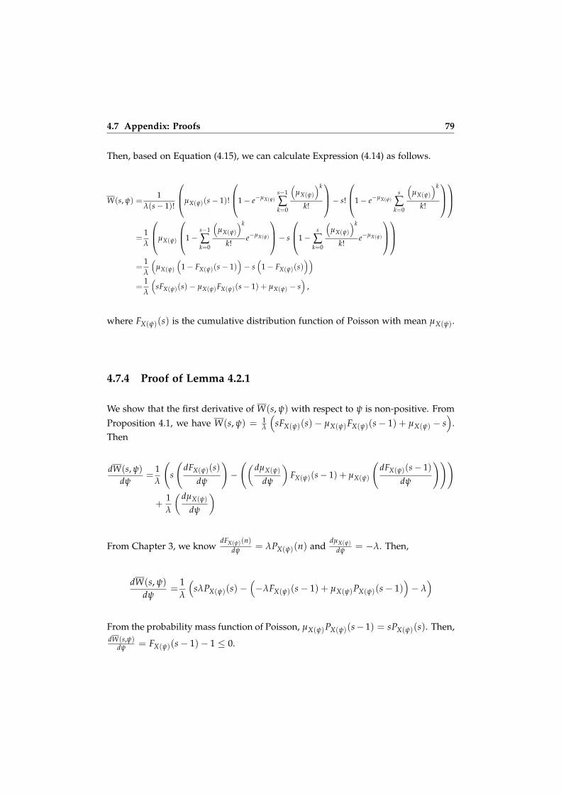
4.7 Appendix: Proofs 79
Then, based on Equation (4.15), we can calculate Expression (4.14) as follows.
W(s, ψ) =1
λ(s− 1)!
µX(ψ)(s− 1)!
1− e−µX(ψ)
s−1
∑k=0
(µX(ψ)
)k
k!
− s!
1− e−µX(ψ)
s
∑k=0
(µX(ψ)
)k
k!
=1λ
µX(ψ)
1−s−1
∑k=0
(µX(ψ)
)k
k!e−µX(ψ)
− s
1−s
∑k=0
(µX(ψ)
)k
k!e−µX(ψ)
=1λ
(µX(ψ)
(1− FX(ψ)(s− 1)
)− s
(1− FX(ψ)(s)
))=
1λ
(sFX(ψ)(s)− µX(ψ)FX(ψ)(s− 1) + µX(ψ) − s
),
where FX(ψ)(s) is the cumulative distribution function of Poisson with mean µX(ψ).
4.7.4 Proof of Lemma 4.2.1
We show that the first derivative of W(s, ψ) with respect to ψ is non-positive. FromProposition 4.1, we have W(s, ψ) = 1
λ
(sFX(ψ)(s)− µX(ψ)FX(ψ)(s− 1) + µX(ψ) − s
).
Then
dW(s, ψ)
dψ=
1λ
(s
(dFX(ψ)(s)
dψ
)−((dµX(ψ)
dψ
)FX(ψ)(s− 1) + µX(ψ)
(dFX(ψ)(s− 1)
dψ
)))
+1λ
(dµX(ψ)
dψ
)
From Chapter 3, we knowdFX(ψ)(n)
dψ = λPX(ψ)(n) anddµX(ψ)
dψ = −λ. Then,
dW(s, ψ)
dψ=
1λ
(sλPX(ψ)(s)−
(−λFX(ψ)(s− 1) + µX(ψ)PX(ψ)(s− 1)
)− λ
)
From the probability mass function of Poisson, µX(ψ)PX(ψ)(s− 1) = sPX(ψ)(s). Then,dW(s,ψ)
dψ = FX(ψ)(s− 1)− 1 ≤ 0.

80 Chapter 4. A Single-location System with Service Constraint
4.7.5 Proof of Lemma 4.2.2
We show that for all ψ ∈ [0, l], ∆sW(s, ψ) = W(s + 1, ψ)−W(s, ψ) ≤ 0. First, wecalculate W(s + 1, ψ) as follows.
W(s + 1, ψ) =1λ
((s + 1)FX(s + 1, ψ)− µX(ψ)FX(ψ)(s) + µX(ψ) − s− 1
)=
1λ
(sFX(ψ)(s) + FX(ψ)(s) + (s + 1)PX(ψ)(s + 1)− µX(ψ)FX(ψ)(s− 1)
)+
1λ
(−µX(ψ)PX(ψ)(s) + µX(ψ) − s− 1
)=W(s, ψ) +
1λ
(FX(ψ)(s) + (s + 1)PX(ψ)(s + 1)− µX(ψ)PX(ψ)(s)− 1
)From the probability mass function of Poisson, µX(ψ)PX(ψ)(s) = (s + 1)PX(ψ)(s +
1). Then, W(s + 1, ψ) = W(s, ψ) + 1λ
(FX(ψ)(s)− 1
). Hence, ∆sW(s, ψ) =
1λ
(FX(ψ)(s)− 1
)≤ 0.
4.7.6 Proof of Lemma 4.3
First, we show that for all ψ ∈ [0, l], the first forward difference of φa(s, ψ) is non-positive. By rewriting φa(s, ψ) as φa(s, ψ) = λ(W(s, ψ) − ω) and using proof ofLemma 4.2.2, we have
∆sφa(s, ψ) = λ(∆sW(s, ψ)−ω) = λ
(1λ(FX(ψ)(s)− 1)
)= FX(ψ)(s)− 1
Since for all s ∈ N0 and ψ ∈ [0, l] we have ∆sφa(s, ψ) = FX(ψ)(s) − 1 ≤ 0, thenφa(s, ψ) is non-increasing in s.
Then, we show that for all s ∈ N0, the first derivative of φ(s, ψ) is non-positive.Using proof of Lemma 4.2.1, we can write
ddψ
φa(s, ψ) =λ
(d
dψW(s, ψ)−ω
)= λ(FX(ψ)(s− 1)− 1)
Since for all s ∈ N0, ψ ∈ [0, l] and λ > 0, we have ddψ φa(s, ψ) ≤ 0, then φa(s, ψ) is
non-increasing in ψ.
4.7.7 Proof of Proposition 4.2.1
Let ω1, ω2 ∈ [0, l] and without loss of generality ω1 < ω2. Then, there existsδ > 0 such that ω2 = ω1 + δ. Let φω1
a (s, ψ) and φω2a (s, ψ) indicate constraints

4.7 Appendix: Proofs 81
corresponding to ω1 and ω2, respectively. Knowing φa(s, ψ) = λ(W(s, ψ) − ω),then
φω2a (s, ψ) =λ(W(s, ψ)−ω2) = λ(W(s, ψ)− (ω1 + δ))
=λ(W(s, ψ)−ω1)− λδ = φω1a (s, ψ)− λδ.
Hence, for a given s ∈N0 and ψ ∈ [0, l], φω2a (s, ψ) < φω1
a (s, ψ). Since φa(s, ψ) is non-increasing in s, then setting φω2
a (s, ψ) = 0 and φω1a (s, ψ) = 0 result in |Θω2
a | ≤ |Θω1a |.
Since φa(s, ψ) is non-increasing in ψ, for all s’s correspond to breakpoints belongto Θω2
a , we have ψω2s < ψω1
s . Also, Ca(s, ψ) is increasing in ψ. Then, Ca(s, ψω2s ) <
Ca(s, ψω1s ). Consequently,
mins
Ca(s, ψω2s ) < min
sCa(s, ψω1
s )
andCω2
a (s∗, ψ∗) < Cω1a (s∗, ψ∗).
Therefore, Ca(s∗, ψ∗) is decreasing in ω.
4.7.8 Proof of Proposition 4.2.2
Let Ca(s∗, ψ∗) be the optimal cost value of the ACO model. Then, for all thebreakpoints ψs ∈ Θa, we have Ca(s∗, ψ∗) ≤ Ca(s, ψs). Also, in the ACO model,ψ0 = l −ω ∈ Θa. Then, Ca(s∗, ψ∗) ≤ Ca(0, l −ω) = cλ(l −ω) = cµX(ω).
4.7.9 Proof of Proposition 4.3
Let Cc(s∗, ψ∗) be the optimal cost value of the CCO model. Then, for all thebreakpoints ψs ∈ Θc, we have Cc(s∗, ψ∗) ≤ Cc(s, ψs). Also, in the CCO model,ψ1 = l −ω + lnη
λ ∈ Θc. Then,
Cc(s∗, ψ∗) ≤ Ca(1, l −ω +lnη
λ) =
hη
e−µX(ω) + c(
lnη + µX(ω)
).
4.7.10 Proof of Proposition 4.4.1
In the UCO model, for p = 0, we have (s∗u, ψ∗u) = (0, 0) and Cu(s∗u, ψ∗u) = 0. Also,for p > 0 we know from Chapter 3, there exists c0 such that for all c ∈ [0, c0] wehave (s∗u, ψ∗u) = (0, l) and for all c ∈ [c0,+∞) we have (s∗u, ψ∗u) = (s0
u, 0). Recall thatc0 is increasing in p. For a given c, by increasing p starting from zero, we reach ap0 such that c0 = c and for all p ≤ p0 (i.e., c0 ≤ c) we have (s∗u, ψ∗u) = (s0
u, 0). Thisimplies that Cu(s0
u, 0) ≤ Cu(0, l) = cµX(0). Based on Proposition 4.2.2, we know that

82 Chapter 4. A Single-location System with Service Constraint
Ca(s∗a , ψ∗a ) ≤ cµX(ω). Hence, for all ω ∈ (0, l], Ca(s∗a , ψ∗a ) < cµX(0). Since Cu(s∗u, ψ∗u)is a continuous function in p and both functions (i.e., Cu(s∗u, ψ∗u) and Ca(s∗a , ψ∗a ))have the same range, for a given Ca(s∗a , ψ∗a ), there exists a p ∈ [0, p0] such thatCu(s∗u, ψ∗u) = Ca(s∗a , ψ∗a ).
4.7.11 Proof of Proposition 4.4.2
Based on the proof of Proposition (4.4.1), the equivalent optimal cost value in theUCO model always happens at (s0, 0). Then, Cu(s∗u, ψ∗u) = Cu(s0
u, 0) = hI(s0, 0) +pλW(s0, 0) which is a strictly continuous function in p. Based on Proposition 4.2.2,we know that Ca(s∗a , ψ∗a ) ≤ cλ(l − ω) = cµX(ω). Hence, by putting Cu(s∗u, ψ∗u) =
Ca(s∗a , ψ∗a ), we can conclude that Cu(s∗u, ψ∗u) ≤ cµX(ω) and
p ≤cµX(ω) − hI(s0, 0)
λW(s0, 0)
Therefore, the equivalent p is bounded.From Proposition (4.2.1), Ca(s∗a , ψ∗a ) is non-increasing in ω. Knowing that Cu(s0
u, 0) isstrictly increasing in p and Cu(s0
u, 0) = Ca(s∗a , ψ∗a ), then p should be non-increasingin ω, and vice versa.
4.7.12 Proof of Proposition 4.4.3
Based on the proof of Proposition 4.4.1, the equivalent optimal cost value in theUCO model always happens at (s0, 0). Then, Cu(s∗u, ψ∗u) = Cu(s0
u, 0) = hI(s0, 0) +pλW(s0, 0) which is a continuous function in p. By putting Cu(s0
u, 0) = Ca(s∗a , ψ∗a ),we have
p =Ca(s0
a, ψ∗a )− hI(s0u, 0)
λW(s0u, 0)
.
4.7.13 Proof of Lemma 4.4
We first show that for all s ∈N0, dφc(s,ψ)dψ ≤ 0. From φc(s, ψ) = η − F(ω,τ)(s− 1), we
can writedφc(s, ψ)
dψ=
dF(ω,τ)(s− 1)dψ
= −λP(ω,τ)(s− 1) ≤ 0.
Then, for all ψ ∈ [0, l], we show that ∆sφc(s, ψ) ≤ 0. By calculating φc(s + 1, ψ) =η − F(ω,τ)(s) = η − F(ω,τ)(s− 1)− F(ω,τ)(s) = φc(s + 1, ψ)− P(ω,τ)(s), we can write
∆sφc(s, ψ) = φc(s + 1, ψ)− φc(s, ψ) = −P(ω,τ)(s) ≤ 0.

4.7 Appendix: Proofs 83
4.7.14 The Heuristic Algorithm for ACO Model
Procedure 1 The heuristic algorithm for ACO model
Input: λ, h, c, l ∈ R+, ω ∈ [0, l]Output: Finding optimal control policy (s∗, ψ∗), and C(s∗, ψ∗)
1: Set s = 0, calculate ψ0 = l −ω, and compute C(0, ψ0) = cµX(ω)
2: Set ψs0 = 0, find s0 = inf{s ∈N0 : φa(s, 0) ≤ 0}, and compute
C(s0, 0) = hs0 − hc
C(0, ψ0)
.3: Find ψs0−1 = {ψ ∈ [0, l] : φa(s0 − 1, ψ) = 0} and compute
C(s0 − 1, ψs0−1) = C(s0, 0) + λ(h + c)ψs0−1 − h
.4: Compare C(0, ψ0), C(s0, 0), and C(s0 − 1, ψs0−1) and consider the minimum
among them as optimal cost value and its corresponding (s, ψ) as the optimalcontrol policy.
4.7.15 The Heuristic Algorithm for CCO Model
Procedure 2 The heuristic algorithm for CCO model
Input: λ, h, c, l ∈ R+, ω ∈ [0, l], η ∈ (0, 1)Output: Finding optimal control policy (s∗, ψ∗), and C(s∗, ψ∗)
1: Set s = 1, find ψ1 = l −ω + lnηλ , and compute C(1, ψ1).
2: Set ψs0 = 0, calculate s0 = 1 + dF−1Y(ω,0)(η)e, and compute C(s0, 0).
3: Find ψs0−1 = {ψ ∈ [0, l] : φc(s− 1, 0) = 0} and compute C(s0 − 1, ψs0−1).4: Compare C(1, ψ1), C(s0, 0), and C(s0 − 1, ψs0−1) and consider the minimum
value among them as optimal cost value and its corresponding (s, ψ) as theoptimal control policy.

84 Chapter 4. A Single-location System with Service Constraint
4.7.16 The Exact Optimization Algorithm for ACO Model
Procedure 3 The exact optimization algorithm for ACO model
Input: ε > 0, λ, h, c, l ∈ R+, ω ∈ [0, l]Output: Finding optimal control policy (s∗, ψ∗), and C(s∗, ψ∗)
1: s← 1, ψ← 02: φa(s, ψ) = sFX(ψ)(s)− µX(ψ)FX(ψ)(s− 1) + µX(ψ) − s− λω
3: Φa ← φa(s, ψ)4: while Φa > 0 do {finding s0}5: s← s + 16: φa(s, ψ) = sFX(ψ)(s)− µX(ψ)FX(ψ)(s− 1) + µX(ψ) − s− λω
7: Φa ← φa(s, ψ)8: end while9: s0 = s
10: C(s∗, ψ∗)← C(s0, ψ)11: s∗ ← s0, ψ∗ ← ψ12: Result(1, :) = [s0 ψ C(s∗, ψ∗)] {a matrix including all the breakpoints}13: for s = s0 − 1 to 0 do14: Stop← 0, n← 015: ψ(n) ← 016: while Stop = 0 do {finding ψs using Newton’s method}17: µX(ψ) = λ
(l − ψ(n)
)18: ψ(n+1) = ψ(n) − φa(s,ψ(n))
λ
(F
X(ψ(n))(s−1)−1
)19: if |ψ(n+1) − ψ(n)| < ε then20: break21: else22: n← n + 123: end if24: end while25: ψs ← ψ(n+1)
26: Result(s0 − s + 1, :) = [s ψs C(s, ψs)]27: if C(s, ψs) < C(s∗, ψ∗) then28: C(s∗, ψ∗)← C(s, ψs)29: s∗ ← s30: ψ∗ ← ψs31: end if32: end for
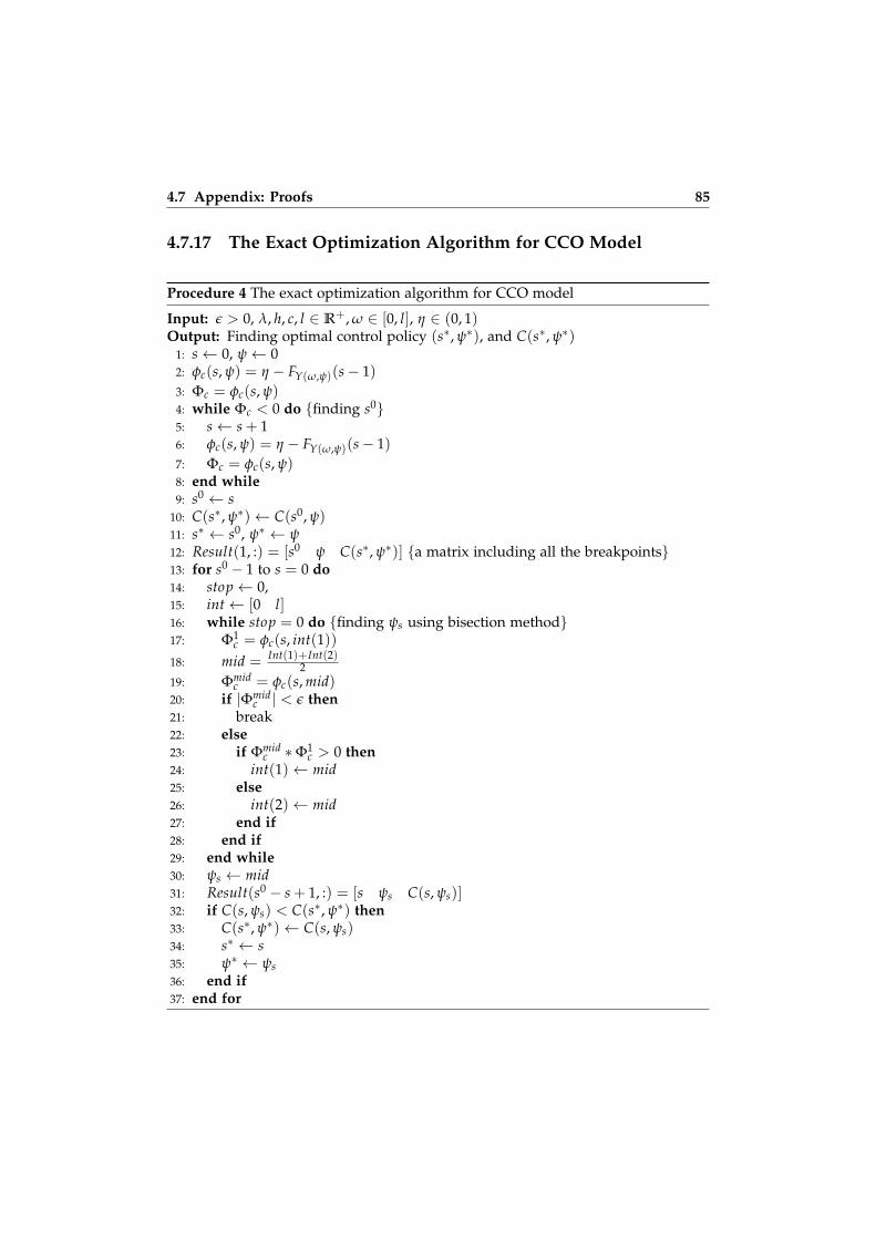
4.7 Appendix: Proofs 85
4.7.17 The Exact Optimization Algorithm for CCO Model
Procedure 4 The exact optimization algorithm for CCO model
Input: ε > 0, λ, h, c, l ∈ R+, ω ∈ [0, l], η ∈ (0, 1)Output: Finding optimal control policy (s∗, ψ∗), and C(s∗, ψ∗)
1: s← 0, ψ← 02: φc(s, ψ) = η − FY(ω,ψ)(s− 1)3: Φc = φc(s, ψ)4: while Φc < 0 do {finding s0}5: s← s + 16: φc(s, ψ) = η − FY(ω,ψ)(s− 1)7: Φc = φc(s, ψ)8: end while9: s0 ← s
10: C(s∗, ψ∗)← C(s0, ψ)11: s∗ ← s0, ψ∗ ← ψ12: Result(1, :) = [s0 ψ C(s∗, ψ∗)] {a matrix including all the breakpoints}13: for s0 − 1 to s = 0 do14: stop← 0,15: int← [0 l]16: while stop = 0 do {finding ψs using bisection method}17: Φ1
c = φc(s, int(1))18: mid = Int(1)+Int(2)
219: Φmid
c = φc(s, mid)20: if |Φmid
c | < ε then21: break22: else23: if Φmid
c ∗Φ1c > 0 then
24: int(1)← mid25: else26: int(2)← mid27: end if28: end if29: end while30: ψs ← mid31: Result(s0 − s + 1, :) = [s ψs C(s, ψs)]32: if C(s, ψs) < C(s∗, ψ∗) then33: C(s∗, ψ∗)← C(s, ψs)34: s∗ ← s35: ψ∗ ← ψs36: end if37: end for

5A Two-component, Single-end-product
ATO System with Commitment
5.1. Introduction
The companies in high-tech, car manufacturing and white goods industries aimto benefit from the strategic advantages of mass customization and delayeddifferentiation by attempting to delay the production of the end product until theyobtain better or complete demand information. Assemble-to-order (ATO) is a verypopular strategy that enables companies to reduce their customer response time bykeeping component inventories and delaying the final assembly of the end productsuntil the arrival of customer demand (Atan et al., 2017; Benjaafar and ElHafsi,2006). An ATO system with long component supply lead times has high componentavailability uncertainty. This implies high uncertainty in delivery time of the endproducts. Having high component inventory levels can increase the responsivenessof the system but results in high inventory holding cost. On the other hand, lowcomponent inventory levels lower the inventory holding cost but can result in aless responsive system. In order to achieve simultaneous improvement in both costand responsiveness, companies need to decrease the demand and supply mismatch.Having more accurate information on future customer demand, i.e., advance demandinformation (ADI), helps to reduce this mismatch.
In this study, we investigate the value of using the preorder strategy in managingthe assemble-to-order (ATO) systems. For this purpose, we consider a manu-facturer, who operates an ATO system with two components and a single endproduct. The manufacturer needs one unit of each component to assemble/producea unit of end product. The manufacturer keeps inventory of the components. The

88 Chapter 5. An ATO System
component inventories are replenished from two different uncapacitated suppliers.Continuous-review base-stock policies with deterministic replenishment lead timesare used to replenish component inventories. The assembly time is negligible.Customer demand occurs for the end product only and unsatisfied customerdemands are backordered. The manufacturer offers a preorder strategy to itscustomers and consequently, they are paid a commitment cost. The commitmentcost function is strictly increasing in the length of the commitment lead time. Themanufacturer aims to find the optimal component base-stock levels and the optimallength of the commitment lead time, which minimize the total long-run averagecost. This cost is the sum of the long-run average component inventory holding,backordering and commitment costs. We formulate the total long-run average costand answer the following questions:
1. When and how should the manufacturer use the preorder strategy?We find that the optimal commitment lead time is either zero or equalsthe replenishment lead time of one of the components. When the optimalcommitment lead time is equal to zero, the preorder strategy is not beneficial.The manufacturer should choose a strategy that is similar in spirit to a puremake-to-stock procurement strategy. In our context, this strategy is called buy-to-stock (BTS) strategy. When the optimal commitment lead time equals thelead time of the component with the shorter lead time, the optimal strategyfor this component is buy-to-order (BTO) (similar in spirit to a make-to-orderstrategy) and it is BTS for the other component. On the other hand, ifthe optimal commitment lead time equals the lead time of the componentwith the longer lead time, the optimal strategy is the BTO strategy for bothcomponents. We determine the conditions under which one of these threecases holds.
2. What are the characteristics of the optimal control policy?We show that the optimal base-stock policies are of “all-or-nothing” type. Thismeans that when the commitment lead time is zero, the corresponding base-stock levels are the solution of a well-known two-stage serial system withdeterministic lead times. This result follows from the fact that the assemblysystem can be reduced to an equivalent serial system (Rosling, 1989). Whenthe commitment lead time is longer than or equal to the replenishment leadtime of a component, the corresponding optimal base-stock level is zero.
Scholars have studied inventory management with ADI broadly from differentperspectives. Hariharan and Zipkin (1995) study a single location system withperfect ADI, continuous-review, deterministic replenishment lead time and Poissondemand. Assuming that the commitment lead time is the same for all customers,the authors prove the optimality of a base-stock policy. A similar setting has beenstudied in Chapter 3. Assigning a cost to commitment lead time, we characterize theoptimal preorder strategy and the corresponding optimal replenishment strategy.

5.2 Problem Formulation 89
More specifically, they prove the optimality of the bang-bang preorder and all-or-nothing replenishment strategies. Both studies consider a single location system.Our work uses these two studies as building blocks for characterizing the optimalpreorder and replenishment strategies for a more complicated assemble-to-ordersystem.
Our work belongs to the category of perfect ADI. We study the impact ofcommitment cost as a function of the commitment lead time in a two-component,single end product ATO system with perfect ADI. We consider continuous-reviewbase-stock policies, deterministic replenishment lead times and Poisson customerdemand. This study is most closely related to the study of Chapter 3. Differentfrom this study, in Chapter 3, we study a single-location inventory system. Weprove the optimality of bang-bang and all-or-nothing policies for the commitmentlead time and replenishment policy, respectively. Moreover, we introduce a unitcommitment cost threshold to make a decision on cost-effectiveness of ADI.
We contribute to the literature on ADI by providing the results for preorderstrategy in ATO systems with commitment cost. Song (1998) studies a preorderstrategy for a multi-component, multi-end-product ATO system. She investigatesthe customer satisfaction by considering order-fill-rate defined as the probabilityof satisfying an arbitrary demand within a predetermined time window. Differentform Song, we investigate the preorder strategy under the consideration of thecommitment cost. We identify the conditions under which having informationon future customer demand helps ATO systems in reducing component inventorylevels without sacrificing high service levels. Not only the manufacturers of thesesystems but also their customers, who provide information on the timing andquality of their future demand, benefit from the preorder strategy. Manufacturers ofATO systems can reduce their inventory levels but still provide high-quality serviceto their customers. Hence, many companies in high-tech, car manufacturing andwhite good industry can benefit from the results of this study.
The remainder of this chapter is organized as follows. In Section 5.2, we formulateand analyze the ATO system with commitment lead time and derive the expressionfor the long-run average cost function. In Section 5.3, we determine the optimalreplenishment and preorder strategies. In Section 5.4, we provide numericalexamples. Finally, in section 5.5, we conclude the chapter. We defer the proofsto the Appendix 5.6.
5.2. Problem Formulation
We consider a manufacturer managing an ATO system with two components and asingle end product. One unit of each component is needed to produce one unitof the end product. We use index j = 1, 2 for the components. The assumethat the manufacturer uses continuous-review base-stock policies to replenish the

90 Chapter 5. An ATO System
component inventories from uncapacitated suppliers. To the best of our knowledge,the form of the optimal policy for such a system with commitment lead time isunknown. Therefore, we assume that the system operates in a centralized fashionunder a base-stock policy. We find the optimal policy under these assumptions.The base-stock level and the deterministic replenishment lead time for componentj are sj and lj, respectively (l2 ≤ l1). Since the component replenishment leadtimes are much longer than the assembly time, we neglect the assembly time andassume that assembly is instantaneous. Customer orders occur for the end productonly and describe a stationary Poisson process with a rate λ. Each customerorders a single unit. When a customer order occurs, supplier 1, with the longerreplenishment lead time, places a replenishment order. However, supplier 2, withshorter replenishment lead time, synchronizes its net inventory with supplier 1.
The manufacturer aims to investigate the profitability of a preorder strategy, whichrequires that customers place their orders ψ time units before their actual need.We say that the demand occurs ψ time units after the corresponding order. Wecall ψ commitment lead time and assume that ψ is continuous. The manufacturerpays a commitment cost c per commitment time unit to each customer. Hence,commitment cost per customer is cψ. In addition to the commitment cost, themanufacturer pays an inventory holding cost of hj per unit of component j pertime unit. The preorder strategy implies that there is a commitment to deliver eachcustomer order by the end of the commitment lead time ψ, otherwise, demandis backordered and a backordering cost of p per unit per time unit is paid to thecustomer. The customer does not accept delivery before the end of commitmentlead time since the product is not needed before then. The manufacturer’s objectiveis to find the commitment lead time, ψ, and the base-stock levels, s1 and s2, whichminimize the total long-run average cost.
In the rest of the chapter, without loss of generality, we name the component withthe longer replenishment lead time as component 1, i.e., j = 1 and the componentwith the shorter replenishment lead time as component 2, i.e., j = 2. Refer to Figure5.1 for the graphical representation of the ATO system with l1 ≥ l2.
∞
0
∞
0
1
2l2
l1
D ∼Poisson(λ)
Figure 5.1: An ATO system with two components and a single end product
Next, we derive the expression for the total long-run average cost. This requires
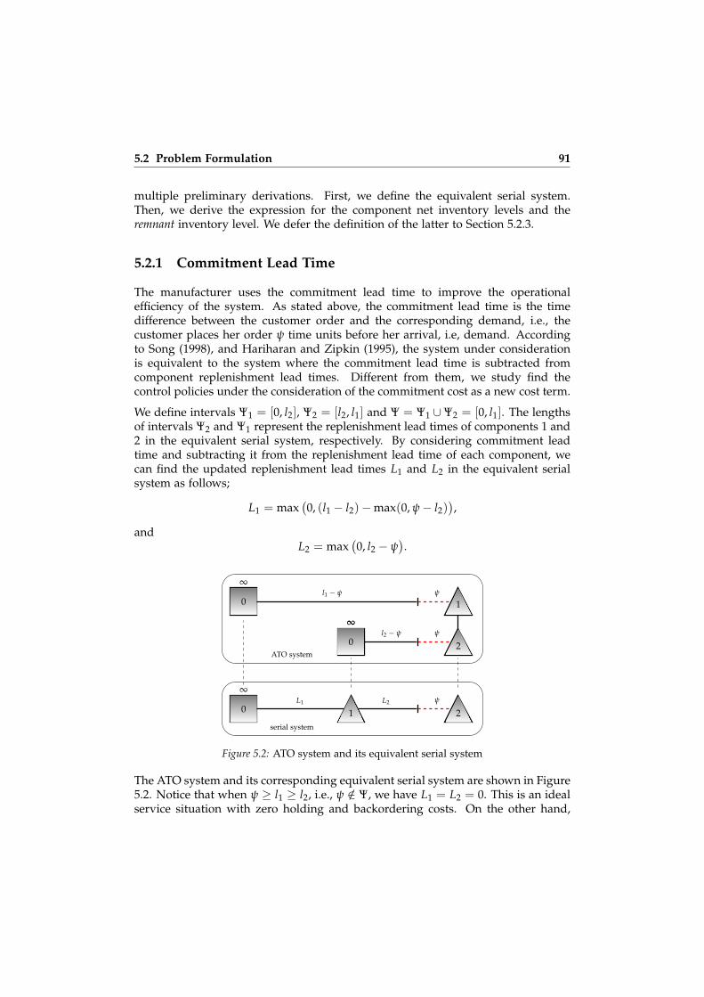
5.2 Problem Formulation 91
multiple preliminary derivations. First, we define the equivalent serial system.Then, we derive the expression for the component net inventory levels and theremnant inventory level. We defer the definition of the latter to Section 5.2.3.
5.2.1 Commitment Lead Time
The manufacturer uses the commitment lead time to improve the operationalefficiency of the system. As stated above, the commitment lead time is the timedifference between the customer order and the corresponding demand, i.e., thecustomer places her order ψ time units before her arrival, i.e, demand. Accordingto Song (1998), and Hariharan and Zipkin (1995), the system under considerationis equivalent to the system where the commitment lead time is subtracted fromcomponent replenishment lead times. Different from them, we study find thecontrol policies under the consideration of the commitment cost as a new cost term.
We define intervals Ψ1 = [0, l2], Ψ2 = [l2, l1] and Ψ = Ψ1 ∪Ψ2 = [0, l1]. The lengthsof intervals Ψ2 and Ψ1 represent the replenishment lead times of components 1 and2 in the equivalent serial system, respectively. By considering commitment leadtime and subtracting it from the replenishment lead time of each component, wecan find the updated replenishment lead times L1 and L2 in the equivalent serialsystem as follows;
L1 = max(0, (l1 − l2)−max(0, ψ− l2)
),
andL2 = max
(0, l2 − ψ
).
ATO system
serial system
∞
0
∞
0
1
2
l1 − ψ ψ
ψl2 − ψ
2
∞
0 1
∞
0
ψL2L1
Figure 5.2: ATO system and its equivalent serial system
The ATO system and its corresponding equivalent serial system are shown in Figure5.2. Notice that when ψ ≥ l1 ≥ l2, i.e., ψ /∈ Ψ, we have L1 = L2 = 0. This is an idealservice situation with zero holding and backordering costs. On the other hand,

92 Chapter 5. An ATO System
when ψ ∈ Ψ, there are two options for the pair (L1, L2) depending on whetherψ ∈ Ψ1 or ψ ∈ Ψ2. We have
(L1, L2) =
(l1 − l2, l2 − ψ) ψ ∈ Ψ1,(l1 − ψ, 0) ψ ∈ Ψ2,(0, 0) ψ /∈ Ψ.
From the first two options we observe that, depending on the length of commitmentlead time ψ ∈ Ψ, one of the component replenishment lead times depends on ψ. Ifψ ∈ Ψ1, L2 depends on ψ and if ψ ∈ Ψ2, L1 depends on ψ. Accordingly, we divideour analysis into two cases; when ψ ∈ Ψ1 and ψ ∈ Ψ2. In the former case we have atwo-stage serial inventory system, while in the latter case we have a single-locationinventory system, i.e., L2 = 0. It is important to remember that ψ is a decisionvariable. Hence, the optimal case depends on the system parameters.
5.2.2 Net Inventory Levels
The manufacturer manages the replenishment processes of both components.Hence, the inventory system is managed centrally; the manufacturer has all theinformation on component net inventory levels and can coordinate the replenish-ment processes to avoid having excess inventory of one component and out-of-stocksituation for the other component. The manufacturer would like to avoid suchimbalances to the extent possible.
For an assembly system with two components, the component with the longerlead time uses an ordinary base-stock policy. When a customer order occurs,a replenishment order for component 1 is placed. In this case, the inventoryposition of component 1, IP1(t) = IN1(t) + IO1(t) is not stationary. Let IP−1 (t) =IP1(t)−D(t, t+ψ] be the modified inventory position of component 1. If the systemstarts with IP−1 (0−) ≤ s1, we immediately order the difference, so that IP−1 (0) = s1.If IP−1 (0−) > s1, we order nothing until demand reduces IP−1 (t) to s. Once IP−1 (t)hits s1, it remains there from then on. This implies a one-for-one replenishment.
Let us define D(t1, t2] and D−(t1, t2] as the cumulative customer demand andcumulative customer order from time t1 to t2, respectively. Since under the preorderstrategy each customer order becomes customer demand after ψ time units, we canwrite D(t1, t2] = D−(t1 − ψ, t2 − ψ]. The conservation-of-flow law, implies that
IN1(t + l1) =IN1(t) + IO1(t)− D(t, t + l1]=IP1(t)− D(t, t + l1]=IP1(t)− (D(t, t + ψ] + D(t + ψ, t + l1])
=IP−1 (t)− D(t + ψ, t + l1]
=s1 − D−(t, t + l1 − ψ],
(5.1)
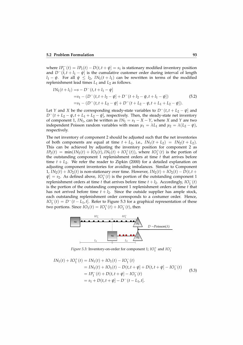
5.2 Problem Formulation 93
where IP−1 (t) = IP1(t)− D(t, t + ψ] = s1 is stationary modified inventory positionand D−(t, t + l1 − ψ] is the cumulative customer order during interval of lengthl1 − ψ. For all ψ ≤ l2, IN1(t + l1) can be rewritten in terms of the modifiedreplenishment lead times L1 and L2 as follows.
IN1(t + l1) =s− D−(t, t + l1 − ψ]
=s1 − (D−(t, t + l2 − ψ] + D−(t + l2 − ψ, t + l1 − ψ])
=s1 − (D−(t, t + L2 − ψ] + D−(t + L2 − ψ, t + L1 + L2 − ψ]).
(5.2)
Let Y and X be the corresponding steady-state variables to D−(t, t + L2 − ψ] andD−(t + L2 − ψ, t + L1 + L2 − ψ], respectively. Then, the steady-state net inventoryof component 1, IN1, can be written as IN1 = s1 − X − Y, where X and Y are twoindependent Poisson random variables with mean µ1 = λL1 and µ2 = λ(L2 − ψ),respectively.
The net inventory of component 2 should be adjusted such that the net inventoriesof both components are equal at time t + L2, i.e., IN1(t + L2) = IN2(t + L2).This can be achieved by adjusting the inventory position for component 2 asIP2(t) = min(IN2(t) + IO2(t), IN1(t) + IO+
1 (t)), where IO+1 (t) is the portion of
the outstanding component 1 replenishment orders at time t that arrives beforetime t + L2. We refer the reader to Zipkin (2000) for a detailed explanation onadjusting component inventories for avoiding imbalances. Similar to Component1, IN2(t) + IO2(t) is non-stationary over time. However, IN2(t) + IO2(t)− D(t, t +ψ] = s2. As defined above, IO+
1 (t) is the portion of the outstanding component 1replenishment orders at time t that arrives before time t + l2. Accordingly, IO−1 (t)is the portion of the outstanding component 1 replenishment orders at time t thathas not arrived before time t + l2. Since the outside supplier has ample stock,each outstanding replenishment order corresponds to a costumer order. Hence,IO−1 (t) = D−(t− L1, t]. Refer to Figure 5.3 for a graphical representation of thesetwo portions. Since IO1(t) = IO+
1 (t) + IO−1 (t), then
D ∼Poisson(λ)∞
∞
s1
s2
IO+1IO−1
L2L1
Figure 5.3: Inventory-on-order for component 1; IO+1 and IO−1
IN1(t) + IO+1 (t) = IN1(t) + IO1(t)− IO−1 (t)
= IN1(t) + IO1(t)− D(t, t + ψ] + D(t, t + ψ]− IO−1 (t)
= IP−1 (t) + D(t, t + ψ]− IO−1 (t)
= s1 + D(t, t + ψ]− D−(t− L1, t].
(5.3)

94 Chapter 5. An ATO System
Also, for component 2, we have
IN2(t) + IO2(t) = IN2(t) + IO2(t)− D(t, t + ψ] + D(t, t + ψ]
= (IN2(t) + IO2(t)− D(t, t + ψ]) + D(t, t + ψ]
= IP−2 (t) + D(t, t + ψ]
= s2 + D(t, t + ψ].
(5.4)
Then, by expanding the conservation-of-flow law for component 2 using Equations(5.3) and (5.4), we have
IN2(t + l2) = min(
IN2(t) + IO2(t), IN1(t) + IO+1 (t)
)− D(t, t + l2]
= min(s2 + D(t, t + ψ], s1 + D(t, t + ψ]− D−(t− L1, t]
)− D(t, t + l2]
= min(s2, s1 − D−(t− L1, t]
)− D−(t, t + L2 − ψ]
Then, the steady-state inventory level of component 2, IN2, can be written in termsof X and Y as IN2 = min(s2, s1 − X)−Y.
5.2.3 Remnant Inventory Levels
In an ATO system, when a customer order arrives, the ability of the manufacturerto satisfy the corresponding demand depends on the net inventory levels of thecomponents. The manufacturer is able to meet the demand at a specific point oftime if the minimum of the net inventories of both components is positive, i.e.,min(IN1, IN2) > 0; otherwise, the demand is backordered.
By definition of the base-stock policy, a customer order for the end product impliesorders for each individual component. If component inventory levels are positive,one unit of each component is dedicated to the specific customer order. We call thistype of inventories remnant inventory and use ∆Ij to represent the remnant inventorylevel of component j. In our setting, we have the remnant inventory only when onecomponent is available and another one is missing (de Kok, 2003). Hence, at anypoint in time, there can be at most one component type in remnant inventory. Thesteady-state remnant inventory level of each component can be calculated as
∆I1 = max(0, B2 − B1) = max(0, max(0,−IN2)−max(0,−IN1)),
and∆I2 = max(0, B1 − B2) = max(0, max(0,−IN1)−max(0,−IN2)).
Here, B1 and B2 are steady-state backorder levels for components 1 and 2,respectively. It is obvious that a delayed delivery of one component does notonly result in backordering cost of the end product but also can result in inventoryholding cost for the other component if it is already in stock as remnant inventory.Next, we determine the expected remnant inventory levels for both components.We define E{X} as the expectation of random variable X.

5.2 Problem Formulation 95
Proposition 5.1 The expected remnant inventory levels for an ATO system with twocomponents and Poisson customer demand for the end product are
E{∆I1} =s1−s2
∑x=0
(s1−x
∑y=s2+1
(y− s2)P2(y) + (s1 − s2 − x)(1− F2(s1 − x))
)P1(x),
E{∆I2} = 0.
Here, Fj(x) and Pj(x) are the cumulative distribution and probability mass functionsof a Poisson random variable with mean µj = λLj, respectively. Accordingto Proposition 5.1, when component inventories are controlled centrally by themanufacturer, the orders for component 2 can be synchronized with the orders forcomponent 1 such that E{∆I2} = 0. In addition, if s1 ≤ s2, the expected remnantinventory level of component 1 is zero, i.e., E{∆I1} = 0. Except for this case withs1 ≤ s2, even under a centralized control, the expected remnant inventory level ofcomponent 1 is positive. Under a decentralized control scheme both expectationscan be positive.
5.2.4 Long-run Average Cost
Having the expressions for the net inventory levels and the expected remnantinventory levels, we are ready to derive the expression for the long-run averagecost. For that purpose, we define Ij as on-hand inventory level of component jand B as the number of backorders of the end product. We use s to representthe base-stock level pair (s1, s2). Then, for an arbitrary base-stock level pair s andcommitment lead time ψ we can write the long-run average cost Ca(s, ψ) as follows
Ca(s, ψ) = E
{2
∑j=1
hj(
Ij + ∆I j)+ pB
}+ cλψ.
Note that we append the subscript a to indicate that this is the conventional costof an ATO system. Ca(s, ψ) is the sum of long-run average holding, backorderingand commitment costs. Holding cost of each component is comprised of on handinventory holding cost and remnant inventory holding cost. The manufacturerincurs backordering cost if a customer demand is satisfied more than ψ timeunits after the corresponding order is given. Finally, the manufacturer incurscommitment cost. It is important to note that the random variables Ij, ∆Ij andB depend on s and ψ. Our purpose in the remainder of this section is to rewrite theexpression for Ca(s, ψ) such that these dependencies are made explicit.
Firstly, we rewrite Ca(s, ψ) by using the following equalities; Ij = [INj]+, for
j = 1, 2, ∆I1 = max(0, [IN2]− − [IN1]
−), ∆I2 = max(0, [IN1]− − [IN2]
−) andB = max([IN1]
−, [IN2]−), where [x]+ = max(0, x) and [x]− = max(0,−x). We

96 Chapter 5. An ATO System
have
Ca(s, ψ) =h1(E{[IN1]
+}+ E
{max
(0, [IN2]
− − [IN1]−)})
+ h2(E{[IN2]
+}+ E
{max
(0, [IN1]
− − [IN2]−)})
+ pE{
max([IN1]−, [IN2]
−)}+ cλψ.
The first and second rows are expected holding costs for on-hand and remnantinventory levels of components 1 and 2, respectively. The third row is the sum ofexpected backordering and commitment costs. Next, we rely on simple algebra toobtain the following equivalent expression for Ca(s, ψ). We refer the reader to theAppendix 5.6.2 for the derivations.
Ca(s, ψ) =2
∑j=1
hjE{INj}+ (p + h1 + h2)E{
max([IN1]
−, [IN2]−)}+ cλψ. (5.5)
Rosling (1989) and Chen and Zheng (1994) show that a two-component, single endproduct ATO system can be reduced to an equivalent two-stage serial system withmodified replenishment lead times Li (refer to Figure 5.2). In the equivalent serialsystem, the local holding costs for stages 1 and 2 are h1 and h1 + h2, respectively.According to Shang and Song (2003) the long-run average cost of the serial systemcan be written as
Cs(s, ψ) =2
∑j=1
hjE{INj}+ (p + h1 + h2)E{[IN2]
−}+ cλψ.
Note that we use subscript s to indicate the long-run average cost of the equivalentserial system. Under a centralized control scheme, the expression for E {B}, asderived in the Appendix 5.6.3, is as follows:
E {B} = E{
max([IN1]
−, [IN2]−)} = E
{[IN2]
−} . (5.6)
Although all the terms of Cs(s, ψ) and Ca(s, ψ) look exactly the same, there is a smalldifference that results from the fact that in the ATO system there is no holding costfor in-transit inventory, while in the serial system the holding cost for items in-transit to stage 2 is included. Hence, the total cost of the serial system exceeds thetotal cost of the assembly system by h1λL2 (Zhang, 2006). Then, for an arbitraryψ ∈ Ψ, we have Ca(s, ψ) = Cs(s, ψ)− h1λL2. It is a well-known result that, for anarbitrary ψ ∈ Ψ, the total cost of the equivalent serial system Cs(s, ψ) can be derivedusing the recursive method proposed by Shang and Song (2003). By subtractingh1λL2 and applying some simple algebra we can rewrite the expression for Ca(s, ψ)in terms of system parameters and decision variables. See Appendix 5.6.4 for thedetails.

5.3 Characterization of the Optimal Control Policies 97
Ca(s, ψ) = µ1
(p−
((p + h1)F1(s1 − s2 − 1) + (p + h1 + h2)
s1−1
∑t=s1−s2
F2(s1 − t− 1)P1(t)
))
+ s1
(−p +
((p + h1)F1(s1 − s2) + (p + h1 + h2)
s1
∑t=s1−s2+1
F2(s1 − t)P1(t)
))
+ µ2
(p− (p + h1 + h2)
(F2(s2 − 1)F1(s1 − s2 − 1) +
s1−1
∑t=s1−s2
F2(s1 − t− 1)P1(t)
))
+ s2(p + h1 + h2)F1(s1 − s2)
(F2(s2)−
p + h1p + h1 + h2
)+ cλψ.
(5.7)
Recall that Fj(x) and Pj(x) are the cumulative distribution function and massprobability functions of Poisson distribution with mean µj. When ψ ∈ Ψ1, thenµ1 = λ(l1 − l2) and µ2 = λ(l2 − ψ). When ψ ∈ Ψ2, µ1 = λ(l1 − ψ) and µ2 = 0. As aresult, when ψ ∈ Ψj, Fj(x) and Pj(x) are independent of ψ.
5.3. Characterization of the Optimal Control Policies
In this section, we analyze the properties of the cost function Ca(s, ψ) andcharacterize the optimal control policies.
5.3.1 Optimization of the Component Base-stock Levels
For an arbitrary ψ ∈ Ψ, determining the base-stock levels which minimize Ca(s, ψ)is a well-known optimization problem in the multi-echelon inventory theoryliterature. We have
Ca(sψ, ψ) = mins
Ca(s, ψ),
where Ca(sψ, ψ) is a tight lower bound for Ca(s, ψ) over Ψ. sψ represents the optimalpair (sψ
1 , sψ2 ) corresponding to a ψ ∈ Ψ. To compute the optimal echelon base-stock
levels, two nested convex functions should be minimized. More specifically, for agiven ψ ∈ Ψ, we need to solve recursive optimization equations which have beenproposed by Shang and Song (2003). Knowing that the optimal base-stock levelsof a two-component ATO system are equal to the optimal echelon base-stock levelsof the equivalent serial system, we can formulate the following theorem, whichstates the inequalities that need to be satisfied by the optimal base-stock levels. Thesimilar results for a two-echelon divergent system under discrete demand can befound in Dogru et al. (2009).

98 Chapter 5. An ATO System
Theorem 5.1 In a two-component ATO system with a given commitment lead time ψ ∈ Ψ,the optimal base-stock levels of components 1 and 2 are two non-negative integers sψ
1 andsψ
2 , which satisfy the inequalities
F2(sψ2 − 1) <
p + h1
p + h1 + h2≤ F2(s
ψ2 ),
andΠ1(s
ψ1 − 1, sψ
2 ) <p
p + h1 + h2≤ Π1(s
ψ1 , sψ
2 ),
where Fj(x) and Pj(x) are the cumulative distribution and probability mass functions of aPoisson random variable with mean µj = λLj and
Π1(x, y) =(
p + h1
p + h1 + h2
)F1(x− y) +
x
∑n=x−y+1
F2(x− n)P1(n).
We refer the reader to Appendix 5.6.5 for the proof. Theorem 5.1 states that theoptimal component base-stock levels depend on the commitment lead time. Foreach value of ψ, obtaining the optimal base-stock levels needs two consecutive steps.First, the optimal base-stock level of component 2, sψ
2 should be calculated, andthen by using this value in the second inequality, the optimal base-stock level ofcomponent 1, sψ
1 is calculated.
We would like to note that, when ψ ∈ Ψ2, we have µ2 = 0 and sψ2 = 0. Hence, when
ψ ∈ Ψ2 the manufacturer relies on a buy-to-order (BTO) strategy for component 2.In this case, Expression (5.7) reduces to
Ca((s1, 0), ψ) =µ1(p− (p + h1)F1(s1 − 1)) + s1(−p + (p + h1)F1(s1)) + cλψ.
Ca((s1, 0), ψ) represents the long-run average cost of a single-location inventorysystem. We refer to Chapter 3 for detailed analysis of the single-location systemwith commitment lead time.
With the next result, we prove the behavior of the optimal base-stock levels withrespect to the commitment lead time.
Theorem 5.2 The optimal base-stock level of component j, sψj , is a piecewise-constant and
non-increasing function of ψ ∈ Ψ for j = 1, 2.
According to Theorem 5.2, the manufacturer can operate with less inventory ifcommitment lead time gets longer. In fact, for a sufficiently long commitment lead,the manufacturer can optimize his long-run average cost by setting both componentbase-stock levels to zero. This would imply using a buy-to-order (BTO) policy. In

5.3 Characterization of the Optimal Control Policies 99
0 0.5 1 1.5 2 2.5 3 3.5 4 4.5 5 5.5 6 6.5 7 7.5 80
1
2
3
4
Commitment lead time (ψ)
Base
-sto
ckle
vel
λ = 0.4, h = [5, 7], p = 20, l = [8, 5], c = 6
sψ1
sψ2
Figure 5.4: An illustration of the optimal base-stock levels in terms of commitment leadtime
Figure 5.4, we illustrate how the optimal component base-stock levels change withrespect to the commitment lead time.
Next, we are interested in the behavior of the average cost function with respectto the commitment lead time. In Figure 5.5, for a specific parameter setting withλ = 0.4, h = [5, 7], p = 20, l = [8, 5] and c = 6, we draw the average cost function formultiple base-stock level pairs. We also indicate the tight lower bound of these costfunctions. This tight lower bound is Ca(sψ, ψ). This is the function that needs tominimized for obtaining the optimal commitment lead time. Note that the functionCa(sψ, ψ) does not have a well-defined behavior. This is why finding the optimalcommitment lead time requires a different approach.
0 0.5 1 1.5 2 2.5 3 3.5 4 4.5 5 5.5 6 6.5 7 7.5 819
20
21
22
23
24
25
26
27
28
29
30
Commitment lead time (ψ)
Cos
t
λ = 0.4, h = [5, 7], p = 20, l = [8, 5], c = 6
Ca((4, 3), ψ)
Ca((3, 3), ψ)
Ca((3, 2), ψ)
Ca((3, 1), ψ)
Ca((2, 1), ψ)
Ca((2, 0), ψ)
Ca((1, 0), ψ)
Ca((0, 0), ψ)
Ca(sψ, ψ)
Figure 5.5: The behavior of Ca(s, ψ) and Ca(sψ, ψ) with respect to ψ
100 Chapter 5. An ATO System
5.3.2 Unit Commitment Cost Thresholds
In the previous section, we analyzed the properties of the average cost function andthe optimal base-stock levels when the commitment lead time is fixed to a certainvalue. In this section, we define unit commitment cost thresholds which are usedto identify the optimal commitment lead time.
First, we define two sets. These definitions help us with providing a betterexplanation for the subsequent analysis. The first set is related to the end points ofthe sub-domains of Ψ. The second set uses the result in Theorem 5.2. Accordingto this theorem, the highest component base-stock levels are achieved when thecommitment lead time is set to zero. Hence, s0
j is an upper bound for the optimalcomponent j base-stock level, i.e., the optimal base-stock level corresponding to theoptimal commitment lead time. Note that the base-stock levels are integer. Hence,the base-stock level might remain the same for an interval of ψ values. The secondset consists of ψ values at which the base-stock levels change.
Definition 5.1 Let Ψ1 = [0, l2] and Ψ2 = [l2, l1] be the sub-domains of thecommitment lead time in a two-component ATO system, then define a terminalset T as T = {0, l2, l1}.
Using the terminal set, we define three unit commitment cost thresholds. Eachdefinition uses two elements of the set T . We use cik, i < k, to represent thethreshold that uses ith and kth elements of the set T . We have
c12 =Ca(s0, 0)− Ca(sl2 , l2)
λl2+ c,
c13 =Ca(s0, 0)− Ca(sl1 , l1)
λl1+ c,
c23 =Ca(sl2 , l2)− Ca(sl1 , l1)
λ(l1 − l2)+ c.
Remember that sψ is the optimal base-stock level vector for commitment leadtime ψ. Note that we have defined a unit commitment cost threshold for eachpair of points in the terminal set. We call these points “boundary points”. Theunit commitment cost thresholds ensure the equality of the long-run average costswhen the commitment lead time is set to the corresponding boundary points.For example, when c = c12, we have Ca(s0, 0) = Ca(sl2 , l2). In Figure 5.6, weprovide three numerical examples with the same parameter settings where the unitcommitment costs are set to c12, c13 and c23. For each setting, the correspondingboundary points with the same cost value have been highlighted by two black dotson Ca(sψ, ψ).
With the following lemma, we define multiple different relationships among unitcommitment cost thresholds.

5.3 Characterization of the Optimal Control Policies 101
0 0.5 1 1.5 2 2.5 3 3.5 4 4.5 5 5.5 6 6.5 7 7.5 81718192021222324252627
Commitment lead time (ψ)
Ca(
sψ,ψ
)
λ = 0.5, h = [11, 1], p = 20, l = [8, 5], c = c12 = 4.32
(a) Ca(s0, 0) is equal to Ca(sl2 , l2)
0 0.5 1 1.5 2 2.5 3 3.5 4 4.5 5 5.5 6 6.5 7 7.5 825
27
29
31
33
35
37
39
41
43
Commitment lead time (ψ)
Ca(
sψ,ψ
)
λ = 0.5, h = [11, 1], p = 20, l = [8, 5], c = c23 = 9.47
(b) Ca(sl2 , l2) is equal to Ca(sl1 , l1)
0 0.5 1 1.5 2 2.5 3 3.5 4 4.5 5 5.5 6 6.5 7 7.5 824
25
26
27
28
29
30
31
32
Commitment lead time (ψ)
Ca(
sψ,ψ
)
λ = 0.5, h = [11, 1], p = 20, l = [8, 5], c = c3 = 6.25
(c) Ca(s0, 0) is equal to Ca(sl1 , l1)
Figure 5.6: Unit commitment cost thresholds
Lemma 5.1 Consider a two-component ATO system and unit commitment cost thresholdsc12, c13 and c23. Then, the following results hold:
1. (l1 − l2)c23 = l1c13 − l2c12,
2. c12 ≤ c13 ≤ c23 or c23 < c13 < c12.
Remark 5.1 When the component replenishment lead times are the same, i.e., l1 =l2, we have c12 = c13 and c23 = ∞. In this case, there is a unique unit commitmentcost threshold c0 = c12 = c13 which is exactly the same as the unit commitment costthreshold in the single-location problem.
Next, using the unit commitment cost thresholds, we define lower bounds. Thesebounds are used for obtaining the optimal commitment lead time.
Definition 5.2 For all ti, tj ∈ T and ti < tj, define CLBij(ψ) as
CLBij(ψ) = Ca(sti , ti)− λ(cij − c)(ψ− ti),

102 Chapter 5. An ATO System
where CLBij(ψ) is a linear function which connects the points(ti, Ca(sti , ti)
)and(
tj, Ca(stj , tj))
. We call this function a linear lower bound.
Based on this definition, in a two-component ATO system, there exists three linearlower bounds; CLB12(ψ), CLB23(ψ), and CLB13(ψ). The slope of each linear lowerbound depends on the corresponding unit commitment cost thresholds. In a two-component ATO system, the lower bounds form a triangle. From Lemma 5.1, weknow that either c12 ≤ c13 ≤ c23 or c23 < c13 < c12 holds. When c12 < c13 < c23holds the triangle points up and when c23 < c13 < c12 holds the triangle pointsdown. Refer to Figure 5.7 for examples. Since in the former case there are twopotential minimum points and in the latter case there are three potential minimumpoints we call them Case 2 and Case 3, respectively. Note that when c12 = c13 = c23,we have a straight line with two potential minimum points.
0 0.5 1 1.5 2 2.5 3 3.5 4 4.5 5 5.5 6 6.5 7 7.5 824
25
26
27
28
29
30
31
32
33
34
Commitment lead time (ψ)
Cos
t
λ = 0.5, h = [11, 1], p = 20, l = [8, 5], c = 7, c12 = 4.32, c23 = 9.47, c13 = 6.25
Ca(sψ, ψ)CLB12(ψ)CLB23(ψ)CLB13(ψ)
(a) Case 2: c12 ≤ c13 ≤ c23
0 0.5 1 1.5 2 2.5 3 3.5 4 4.5 5 5.5 6 6.5 7 7.5 852
54
56
58
60
62
64
66
Commitment lead time (ψ)
Cos
t
λ = 1.5, h = [7, 18], p = 20, l = [8, 5], c = 4.55, c12 = 5.24, c23 = 4.27, c13 = 4.88
Ca(sψ, ψ)CLB12(ψ)CLB23(ψ)CLB13(ψ)
(b) Case 3: c23 < c13 < c12
Figure 5.7: An illustration of Case 2 and Case 3
Given an ATO system with a specific parameter setting, we can determine theCase number by calculating two of the three unit commitment cost thresholds only.Suppose that c12 and c13 are calculated. Then we know that if c12 ≤ c13 holds, wehave Case 2; otherwise, we have Case 3.
5.3.3 Optimization of the Commitment Lead Time
In this section we characterize the optimal preordering strategy. First, we formulatea conjecture which identifies a lower bound on Ca(sψ, ψ). If the lower bound isknown, we can also indicate which ψ values are candidates for being optimal. Then,it is enough to evaluate the cost Ca(sψ, ψ) only at these points.
Conjecture 5.1 In a two-component ATO system with commitment lead time ψ
and lower bounds CLBij(ψ) that connect the points (ti, Ca(sti , ti)) and (tj, Ca(stj , tj)),where ti, tj ∈ T such that ti < tj, for all ψ ∈ Ψ1 we have

5.3 Characterization of the Optimal Control Policies 103
1. CLB13(ψ) ≤ Ca(sψ, ψ) if c12 ≤ c13 ≤ c23 or
2. CLB12(ψ) ≤ Ca(sψ, ψ) if c23 < c13 < c12.
Based on Conjecture 5.1, there exits a lower bound for Ca(sψ, ψ) on the subintervalΨ1. When Case 2 happens, then CLB13 is the lower bound; otherwise CLB12 is thelower bound. Depending on the case number, Figure 5.8 presents the linear lowerbounds of Ca(sψ, ψ) on Ψ1 = [0, 5].
0 0.5 1 1.5 2 2.5 3 3.5 4 4.5 5 5.5 6 6.5 7 7.5 824
25
26
27
28
29
30
31
32
33
34
Commitment lead time (ψ)
Cos
t
λ = 0.5, h = [11, 1], p = 20, l = [8, 5], c = 7, c12 = 4.32, c23 = 9.47, c13 = 6.25
Ca(sψ, ψ)CLB13(ψ)
(a) Case 2: c12 ≤ c13 ≤ c23
0 0.5 1 1.5 2 2.5 3 3.5 4 4.5 5 5.5 6 6.5 7 7.5 852
54
56
58
60
62
64
66
Commitment lead time (ψ)
Cos
t
λ = 1.5, h = [7, 18], p = 20, l = [8, 5], c = 4.55, c12 = 5.24, c23 = 4.27, c13 = 4.88
Ca(sψ, ψ)CLB13(ψ)
(b) Case 3: c23 < c13 < c12
Figure 5.8: An illustration of Conjecture 5.1 for Case 2 and Case 3
We present the above result as a conjecture since we do not have a proof for it.We test the correctness of the conjecture by generating random instances. Ournumerical results confirm the conjecture. We provide more detail on our numericalsetup and results in Section 5.4.
Theorem 5.3 In a two-component ATO system with commitment lead time ψ withCLB13(ψ) ≤ Ca(sψ, ψ) when c12 ≤ c13 ≤ c23 and CLB12(ψ) ≤ Ca(sψ, ψ) whenc23 < c13 < c12, the optimal commitment lead time ψ∗ is either zero or equal to thereplenishment lead time of one of the components, i.e., ψ∗ ∈ {0, l2, l1}.
Theorem 5.3 characterizes the optimal commitment lead time. When the optimalcommitment lead time is equal to zero, the preorder strategy is not beneficialto the ATO system and the optimal component ordering strategy is a buy-to-stock (BTS) strategy. When the optimal commitment lead time is equal to l2, theoptimal strategy of components 1 and 2 are BTS and buy-to-order (BTO) strategies,respectively. When the optimal commitment lead time is equal to l1, the optimalstrategy for both components is an BTO strategy.
Next, we use the unit commitment cost thresholds to provide a guideline on whento set the commitment lead time to 0, l2 or l1. For an arbitrary parameter setting,the optimal commitment lead time can be determined using the results in Theorem5.4.

104 Chapter 5. An ATO System
Theorem 5.4 In a two-component ATO system with commitment lead time ψ and unitcommitment cost c, with CLB13(ψ) ≤ Ca(sψ, ψ) when c12 ≤ c13 ≤ c23 and CLB12(ψ) ≤Ca(sψ, ψ) when c23 ≤ c13 ≤ c12, the optimal commitment lead time ψ∗ is
ψ∗ =
0 if Case 2, c ≥ c13 or Case 3, c ≥ c12,l1 if Case 2, c ≤ c13 or Case3, c ≤ c23,l2 if Case 3, c23 ≤ c ≤ c12,
where, we have Case 2 if c12 ≤ c13 ≤ c23 and Case 3 if c23 < c13 < c12.
Recall that for any parameter setting we end up with either Case 2 or Case 3. InCases 2 and 3 there are two and three potential optimal solutions, respectively.In addition to indicating the optimal commitment lead time, Theorem 5.4 tells uswhen the preordering strategy is beneficial or not. The preordering strategy is notbeneficial if ψ∗ = 0. Hence, if c ≥ c13 in Case 2, the preordering strategy is notbeneficial. In Case 3, if c ≥ c12, the preordering strategy should not be preferred.
Theorem 5.4 specifies the optimal component ordering strategy for different valuesof the unit commitment cost. In Figure 5.9 we provide a visual representationof the results in Theorem 5.4. More specifically, we identify the values of unitcommitment cost for which BTO or BTS strategy is optimal. In Case 2, for any valueof unit commitment cost the manufacturer should use the same strategy for bothcomponents, i.e., the switch from BTO to BTS happen at the same threshold valuec13. In Case 3, based on the value of unit commitment cost, the manufacturer mayuse the same or different strategies for the components. For example, when c23 <c < c12, the optimal strategy is BTS and BTO for component 1 and 2, respectively.
0 c12 c23c13c
Component 1
Component 2
BTO BTS
BTO BTS
(a) Case 2
0 c23 c12c13c
Component 1
Component 2
BTO BTS
BTO BTS
(b) Case 3
Figure 5.9: Optimal strategies for the components in terms of the unit commitment cost
5.4. Numerical Results
In this section, we conduct a numerical experiment to confirm the correctness ofConjecture 5.1. A sample of examples is randomly generated with parameter valuesdrawn from uniform distributions as follows; λ ∼ U[0.1, 10.1], h1 ∼ U[0.1, 10],h2 ∼U[0.1, 10], p ∼ U[15, 50], l1 ∼ U[.5, 20], l2 ∼ U[0.1, ll ], and c ∼ U[0.1, h + 3], where

5.5 Conclusion 105
x ∼ U[a, b] means that the values of parameter x are chosen from a Uniformdistribution in interval [a, b]. We consider 8000 different instances by generatingdifferent combinations of parameters λ, h1, h2, p, l1, l2 and c.
We rely on enumeration for calculating sψ∗
1 , sψ∗
2 and ψ∗. We choose a step size of 0.01for ψ. We change the value of ψ and calculate sψ
1 , sψ2 and C(sψ, ψ). We use Theorem
5.1 for calculating the base-stock levels. The enumeration stops when both sψ1 and
sψ2 equal zero. We choose the solution that gives the lowest cost. The enumeration
results and the results obtained through our analytical derivations are exactly thesame. Hence, the correctness of the the conjecture is confirmed.
We report multiple results, in case other researchers would like to reproduce them.Based on the Case number and the optimal commitment lead time, we organize theresults in five main categories. The first two categories are Case 2 with ψ∗ ∈ {0, l1}and the other three categories are Case 3 with ψ∗ ∈ {0, l2, l1}. Three samples ofeach category are presented in Table 5.1. For each sample, parameter values, threeunit commitment cost thresholds, Case number, cost value at each boundary point,optimal base-stock levels, optimal commitment lead time and minimum cost arereported.
At the bottom of Table 5.1, we add two special cases when the replenishment leadtimes of both components are equal, l1 = l2 = l and ψ∗ ∈ {0, l}. For each specialcases two samples are reported. Note that when l1 = l2 = l, the problem could bepresented as a single-location problem with replenishment lead time l.
5.5. Conclusion
We consider a manufacturer who operates a two-component single end productATO system. We investigate a centralized control scheme with a preorder strategy.The time from a customer’s order until the date the end product is actually neededis called the commitment lead time. Under the preorder strategy, a commitmentcost should be paid to the customer. This cost is increasing in the length of thecommitment lead time. The manufacturer uses a base-stock policy to replenishcomponent inventories.
The manufacturer aims to find the optimal component base-stock levels and theoptimal commitment lead time such that the long-run average cost consisting ofcomponent inventory holding cost, backordering cost and commitment cost isminimized. For an arbitrary commitment lead time, we determined the optimalbase-stock levels through optimizing two nested convex functions recursively. Wefind that the optimal base-stocks are piecewise constant and non-increasing in thecommitment lead time.
We characterize the structure of the optimal preorder strategy and show that the

106 Chapter 5. An ATO System
(λ, h1, h2, p, c) (l1, l2) (c12, c23, c13) Cas
e
C( s0 ,0
)C( sl 2
,l2)
C( sl 1
,l1)
(sψ∗ , ψ∗)
C( sψ
∗,ψ∗)
(2.7, 13.2, 22.7, 48.6, 13.5) (5.0, 3.8) (8.4, 10.9, 9.0) 2 119.7 170.6 178.9 (14, 12, 0) 119.7(6.6, 25.4, 6.0, 41.8, 20.6) (10.3, 4.6) (2.6, 4.2, 3.5) 2 235.7 780.1 1394.8 (69, 38, 0) 235.7(10.1, 12.0, 2.1, 23.0, 1.7) (17.1, 9.3) (0.8, 1.5, 1.1) 2 185.4 271.1 287.6 (176, 109, 0) 185.4(0.9, 21.8, 12.3, 44.9, 6.4) (10.8, 4.4) (9.2, 10.5, 10.0) 2 92.9 82.4 59.8 (0, 0, 10.8) 59.8(3.6, 8.9, 28.1, 44.4, 6.6) (5.4, 5.1) (6.9, 13.8, 7.3) 2 142.3 136.4 128.7 (0, 0, 5.4) 128.7
(10.0, 26.3, 22.0, 47.5, 0.5) (16.9, 14.9) (2.5, 6.2, 2.9) 2 496.3 201.4 87.0 (0, 0, 16.9) 87.0(1.2, 11.0, 7.6, 32.2, 11.4) (18.6, 6.9) (4.1, 3.8, 3.9) 3 87.9 148.7 256.7 (25, 11, 0) 87.9
(5.8, 3.8, 5.5, 16.9, 4.5) (19.2, 2.5) (1.8, 0.6, 0.7) 3 80.5 119.2 497.3 (119, 17, 0) 80.5(9.2, 3.3, 2.2, 18.0, 1.6) (16.6, 7.2) (0.6, 0.5, 0.5) 3 85.4 156.6 251.0 (163, 77, 0) 85.4
(1.6, 26.4, 28.4, 39.5, 8.6) (11.5, 1.6) (13.7, 6.5, 7.5) 3 137.0 123.8 157.1 (17, 0, 1.6) 123.8(3.1, 8.6, 10.2, 24.2, 4.7) (5.0, 0.6) (8.1,3.0, 3.6) 3 55.3 49.0 72.1 (16, 0, 0.6) 49.0(8.6, 4.3, 11.2, 32.3, 8.4) (3.5, 0.2) (10.9, 1.4, 1.9) 3 58.8 54.5 254.1 (35, 0, 0.2) 54.5
(0.8, 19.7, 17.7, 32.0, 2.5) (15.2, 0.8) (18.0, 5.7, 6.4) 3 80.4 70.2 31.6 (0, 0, 15.2) 31.6(4.6, 16.0, 17.8, 36.9, 5.5) (1.5 , 0.6) (11.6, 9.2, 10.2) 3 70.4 53.6 38.2 (0, 0, 1.5) 38.2(9.0, 28.4, 20.3, 45.1, 1.4) (4.2, 1.1) (6.8, 5.4, 5.7) 3 216.0 162.8 52.7 (0, 0, 4.2) 52.7(3.6, 13.1, 2.2, 35.4, 16.1) (14.9, 14.9) (2.4, NaN, 2.4) 2* 131.7 877.2 877.2 (58, 67, 0) 131.7(8.1, 10.9, 17.7, 38.1, 16.0) (1.0, 1.0) (9.3, NaN, 9.3) 2* 75.4 129.4 129.4 (8, 10, 0) 75.4
(3.4, 2.6, 3.9, 18.3, 2.5) (2.6, 2.6) (2.8, NaN, 2.8) 2* 24.8 22.6 22.6 (0, 0, 2.6) 22.6(1.8, 8.0, 11.7, 37.0, 2.1) (0.9, 0.9) (16.5, NaN, 16.5) 2* 26.4 3.3 3.3 (0, 0, 0.9) 3.3
Table 5.1: Optimal results
optimal commitment lead time is either zero or equal to one of the componentslead times. When the optimal commitment lead time is zero, the preorder strategyis not beneficial. The manufacturer should choose a strategy that is similar in spiritto a make-to-stock procurement strategy. In our context, this strategy is called buy-to-stock (BTS) strategy. When the optimal commitment lead time equals the leadtime of the component with the shorter lead time, the optimal strategy for thiscomponent is buy-to-order (BTO) and it is buy-to-stock for the other component.On the other hand, if the optimal commitment lead time equals the lead timeof the component with the longer lead time, the optimal strategy is the BTOstrategy for both components. We determine the conditions under which one ofthese three cases holds. We define three unit commitment cost thresholds. Thesethresholds enable the manufacturer to evaluate the benefit of the preorder strategyunder different unit commitment costs. By calculating these thresholds once foran arbitrary parameter setting, we can find the optimal solutions under differentcommitment unit commitment costs without solving the optimization problemagain.
Our work can be extended in multiple different ways. An obvious extension isto consider an ATO system with more than two components. Our result that theoptimal commitment lead time is either zero or equal to one of the componentslead times will still hold. Another extension can consider serial systems withcommitment lead times among all stages. Analyzing the effect of commitment lead

5.5 Conclusion 107
time on the customer waiting time and the optimization of commitment lead timeunder service level constraints are other possible research directions.
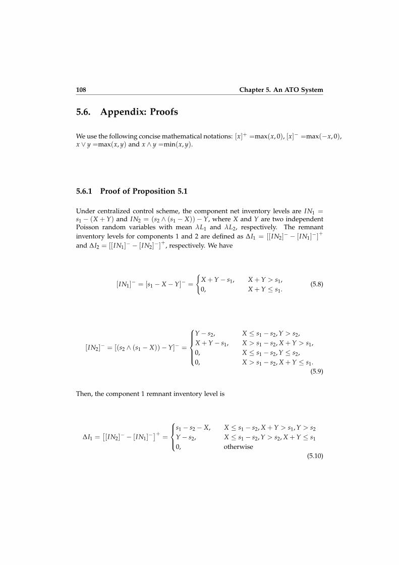
108 Chapter 5. An ATO System
5.6. Appendix: Proofs
We use the following concise mathematical notations: [x]+ =max(x, 0), [x]− =max(−x, 0),x ∨ y =max(x, y) and x ∧ y =min(x, y).
5.6.1 Proof of Proposition 5.1
Under centralized control scheme, the component net inventory levels are IN1 =s1 − (X + Y) and IN2 = (s2 ∧ (s1 − X))− Y, where X and Y are two independentPoisson random variables with mean λL1 and λL2, respectively. The remnantinventory levels for components 1 and 2 are defined as ∆I1 = [[IN2]
− − [IN1]−]
+
and ∆I2 = [[IN1]− − [IN2]
−]+, respectively. We have
[IN1]− = [s1 − X−Y]− =
{X + Y− s1, X + Y > s1,0, X + Y ≤ s1.
(5.8)
[IN2]− = [(s2 ∧ (s1 − X))−Y]− =
Y− s2, X ≤ s1 − s2, Y > s2,X + Y− s1, X > s1 − s2, X + Y > s1,0, X ≤ s1 − s2, Y ≤ s2,0, X > s1 − s2, X + Y ≤ s1.
(5.9)
Then, the component 1 remnant inventory level is
∆I1 =[[IN2]
− − [IN1]−]+ =
s1 − s2 − X, X ≤ s1 − s2, X + Y > s1, Y > s2
Y− s2, X ≤ s1 − s2, Y > s2, X + Y ≤ s1
0, otherwise(5.10)

5.6 Appendix: Proofs 109
Based on Equation (5.10), the expected component 1 remnant inventory level canbe calculated as
E{∆I1} =s1−s2
∑x=0
s1−x
∑y=s2+1
(y− s2)P2(y)P1(x) +s1−s2
∑x=0
∞
∑y=s1−x+1
(s1 − s2 − x)P2(y)P1(x)
=s1−s2
∑x=0
(s1−x
∑y=s2+1
(y− s2)P2(y) +∞
∑y=s1−x+1
(s1 − s2 − x)P2(y)
)P1(x)
=s1−s2
∑x=0
(s1−x
∑y=s2+1
(y− s2)P2(y) + (s1 − s2 − x)(1− F2(s1 − x))
)P1(x)
Similarly, using Equations (5.8) and (5.9), we get ∆I2 = [[IN1]− − [IN2]
−]+
= 0.Hence, the expected component 2 remnant inventory level is E{∆I2} = 0.
5.6.2 Simplification of Equation (5.2.4)
First, we rewrite Equation (5.2.4) using the aforementioned concise notations. Weobtain the following expression:
Ca(s, ψ) =h1
(E{[IN1]
+}+ E
{[[IN2]
− − [IN1]−]+})
+ h2
(E{[IN2]
+}+ E
{[[IN1]
− − [IN2]−]+})
+ pE{[IN1]
− ∨ [IN2]−}+ cλψ
By adding h1 (E {[IN1]−} −E {[IN1]
−}) and h2 (E {[IN2]−} −E {[IN2]
−}) to thefirst and second rows, respectively, we obtain
Ca(s, ψ) =h1
(E{[IN1]
+ − [IN1]−}+ E
{[[IN2]
− − [IN1]−]+ + [IN1]
−})
+ h2
(E{[IN2]
+ − [IN2]−}+ E
{[[IN1]
− − [IN2]−]+ + [IN2]
−})
+ pE{[IN1]
− ∨ [IN2]−}+ cλψ
For all x, y ∈ R, [x]+ − [x]− = x and [x− y]+ + y = x ∨ y (Szekli, 2012). Then thelast expression can be rewritten as follows:
Ca(s, ψ) =h1(E {IN1}+ E
{[IN1]
− ∨ [IN2]−})+ h2
(E {IN2}+ E
{[IN1]
− ∨ [IN2]−})
+ pE{[IN1]
− ∨ [IN2]−}+ cλψ
=h1E {IN1}+ h2E {IN2}+ (p + h1 + h2)E{[IN1]
− ∨ [IN2]−}+ cλψ
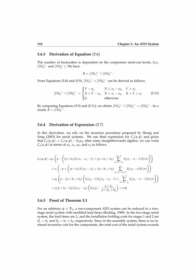
110 Chapter 5. An ATO System
5.6.3 Derivation of Equation (5.6)
The number of backorders is dependent on the component stock-out levels, (i.e.,[IN1]
− and [IN2]−). We have
B = [IN1]− ∨ [IN2]
−.
From Equations (5.8) and (5.9), [IN1]− ∨ [IN2]
− can be derived as follows:
[IN1]− ∨ [IN2]
− =
Y− s2, X ≤ s1 − s2, Y > s2
X + Y− s1, X > s1 − s2, X + Y > s1
0, otherwise(5.11)
By comparing Equations (5.9) and (5.11), we obtain [IN1]− ∨ [IN2]
− = [IN2]−. As a
result, B = [IN2]−.
5.6.4 Derivation of Expression (5.7)
In this derivation, we rely on the recursive procedure proposed by Shang andSong (2003) for serial systems. We use their expression for Cs(s, ψ) and giventhat Ca(s, ψ) = Cs(s, ψ)− h1µ2, after some straightforwards algebra, we can writeCa(s, ψ) in terms of µ1, s1, µ2, and s2 as follows.
Ca(s, ψ) =µ1
(p−
((p + h1)F1(s1 − s2 − 1) + (p + h1 + h2)
s1−1
∑n=s1−s2
F2(s1 − n− 1)P1(n)
))
+ s1
(−p +
((p + h1)F1(s1 − s2) + (p + h1 + h2)
s1
∑n=s1−s2+1
F2(s1 − n)P1(n)
))
+ µ2
(p− (p + h1 + h2)
(F2(s2 − 1)F1(s1 − s2 − 1) +
s1−1
∑n=s1−s2
F2(s1 − n− 1)P1(n)
))
+ s2(p + h1 + h2)F1(s1 − s2)
(F2(s2)−
p + h1p + h1 + h2
)+ cλψ
5.6.5 Proof of Theorem 5.1
For an arbitrary ψ ∈ Ψ1, a two-component ATO system can be reduced to a two-stage serial system with modified lead times (Rosling, 1989). In the two-stage serialsystem, the lead times are Lj and the installation holding costs for stages 1 and 2 areh′1 = h1 and h′2 = h1 + h2, respectively. Since in the assembly system, there is no in-transit inventory cost for the components, the total cost of the serial system exceeds
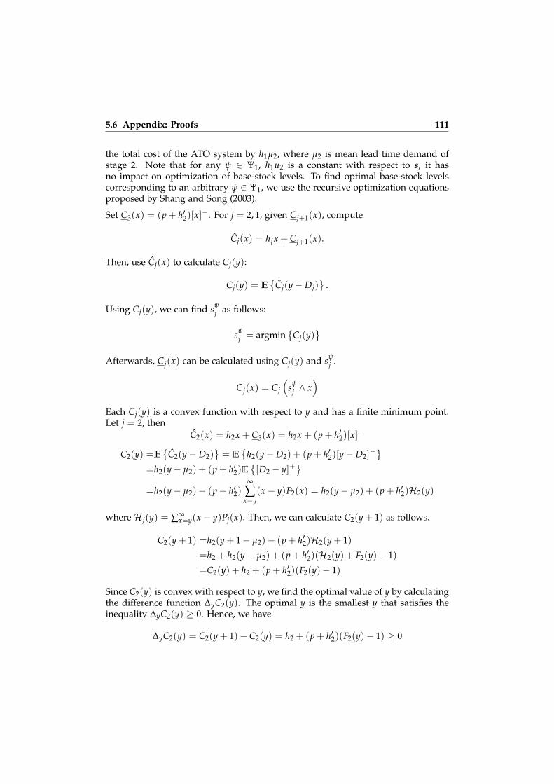
5.6 Appendix: Proofs 111
the total cost of the ATO system by h1µ2, where µ2 is mean lead time demand ofstage 2. Note that for any ψ ∈ Ψ1, h1µ2 is a constant with respect to s, it hasno impact on optimization of base-stock levels. To find optimal base-stock levelscorresponding to an arbitrary ψ ∈ Ψ1, we use the recursive optimization equationsproposed by Shang and Song (2003).
Set C3(x) = (p + h′2)[x]−. For j = 2, 1, given Cj+1(x), compute
Cj(x) = hjx + Cj+1(x).
Then, use Cj(x) to calculate Cj(y):
Cj(y) = E{
Cj(y− Dj)}
.
Using Cj(y), we can find sψj as follows:
sψj = argmin
{Cj(y)
}Afterwards, Cj(x) can be calculated using Cj(y) and sψ
j .
Cj(x) = Cj
(sψ
j ∧ x)
Each Cj(y) is a convex function with respect to y and has a finite minimum point.Let j = 2, then
C2(x) = h2x + C3(x) = h2x + (p + h′2)[x]−
C2(y) =E{
C2(y− D2)}= E
{h2(y− D2) + (p + h′2)[y− D2]
−}=h2(y− µ2) + (p + h′2)E
{[D2 − y]+
}=h2(y− µ2)− (p + h′2)
∞
∑x=y
(x− y)P2(x) = h2(y− µ2) + (p + h′2)H2(y)
where Hj(y) = ∑∞x=y(x− y)Pj(x). Then, we can calculate C2(y + 1) as follows.
C2(y + 1) =h2(y + 1− µ2)− (p + h′2)H2(y + 1)
=h2 + h2(y− µ2) + (p + h′2)(H2(y) + F2(y)− 1)
=C2(y) + h2 + (p + h′2)(F2(y)− 1)
Since C2(y) is convex with respect to y, we find the optimal value of y by calculatingthe difference function ∆yC2(y). The optimal y is the smallest y that satisfies theinequality ∆yC2(y) ≥ 0. Hence, we have
∆yC2(y) = C2(y + 1)− C2(y) = h2 + (p + h′2)(F2(y)− 1) ≥ 0

112 Chapter 5. An ATO System
The optimal y is the smallest non-negative integer number that satisfies
F2(y) ≥p + h′2 − h2
p + h′2=
p + h1
p + h1 + h2.
In other words,
sψ2 =
{y ∈N0 : F2(y− 1) <
p + h1
p + h1 + h2≤ F2(y)
}In addition, we have
C2(x) = C2(sψ2 ∧ x) = E
{C2
((sψ
2 ∧ x)− D2
)}= E
{h2
((sψ
2 ∧ x)− D2
)+ (p + h′2)
[(sψ
2 ∧ x)− D2
]−}= h2
((sψ
2 ∧ x)− µ2
)+ (p + h′2)E
{[D2 − (sψ
2 ∧ x)]+}
= h2
((sψ
2 ∧ x)− µ2
)+ (p + h′2)H2
(sψ
2 ∧ x)
We derive a similar expression for j = 1.
C1(x) = h1x + C2(x) = h1x + h2
((sψ
2 ∧ x)− µ2
)+ (p + h′2)H2
(sψ
2 ∧ x)
C1(y) =E{
C1(y− D1)}
=E{
h1(y− D1) + h2
((sψ
2 ∧ (y− D1))− µ2
)+ (p + h′2)H2(s
ψ2 ∧ (y− D1))
}=h1(y− µ1) + h2E
{(sψ
2 ∧ (y− D1))− µ2
}+ (p + h′2)E
{H2
(sψ
2 ∧ (y− D1))}
=h1(y− µ1) + h2
(sψ
2 −H1
(y− sψ
2 + 1)+ F1
(y− sψ
2
)− 1− µ2
)+ (p + h′2)
H2(sψ2 )F1
(y− sψ
2
)+
∞
∑n=y−sψ
2 +1
H2(y− n)P1(n)
Then, we have
C1(y + 1) =h1(y + 1− µ1) + h2
(sψ
2 −H1
(y + 1− sψ
2 + 1)+ F1
(y + 1− sψ
2
)− 1− µ2
)+ (p + h′2)
H2(sψ2 )F1
(y + 1− sψ
2
)+
∞
∑n=y+1−sψ
2 +1
H2(y + 1− n)P1(n)
=C1(y) + h1 + h2
(1− F1(y− sψ
2 ))
+ (p + h′2)
∞
∑n=y−sψ
2 +1
F2(y− n)P1(n)−(
1− F1(y− sψ2 ))
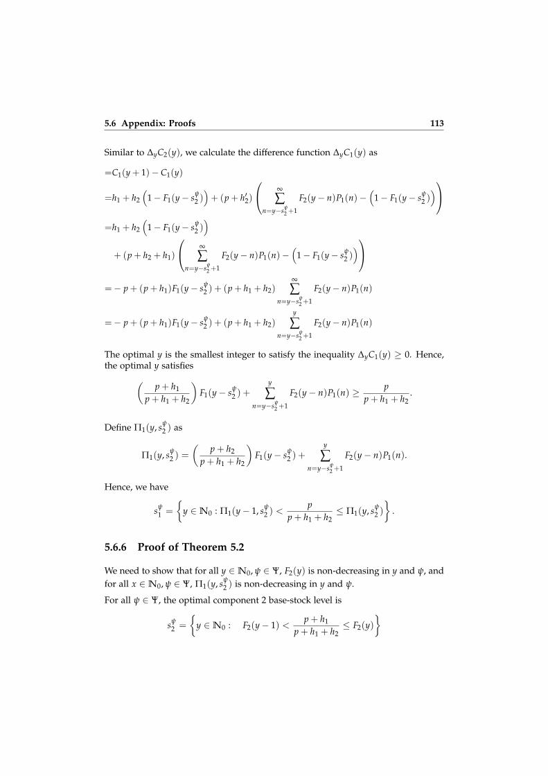
5.6 Appendix: Proofs 113
Similar to ∆yC2(y), we calculate the difference function ∆yC1(y) as
=C1(y + 1)− C1(y)
=h1 + h2
(1− F1(y− sψ
2 ))+ (p + h′2)
∞
∑n=y−sψ
2 +1
F2(y− n)P1(n)−(
1− F1(y− sψ2 ))
=h1 + h2
(1− F1(y− sψ
2 ))
+ (p + h2 + h1)
∞
∑n=y−sψ
2 +1
F2(y− n)P1(n)−(
1− F1(y− sψ2 ))
=− p + (p + h1)F1(y− sψ2 ) + (p + h1 + h2)
∞
∑n=y−sψ
2 +1
F2(y− n)P1(n)
=− p + (p + h1)F1(y− sψ2 ) + (p + h1 + h2)
y
∑n=y−sψ
2 +1
F2(y− n)P1(n)
The optimal y is the smallest integer to satisfy the inequality ∆yC1(y) ≥ 0. Hence,the optimal y satisfies(
p + h1
p + h1 + h2
)F1(y− sψ
2 ) +y
∑n=y−sψ
2 +1
F2(y− n)P1(n) ≥p
p + h1 + h2.
Define Π1(y, sψ2 ) as
Π1(y, sψ2 ) =
(p + h2
p + h1 + h2
)F1(y− sψ
2 ) +y
∑n=y−sψ
2 +1
F2(y− n)P1(n).
Hence, we have
sψ1 =
{y ∈N0 : Π1(y− 1, sψ
2 ) <p
p + h1 + h2≤ Π1(y, sψ
2 )
}.
5.6.6 Proof of Theorem 5.2
We need to show that for all y ∈N0, ψ ∈ Ψ, F2(y) is non-decreasing in y and ψ, andfor all x ∈N0, ψ ∈ Ψ, Π1(y, sψ
2 ) is non-decreasing in y and ψ.
For all ψ ∈ Ψ, the optimal component 2 base-stock level is
sψ2 =
{y ∈N0 : F2(y− 1) <
p + h1
p + h1 + h2≤ F2(y)
}

114 Chapter 5. An ATO System
Note that F2(y) is the cumulative distribution function of a Poisson random variablewith mean µ2 = λL2, where L2 = l2 − ψ depends on ψ. Hence, although F2(y)seems to be a function of y only, it is also a function of ψ by definition. In Chapter3, for a single location system we prove that F2(y) is non-decreasing in y and ψ.This result is sufficient to conclude that sψ
2 is non-increasing in ψ.
Next, we prove the result for sψ1 . We use the following lemma.
Lemma 5.2 Π1(y, sψ2 ) is non-decreasing in y and ψ for all y ∈N0, ψ ∈ Ψ.
Proof. We show that the first order difference function of Π1(y, sψ2 ) with respect to
y, defined as ∆yΠ1(y, sψ2 ), and the first derivative of Π1(y, sψ
2 ) with respect to ψ arenon-negative. We start with ∆yΠ1(y, sψ
2 ). For all ψ ∈ Ψ, we have
Π1(y + 1, sψ2 ) =
(p + h1
p + h1 + h2
)F1(y + 1− sψ
2 ) +y+1
∑n=y+1−sψ
2 +1
F2(y + 1− n)P1(n)
=
(p + h1
p + h1 + h2
)(F1(y− sψ
2 ) + P1(y− sψ2 + 1))
+y+1
∑n=y−sψ
2 +2
(F2(y− n) + P2(y− n + 1))P1(n)
=Π(y, sψ2 ) +
(p + h1
p + h1 + h2
)P1(y− sψ
2 + 1)− F2(sψ2 − 1)P1(y− sψ
2 + 1)
+y+1
∑n=y−sψ
2 +2
P2(y− n + 1)P1(n)
=Π(y, sψ2 ) + P1(y− sψ
2 + 1)(
h1 + pp + h1 + h2
− F2(sψ2 − 1)
)+
y+1
∑n=y−sψ
2 +2
P2(y− n + 1)P1(n)
Hence,
∆yΠ1(y, sψ2 ) = Π1(y + 1, sψ
2 )−Π1(y, sψ2 )
= P1(y− sψ2 + 1)
(h1 + p
p + h1 + h2− F2(s
ψ2 − 1)
)+
y+1
∑n=y−sψ
2 +2
P2(y− n + 1)P1(n).
For all sψ2 , we have F2(s
ψ2 − 1) < h1+p
p+h1+h2. Hence, ∆yΠ1(y, sψ
2 ) ≥ 0. Therefore, for all
ψ ∈ Ψ, Π1(y, sψ2 ) is non-decreasing in y.
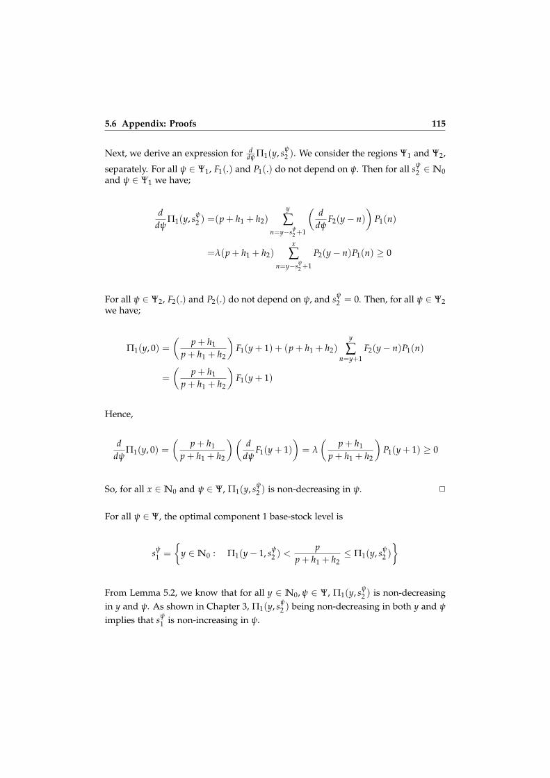
5.6 Appendix: Proofs 115
Next, we derive an expression for ddψ Π1(y, sψ
2 ). We consider the regions Ψ1 and Ψ2,
separately. For all ψ ∈ Ψ1, F1(.) and P1(.) do not depend on ψ. Then for all sψ2 ∈N0
and ψ ∈ Ψ1 we have;
ddψ
Π1(y, sψ2 ) =(p + h1 + h2)
y
∑n=y−sψ
2 +1
(d
dψF2(y− n)
)P1(n)
=λ(p + h1 + h2)x
∑n=y−sψ
2 +1
P2(y− n)P1(n) ≥ 0
For all ψ ∈ Ψ2, F2(.) and P2(.) do not depend on ψ, and sψ2 = 0. Then, for all ψ ∈ Ψ2
we have;
Π1(y, 0) =(
p + h1
p + h1 + h2
)F1(y + 1) + (p + h1 + h2)
y
∑n=y+1
F2(y− n)P1(n)
=
(p + h1
p + h1 + h2
)F1(y + 1)
Hence,
ddψ
Π1(y, 0) =(
p + h1
p + h1 + h2
)(d
dψF1(y + 1)
)= λ
(p + h1
p + h1 + h2
)P1(y + 1) ≥ 0
So, for all x ∈N0 and ψ ∈ Ψ, Π1(y, sψ2 ) is non-decreasing in ψ. 2
For all ψ ∈ Ψ, the optimal component 1 base-stock level is
sψ1 =
{y ∈N0 : Π1(y− 1, sψ
2 ) <p
p + h1 + h2≤ Π1(y, sψ
2 )
}
From Lemma 5.2, we know that for all y ∈ N0, ψ ∈ Ψ, Π1(y, sψ2 ) is non-decreasing
in y and ψ. As shown in Chapter 3, Π1(y, sψ2 ) being non-decreasing in both y and ψ
implies that sψ1 is non-increasing in ψ.

116 Chapter 5. An ATO System
5.6.7 Proof of Lemma 5.1
We show that (l1 − l2)c23 − l1c13 + l2c12 = 0. By replacing the value of thethresholds, ci j, based on their definition, then
(l1 − l2)
(Ca(sl2 , l2)− Ca(sl1 , l1)
λ(l1 − l2)+ c
)− l1
(Ca(s0, 0)− Ca(sl1 , l1)
λ(l1 − 0)+ c
)
+ l2
(Ca(s0, 0)− Ca(sl2 , l2)
λ(l2 − 0)+ c
)
=(l1 − l2)
(Ca(sl2 , l2)− Ca(sl1 , l1)
λ(l1 − l2)
)− l1
(Ca(s0, 0)− Ca(sl1 , l1)
λ(l1 − 0)
)
+ l2
(Ca(s0, 0)− Ca(sl2 , l2)
λ(l2 − 0)
)
=1λ(Ca(sl2 , l2)− Ca(sl1 , l1)− Ca(s0, 0) + Ca(sl1 , l1) + Ca(s0, 0)− Ca(sl2 , l2)) = 0
As a result, (l1 − l2)c23 − l1c13 + l2c12 = 0.
Next, we prove the second result. Suppose c23 ≥ c12 and define ε = c23 − c12 ≥ 0.Then, using (l1 − l2)c23 = l1c13 − l2c12, we obtain
c13 =
(1− l2
l1
)c23 +
l2l1
c12 =
(1− l2
l1
)(c12 + ε) +
l2l1
c12 = c12 +
(1− l2
l1
)ε
Since l2 ≤ l1 and ε ≥ 0, we have(
1− l2l1
)ε ≤ ε. Hence,
c13 = c12 +
(1− l2
l1
)ε ≤ c12 + ε = c23.
Considering this inequality with c12 ≤ c13, implies that c12 ≤ c13 ≤ c23.
Next, suppose c23 < c12 and define ε = c12 − c23 > 0. Then, using (l1 − l2)c23 =l1c13 − l2c12, we calculate c13 as follows:
c13 =
(1− l2
l1
)c23 +
l2l1
c12 =
(1− l2
l1
)(c12 − ε) +
l2l1
c12 = c12 +
(l2l1− 1)
ε
Since l2 < l1 and ε > 0, we have(
l2l1− 1)
ε > −ε. Hence,
c13 = c12 +
(l2l1− 1)
ε > c12 − ε = c23.
Considering this inequality with c12 > c13 implies that c23 < c13 < c12.
As a result, either c12 ≤ c13 ≤ c23 or c23 < c13 < c12 holds.
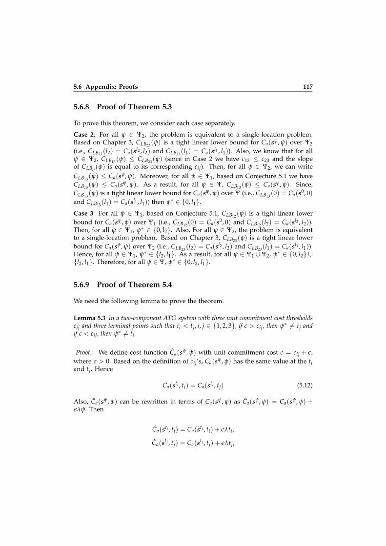
5.6 Appendix: Proofs 117
5.6.8 Proof of Theorem 5.3
To prove this theorem, we consider each case separately.
Case 2: For all ψ ∈ Ψ2, the problem is equivalent to a single-location problem.Based on Chapter 3, CLB23(ψ) is a tight linear lower bound for Ca(sψ, ψ) over Ψ2
(i.e., CLB23(l2) = Ca(sl2 , l2) and CLB23(l1) = Ca(sl1 , l1)). Also, we know that for allψ ∈ Ψ2, CLB13(ψ) ≤ CLB23(ψ) (since in Case 2 we have c13 ≤ c23 and the slopeof CLBij(ψ) is equal to its corresponding cij). Then, for all ψ ∈ Ψ2, we can writeCLB13(ψ) ≤ Ca(sψ, ψ). Moreover, for all ψ ∈ Ψ1, based on Conjecture 5.1 we haveCLB13(ψ) ≤ Ca(sψ, ψ). As a result, for all ψ ∈ Ψ, CLB13(ψ) ≤ Ca(sψ, ψ). Since,CLB13(ψ) is a tight linear lower bound for Ca(sψ, ψ) over Ψ (i.e., CLB13(0) = Ca(s0, 0)and CLB13(l1) = Ca(sl1 , l1)) then ψ∗ ∈ {0, l1}.Case 3: For all ψ ∈ Ψ1, based on Conjecture 5.1, CLB12(ψ) is a tight linear lowerbound for Ca(sψ, ψ) over Ψ1 (i.e., CLB12(0) = Ca(s0, 0) and CLB12(l2) = Ca(sl2 , l2)).Then, for all ψ ∈ Ψ1, ψ∗ ∈ {0, l2}. Also, For all ψ ∈ Ψ2, the problem is equivalentto a single-location problem. Based on Chapter 3, CLB23(ψ) is a tight linear lowerbound for Ca(sψ, ψ) over Ψ2 (i.e., CLB23(l2) = Ca(sl2 , l2) and CLB23(l1) = Ca(sl1 , l1)).Hence, for all ψ ∈ Ψ1, ψ∗ ∈ {l2, l1}. As a result, for all ψ ∈ Ψ1 ∪ Ψ2, ψ∗ ∈ {0, l2} ∪{l2, l1}. Therefore, for all ψ ∈ Ψ, ψ∗ ∈ {0, l2, l1}.
5.6.9 Proof of Theorem 5.4
We need the following lemma to prove the theorem.
Lemma 5.3 In a two-component ATO system with three unit commitment cost thresholdscij and three terminal points such that ti < tj, i, j ∈ {1, 2, 3}, if c > cij, then ψ∗ 6= tj andif c < cij, then ψ∗ 6= ti.
Proof. We define cost function Ca(sψ, ψ) with unit commitment cost c = cij + ε,where ε > 0. Based on the definition of cij’s, Ca(sψ, ψ) has the same value at the tiand tj. Hence
Ca(sti , ti) = Ca(stj , tj) (5.12)
Also, Ca(sψ, ψ) can be rewritten in terms of Ca(sψ, ψ) as Ca(sψ, ψ) = Ca(sψ, ψ) +ελψ. Then
Ca(sti , ti) = Ca(sti , ti) + ελti,
Ca(stj , tj) = Ca(stj , tj) + ελtj,
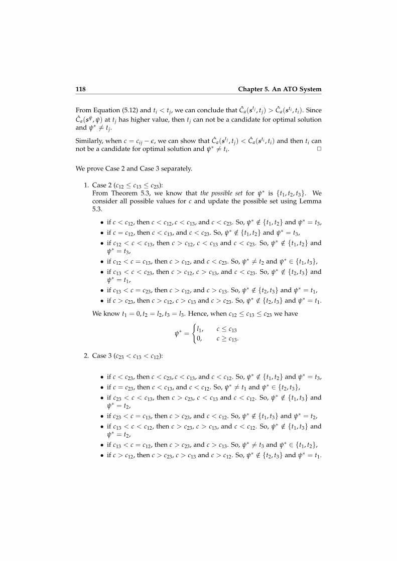
118 Chapter 5. An ATO System
From Equation (5.12) and ti < tj, we can conclude that Ca(stj , tj) > Ca(sti , ti). SinceCa(sψ, ψ) at tj has higher value, then tj can not be a candidate for optimal solutionand ψ∗ 6= tj.
Similarly, when c = cij − ε, we can show that Ca(stj , tj) < Ca(sti , ti) and then ti cannot be a candidate for optimal solution and ψ∗ 6= ti. 2
We prove Case 2 and Case 3 separately.
1. Case 2 (c12 ≤ c13 ≤ c23):From Theorem 5.3, we know that the possible set for ψ∗ is {t1, t2, t3}. Weconsider all possible values for c and update the possible set using Lemma5.3.
• if c < c12, then c < c12, c < c13, and c < c23. So, ψ∗ /∈ {t1, t2} and ψ∗ = t3,
• if c = c12, then c < c13, and c < c23. So, ψ∗ /∈ {t1, t2} and ψ∗ = t3,
• if c12 < c < c13, then c > c12, c < c13 and c < c23. So, ψ∗ /∈ {t1, t2} andψ∗ = t3,
• if c12 < c = c13, then c > c12, and c < c23. So, ψ∗ 6= t2 and ψ∗ ∈ {t1, t3},• if c13 < c < c23, then c > c12, c > c13, and c < c23. So, ψ∗ /∈ {t2, t3} and
ψ∗ = t1,
• if c13 < c = c23, then c > c12, and c > c13. So, ψ∗ /∈ {t2, t3} and ψ∗ = t1,
• if c > c23, then c > c12, c > c13 and c > c23. So, ψ∗ /∈ {t2, t3} and ψ∗ = t1.
We know t1 = 0, t2 = l2, t3 = l3. Hence, when c12 ≤ c13 ≤ c23 we have
ψ∗ =
{l1, c ≤ c13
0, c ≥ c13.
2. Case 3 (c23 < c13 < c12):
• if c < c23, then c < c23, c < c13, and c < c12. So, ψ∗ /∈ {t1, t2} and ψ∗ = t3,
• if c = c23, then c < c13, and c < c12. So, ψ∗ 6= t1 and ψ∗ ∈ {t2, t3},• if c23 < c < c13, then c > c23, c < c13 and c < c12. So, ψ∗ /∈ {t1, t3} and
ψ∗ = t2,
• if c23 < c = c13, then c > c23, and c < c12. So, ψ∗ /∈ {t1, t3} and ψ∗ = t2,
• if c13 < c < c12, then c > c23, c > c13, and c < c12. So, ψ∗ /∈ {t1, t3} andψ∗ = t2,
• if c13 < c = c12, then c > c23, and c > c13. So, ψ∗ 6= t3 and ψ∗ ∈ {t1, t2},• if c > c12, then c > c23, c > c13 and c > c12. So, ψ∗ /∈ {t2, t3} and ψ∗ = t1.

5.6 Appendix: Proofs 119
We know t1 = 0, t2 = l2, t3 = l3. Hence, when c23 < c13 < c12 we have
ψ∗ =
l1, c ≤ c23
l2, c23 ≤ c ≤ c12
0, c ≥ c12.


6Conclusions
In this thesis, we examined the preorder strategy in the context of inventoryand service management. Under the preorder strategy, customers place theirorders ahead of their actual need based on a pre-determined time window calledcommitment lead time and, in turn, they receive a bonus based on the length ofthe commitment lead time, which is a called commitment cost from the systemmanager’s perspective. To investigate the impact of the commitment lead time onthe replenishment policy and customer service, we considered inventory systemswith different settings. These inventory systems face Poisson customer demand andreplenish their inventory based on continuous base-stock policies with deterministicreplenishment lead times. Also, unmet demands are backorered. The systemsmanagers’ objective is to find the optimal control policy as a combination of thebase-stock levels and commitment lead time such that the long-run average totalcost is minimized. Since the base-stock levels are discrete and the commitmentlead time is continuous, we were dealing with Mixed-integer, Nonlinear Programs(MINLP). In an inventory system with commitment lead time, customer providethe ADI to the system. In this case, the inventory position of the system dependson the known demand. This leads to the nice result that we can just subtract thecommitment lead time from the replenishment lead time.
With the above-mentioned settings, in Chapter 3, we studied a single-location in-ventory system with preorder strategy. By replacing backordering cost with a time-based service constraint, a single-location inventory system with preorder strategyand service constraint was formed and analyzed in Chapter 4. Furthermore, a morecomplex inventory system with ATO structure and preorder strategy was analyzedin Chapter 5.
In the following, we first reiterate the main findings of this thesis, and then, we

122 Chapter 6. Conclusions
provide some possible extensions of the commitment lead time that can contributeto the literature of inventory and service management.
6.1. Results and Findings
In Chapter 2, a comprehensive review of the recent literature on inventorymanagement with ADI was provided. In this chapter, we identified the researchgaps and represented the exposition of our research within the body of existingliterature.
In Chapter 3, we studied a single-location inventory system with commitment leadtime. We aimed to find the optimal control policy such that the long-run averagetotal cost consisting of holding, backordering, and commitment costs is minimized.We proved the convexity of the cost function in each decision variable. We showedthat the optimal base-stock level is non-increasing in the length of the commitmentlead time. The long-run average cost as a function of a commitment lead timeand the corresponding optimal base-stock level served as a continuous piecewise-convex lower bound on the original average cost function. We constructed anothermonotone lower bound on this piecewise-convex lower bound. This monotonelower bound implied the optimality of the bang-bang policy for the commitmentlead time. Under this policy, the commitment lead time is either zero or themaximum possible value, which is the replenishment lead time. In addition,we showed that the corresponding optimal base-stock policy is of all-or-nothingtype. Hence, the optimal base-stock level is either zero or the solution of the well-known Newsvendor problem with zero commitment lead time. The optimalityof the bang-bang policy holds for general commitment cost structures under avery mild condition. As a specific case, we studied a linear commitment cost.For this case, we found a unit commitment cost threshold which dictates theoptimality of either a buy-to-order (BTO) or a buy-to-stock (BTS) strategy. Morespecifically, we showed that when the unit commitment cost is less than the unitcommitment cost threshold, the optimal ordering strategy is BTO strategy (i.e.,the optimal commitment lead time is equal to replenishment lead time and theoptimal base-stock level is zero) and when the unit commitment cost is more thanthe unit commitment cost threshold, the optimal strategy is a BTS strategy (i.e., theoptimal commitment lead time is zero and optimal base-stock level is non-zero).Moreover, we showed that the unit commitment cost threshold is increasing in theunit holding and backordering costs and decreasing in the mean lead time demand.For a given base-stock level, we developed a simple and accurate approximationfor the corresponding optimal commitment lead time. Finally, we determined theconditions on the unit commitment cost for the profitability of the BTO strategy (seeFigure 6.1).

6.1 Results and Findings 123
Unit commitment cost threshold
BTS
BTO
BTO
Profitable
Non-profitable
Mean lead time demand
Uni
tco
mm
itm
ent
cost
Figure 6.1: Optimal strategies
In Chapter 4, we extend our problem in Chapter 3 by replacing the backorderingcost term with a time-based service constraint. The firm manager aims to find theoptimal control policy such that a long-run average total cost consisting of holdingand commitment costs is minimized subject to a time-based service constraint.We studied this problem with two time-based service measures; average customerwaiting time and individual customer waiting time. For the first measure, we puta maximum waiting threshold on the average customer waiting time (see Figure6.2). For the second, we formed a chance constraint consisting of a service levelas well as the maximum waiting threshold. Since we deal with two constraint,mixed-integer, nonlinear programs (C-MINP), finding closed-form solutions are notpossible. Instead, we proposed exact and heuristic optimization algorithms for eachoptimization model. Using a comprehensive numerical experiment we showed thatthe heuristic algorithms performs quite well.
tt t
Agreed delivery(on-time fulfillment)
Actual delivery
Commitment lead time Customer waiting time
Time
Replenishment lead time∞
Customer order
Firm321
Max. waiting threshold
ω
t +ω2
Figure 6.2: An illustration of the commitment lead time and customer waiting time
We observed that when commitment lead time and time-based service measureswith positive maximum waiting threshold are taken into account, the optimalcommitment lead time is not a bang-bang policy, anymore. However, for β−servicelevel type (i.e., the chance constraint with zero maximum waiting threshold), theoptimal commitment lead time takes a bang-bang form, under which the optimalcommitment lead time is either zero or l + lnβ
λ . We derived the exact distributionprobability of customer waiting time in terms of system parameters and controlpolicy. We showed that the commitment lead time not only increases the servicelevel but also decreases the possible maximum waiting time. We found that the

124 Chapter 6. Conclusions
commitment lead time plays a significant role in the determination of the optimalcontrol policy when either the maximum waiting threshold is small enough (e.g.,close to zero) or the service level is high enough (e.g., close to one). In otherwords, when the firm wants to provide a quicker response to a higher percentageof the customers, the value of commitment lead time in terms of cost reduction ismore highlighted. We showed that for any arbitrary maximum waiting threshold,the optimal cost value is bounded and non-increasing in the maximum waitingthreshold. Moreover, we considered an unconstraint optimization model withbackordering cost and its equivalent constraint optimization model with the averagewaiting time constraint. We calculated equivalent unit backordering cost such thatboth models have the same optimal cost. We found a negative relationship betweenunit backordering cost and maximum waiting threshold. When commitment leadtime is taken into account, the equivalent unit backordering cost is always boundedabove.
In Chapter 5, we considered a manufacturer who operates a two-component, single-end-product ATO system under preorder strategy and centralized control scheme.The manufacturer uses base-stock policies to replenish components inventories.The manufacturer aims to find the optimal component base-stock levels and theoptimal commitment lead time such that the long-run average total cost consistingof component inventory holding cost, backordering cost and commitment cost isminimized. For an arbitrary commitment lead time, we determined the optimalbase-stock levels by optimizing two nested convex functions recursively. We foundthat the optimal base-stocks are piecewise constant and non-increasing in thecommitment lead time. We defined three unit commitment cost thresholds, cij.Based on the order of these thresholds, we proved that we face either Case 2 orCase 3 (see Figure 6.3 for the order of the thresholds associated with each case).
0 c12 c23c13c
Component 1
Component 2
BTO BTS
BTO BTS
(a) Case 2
0 c23 c12c13c
Component 1
Component 2
BTO BTS
BTO BTS
(b) Case 3
Figure 6.3: Optimal strategies for the components in terms of the unit commitment cost
These thresholds enable the manufacturer to evaluate the benefit of the preorderstrategy under different unit commitment costs. We characterized the structure ofthe optimal preorder strategy and showed that the optimal commitment lead timeis either zero or equal to one of the components lead times. When the optimalcommitment lead time is zero, the preorder strategy is not beneficial. Hence, themanufacturer should choose a BTS strategy. When the optimal commitment leadtime equals the lead time of the component with the shorter lead time, the optimal

6.2 Further Research 125
strategy for this component is BTO and it is BTS for the other component. Onthe other hand, if the optimal commitment lead time equals the lead time of thecomponent with the longer lead time, the optimal strategy is the BTO strategy forboth components. We determined the conditions, under which one of these threecases holds.
6.2. Further Research
The framework developed in this thesis allows us to understand the role ofcommitment lead time in enhancing performance (i.e, operational costs reduction)and profitability of the inventory systems in different settings. Although weinvestigated the impact of commitment lead time in basic inventory systemsstructures, our analysis can be used as a building block to compose more complexsupply chain structures. For instance, providing a rigorous proof for a single-location inventory system with compound Poisson can serve as an interestingextension to what we have carried out for the single-location inventory system withpure Poisson customer demand.
Another interesting case for future research can be a multi-component, multi-end-product ATO system, in which each end-product has a dedicated commitmentlead time. In such a system, studying the impact of the commitment lead timeson the system performance and profitability will help the system manager toimprove the cost efficiency and responsiveness of the system, simultaneously. Itis worth mentioning that each of the above-mentioned extensions adds sufficientcomplexity and makes the problem less tractable. For instance, considering adedicated commitment lead time for each end-product increases the dimension ofthe problem in terms of decision variables. Since optimal control policies for generalmulti-component, multi-end-product ATO systems are unknown, finding heuristicpolicies will be a notable achievement.
Considering supply uncertainty in the form of supply disruptions (see Atan andSnyder (2012b), Atan and Snyder (2012a), Atan and Rousseau (2016), and Atan andSnyder (2014)) with commitment lead time can be another possible extension of thisresearch. It would be interesting to see how this form of supply uncertainty affectsthe optimal preordering strategy.

Bibliography
T. Ahmadi, Z. Atan, I. Adan, and T. de Kok. Optimal control policies for aninventory system with commitment lead time. Naval Research Logistics (NRL),2019a.
T. Ahmadi, Z. Atan, T. de Kok, and I. Adan. Optimal control policies for assemble-to-order systems with commitment lead time. IISE Transactions, 2019b.
K. Altendorfer and S. Minner. Simultaneous optimization of capacity and plannedlead time in a two-stage production system with different customer due dates.European Journal of Operational Research, 213(1):134–146, 2011.
K. Altendorfer and S. Minner. A comparison of make-to-stock and make-to-order inmulti-product manufacturing systems with variable due dates. IIE Transactions,46(3):197–212, 2014.
A. Angelus and O. Ozer. Knowledge you can act on: optimal policies for assemblysystems with expediting and advance demand information. Operations Research,64(6):1338–1371, 2016.
Z. Atan and M. Rousseau. Inventory optimization for perishables subject to supplydisruptions. Optimization Letters, 10(1):89–108, 2016.
Z. Atan and L. V. Snyder. Disruptions in one-warehouse multiple-retailer systems.2012a.
Z. Atan and L. V. Snyder. Inventory strategies to manage supply disruptions. InSupply Chain Disruptions, pages 115–139. Springer, 2012b.
Z. Atan and L. V. Snyder. EOQ models with supply disruptions. In Handbook ofEOQ inventory problems, pages 43–55. Springer, 2014.
Z. Atan, T. Ahmadi, C. Stegehuis, T. de Kok, and I. Adan. Assemble-to-ordersystems: A review. European Journal of Operational Research, 261(3):866–879, 2017.
S. Axsater. Inventory control. Springer, 2006.
M. H. Benbitour and E. Sahin. Evaluation of the impact of uncertain advancedemand information on production/inventory systems. In 15th IFAC Symposiumon Information Control Problems in Manufacturing, 2015.

128 Bibliography
S. Benjaafar and M. ElHafsi. Production and inventory control of a single productassemble-to-order system with multiple customer classes. Management Science, 52(12):1896–1912, 2006.
S. Benjaafar, W. L. Cooper, and S. Mardan. Production-inventory systems withimperfect advance demand information and updating. Naval Research Logistics(NRL), 58(2):88–106, 2011.
F. Bernstein and G. A. DeCroix. Advance demand information in a multiproductsystem. Manufacturing & Service Operations Management, 17(1):52–65, 2014.
K. E. Bourland, S. G. Powell, D. F. Pyke, et al. Exploiting timely demand informationto reduce inventories. European Journal of Operational Research, 92(2):239–253, 1996.
J. A. Buzacott and J. Shanthikumar. Safety stock versus safety time in mrp controlledproduction systems. Management Science, 40(12):1678–1689, 1994.
K. D. Cattani and G. C. Souza. Inventory rationing and shipment flexibilityalternatives for direct market firms. Production and Operations Management, 11(4):441–457, 2002.
F. Chen. Market segmentation, advanced demand information, and supply chainperformance. Manufacturing & Service Operations Management, 3(1):53–67, 2001.
F. Chen and Y.-S. Zheng. Lower bounds for multi-echelon stochastic inventorysystems. Management Science, 40(11):1426–1443, 1994.
P. Chintapalli, S. M. Disney, and C. S. Tang. Coordinating supply chains viaadvance-order discounts, minimum order quantities, and delegations. Productionand Operations Management, 26(12):2175–2186, 2017.
D. Claudio and A. Krishnamurthy. Kanban-based pull systems with advancedemand information. International Journal of Production Research, 47(12):3139–3160,2009.
T. de Kok. Backorder lead time behaviour in (s, Q)-inventory models withcompound renewal demand. 1993.
T. de Kok. Evaluation and optimization of strongly ideal assemble-to-order systems.In Stochastic modeling and optimization of manufacturing systems and supply chains,pages 203–242. Springer, 2003.
M. K. Dogru, T. de Kok, and G.-J. van Houtum. A numerical study on the effectof the balance assumption in one-warehouse multi-retailer inventory systems.Flexible Services and Manufacturing Journal, 21(3-4):114–147, 2009.
G. J. Feeney and C. C. Sherbrooke. The (s - 1, s) inventory policy under compoundpoisson demand. Management Science, 12(5):391–411, 1966.
G. Gallego and O. Ozer. Integrating replenishment decisions with advance demandinformation. Management Science, 47(10):1344–1360, 2001.
Bibliography 129
G. Gallego and O. Ozer. Optimal replenishment policies for multiechelon inventoryproblems under advance demand information. Manufacturing & Service OperationsManagement, 5(2):157–175, 2003.
J.-P. Gayon, S. Benjaafar, and F. De Vericourt. Using imperfect advance demandinformation in production-inventory systems with multiple customer classes.Manufacturing & Service Operations Management, 11(1):128–143, 2009.
S. M. Gilbert and R. H. Ballou. Supply chain benefits from advanced customercommitments. Journal of Operations Management, 18(1):61–73, 1999.
A. Y. Ha, S. Tong, and H. Zhang. Sharing demand information in competing supplychains with production diseconomies. Management Science, 57(3):566–581, 2011.
R. Hariharan and P. Zipkin. Customer-order information, leadtimes, andinventories. Management Science, 41(10):1599–1607, 1995.
X. Hu, I. Duenyas, and R. Kapuscinski. Advance demand information and safetycapacity as a hedge against demand and capacity uncertainty. Manufacturing &Service Operations Management, 5(1):55–58, 2003.
T. Huang and J. A. van Mieghem. Clickstream data and inventory management:Model and empirical analysis. Production and Operations Management, 23(3):333–347, 2014.
T. Iida and P. Zipkin. Competition and cooperation in a two-stage supply chainwith demand forecasts. Operations Research, 58(5):1350–1363, 2010.
S. M. Iravani, T. Liu, K. Luangkesorn, and D. Simchi-Levi. A produce-to-stocksystem with advance demand information and secondary customers. NavalResearch Logistics (NRL), 54(3):331–345, 2007.
A. V. Iyer, V. Deshpande, and Z. Wu. A postponement model for demandmanagement. Management Science, 49(8):983–1002, 2003.
F. Karaesmen, G. Liberopoulos, and Y. Dallery. The value of advance demandinformation in production/inventory systems. Annals of Operations Research, 126(1-4):135–157, 2004.
G. Kiesmuller and T. de Kok. The customer waiting time in an (R, s, Q) inventorysystem. International Journal of Production Economics, 104(2):354–364, 2006.
Y. L. Kocaga and A. Sen. Spare parts inventory management with demand leadtimes and rationing. IIE Transactions, 39(9):879–898, 2007.
W. K. Kruse. Waiting time in an (s- 1, s) inventory system with arbitrarily distributedlead times. Operations Research, 28(2):348–352, 1980.
H. L. Lee, K. C. So, and C. S. Tang. The value of information sharing in a two-levelsupply chain. Management Science, 46(5):626–643, 2000.
130 Bibliography
G. Liberopoulos. On the tradeoff between optimal order-base-stock levels anddemand lead-times. European Journal of Operational Research, 190(1):136–155, 2008.
G. Liberopoulos and S. Koukoumialos. Tradeoffs between base stock levels,numbers of kanbans, and planned supply lead times in production/inventorysystems with advance demand information. International Journal of ProductionEconomics, 96(2):213–232, 2005.
G. Liberopoulos and S. Koukoumialos. On the effect of variability and uncertaintyin advance demand information on the performance of a make-to-stock supplier.MIBES Transactions International Journal, 2(1):95–114, 2008.
Y. Lu, J.-S. Song, and D. D. Yao. Order fill rate, leadtime variability, and advancedemand information in an assemble-to-order system. Operations Research, 51(2):292–308, 2003.
H. Lutze and O. Ozer. Promised lead-time contracts under asymmetric information.Operations Research, 56(4):898–915, 2008.
K. McCardle, K. Rajaram, and C. S. Tang. Advance booking discount programsunder retail competition. Management Science, 50(5):701–708, 2004.
K. Nakade and S. Yokozawa. Optimization of two-stage production/inventorysystems under order base stock policy with advance demand information. Journalof Industrial Engineering International, 12(4):437–458, 2016.
O. Ozer. Replenishment strategies for distribution systems under advance demandinformation. Management Science, 49(3):255–272, 2003.
O. Ozer and W. Wei. Inventory control with limited capacity and advance demandinformation. Operations Research, 52(6):988–1000, 2004.
F. Papier. Supply allocation under sequential advance demand information.Operations Research, 64(2):341–361, 2016.
F. Papier and U. W. Thonemann. Capacity rationing in stochastic rental systemswith advance demand information. Operations Research, 58(2):274–288, 2010.
K. Rosling. Optimal inventory policies for assembly systems under randomdemands. Operations Research, 37(4):565–579, 1989.
K. H. Shang and J.-S. Song. Newsvendor bounds and heuristic for optimal policiesin serial supply chains. Management Science, 49(5):618–638, 2003.
W. Shang and L. Liu. Promised delivery time and capacity games in time-basedcompetition. Management Science, 57(3):599–610, 2011.
E. A. Silver, D. F. Pyke, and D. J. Thomas. Inventory and production management insupply chains. CRC Press, 2016.
J.-S. Song. On the order fill rate in a multi-item, base-stock inventory system.
Bibliography 131
Operations Research, 46(6):831–845, 1998.
H. Stadtler and C. Kilger. Supply chain management and advanced planning.Concepts, Models, Software and Case Studies, 4:53–54, 2008.
R. Szekli. Stochastic ordering and dependence in applied probability, volume 97. SpringerScience & Business Media, 2012.
T. Tan, R. Gullu, and N. Erkip. Modelling imperfect advance demand informationand analysis of optimal inventory policies. European Journal of Operational Research,177(2):897–923, 2007.
T. Tan, R. Gullu, and N. Erkip. Using imperfect advance demand information inordering and rationing decisions. International Journal of Production Economics, 121(2):665–677, 2009.
H. Tempelmeier and L. Fischer. Approximation of the probability distribution ofthe customer waiting time under an (R,s,Q) inventory policy in discrete time.International Journal of Production Research, 48(21):6275–6291, 2010.
E. Topan, T. Tan, G.-J. van Houtum, and R. Dekker. Using imperfect advancedemand information in lost-sales inventory systems with the option of returninginventory. IISE Transactions, 50(3):246–264, 2018.
M. C. van der Heijden and T. de Kok. Customer waiting times in an (R, S) inventorysystem with compound poisson demand. Zeitschrift fur Operations Research, 36(4):315–332, 1992.
K. van Donselaar, L. R. Kopczak, and M. Wouters. The use of advance demandinformation in a project-based supply chain. European Journal of OperationalResearch, 130(3):519–538, 2001.
G.-J. van Houtum and B. Kranenburg. Spare parts inventory control under systemavailability constraints, volume 227. Springer, 2015.
G.-J. van Houtum and W. H. Zijm. On the relationship between cost and servicemodels for general inventory systems. Statistica Neerlandica, 54(2):127–147, 2000.
J. Wijngaard and F. Karaesmen. Advance demand information and a restrictedproduction capacity: on the optimality of order base-stock policies. OR Spectrum,29(4):643–660, 2007.
F. Zhang. Competition, cooperation, and information sharing in a two-echelonassembly system. Manufacturing & Service Operations Management, 8(3):273–291,2006.
K. Zhu and U. W. Thonemann. Modeling the benefits of sharing future demandinformation. Operations Research, 52(1):136–147, 2004.
P. Zipkin. Foundations of inventory management. McGraw Hill, Boston, Massachusetts,2000.

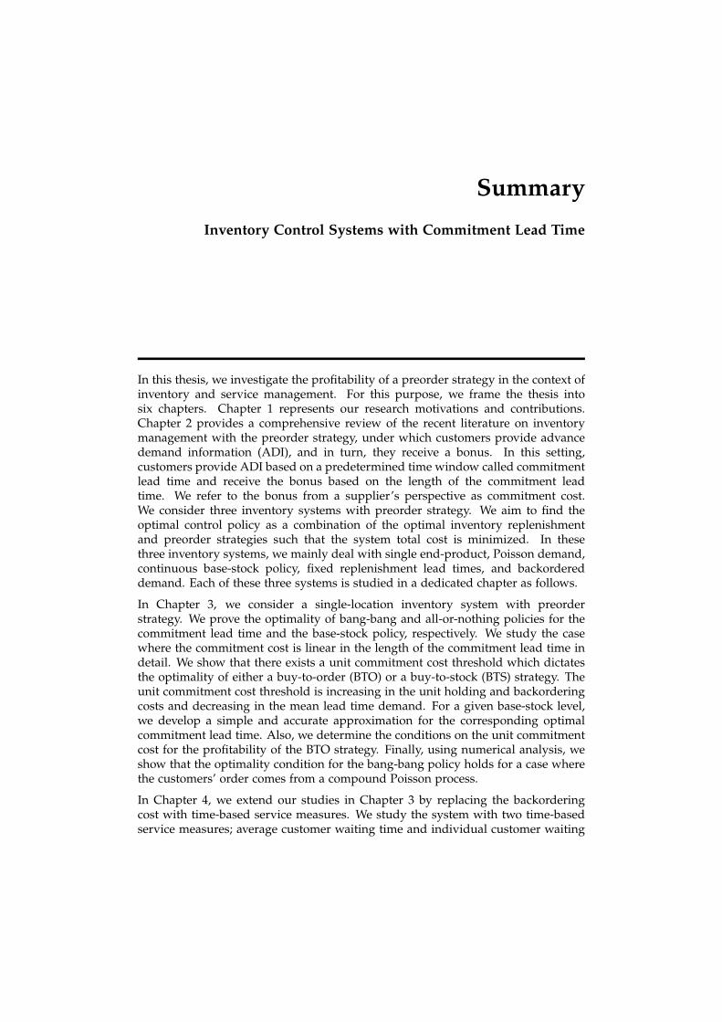
Summary
Inventory Control Systems with Commitment Lead Time
In this thesis, we investigate the profitability of a preorder strategy in the context ofinventory and service management. For this purpose, we frame the thesis intosix chapters. Chapter 1 represents our research motivations and contributions.Chapter 2 provides a comprehensive review of the recent literature on inventorymanagement with the preorder strategy, under which customers provide advancedemand information (ADI), and in turn, they receive a bonus. In this setting,customers provide ADI based on a predetermined time window called commitmentlead time and receive the bonus based on the length of the commitment leadtime. We refer to the bonus from a supplier’s perspective as commitment cost.We consider three inventory systems with preorder strategy. We aim to find theoptimal control policy as a combination of the optimal inventory replenishmentand preorder strategies such that the system total cost is minimized. In thesethree inventory systems, we mainly deal with single end-product, Poisson demand,continuous base-stock policy, fixed replenishment lead times, and backordereddemand. Each of these three systems is studied in a dedicated chapter as follows.
In Chapter 3, we consider a single-location inventory system with preorderstrategy. We prove the optimality of bang-bang and all-or-nothing policies for thecommitment lead time and the base-stock policy, respectively. We study the casewhere the commitment cost is linear in the length of the commitment lead time indetail. We show that there exists a unit commitment cost threshold which dictatesthe optimality of either a buy-to-order (BTO) or a buy-to-stock (BTS) strategy. Theunit commitment cost threshold is increasing in the unit holding and backorderingcosts and decreasing in the mean lead time demand. For a given base-stock level,we develop a simple and accurate approximation for the corresponding optimalcommitment lead time. Also, we determine the conditions on the unit commitmentcost for the profitability of the BTO strategy. Finally, using numerical analysis, weshow that the optimality condition for the bang-bang policy holds for a case wherethe customers’ order comes from a compound Poisson process.
In Chapter 4, we extend our studies in Chapter 3 by replacing the backorderingcost with time-based service measures. We study the system with two time-basedservice measures; average customer waiting time and individual customer waiting
134 Summary
time. For the former, we put a maximum waiting threshold on the average customerwaiting time. For the latter, we form a chance constraint consisting of a service levelas well as the maximum waiting threshold. Since finding closed-form solutionsare not possible, we propose exact and heuristic optimization algorithms for eachoptimization model. We observe that when commitment lead time and time-based service measures with positive maximum waiting threshold are considered,the optimal commitment lead time is not always a bang-bang policy. We derivethe exact distribution probability of customer waiting time in terms of systemparameters and control policy. We show that the commitment lead time not onlyincreases the service level but also decreases the possible maximum waiting time.Also, the commitment lead time provides optimal cost values bounded above forany service level and maximum waiting threshold. We find that when the firmwants to provide a quicker response to a higher percentage of the customers, thevalue of commitment lead time in terms of cost reduction is more highlighted.
In Chapter 5, we consider a two-component, single-end product ATO system withpreorder strategy. We find that the optimal commitment lead time is either zeroor equals to the replenishment lead time of one of the components. When theoptimal commitment lead time is zero, the preorder strategy is not beneficial andthe optimal control strategy for both components is the BTS strategy. When theoptimal commitment lead time is equal to the replenishment lead time of thecomponent with the shorter replenishment lead time, the optimal control strategyfor this component is BTO and it is BTS for the other component. On the otherhand, when the optimal commitment lead time is equal to the replenishment leadtime of the component with the longer replenishment lead time, the optimal controlstrategy is the BTO strategy for both components. We find the unit commitmentcost thresholds which determine the conditions under which one of these threecases holds.
Conclusions are drawn in Chapter 6. The main aim of the thesis has been reached.The authors suggest that the commitment lead time concept can be applied to moregeneral ATO systems with multiple end-products in which each end-product hasa dedicated commitment lead time. Although the complexity of the system isincreased, it can provide a considerable improvement in terms of responsivenessand product diversification of the system.

About the author
Taher Ahmadi was born in Mahabad, Iran in 1986. He finished his pre-collegeeducation in Mathematics and Physics. In 2009, he started his bachelor’s studies inIndustrial Engineering and graduated as the first best student of Isfahan Universityof Technology, Isfahan, Iran. He continued his studies at Tehran PolytechnicUniversity and obtained his master’s degree in Industrial Engineering in 2011.He worked at an automobile manufacturer, Parskhodro Co., in Tehran from 2010to 2014 as an Industrial Engineer. In October 2014, he joined OPAC group atEindhoven University of Technology (TU/e) to conduct his Ph.D. research underthe supervision of Prof. Ton de Kok, Prof. Ivo Adan, and Dr. Zumbul Atan.He also visited McCombs School of Business at the University of Texas at Austinfor three months to collaborate with Prof. Kumar Muthuraman. In August 2018,Taher joined a pharmaceutical company, Amgen Inc., in Breda as an OperationalExcellence project manager.