Invariant Theoryand

Differential Equations

Peter J. OlvertSchool of MathematicsUniversity of MinnesotaMinneapolis, MNUSA 55455

In: Invariant Theory, S.S. Koh, ed., Lecture Notes in Math, vol. 1278,Springer-Verlag, New York, 1987, pp. 62-80.

t Research Supported in Part by NSFGrant DMS 86-02004.

1. Introduction

Recent years have witnessed a resurgence of interest in classical invariant theory.

In the field of differential equations, it has become of steadily increasing importance, not

only in the applications to be discussed here, but also in the theory of canonical forms of

Hamiltonian systems, [4], and the study of conservation laws, [20]. The present work

originally arose in the study of nonconvex variational problems of interest in elasticity for

which one could prove existence of weak minimizers. A transform introduced by Gel'fand

and Dikii, [7], and Shakiban, [19], changes this problem into one about the primality of

certain determinantal ideals, and thus provides a complete solution. Subsequently the

transform method has been applied to a wide range of problems arising in the study of

differential equations and the calculus of variations. It has also been recognized, [14], that

when the functions are homogeneous polynomials, the transform method is equivalent to

the classical symbolic method of invariant theory. This paper will review the transform

method, its relationship and application to classical invariant theory, and its application to

problems arising in the calculus of variations. The last section provides a brief summary of

a new, and potentially important theory of higher order differential forms ("hyperforms")

which has arisen in an attempt to understand new divergence identities for transvectants

which are a direct result of these investigations.

Throughout, we will let x = (x1,...,*1*) be the independent variables and u =(u ,...,uq) be the dependent variables in somesystem of differential equations, so that theu's are to be viewed as functions of the x's. Partial derivatives will be denoted by

subscripts, e.g. u12=3 u/dx 9x , ormore generally using multi-index notation, so u" for

I=(i|,...,ifc) will denote the k-th order partial derivative 3kua/3x l...dxk. Adifferentialpolynomial is a complex-valued polynomial in the derivatives xxf (for simplicity we areexcluding explicit x dependence in our differential polynomials). A differential

polynomial is called differentially homogeneous of order k if it depends exclusively on

derivatives of order k; algebraically homogeneous refers to the usual concept ofhomogeneity for polynomials. Thus ^\\^2T"U\2 is differentially homogeneous of degree2, but not algebraically homogeneous, whereas ^i^l^^l^W *s algebraicallyhomogeneous of degree 2, but not differentially homogeneous. We let DjP denote the

total derivative of the differential polynomial P with respect to x1, meaning that wedifferentiate P treating the u's as functions of the x's. For instance, 02(141123) =

u12u23 + ulu223- ^e total divergence of a p-tuple P=(P1,...,Pp) of differentialpolynomials is the differential polynomial

DivP =D1P1+...+DpPp.

The following questions are of importance for applications:

1) Characterize all differentially homogeneous differential polynomials Q which

can be written as divergences: Q = DivP for some p-tuple P. An important example is

the Jacobian determinant

g^T'̂ ) =U1V2 -U2V1 =Dl(uv2> +D2(-uvl)-2) Characterize all differentially homogeneous nulldivergences, meaning p-tuples

of differential polynomials satisfying the identity Div P = 0 for all functions u(x). An

example is the "Jacobian identity"

D1(u2V3 - u3v2) +E^O^Vj - UjV3) +D3(ujV2 - ^Vj) =0.

3) More generally, characterize all non-negative divergences, meaning p-tuples of

differential polynomials satisfying the identity DivP^O for all u.

4) Characterize all differentially homogeneous differential polynomials Q which

can bewritten as higher order divergences: Q=Div^P. More explicitly, we want to write

q =Sdipi

for certain differential polynomials Pj. Here the sum isover all k* order multi-indicesI=(4,...,ik), 1<iy ^ p, with Dj denoting the corresponding k* order total derivativeDj ...Dj . An important example is the Hessian of a function u, which is a second order

divergence:

ullu22 ~u12 =&?(-»!) +D1D2(U1U2> +E^H1?)-

Problem 1 arises in Ball's theory of polyconvex variational problems, which areof

great interest in elasticity; the solution is essentially that all such homogeneous divergences

are linear combinations of Jacobian deteminants, [2]. Problem 2 arises in the classification

of conservation laws of partial differential equations, where the null divergences are known

as trivial conservation laws or, ocassionally, strong conservation laws since they hold for

all functions u; the solution is that all such p-tuples are linear combinations of certain

natural generalizations of the basic Jacobian identity given above, [16]. Problem 3 arises in

the theory of continuum thermomechanics, where the Coleman-Noll procedure, [3],

applied to the basic inequality arising from the second law of thermodynamics, results in

such divergence inequalities; here the solution is essentially that any non-negative

divergence must actually be a null divergence, and so problem 3 reduces to problem 2,

[17]. This result was recently used by Dunn and Serrin, [6], in their theory of interstitial

working. Finally, problem 4, which is the most interesting from the point of view of

classical invariant theory, arose in generalizations of the applications of problem 1 to the

variational problems ofelasticity, and was used to produce nonconvex variational problems

with rather weak coercivity conditions for which it was still possible to prove the existence

of weak minimizers, [14]. The solution to this last problem, to be explained in more detail

below, is that such a differential polynomial must be a linear combination of k* ordertransvectants of the functions u and their derivatives, the Hessian being a multiple of the

second order transvectant (u,u)' ', in the case that u is a homogeneous polynomialfunction.

2. The Transform.

The key to the solution of the above problems is the introduction of a transform

which, like the Fourier transform of classical analysis, changes questions about derivatives

and differential polynomials into questions about ordinary algebraic polynomials, thus

making them amenable to the powerful techniques of commutative algebra and invariant

theory. A special case of this transform was introduced by Gel'fand and Dikii, [7], in

connection with the Korteweg-deVries equation and the formal calculus of variations. It

was generalized by Shakiban, [19], [20], and used to apply the invariant theory of finite

groups to the study of conservation laws of differential equations. The present version is

essentially the same as that discussed by Ball, Currie and Olver, [2], in the solution of the

first and fourth problems of section 1. Subsequently, [14], this transform was, in the

special case of polynomial functions u, recognized to be equivalent to the standard

symbolic method of classical invariant theory.

In order to introduce the transform, it is easiest to start with the case when there is

just one dependent variable u (so q = 1), depending on p independent variables.

Consider an algebraically homogeneous differential polynomial P of degree r (but not

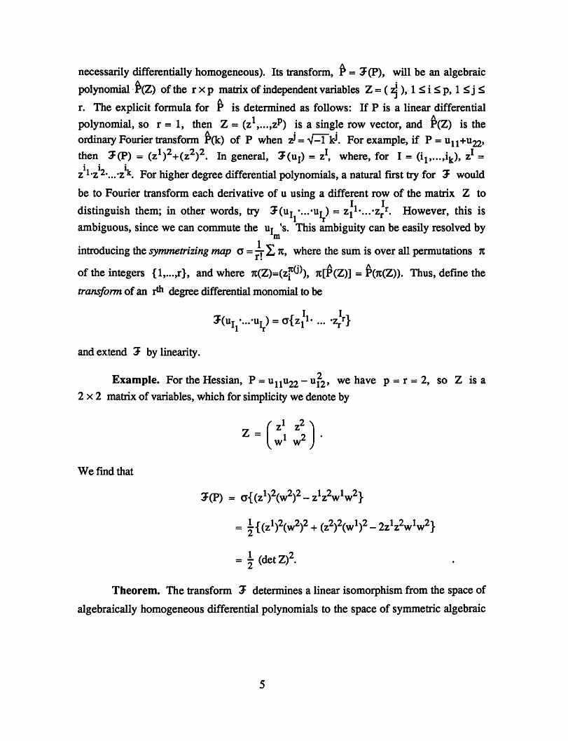
necessarily differentially homogeneous). Its transform, P = ^(P), will be an algebraic

polynomial P(Z) of the rxp matrix of independent variables Z=(zj), l^i^p, 1^j£r. The explicit formula for P is determined as follows: If P is a linear differential

polynomial, so r = 1, then Z = (z},...,z^) is a single row vector, and P(Z) is theordinary Fourier transform P(k) of P when z^ =^f-TkK For example, if P = u11+u22»then ?(P) = (z*)2+(z2)2. In general, JOij) = z1, where, for I = (il9...,ik), z1 =z l-z2\..-z\ For higher degree differential polynomials, a natural first try for 3F wouldbe to Fourier transform each derivative of u using a different row of the matrix Z to

distinguish them; in other words, try 2(uj ,...,Ut ) = Zj1*...^,.1*. However, this isambiguous, since we can commute the uT 's. This ambiguity can be easily resolved by

m

introducing the symmetrizing map a =-r 2 rc, where the sum is overall permutations %

of the integers {l,...,r}, and where n(Z)=(zf®), rc[$(Z)] =£(rc(Z)). Thus, define thetransform of an r* degree differential monomial to be

3:(uIi-...-uIr) =a{z1i-... -z/}

and extend 3- by linearity.

Example. For the Hessian, P=unu22 - u22, we have p =r =2, so Z is a2x2 matrix of variables, which for simplicity we denote by

We find that

Z ='z1 z2^w w

3F(P) = c{(zl)2(v/2)2--z1z2\vlv/2}

= t{(z1)2(w2)2 +(z2)2(wx)2 - 2z1z2w1w2}

=|(detZ)2.

Theorem. The transform J determines a linear isomorphism from the space of

algebraically homogeneous differential polynomials to the space of symmetric algebraic

polynomials of the matrix of variables Z. (By definition, P(Z) is symmetric if rc(P) = P

for all permutations k.)

More generally, if there is more than one dependent variable, so q > 1, then wedefine the transform on differential polynomials which are homogeneous of degree ra in

ua, where r =rj+^.+rq, simply by writing the u's in each differential monomial inascending order, and, instead of using the full symmetrizing map a, just using a =

(Ilrv!) X' k, the sum now being only over those permutations which permute each setof ra rows of Z among themselves. For instance, if P depends quadratically on

derivatives of u1 and linearly on derivatives of u , then r = 3, and the only twopermutations occuring in a are the identity and (12). The isomorphism theorem, with the

proper interpretation of "symmetric", works just as before. (This is equivalent to, but

slightly different from, the procedure used in [2], [14].)

The key to the utility of the transform method is its ability to change differential

operations into algebraic operations. Two particularly important operations are the totalderivatives Dj, and the Euler operator (variational derivative) E from the calculus of

variations, cf. [7]. If L is any linear operator on the space of differential polynomials,

then we let L be the corresponding "transformed" operator on the space of symmetric

polynomials P(Z).

Proposition. The transforms of the totalderivatives Dj and the Euleroperator E

are given by

&£ =(4 +... +zj)-£(Z),

and, letting Zj denote the j* row of Z,

E(P) =$(zv...9zr_v -Zj - ... - z^).

(Note that E(P) has algebraic degree one less than that of P.)

As an immediate corollary, we derive the well-known result, cf. [7], that the kernel

of the Euler operator is the image of the total divergence:

E(P) = 0 if and only if P = Div Q for some p-tuple Q.

Indeed, transforming the above statement, we see that it is equivalent to the trivial algebraic

proposition

fyz!,...,^.!,- zx - ... - zr_l) =0 if and only if £(Z) =^T (zj +... +zf)-^i

for polynomials Qi(Z).

3. The Symbolic Method.

In the special case when each function ua =z* ( ^J'0?**1 *s a homogeneouspolynomial or form of degree m, a differential polynomial P[u] will evaluate to a

polynomial function of the coefficients cf as well as the x's. As such, it will have anumbral representation determined by the classical symbolic method, cf. [8], [9], [10].

Here we will follow Gurevich's notation for symbolic factors of the first and second kind,

as the convention of Kung and Rota in which they are both brackets is rather special to thecase of binary forms (p =2). Thus, if Zj =(z| +... +zP), j=l,...,r, are umbral letters(the reason we use z rather than the more standard Greek letters will be clear presently),

we use the notation

(Zj x) =zj xl+...+zf*P

for the symbolic factors of the first kind, and

[Zji,...,Zj ]=det (z|v ) s det(Zj)

for the symbolic factors of the second kind, or bracketfactors. Note that if we form an

rxp matrix Z out of the letters Zj,...^, then the bracket factor [z,...,Zj] can be

identified with the determinant of the pxp minor Zj consisting ofrows j1,...,jp of Z.

A key observation is that, apart from inessential symbolic factors of the first kind

and a multiplicative constant, the transform of P agrees with the unique symmetric umbral

representation of P. Specifically, we have the following result.

Theorem. Let P[u] be a differential polynomial, which is both differentiallyhomogeneous of degree k and algebraically homogeneous of degree ra in the k^1

derivatives of ua, with r =r^^.+r . Let r(Z) be the transform of P. Let ua(x) be

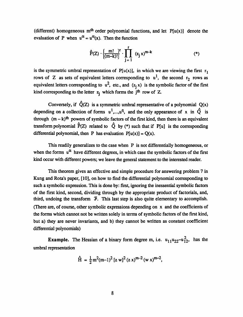
(different) homogeneous m* order polynomial functions, and let P[u(x)] denote theevaluationof P when ua = ua(x). Then the function

to-i^-n<*«r* (*>

is the symmetric umbral representation of P[u(x)], in which we are viewing the first rxrows of Z as sets of equivalent letters corresponding to u1, the second r2 rows asequivalent letters corresponding to u, etc., and (Zj x) is the symbolic factor of the firstkind corresponding to the letter Zj which forms the j* row of Z.

Conversely, if Q(Z) is a symmetric umbral representative of a polynomial Q(x)

depending on a collection of forms u1,...,^, and the only appearance of x in Q isthrough (m- k)* powers of symbolic factors of thefirstkind, then there is anequivalenttransform polynomial P(Z) related to Q by (*) such that if P[u] is the corresponding

differential polynomial, then P has evaluation P[u(x)] = Q(x).

This readily generalizes to the case when P is not differentially homogeneous, or

when theforms ua have different degrees, in which case the symbolic factors of the firstkind occur with different powers; we leave the general statement to the interested reader.

This theorem gives an effective and simple procedure for answering problem 7 in

Kung and Rota's paper, [10], on how to find the differential polynomial corresponding to

such a symbolic expression. This is done by: first, ignoring the inessential symbolic factors

of the first kind, second, dividing through by the appropriate product of factorials, and,third, undoing the transform 3\ This last step is also quite elementary to accomplish.

(There are, of course, other symbolic expressions depending on x and the coefficients of

the forms which cannot not be written solely in terms of symbolic factors of the first kind,

but a) they are never invariants, and b) they cannot be written as constant coefficient

differential polynomials)

Example. The Hessian of a binary form degree m, i.e. ^n^l'Hl9 ^as ^e

umbral representation

ft = i-m2(m-l)2[zw]2(zx)m-2(wx)m-2,

cf. [10; page 70]. Comparing with (*), we see that the corresponding transform

polynomial is just

JP= |[zw]2 = i-(detZ)2,

where Z is the above 2x2 matrix. Thus we recover the standard representation of the

Hessian of a form as a polynomial in its second order derivatives.

As a second example, consider the transvectant (u,u)^4\ which has umbralrepresentation

fl" =\ [z w]4 (z x)"1"4 (w x)m_4.

The corresponding transform polynomial is, according to (*),

K^[zw]4 =̂ (detZ)42-m!2 2-m!2

=(md^ {(zl)4(w2)4 _6(zl)3z2wl(w2)3 +̂ Ift^lfaft_2-mr

- 6zx{z2)\vA)\2 +(z2)4(w!)4 },

It is easy to see that this is the transform of the differential polynomial

„ (m-4)!2 f , _ 2 1r = "^2~" Lullllu2222"" ou1112u1222 +:>U1122J-

If we had done the transvectant (u,v/4* of two different forms of degree m, then wewould recover the classical formula

JF~ Lullllv2222"6u1112v1222+ 10u1122v1122" 6u1222v1112+ U2222V1111J »

cf. [8; page 227]. This clearly demonstrates the power of the transform method for

determining the differential polynomial expressions of formulas from classical invariant

theory.

In fact, the transform approach to classical invariant theory accomplishes more.

Since it works for arbitrary smooth (C°°) functions, not just homogeneous polynomials, it

leads immediately to an invariant theory ofsmooth (or analytic)functions. In this case, the

invariants to be considered are differential polynomials in the functions, which are

unchanged (up to a factor) under the action of the general linear group GL(p). It is not

difficult to see that the induced action of GL(p) on the space of differential polynomials

commutes with the transform. Consequently, the First Fundamental Theorem of Classical

Invariant Theory, [9], [10], immediatelyprovides a classificationof all invariantdifferential

polynomials.

Theorem. A differential polynomial P[u] is an invariant under the general linear

group GL(p) if and only if its transform P(Z) is a polynomial in the symbolic factors of

the second kind, i.e. a bracketpolynomial. In particular, this requires that r, the degree of

algebraic homogeneity of P, be greater than or equal to p, the number of independent

variables, and that r be a polynomial in the determinants of the p x p minors of the r x p

matrix Z.

There are, of course, relations among the invariant differential polynomials, all

stemming from the basic syzygy among the brackets:

P+l

X [zi» •••> zj-i> zj+i> •••' Vil'[zi' wi> ••" wp-i] =°-j = l

However, if the functions ua are homogeneous polynomials, or, more generally,

homogeneous functions of x, then there are additional relations stemming from the syzygy

between the brackets and the symbolic factors of the first kind

p+l

/ f tzi> •••> zj_i> zj+i> •••> zp+i]'(zj> x) = 0,j = l

even though the latter factors do not explicitly appear in the transform representation of P.

We do not have space to go into the full details of the interplay between the invariant

differential polynomials and the classical invariants of homogeneous polynomials, but there

are three points to note. First, there are far more invariant differential polynomials than

classical invariants because we only have "half* the number of syzygies at our disposal in

10

the former case. In particular, the invariantdifferential polynomials arenot an algebraically

finitely generated ideal. Second, the first fact immediately leads to a number of "universal

identities" which are valid for arbitrary homogeneous functions, all of which come from

differential polynomials which give the same classical invariant when evaluated on

homogeneous polynomial functions. The simplest example is the invariant differentialpolynomial whose transform is [z^z^} [z^z^lz^z^], but whose corresponding umbral

representation when u is a form always vanishes. The differential polynomial has the

explicit formula

9 2

ull(u112u222~u122) ~ u12(ulllu222_u112u122) +u22(ulllu122"'u112) = °>

i owhich vanishes for all homogeneous functions u(x ,x ), but is certainly not zero for all

smooth functions u. Finally, the classical invariant^eoretic concept of a perpetuant, [8],[10], which is usually referred to as "an invariant of a form of infinite degree", can be

reinterpreted in this light as an invariant differential polynomial of a homogeneous function

of non-integral degree of homogeneity, i.e. u(A,x) = Xa-u(x), where a is not an integer

(in particular, u is not a polynomial). This is because all the syzygies of the second kindinvolve factors like (a-k), ke Z, so certain relations among bracket polynomials

degenerate when a happens to be integral. These remarks will be treated in greater detail

in a forthcoming paper.

4. Characterization of Homogeneous Divergences.

The solution of problem 1 of the introduction using the transform proceeds as

follows. First, for later reference, we determine the transform of a Jacobian determinant

J = —r r— = det

8(xki,...,xkr)

of derivatives of u. A simple calculation shows that

^Ivax*v

J=̂ -det(ZK)-det(Z'A)

where Z denotes the rxr minor consisting of columns kj,...^ of the matrix Z, and

Z^ denotes the rxr matrix ofmonomials zj which occur in the symmetric powers ofthe matrix Z.

11

Theorem. Let q = 1. Then every differentially homogeneous divergence Q =

Div P is a linear combination of Jacobian determinants of derivatives of u.

Proof.

Consider the transform Q of Q. Using the formula for the transform of the total

derivatives, we see that Q is a divergence if and only if

P

&Z)= ]T (z\ +... +z})-Pi(Z)i=l

A

for polynomials Pj(Z). This means that

Q(Z) =Q(zj,..., Zj.) = 0 whenever Zj + ... + z, = 0,

Zj denoting the i* row of Z. Moreover, differential homogeneity of Q implies that Q

is a homogeneous function of degree k of the rows of Z, so

Q(^lzl> •••> Aj^r) —(A»i* ... 'Aj) •Q (z^ ..., Zj).

Thus we have the stronger condition

Qtzj,..., Zj.) = 0 whenever zx,..., zr are linearly dependent.

If p < r, it is easy to see that there are no nontrivial such polynomials Q. Otherwise, let<& denote the determinantal ideal generated by the r x r minors Z of the r x p matrix

Z. Then the above condition is equivalent to the fact that Q vanishes on the ideal -A*.According to a theorem of Northcott, [13], andMount, [12], *A* is a prime ideal, andso

by the Hilbert Nullstellensatz

&Z) =£(detZK)-RK(Z)K

for some polynomials RK(Z). Finally, we use the fact that Q is symmetric; applying the

symmetrizing map a to the last formula, we can replace RK(Z) by its skew-

symmetrization RK, which is easily seen to be a linear combination of the power

determinants det(Z^ occurring in the transform ofthe Jacobian determinants. Therefore

12

Q is a linear combination of transforms of Jacobian determinants, and hence inverting the

transform proves that Q itself is a linear combination of Jacobian determinants, which

completes the proof of the theorem.

5. Hyperjacobians and Transvectants.

The corresponding problem for homogeneous higher order divergences is

approached in the same manner. We begin by transforming the basic condition

Q = S DjPj,

into the polynomial equation

&Z)= S (z1 +... +zr)I-^I(Z),

where (zj + ... + z,. )l denotes the Ith power of the sum of the rows of Z. Again,differential homogeneity of Q implies that Q is an algebraically homogeneous function of

the rows of Z, so the above condition is equivalent to the condition that Q and all itspartial derivatives up to order k-1, with respect to the variables zj, lie in thedeterminantal ideal -Jl*. In otherwords, Q lies in thek* symbolic power of <A*.

At this point, we require an important result of Trung, [22], (see also DeConcini,

Eisenbud and Procesi, [5]) that for maximal sized minors of a matrix of independent

variables Z, thek* symbolic power of the corresponding determinantal ideal <A* is thesame as the ordinary k* power of Jt*. Therefore, any such Q can be written as a sumof

powers of determinants:

&Z) = £ (det Z1!)-... -(det Z*k) •iH(Z).

Moreover, applying a as before, we find that R^(Z) can be written as a linearcombinations either of power determinants, det(Z ), if k is odd, or power permanants,

perm( Zr), if k is even. Thus, to complete the characterization of homogeneous higher

order divergences, we need to know which differential polynomials transform to

(det ZIl)-...-(det ZIk)*(det ZA), if k is odd,

or

13

(det ZXl)\..-(det zV(perm ZA), if k is even.

The answer is given by the theory of hyperjacobians, [14]. Rather than give the

most general definition of a hyperjacobian, which is a generalization of the classical concept

of a Jacobian determinant, we present the second degree examples, from which the general

definition can easily be guessed.

Example. A first order hyperjacobian is simply a Jacobian determinant, e.g.

3(u,v)a, l 2, =uiv2-u2vl-d(x ,x )

A second order hyperjacobian is obtained from a first order one by a similar determinantal

formula:

a2(u,v) 3(U3>V4) d(u4>v3)a, 1 2^, 3 4x = a/ 1 2v - a, 1 L = u13v24-u23v14-u14v23 +u24v13«d(x ,x )d(x ,x ) d(x ,x ) d(x ,x )

In particular,

32(u,v) «—Wj = u11v22-2u12v12 + u22v11d(x ,x )

is a multiple of the second transvectant of u and v, and

a(x1,x2)2-2(UllU22"Ul2)

agrees, up to a factor, with the Hessian of u. Similarly, third order hyperjacobians are

constructed from second order hyperjacobians by the same determinantal procedure; for

example

32(u,v) 32(ui»V2) d2(u2»vi) o oa, 1 2x2 = a/ 1 2x2 " a/ 1 2x2 =ulllv222_:Ju112v122 +:)u122v112""u222vllld(x ,x ) d(x ,x ) d(x ,x )

is a multiple of the third transvectant of u and v, cf. [9; page 227]. In general, if u and v

are homogeneous polynomials, the k* transvectant (u,v)^ isjust amultiple of the k1*1order hyperjacobian 9k(u,v)/9(x1,x ) .

The general formula for the hyperjacobian

14

aV ur)d(xl xS... 3(xrai x^)

is found inductively on k, using a similar determinantal construction. They can also be

constructed using the theory of higher dimensional determinants of higher order Jacobian

"matrices", cf. [14]. They provide the natural generalization of the notion of transvectant to

higher dimensional problems. Furthermore, their transforms are precisely what is required

to complete the analysis of higher order divergences, so we have the following result:

Theorem. A differential polynomial Q is a k* orderdivergence if andonly if itis a linearcombination of k* orderhyperjacobians of derivatives of u.

In particular, any k* order transvectant is a k* orderdivergence, a fact thatdoes

not appear to have previously been noticed in the literature.

6. Differential Hyperforms.

Although we now know that any k* order hyperjacobian can bewritten as a k*order divergence, the determination of exactly how to do this is a non-trivial task. One

solution to this algebraic problem has resulted in the development of a new theory of higher

order differential forms, or "hyperforms". The motivation for this is the observation that

the divergence identity for the ordinary Jacobian determinant is equivalent to the differential

form identity

du a dv = d(u-dv).

The goal is to develop a theory of differential forms so that the identity

—^2 =D?(-U2V2) +D1D2(u1V2 +u2v1) +b^(-u1v1)d(x ,x )

for the second order hyperjacobian (second transvectant) translates into an identity of the

form

d^ *d2v =d2(du * dv)

for second order hyperforms. Such a thory has been developed over Euclidean space in the

unpublished paper [15], and we here summarize its principal ingredients.

15

Let X denote a Young diagram, or shape, and |A,| the number of boxes in X.Given a finite dimensional real vector space V, we let L^V denote the correspondingirreducible representation space of the general linear group GL(V); L^ is known as the

Schur functor (or shape functor). See [1], [11], [21], for the general theory of Schur

functors. Pieri's formula is

where the direct sum is over all shapes fi containing X and having precisely one box

more than X. For notation, we write Xc\i when X is contained in \i, andwrite \i\Xfor the skew shape consisting of all boxes of |X which do not lie in X; thus the above

direct sum would be over all \i z> Xwith \\i\X\ =1. This formula implies the existence of

functorialmaps

cp^Val^V-^V,

for any such 7^ |i, which are uniquely defined up to scalarmultiple.

Example. Recall first that the Schur space L^V can be identified with thequotient space of the tensor product of the symmetric powers G^ V <8>... ®Oi V under

the two-sided ideal generated by the Young relations

Sxj® (xjOy),

A

for Xj, ..., Xp+1 e V, y e G^V, and where Xj = Xj O... Oxj^Ox^jO... OXp+1.Therefore, each element co of L^V can be identified with an equivalence class inG^ V ®... <8> Gi V, and we can use any element of this equivalence class torepresent co.

With this inmind we will write elements of L^V as if they were in G^ V <8>... ®Oi V,

but with the understanding that we are allowed to replace such a representative by any

equivalent element as prescribed by the Young relations.

We can write down the explicit formulas for the Pieri maps (pjf. The easiest

approach is to present a few specialcases, from which the general formulacan be deduced.First, if X= (k,t), k >I, and \x=(k+l,t), then

16

<$(v®(x®y)) = (vOx)®y + 2j (xGyj) ®(vOyxj).i= 1

If H= (k,Ul) (so k > JL),

(pjjj(v ®(x®y)) =x ®(vO y),

while if |X = (k,JL,l), then

(pJJ;(v ®(x ®y)) =x ®y ®v.

Similarly, if A,=(k,£,m), k >H£ m, and |i = (k+l,JL,m), then

I

<pj)J(v ®(x ®y®z)) = (vOx) ®y +—r— ^ (x Ovj) ®(vOVj) ®z+1= 1

m H m

+l^nT3X (x0zP®y®^^ +i^-^mT3XX (xOyf)® (y^)® (vOz>j=l K^z i=l j=1

while if n=(k,H+l,m), so k > H, then

m

1 X"1 A<pjjj(v ®(x ®y®z)) =x®(vOy) ®z+ ^ x®(yOz:) ®(vOZj).m+ j=i

Also, for |j. = (k,JL,m+l) (so i >m) and |a=(k,JL,m,l) we have

(pJJ(v ®(x ®y ®z)) =x®y ®(vO z), and q>Jf(v ®(x®y®z)) =x®y®z®v

respectively. The general formula appears in [15].

In any of the above formulas, we could multiply <pjf by a constant cjj, without

affecting the functoriality. Itturns out that one can choose constants cjf in such away that

the resulting Pieri products

v* co =cj(; •(p5f(v ®co), v € V, co e L^V, v *co € L^V,

17

commute in the sense that v * v * co is unambiguously defined as an elementof LyV

whenever Xczv and |v\X.| = 2, in which case the two * products can be computed in

two distinct ways, depending on which box is added on to X first. One possible choice of

the factors cJJ is the following: if X=(a-j,...,^), and p =(A^,..., 7^_lt Xj+1, Xj+1,...,A^), then set

* =1

v.

X.J + n j = 1

n+l

(^-Xj+j-D n x * . .. kj^k=j+l A,j-A,k + k-j

1 , j = n+l

where A^+1 =0 by convention. For instance, if X=(k,£), |i=(k+l,&), then cjj1 =r^r,k-4,+1while if |i=(k,JL+l), cjf = » . Finally, let v be a fixed nonzero vector in V, and

define the map \|/JJ: L^V -> L^V by

\|^(co) =v * co =dj •<pJJ(v ®co), co e L^V.

Lemma. Let X. c p <z v, and ^c^i'cv' be shapes, with |p\X|=l, |pAX|=l,

and |v\|ihl, |v\|Lt'|=l (so |v\X|=2). Then

commute and serve to unambiguously define amap \|^ from L^V to LyV.

By the lemma, it is easy to see that, given v e V, we can uniquely define a map

\|/j{: L^V -> L„V for any shape p containing X; if ||i\X|=m, then we define yjj by m-fold composition of the basic Pieri maps, adding on one box at a time. The lemma assures

us that it does not matter in which order the boxes are added on.

Theorem. Let 0* ve V, and let y£: L^V -» L^V, Xc p., be the corresponding maps ofSchur spaces. Then the maps \|/j{ define an exact hypercomplex over V.

Here "hypercomplex", which is a generalization of the usual homological algebraic concept

of a complex, means that these maps satisfy the two properties of

18

a) Commutativity: Whenever Xc p and pc v, then \|/^= \|/J[0\|^.

b) Closure: Whenever X c v and v\X contains two or more boxes in any one

column, then \j;^= 0.

Furthermore, the Schur hypercomplex is exact, meaning that

c) Exactness: Suppose Xcp and pcv, and p\X and v\p each consist of only

one row of boxes, and v\X, which consists of two rows of boxes, has two boxes in one

and only one column. Then, yX(co) =0 for co e L„V if and only if co=\|/£(9) for some

eei^v.

(There is amore general statement ofexactness which characterizes the kernel of \j/^ forany pcv, but this is a little harder to state, and the above notion of exactness is sufficient

for this more general version to hold; see [15] for details.)

Contained in the Schur hypercomplex, corresponding to the shapes with only one

column of boxes, is the standard exterior complex co —» vaco, co e AkV, and in this

case, closure and exactness reduce to their more familiar counterparts.

What we are really interested in is the differential counterpart of the Schur

hypercomplex. At present, the construction has only been carried out for open subsets M

of Euclidean space IRP, but extensions to arbitrary smooth manifolds are possible, once

certain technical details regarding changes of variable have been overcome. Let T*M bethe cotangent bundle of M, with T*M |x, which will play the role of our vector space V,

denoting the cotangent space of M at x e M. LetS^ |x=L^T*M|x be the corresponding

Schur space at x, with 2^ the corresponding "Schur bundle", constructed in the exact

same manner as the exterior powers AkT*M, which are just special cases when X hasonly one column of boxes. A differential hyperform of shape X will be a section of S^.

More explicitly, let dx1,...,dxp be the standard basis of T*M. Then corresponding toevery Young tableau of shape X whose entries are chosen from the set of indices{l,...,p}, there is an element dxT of S^. The elements dxT corresponding to standard

tableaux form abasis of S^, cf. [1]. (Here standard means that therows of the tableau are

nondecreasing and the columns strictly increasing.) Therefore any differential hyperform

can be written in the form

19

co = 2 fjOO *dxT,

where the sum is over all standard tableaux of shape X. If X<= p and p differs from X

by only one box, then we define the differential of CO to be the differential hyperform

dco =djjco = 2 dfT(x) *dxT = X cjjj •<p£(dfT(x) ®dxT),

where dfT € T*M denotes the ordinary differential of the coefficient function fT. The

algebraic commutativity lemma immediately implies the commutativity of the differentials:Let X c p c v, and X c p' c v be shapes, with |p\X|=l, |p'\X|=l, and |v\p|=l,

|v\p'|=l (so |v\X|=2). Then cl^ ° d£ = cL^ °d£ commute and serve to unambiguouslydefine asecond order differential d% from S^ to Sv. Therefore, by composition, we can

define adifferential d=dJJ: E^ ->S„ whenever Xc p. The main result from [15] is:

Theorem. Let M c IRP be a star-shaped domain. Then the differential

hypercomplex defined by the differentials djf: S^ —> 5„ on hyperforms is an exacthypercomplex.

Contained within the differential hypercomplex, corresponding to those shapes with

only one column, is the ordinary deRham complex over M, where closure and exactness

reduce to their usual meanings. There are also a host of other interesting subcomplexes of

the full hypercomplex, but space precludes us presenting this in any detail here. If M is

not star-shaped, then one can use the failure of the differential hypercomplex to be exact to

define new "hypercohomology" over M, but this has not been investigated at all.

If X= 0 is the "empty shape", then S^|x= IR, and a "O-hyperform" is just anordinary real-valued function. If p = (k) consists of a single row, so S„ = GkT*M is

the k* symmetric power of T*M, then dfj-u =dhi is just the k* differential of thefunction u, i.e.

dku=Z(i)ui-dxi'

the sumbeing overall multi-indices I of order k, with Uj denoting the corresponding

k^ orderpartial derivative. Oneimmediate consequence of theexactness of thedifferentialhypercomplex is that, provided M is star-shaped, a section co of S„=GkT*M is a k*

20

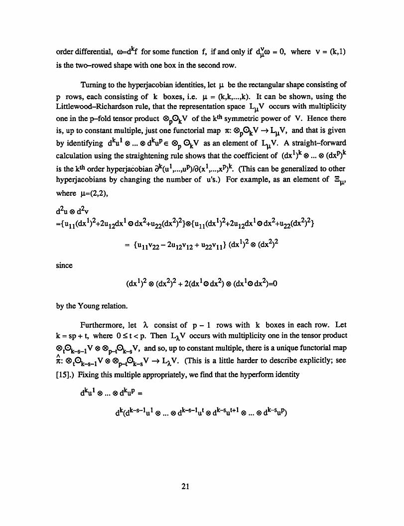
order differential, co=dkf for some function f, ifand only if d?[co =0, where v =(k,l)is the two-rowed shape with one box in the second row.

Turning to the hyperjacobian identities, let p be the rectangularshape consisting of

p rows, each consisting of k boxes, i.e. p = (k,k,...,k). It can be shown, using theLittiewood-Richardson rule, that the representation space L„V occurs with multiplicity

one in the p-fold tensor product G^O^V of the k* symmetric power of V. Hence thereis, up to constant multiple, just one functorial map n: ^pO^V -» L„V, and that is givenby identifying d^i1 ®... ®d^ e <SL O^V as an element of L„V. A straight-forwardcalculation using the straightening rule shows that the coefficient of (dx1) ®... ®(dx1*)is the k* order hyperjacobian dk(u1,...,up)/3(x1,...,xp)k. (This can be generalized to otherhyperjacobians by changing the number of u's.) For example, as an element of S^,

where p=(2,2),

d2u ®d2v

={ux^dx^^u^dx10 dx2+u22(dx2)2}®{u11(dx1)2+2u12dx10 dx2+u22(dx2)2}

= fullv22 " 2ul2vl2 +u22vll> (dxl)2 ®(d*2)2

since

(dx1)2 ®(dx2)2 +2(dx1<D dx2) ®(dx^dx2)^

by the Young relation.

Furthermore, let X consist of p - 1 rows with k boxes in each row. Letk =sp +t, where 0^t<p. Then L^V occurs withmultiplicity one in the tensor product

®t®k-s-lv ®®pHpk-sV' m& so» UPto constant multiple, there is aunique functorial map7t: ®t®k-s-lv ®®pnPk-sV ""* LXV* (This is a little harder t0 describe explicitly; see[15].) Fixing this multiple appropriately, we find that the hyperform identity

dV ® ... ®dV =

dk(dk-8-V ®... ®dk-*"V ®dk"8ut+1 ®... ®dk_sup)

21

is equivalent to the expression of the above k* order hyperjacobian as a k* orderdivergence. Here we are identifying the hyperform in parenthesis with its image in S^

under the map %, and d =djjj.

Example. For the Hessian, we need to look at the identity

d2u ®d2v = d2(du ®dv),

where d u®d2v e Sr2 2,, and du ®dv e Sr2,. We find

du ®dv =-^duOdv =-^{u^dx1)2 +(u2v1+u1v2)dx1 Odx2 +u2v2(dx2)2}

and

d2(du ®dv) =-^d^u^) *(dx1)2 +d2(u2v1+u1v2) *dx1 Odx2 +d2(u2V2) *(dx2)2}

={-D^u^) +D^^v^u^) -D21(u2v2)} •(dx1)2 ®(dx2)2,

and we recover the second order transvectant identity. See [14], [15], for further identities

of this type.

References

[1] Akin, K., Buchsbaum, D. A. and Weyman, J., Schur functors and Schurcomplexes, Adv. in Math. 44 (1982), 207-278.

[2] Ball, J. M., Currie, J.C. and Olver, P.J., Null Lagrangians, weak continuity, andvariational problems of arbitrary order, /. Func. Anal. 41 (1981), 135-174.

[3] Coleman, B.D. and Noll, W., The thermodynamics of elastic materials with heatconduction and viscosity, Arch. Rat. Mech. Anal. 13 (1963), 167-178.

[4] Cushman, R. and Sanders, J.A., Nilpotent normal forms and representation theoryof sl(2,R), Univ. of Amsterdam, Report #301, 1985.

[5] DeConcini, C, Eisenbud, D. and Procesi, C, Young diagrams and determinantalvarieties, Invent. Math. 56 (1980), 129-165.

22

[6] Dunn, J.E. and Serrin, J., On the thermomechanics of interstitial working, Arch.Rat. Mech. Anal. 88 (1985), 95-133.

[7] Gel'fand, I.M. and Dikii, L.A., Asymptotic behaviour of the resolvent of Sturm-Liouville equations and the algebra of the Korteweg-deVries equations,Russ. Math. Surveys 30 (1975), 77-113.

[8] Grace, J.H. and Young, A., TheAlgebra ofInvariants, Cambridge Univ. Press,Cambridge, 1903.

[9] Gurevich, G.B., Foundations ofthe Theory ofAlgebraic Invariants, P. NoordhoffLtd., Groningen, Holland, 1964.

[10] Kung, J.P.S. and Rota, G.-C., The invariant theory of binary forms, Bull. Amer.Math. Soc. 10 (1984), 27-85.

[11] Lascoux, A. Syzygies des varietSs determinantales, Adv. in Math. 30 (1978), 202-237.

[12] Mount, K.R., A remark on determinantal loci, /. London Math. Soc. 42 (1967),595-598.

[13] Northcott, D.G., Some remarks on the theory of ideals defined by matrices, Quart.J. Math. Oxford 85 (1963), 193-204.

[14] Olver, P.J., Hyperjacobians, determinantal ideals and weak solutions to variationalproblems, Proc. Roy. Soc. Edinburgh 95A (1983), 317-340.

[15] Olver, P.J., Differential hyperforms I, Univ. of Minn. Math. Report 82-101,1983.

[16] Olver, P.J., Conservation laws and null divergences, Math. Proc. Camb. Phil.Soc. 94 (1983), 529-540.

[17] Olver, P.J., Conservation laws and null divergences II. Nonnegative divergences,Math. Proc. Camb. Phil. Soc. 97 (1985), 511-514.

[18] Olver, P.J., Applications ofLie Groups to DifferentialEquations, Graduate Textsin Mathematics, vol. 107, Springer-Verlag, New York, 1986.

[19] Shakiban, C, A resolution of the Euler operator II, Math. Proc. Camb Phil. Soc.89 (1981), 501-510.

[20] Shakiban, C. An invariant theoretic characterization of conservation laws, Amer. J.Math. 104 (1982), 1127-1152.

[21] Towber, J., Two new functors from modules to algebras, /. Algebra 47 (1977),80-104.

[22] Trung, N.V., On the symbolic powers of determinantal ideals,/. Algebra 58(1979), 361-379.

23