1

Invariant Scattering Convolution NetworksJoan Bruna and Stephane Mallat

CMAP, Ecole Polytechnique, Palaiseau, France

Abstract —A wavelet scattering network computes a translation invari-ant image representation, which is stable to deformations and preserveshigh frequency information for classification. It cascades wavelet trans-form convolutions with non-linear modulus and averaging operators. Thefirst network layer outputs SIFT-type descriptors whereas the next layersprovide complementary invariant information which improves classifica-tion. The mathematical analysis of wavelet scattering networks explainimportant properties of deep convolution networks for classification.

A scattering representation of stationary processes incorporateshigher order moments and can thus discriminate textures having sameFourier power spectrum. State of the art classification results are ob-tained for handwritten digits and texture discrimination, with a Gaussiankernel SVM and a generative PCA classifier.

Index Terms —Classification, Convolution networks, Deformations, In-variants, Wavelets

1 INTRODUCTION

A major difficulty of image classification comes fromthe considerable variability within image classes and theinability of Euclidean distances to measure image simi-larities. Part of this variability is due to rigid translations,rotations or scaling. This variability is often uninforma-tive for classification and should thus be eliminated.In the framework of kernel classifiers [33], the distancebetween two signals x and x′ is defined as a Euclideandistance ‖Φx − Φx′‖ applied to a representation Φxof each x. Variability due to rigid transformations areremoved if Φ is invariant to these transformations.

Non-rigid deformations also induce important vari-ability within object classes [17], [3]. For instance, inhandwritten digit recognition, one must take into ac-count digit deformations due to different writing styles[3]. However, a full deformation invariance would re-duce discrimination since a digit can be deformed into adifferent digit, for example a one into a seven. The rep-resentation must therefore not be deformation invariant.It should linearize small deformations, to handle themeffectively with linear classifiers. Linearization meansthat the representation is Lipschitz continuous to defor-mations. When an image x is slightly deformed into x′

then ‖Φx − Φx′‖ must be bounded by the size of thedeformation, as defined in Section 2.

• This work is funded by the French ANR grant BLAN 0126 01.

Translation invariant representations can be con-structed with registration algorithms [34], autocorrela-tions or with the Fourier transform modulus. However,Section 2.1 explains that these invariants are not stableto deformations and hence not adapted to image clas-sification. Trying to avoid Fourier transform instabilitiessuggests replacing sinusoidal waves by localized wave-forms such as wavelets. However, wavelet transformsare not invariant but covariant to translations. Build-ing invariant representations from wavelet coefficientsrequires introducing non-linear operators, which leadsto a convolution network architecture.

Deep convolution networks have the ability to buildlarge-scale invariants, which seem to be stable to defor-mations [20]. They have been applied to a wide range ofimage classification tasks. Despite the successes of thisneural network architecture, the properties and optimalconfigurations of these networks are not well under-stood, because of cascaded non-linearities. Why usemultiple layers ? How many layers ? How to optimizefilters and pooling non-linearities ? How many internaland output neurons ? These questions are mostly an-swered through numerical experimentations that requiresignificant expertise.

We address these questions from mathematical andalgorithmic point of views, by concentrating on a par-ticular class of deep convolution networks, defined bythe scattering transforms introduced in [24], [25]. A scat-tering transform computes a translation invariant repre-sentation by cascading wavelet transforms and moduluspooling operators, which average the amplitude of it-erated wavelet coefficients. It is Lipschitz continuous todeformations, while preserving the signal energy [25].Scattering networks are described in Section 2 and theirproperties are explained in Section 3. These proper-ties guide the optimization of the network architectureto retain important information while avoiding uselesscomputations.

An expected scattering representation of stationaryprocesses is introduced for texture discrimination. As op-posed to the Fourier power spectrum, it gives informa-tion on higher order moments and can thus discriminatenon-Gaussian textures having the same power spectrum.Scattering coefficients provide consistent estimators ofexpected scattering representations.

2

Classification applications are studied in Section 4.Classifiers are implemented with a Gaussian kernel SVMand a generative classifier, which selects affine spacemodels computed with a PCA. State-of-the-art resultsare obtained for handwritten digit recognition on MNISTand USPS databases, and for texture discrimination.These are problems where translation invariance, station-arity and deformation stability play a crucial role. Soft-ware is available at www.cmap.polytechnique.fr/scattering.

2 TOWARDS A CONVOLUTION NETWORK

Small deformations are nearly linearized by a representa-tion if the representation is Lipschitz continuous to theaction of deformations. Section 2.1 explains why highfrequencies are sources of instabilities, which preventstandard invariants to be Lipschitz continuous. Sec-tion 2.2 introduces a wavelet-based scattering transform,which is translation invariant and Lipschitz relativelyto deformations. Section 2.3 describes its convolutionnetwork architecture.

2.1 Fourier and Registration Invariants

A representation Φx is invariant to global translationsxc(u) = x(u − c) by c = (c1, c2) ∈ R2 if

Φxc = Φx . (1)

A canonical invariant [17], [34] Φx = x(u−a(x)) registersx with an anchor point a(x), which is translated whenx is translated: a(xc) = a(x) + c. It is therefore invariant:Φxc = Φx. For example, the anchor point may be afiltered maximum a(x) = argmaxu |x ⋆ h(u)|, for somefilter h(u).

The Fourier transform modulus is another exampleof translation invariant representation. Let x(ω) be theFourier transform of x(u). Since xc(ω) = e−ic.ω x(ω),it results that |xc| = |x| does not depend upon c.The autocorrelation Rx(v) =

∫x(u)x(u − v)du is also

translation invariant: Rx = Rxc.To be stable to additive noise x′(u) = x(u) + ǫ(u), we

need a Lipschitz continuity condition which supposesthat there exists C > 0 such that for all x and x′

‖Φx′ − Φx‖ ≤ C ‖x′ − x‖ ,

where ‖x‖2 =∫|x(u)|2 du. The Plancherel formula

proves that the Fourier modulus Φx = |x| satisfies thisproperty with C = 2π.

To be stable to deformation variabilities, Φ must alsobe Lipschitz continuous to deformations. A small deforma-tion of x can be written xτ (u) = x(u − τ(u)), whereτ(u) is a non-constant displacement field which deformsthe image. The deformation gradient tensor ∇τ(u) is amatrix whose norm |∇τ(u)| measures the deformationamplitude at u and supu |∇τ(u)| is the global defor-mation amplitude. A small deformation is invertibleif |∇τ(u)| < 1 [1]. Lipschitz continuity relatively to

deformations is obtained if there exists C > 0 such thatfor all τ and x

‖Φxτ − Φx‖ ≤ C ‖x‖ supu

|∇τ(u)| , (2)

where ‖x‖2 =∫|x(u)|2 du. This property implies global

translation invariance, because if τ(u) = c then ∇τ(u) =0, but it is much stronger.

If Φ is Lipschitz continuous to deformations τ thenthe Radon-Nykoym property proves that the map whichtransforms τ into Φxτ is almost everywhere differen-tiable in the sense of Gateau [22]. It means that forsmall deformations, Φx − Φxτ is closely approximatedby a bounded linear operator of τ , which is the Gateauderivative. Deformations are thus linearized by Φ, whichenables linear classifiers to effectively handle deforma-tion variabilities in the representation space.

A Fourier modulus is translation invariant and stableto additive noise but unstable to small deformations athigh frequencies. Indeed, | |x(ω)| − |xτ (ω)| | can be arbi-trarily large at a high frequency ω, even for small defor-mations and in particular for a small dilation τ(u) = ǫu.As a result, Φx = |x| does not satisfy the deformationcontinuity condition (2) [25]. The autocorrelation Φx =

Rx satisfies Rx(ω) = |x(ω)|2. The Plancherel formulathus proves that it has the same instabilities as a Fouriertransform:

‖Rx−Rxτ‖ = (2π)−1‖|x|2 − |xτ |2‖ .

Besides deformation instabilities, a Fourier modulusand an autocorrelation looses too much information.For example, a Dirac δ(u) and a linear chirp eiu2

aretotally different signals having Fourier transforms whosemoduli are equal and constant. Very different signalsmay not be discriminated from their Fourier modulus.

A registration invariant Φx(u) = x(u − a(x)) carriesmore information than a Fourier modulus, and charac-terizes x up to a global absolute position information[34]. However, it has the same high-frequency instabilityas a Fourier transform. Indeed, for any choice of anchorpoint a(x), applying the Plancherel formula proves that

‖x(u− a(x))− x′(u− a(x′))‖ ≥ (2π)−1 ‖|x(ω)| − |x′(ω)|‖ .

If xτ = xτ , the Fourier transform instability at highfrequencies implies that Φx = x(u−a(x)) is also unstablewith respect to deformations.

2.2 Scattering Wavelets

A wavelet transform computes convolutions with di-lated and rotated wavelets. Wavelets are localized wave-forms and are thus stable to deformations, as opposedto Fourier sinusoidal waves. However, convolutions aretranslation covariant, not invariant. A scattering trans-form builds non-linear invariants from wavelet coeffi-cients, with modulus and averaging pooling functions.

Let G be a group of rotations r of angles 2kπ/K for0 ≤ k < K . Two-dimensional directional wavelets are

3

obtained by rotating a single band-pass filter ψ by r ∈ Gand dilating it by 2j for j ∈ Z

ψλ(u) = 2−2jψ(2−jr−1u) with λ = 2−jr . (3)

If the Fourier transform ψ(ω) is centered at a frequencyη then ψ2−jr(ω) = ψ(2jr−1ω) has a support centered at2−jrη, and a bandwidth proportional to 2−j . The indexλ = 2−jr gives the frequency location of ψλ and itsamplitude is |λ| = 2−j .

The wavelet transform of x is x ⋆ ψλ(u)λ. It is aredundant transform with no orthogonality property.Section 3.1 explains that it is stable and invertible if thewavelet filters ψλ(ω) cover the whole frequency plane.On discrete images, to avoid aliasing, we only capturefrequencies in the circle |ω| ≤ π inscribed in the imagefrequency square. Most camera images have negligibleenergy outside this frequency circle.

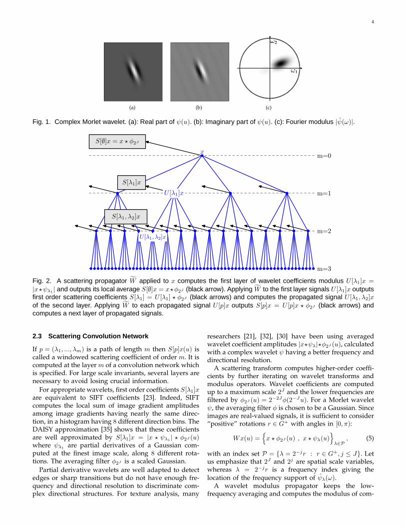
Let u.u′ and |u| denote the inner product and normin R2. A Morlet wavelet ψ is an example of complexwavelet given by

ψ(u) = α (eiu.ξ − β) e−|u|2/(2σ2) ,

where β ≪ 1 is adjusted so that∫ψ(u) du = 0. It’s

real and image parts are nearly quadrature phase filters.Figure 1 shows the Morlet wavelet with σ = 0.85 andξ = 3π/4, used in all classification experiments.

A wavelet transform commutes with translations, andis therefore not translation invariant. To build a transla-tion invariant representation, it is necessary to introducea non-linearity. If Q is a linear or non-linear operatorwhich commutes with translations, then

∫Qx(u) du is

translation invariant. Applying this to Qx = x⋆ψλ givesa trivial invariant

∫x ⋆ ψλ(u) du = 0 for all x because∫

ψλ(u) du = 0. If Qx = M(x ⋆ ψλ) and M is linearand commutes with translations then the integral stillvanishes. This shows that computing invariants requiresto incorporate a non-linear pooling operator M , butwhich one ?

To guarantee that∫M(x ⋆ψλ)(u) du is stable to defor-

mations, we want M to commute with the action of anydiffeomorphism. To preserve stability to additive noisewe also want M to be nonexpansive: ‖My − Mz‖ ≤‖y−z‖. If M is a nonexpansive operator which commuteswith the action of diffeomorphisms then one can prove[7] that M is necessarily a pointwise operator. It meansthat My(u) is a function of the value y(u) only. Tobuild invariants which also preserve the signal energyrequires to choose a modulus operator over complexsignals y = yr + i yi:

My(u) = |y(u)| = (|yr(u)|2 + |yi(u)|2)1/2 . (4)

The resulting translation invariant coefficients are thenL

1(R2) norms

‖x ⋆ ψλ‖1 =

∫|x ⋆ ψλ(u)| du .

The L1(R2) norms ‖x ⋆ ψλ‖1λ form a crude signal

representation, which measures the sparsity of wavelet

coefficients. The loss of information does not comefrom the modulus which removes the complex phaseof x ⋆ ψλ(u). Indeed, one can prove [38] that x can bereconstructed from the modulus of its wavelet coeffi-cients |x⋆ψλ(u)|λ, up to a multiplicative constant. Theinformation loss comes from the integration of |x⋆ψλ(u)|,which removes all non-zero frequencies. These non-zerofrequencies are recovered by calculating the waveletcoefficients |x⋆ψλ1

|⋆ψλ2(u)λ2

of |x⋆ψλ1|. Their L

1(R2)norms define a much larger family of invariants, for allλ1 and λ2:

‖|x ⋆ ψλ1| ⋆ ψλ2

‖1 =

∫||x ⋆ ψλ1

(u)| ⋆ ψλ2| du .

More translation invariant coefficients can be com-puted by further iterating on the wavelet transformand modulus operators. Let U [λ]x = |x ⋆ ψλ|. Anysequence p = (λ1, λ2, ..., λm) defines a path, along whichis computed an ordered product of non-linear and non-commuting operators:

U [p]x = U [λm] ... U [λ2]U [λ1]x = | ||x⋆ψλ1|⋆ψλ2

| ... |⋆ψλm| ,

with U [∅]x = x. A scattering transform along the path pis defined as an integral, normalized by the response ofa Dirac:

Sx(p) = µ−1p

∫U [p]x(u) du with µp =

∫U [p]δ(u) du .

Each scattering coefficient Sx(p) is invariant to a trans-lation of x. We shall see that this transform has manysimilarities with the Fourier transform modulus, whichis also translation invariant. However, a scattering isLipschitz continuous to deformations as opposed to theFourier transform modulus.

For classification, it is often better to compute localizeddescriptors which are invariant to translations smallerthan a predefined scale 2J , while keeping the spatialvariability at scales larger than 2J . This is obtained bylocalizing the scattering integral with a scaled spatialwindow φ2J (u) = 2−2Jφ(2−Ju). It defines a windowedscattering transform in the neighborhood of u:

S[p]x(u) = U [p]x ⋆ φ2J (u) =

∫U [p]x(v)φ2J (u− v) dv ,

and hence

S[p]x(u) = | ||x ⋆ ψλ1| ⋆ ψλ2

| ... | ⋆ ψλm| ⋆ φ2J (u) ,

with S[∅]x = x ⋆ φ2J . For each path p, S[p]x(u) isa function of the window position u, which can besubsampled at intervals proportional to the window size2J . The averaging by φ2J implies that if xc(u) = x(u− c)with |c| ≪ 2J then the windowed scattering is nearlytranslation invariant: S[p]x ≈ S[p]xc. Section 3.1 provesthat it is also stable relatively to deformations.

4

(a) (b) (c)

Fig. 1. Complex Morlet wavelet. (a): Real part of ψ(u). (b): Imaginary part of ψ(u). (c): Fourier modulus |ψ(ω)|.

m=0

m=1

m=2

m=3

x

U [λ1]x

S[∅]x = x ⋆ φ2J

U [λ1, λ2]x

S[λ1]x

S[λ1, λ2]x

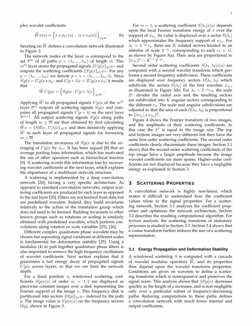
Fig. 2. A scattering propagator W applied to x computes the first layer of wavelet coefficients modulus U [λ1]x =

|x⋆ψλ1| and outputs its local average S[∅]x = x⋆φ2J (black arrow). Applying W to the first layer signals U [λ1]x outputs

first order scattering coefficients S[λ1] = U [λ1] ⋆ φ2J (black arrows) and computes the propagated signal U [λ1, λ2]x

of the second layer. Applying W to each propagated signal U [p]x outputs S[p]x = U [p]x ⋆ φ2J (black arrows) andcomputes a next layer of propagated signals.

2.3 Scattering Convolution Network

If p = (λ1, ..., λm) is a path of length m then S[p]x(u) iscalled a windowed scattering coefficient of order m. It iscomputed at the layer m of a convolution network whichis specified. For large scale invariants, several layers arenecessary to avoid losing crucial information.

For appropriate wavelets, first order coefficients S[λ1]xare equivalent to SIFT coefficients [23]. Indeed, SIFTcomputes the local sum of image gradient amplitudesamong image gradients having nearly the same direc-tion, in a histogram having 8 different direction bins. TheDAISY approximation [35] shows that these coefficientsare well approximated by S[λ1]x = |x ⋆ ψλ1

| ⋆ φ2J (u)where ψλ1

are partial derivatives of a Gaussian com-puted at the finest image scale, along 8 different rota-tions. The averaging filter φ2J is a scaled Gaussian.

Partial derivative wavelets are well adapted to detectedges or sharp transitions but do not have enough fre-quency and directional resolution to discriminate com-plex directional structures. For texture analysis, many

researchers [21], [32], [30] have been using averagedwavelet coefficient amplitudes |x⋆ψλ|⋆φ2J (u), calculatedwith a complex wavelet ψ having a better frequency anddirectional resolution.

A scattering transform computes higher-order coeffi-cients by further iterating on wavelet transforms andmodulus operators. Wavelet coefficients are computedup to a maximum scale 2J and the lower frequencies arefiltered by φ2J (u) = 2−2Jφ(2−Ju). For a Morlet waveletψ, the averaging filter φ is chosen to be a Gaussian. Sinceimages are real-valued signals, it is sufficient to consider“positive” rotations r ∈ G+ with angles in [0, π):

Wx(u) =x ⋆ φ2J (u) , x ⋆ ψλ(u)

λ∈P

, (5)

with an index set P = λ = 2−jr : r ∈ G+, j ≤ J. Letus emphasize that 2J and 2j are spatial scale variables,whereas λ = 2−jr is a frequency index giving thelocation of the frequency support of ψλ(ω).

A wavelet modulus propagator keeps the low-frequency averaging and computes the modulus of com-

5

plex wavelet coefficients:

Wx(u) =x ⋆ φ2J (u) , |x ⋆ ψλ(u)|

λ∈P

. (6)

Iterating on W defines a convolution network illustratedin Figure 2.

The network nodes of the layer m correspond to theset Pm of all paths p = (λ1, ..., λm) of length m. Thismth layer stores the propagated signals U [p]xp∈Pm andoutputs the scattering coefficients S[p]xp∈Pm . For anyp = (λ1, ..., λm) we denote p + λ = (λ1, ..., λm, λ). SinceS[p]x = U [p]x⋆φ2J and U [p+λ]x = |U [p]x⋆ψλ| it resultsthat

W U [p]x =S[p]x , U [p+ λ]x

λ∈P

.

Applying W to all propagated signals U [p]x of the mth

layer Pm outputs all scattering signals S[p]x and com-putes all propagated signals U [p + λ] on the next layerPm+1. All output scattering signals S[p]x along pathsof length m ≤ m are thus obtained by first calculating

Wx = S[∅]x , U [λ]xλ∈P and then iteratively applying

W to each layer of propagated signals for increasingm ≤ m.

The translation invariance of S[p]x is due to the av-eraging of U [p]x by φ2J . It has been argued [8] that anaverage pooling loses information, which has motivatedthe use of other operators such as hierarchical maxima[9]. A scattering avoids this information loss by recover-ing wavelet coefficients at the next layer, which explainsthe importance of a multilayer network structure.

A scattering is implemented by a deep convolutionnetwork [20], having a very specific architecture. Asopposed to standard convolution networks, output scat-tering coefficients are produced by each layer as opposedto the last layer [20]. Filters are not learned from data butare predefined wavelets. Indeed, they build invariantsrelatively to the action of the translation group whichdoes not need to be learned. Building invariants to otherknown groups such as rotations or scaling is similarlyobtained with predefined wavelets, which perform con-volutions along rotation or scale variables [25], [26].

Different complex quadrature phase wavelets may bechosen but separating signal variations at different scalesis fundamental for deformation stability [25]. Using amodulus (4) to pull together quadrature phase filters isalso important to remove the high frequency oscillationsof wavelet coefficients. Next section explains that itguarantees a fast energy decay of propagated signalsU [p]x across layers, so that we can limit the networkdepth.

For a fixed position u, windowed scattering coef-ficients S[p]x(u) of order m = 1, 2 are displayed aspiecewise constant images over a disk representing theFourier support of the image x. This frequency disk ispartitioned into sectors Ω[p]p∈Pm indexed by the pathp. The image value is S[p]x(u) on the frequency sectorsΩ[p], shown in Figure 3.

For m = 1, a scattering coefficient S[λ1]x(u) dependsupon the local Fourier transform energy of x over thesupport of ψλ1

. Its value is displayed over a sector Ω[λ1]which approximates the frequency support of ψλ1

. Forλ1 = 2−j1r1, there are K rotated sectors located in anannulus of scale 2−j1 , corresponding to each r1 ∈ G,as shown by Figure 3(a). Their area are proportional to‖ψλ1

‖2 ∼ K−1 2−j1 .Second order scattering coefficients S[λ1, λ2]x(u) are

computed with a second wavelet transform which per-forms a second frequency subdivision. These coefficientsare displayed over frequency sectors Ω[λ1, λ2] whichsubdivide the sectors Ω[λ1] of the first wavelets ψλ1

,as illustrated in Figure 3(b). For λ2 = 2−j2r2, the scale2j2 divides the radial axis and the resulting sectorsare subdivided into K angular sectors corresponding tothe different r2. The scale and angular subdivisions areadjusted so that the area of each Ω[λ1, λ2] is proportionalto ‖|ψλ1

| ⋆ ψλ2‖2.

Figure 4 shows the Fourier transform of two images,and the amplitude of their scattering coefficients. Inthis case the 2J is equal to the image size. The topand bottom images are very different but they have thesame first order scattering coefficients. The second ordercoefficients clearly discriminate these images. Section 3.1shows that the second-order scattering coefficients of thetop image have a larger amplitude because the imagewavelet coefficients are more sparse. Higher-order coef-ficients are not displayed because they have a negligibleenergy as explained in Section 3.

3 SCATTERING PROPERTIES

A convolution network is highly non-linear, whichmakes it difficult to understand how the coefficientvalues relate to the signal properties. For a scatter-ing network, Section 3.1 analyzes the coefficient prop-erties and optimizes the network architecture. Section3.2 describes the resulting computational algorithm. Fortexture analysis, the scattering transform of stationaryprocesses is studied in Section 3.3. Section 3.4 shows thata cosine transform further reduces the size of a scatteringrepresentation.

3.1 Energy Propagation and Deformation Stability

A windowed scattering S is computed with a cascade

of wavelet modulus operators W , and its propertiesthus depend upon the wavelet transform properties.Conditions are given on wavelets to define a scatter-ing transform which is nonexpansive and preserves thesignal norm. This analysis shows that ‖S[p]x‖ decreasesquickly as the length of p increases, and is non-negligibleonly over a particular subset of frequency-decreasingpaths. Reducing computations to these paths definesa convolution network with much fewer internal andoutput coefficients.

6

Ω[λ1]

Ω[λ1, λ2]

(a) (b)

Fig. 3. To display scattering coefficients, the disk covering the image frequency support is partitioned into sectorsΩ[p], which depend upon the path p. (a): For m = 1, each Ω[λ1] is a sector rotated by r1 which approximates thefrequency support of ψλ1

. (b): For m = 2, all Ω[λ1, λ2] are obtained by subdividing each Ω[λ1].

(a) (b) (c) (d)

Fig. 4. (a) Two images x(u). (b) Fourier modulus |x(ω)|. (c) First order scattering coefficients Sx[λ1] displayed overthe frequency sectors of Figure 3(a). They are the same for both images. (d) Second order scattering coefficientsSx[λ1, λ2] over the frequency sectors of Figure 3(b). They are different for each image.

The norm and distance on a transform Tx = xnn

which output a family of signals will be defined by

‖Tx− Tx′‖2 =∑

n

‖xn − x′n‖2 .

If there exists ǫ > 0 such that for all ω ∈ R2

1 − ǫ ≤ |φ(ω)|2 +1

2

∞∑

j=0

∑

r∈G

|ψ(2jrω)|2 ≤ 1 , (7)

then applying the Plancherel formula proves that if x isreal then Wx = x ⋆ φ2J , x ⋆ ψλλ∈P satisfies

(1 − ǫ) ‖x‖2 ≤ ‖Wx‖2 ≤ ‖x‖2 , (8)

with‖Wx‖2 = ‖x ⋆ φ2J ‖2 +

∑

λ∈P

‖x ⋆ ψλ‖2 .

In the following we suppose that ǫ < 1 and hence thatthe wavelet transform is a nonexpansive and invertibleoperator, with a stable inverse. If ǫ = 0 then W is unitary.The Morlet wavelet ψ shown in Figure 1 together withφ(u) = exp(−|u|2/(2σ2))/(2πσ2) for σ = 0.7 satisfy (7)

with ǫ = 0.25. These functions are used in all classi-fication applications. Rotated and dilated cubic splinewavelets are constructed in [25] to satisfy (7) with ǫ = 0.

The modulus is nonexpansive in the sense that ||a| −|b|| ≤ |a − b| for all (a, b) ∈ C2 Since W = x ⋆φ2J , |x⋆ψλ|λ∈P is obtained with a wavelet transform Wfollowed by a modulus, which are both nonexpansive, itis also nonexpansive:

‖Wx− Wy‖ ≤ ‖x− y‖ .

Let P∞ = ∪m∈NPm be the set of all paths for anylength m ∈ N. The norm of Sx = S[p]xp∈P∞

is

‖Sx‖2 =∑

p∈P∞

‖S[p]x‖2 .

Since S iteratively applies W which is nonexpansive, itis also nonexpansive:

‖Sx− Sy‖ ≤ ‖x− y‖ .

It is thus stable to additive noise.

7

If W is unitary then W also preserves the signal norm

‖Wx‖2 = ‖x‖2. The convolution network is built layer

by layer by iterating on W . If W preserves the signalnorm then the signal energy is equal to the sum of thescattering energy of each layer plus the energy of thelast propagated layer:

‖x‖2 =

m∑

m=0

∑

p∈Pm

‖S[p]x‖2 +∑

p∈Pm+1

‖U [p]‖2 . (9)

For appropriate wavelets, it is proved in [25] that theenergy of the mth layer

∑p∈Pm ‖U [p]‖2 converges to

zero when m increases, as well as the energy of allscattering coefficients below m. This result is importantfor numerical applications because it explains why thenetwork depth can be limited with a negligible loss ofsignal energy. By letting the network depth m go toinfinity in (9), it results that the scattering transformpreserves the signal energy

‖x‖2 =∑

p∈P∞

‖S[p]x‖2 = ‖Sx‖2 . (10)

This scattering energy conservation also proves thatthe more sparse the wavelet coefficients, the more energypropagates to deeper layers. Indeed, when 2J increases,one can verify that at the first layer, S[λ1]x = |x ⋆ ψλ1

| ⋆φ2J converges to ‖φ‖2 ‖x ⋆ ψλ‖2

1. The more sparse x ⋆ψλ, the smaller ‖x ⋆ ψλ‖1 and hence the more energy ispropagated to deeper layers to satisfy the global energyconservation (10).

Figure 4 shows two images having same first orderscattering coefficients, but the top image is piecewise reg-ular and hence has wavelet coefficients which are muchmore sparse than the uniform texture at the bottom.As a result the top image has second order scatteringcoefficients of larger amplitude than at the bottom. Fortypical images, as in the CalTech101 dataset [12], Table1 shows that the scattering energy has an exponentialdecay as a function of the path length m. Scatteringcoefficients are computed with cubic spline wavelets,which define a unitary wavelet transform and satisfythe scattering energy conservation (10). As expected, theenergy of scattering coefficients converges to 0 as mincreases, and it is already below 1% for m ≥ 3.

The propagated energy ‖U [p]x‖2 decays because U [p]xis a progressively lower frequency signal as the pathlength increases. Indeed, each modulus computes aregular envelop of oscillating wavelet coefficients. Themodulus can thus be interpreted as a non-linear “de-modulator” which pushes the wavelet coefficient energytowards lower frequencies. As a result, an importantportion of the energy of U [p]x is then captured by thelow pass filter φ2J which outputs S[p]x = U [p]x ⋆ φ2J .Hence fewer energy is propagated to the next layer.

Another consequence is that the scattering energypropagates only along a subset of frequency decreasingpaths. Since the envelope |x ⋆ ψλ| is more regular thanx⋆ψλ, it results that |x⋆ψλ(u)|⋆ψλ′ is non-negligible only

TABLE 1Percentage of energy

∑p∈Pm

↓‖S[p]x‖2/‖x‖2 of

scattering coefficients on frequency-decreasing paths oflength m, depending upon J . These average values arecomputed on the Caltech-101 database, with zero mean

and unit variance images.

J m = 0 m = 1 m = 2 m = 3 m = 4 m ≤ 3

1 95.1 4.86 - - - 99.962 87.56 11.97 0.35 - - 99.893 76.29 21.92 1.54 0.02 - 99.784 61.52 33.87 4.05 0.16 0 99.615 44.6 45.26 8.9 0.61 0.01 99.376 26.15 57.02 14.4 1.54 0.07 99.17 0 73.37 21.98 3.56 0.25 98.91

if ψλ′ is located at lower frequencies than ψλ, and henceif |λ′| < |λ|. Iterating on wavelet modulus operatorsthus propagates the scattering energy along frequency-decreasing paths p = (λ1, ..., λm) where |λk| < |λk−1| for1 ≤ k < m. We denote by Pm

↓ the set of frequency de-creasing paths of length m. Scattering coefficients alongother paths have a negligible energy. This is verifiedby Table 1 which shows not only that the scatteringenergy is concentrated on low-order paths, but also thatmore than 99% of the energy is absorbed by frequency-decreasing paths of length m ≤ 3. Numerically, it istherefore sufficient to compute the scattering transformalong frequency-decreasing paths. It defines a muchsmaller convolution network. Section 3.2 shows thatthe resulting coefficients are computed with O(N logN)operations.

Preserving energy does not imply that the signal infor-mation is preserved. Since a scattering transform is cal-

culated by iteratively applying W , inverting S requires

to invert W . The wavelet transform W is a linear invert-ible operator, so inverting Wz = z ⋆ φ2J , |z ⋆ ψλ|λ∈P

amounts to recover the complex phases of wavelet coef-ficients removed by the modulus. The phase of Fouriercoefficients can not be recovered from their modulus butwavelet coefficients are redundant, as opposed to Fouriercoefficients. For particular wavelets, it has been provedthat the phase of wavelet coefficients can be recovered

from their modulus, and that W has a continuous inverse[38].

Still, one can not exactly invert S because we discardinformation when computing the scattering coefficientsS[p]x = U [p] ⋆ φ2J of the last layer Pm. Indeed, thepropagated coefficients |U [p]x ⋆ ψλ| of the next layer areeliminated, because they are not invariant and have anegligible total energy. The number of such coefficientsis larger than the total number of scattering coefficientskept at previous layers. Initializing the inversion byconsidering that these small coefficients are zero pro-duces an error. This error is further amplified as the

inversion of W progresses across layers from m to 0.Numerical experiments conducted over one-dimensionalaudio signals, [2], [7] indicate that reconstructed sig-

8

nals have a good audio quality with m = 2, as longas the number of scattering coefficients is compara-ble to the number of signal samples. Audio examplesin www.cmap.polytechnique.fr/scattering show that recon-structions from first order scattering coefficients are typ-ically of much lower quality because there are muchfewer first order than second order coefficients. Whenthe invariant scale 2J becomes too large, the numberof second order coefficients also becomes too small foraccurate reconstructions. Although individual signalscan be not be recovered, reconstructions of equivalentstationary textures are possible with arbitrarily largescale scattering invariants [7].

For classification applications, besides computing arich set of invariants, the most important property ofa scattering transform is its Lipschitz continuity todeformations. Indeed wavelets are stable to deforma-tions and the modulus commutes with deformations.Let xτ (u) = x(u − τ(u)) be an image deformed bythe displacement field τ . Let ‖τ‖∞ = supu |τ(u)| and‖∇τ‖∞ = supu |∇τ(u)| < 1. If Sx is computed on pathsof length m ≤ m then it is proved in [25] that for signalsx of compact support

‖Sxτ − Sx‖ ≤ C m ‖x‖(2−J‖τ‖∞ + ‖∇τ‖∞

), (11)

with a second order Hessian term which is part ofthe metric definition on C

2 deformations, but which isnegligible if τ(u) is regular. If 2J ≥ ‖τ‖∞/‖∇τ‖∞ thenthe translation term can be neglected and the transformis Lipschitz continuous to deformations:

‖Sxτ − Sx‖ ≤ Cm ‖x‖ ‖∇τ‖∞ . (12)

If m goes to ∞ then Cm can be replaced by a more com-plex expression [25], which is numerically converging fornatural images.

3.2 Fast Scattering Computations

We describe a fast scattering implementation over fre-quency decreasing paths, where most of the scatteringenergy is concentrated. A frequency decreasing pathp = (2−j1r1, ..., 2

−jmrm) satisfies 0 < jk ≤ jk+1 ≤ J .If the wavelet transform is computed over K rotationangles then the total number of frequency-decreasingpaths of length m is Km

(Jm

). Let N be the number of

pixels of the image x. Since φ2J is a low-pass filter scaledby 2J , S[p]x(u) = U [p]x⋆φ2J (u) is uniformly sampled atintervals α2J , with α = 1 or α = 1/2. Each S[p]x is animage with α−22−2JN coefficients. The total number ofcoefficients in a scattering network of maximum depthm is thus

P = N α−2 2−2Jm∑

m=0

Km

(J

m

). (13)

If m = 2 then P ≃ α−2N2−2JK2J2/2. It decreasesexponentially when the scale 2J increases.

Algorithm 1 describes the computations of scatteringcoefficients on sets Pm

↓ of frequency decreasing pathsof length m ≤ m. The initial set P0

↓ = ∅ correspondsto the original image U [∅]x = x. Let p + λ be the pathwhich begins by p and ends with λ ∈ P . If λ = 2−jr thenU [p+ λ]x(u) = |U [p]x ⋆ ψλ(u)| has energy at frequenciesmostly below 2−jπ. To reduce computations we can thussubsample this convolution at intervals α2j , with α = 1or α = 1/2 to avoid aliasing.

Algorithm 1 Fast Scattering Transform

for m = 1 to m dofor all p ∈ Pm−1

↓ do

Output S[p]x(α2Jn) = U [p]x ⋆ φ2J (α2Jn)end forfor all p+ λm ∈ Pm

↓ with λm = 2−jmrm doCompute

U [p+ λm]x(α2jmn) = |U [p]x ⋆ ψλm(α2jmn)|

end forend forfor all p ∈ Pm

↓ do

Output S[p]x(α2Jn) = U [p]x ⋆ φ2J (α2Jn)end for

At the layer m there are Km(

Jm

)propagated signals

U [p]x with p ∈ Pm↓ . They are sampled at intervals α2jm

which depend on p. One can verify by induction on mthat the layer m has a total number of samples equal toα−2 (K/3)mN . There are also Km

(Jm

)scattering signals

S[p]x but they are subsampled by 2J and thus have muchless coefficients. The number of operation to computeeach layer is therefore driven by the O((K/3)mN logN)operations needed to compute the internal propagatedcoefficients with FFT’s. For K > 3, the overall computa-tional complexity is thus O((K/3)mN logN).

3.3 Scattering Stationary Processes

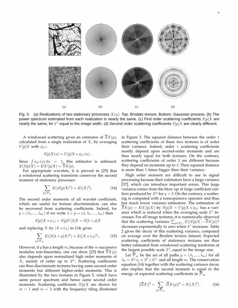
Image textures can be modeled as realizations of sta-tionary processes X(u). We denote the expected valueof X by E(X), which does not depend upon u. De-spite the importance of spectral methods, the powerspectrum is often not sufficient to discriminate imagetextures because it only depends upon second ordermoments. Figure 5 shows very different textures havingsame power spectrum. A scattering representation ofstationary processes depends upon second order andhigher-order moments, and can thus discriminate suchtextures. Moreover, it does not suffer from the largevariance curse of high order moments estimators [37],because it is computed with a nonexpansive operator.

If X(u) is stationary then U [p]X(u) remains stationarybecause it is computed with a cascade of convolutionsand modulus which preserve stationarity. Its expectedvalue thus does not depend upon u and defines theexpected scattering transform:

SX(p) = E(U [p]X) .

9

(a) (b) (c) (d)

Fig. 5. (a) Realizations of two stationary processes X(u). Top: Brodatz texture. Bottom: Gaussian process. (b) Thepower spectrum estimated from each realization is nearly the same. (c) First order scattering coefficients S[p]X arenearly the same, for 2J equal to the image width. (d) Second order scattering coefficients S[p]X are clearly different.

A windowed scattering gives an estimator of SX(p),calculated from a single realization of X , by averagingU [p]X with φ2J :

S[p]X(u) = U [p]X ⋆ φ2J (u) .

Since∫φ2J (u) du = 1, this estimator is unbiased:

E(S[p]X) = E(U [p]X) = SX(p).For appropriate wavelets, it is proved in [25] that

a windowed scattering transform conserves the secondmoment of stationary processes:

∑

p∈P∞

E(|S[p]X |2) = E(|X |2) . (14)

The second order moments of all wavelet coefficient,which are useful for texture discrimination, can alsobe recovered from scattering coefficients. Indeed, forp = (λ1, ..., λm) if we write λ+ p = (λ, λ1, ..., λm) then

S[p]|X ⋆ ψλ| = S[p]U [λ]X = S[λ+ p]X

and replacing X by |X ⋆ ψλ| in (14) gives∑

p∈P∞

E(|S[λ+ p]X |2) = E(|X ⋆ ψλ|2) . (15)

However, if p has a length m, because of the m successivemodulus non-linearities, one can show [25] that SX(p)also depends upon normalized high order moments ofX , mainly of order up to 2m. Scattering coefficientscan thus discriminate textures having same second-ordermoments but different higher-order moments. This isillustrated by the two textures in Figure 5, which havesame power spectrum and hence same second ordermoments. Scattering coefficients S[p]X are shown form = 1 and m = 2 with the frequency tiling illustrated

in Figure 3. The squared distance between the order 1scattering coefficients of these two textures is of ordertheir variance. Indeed, order 1 scattering coefficientsmostly depend upon second-order moments and arethus nearly equal for both textures. On the contrary,scattering coefficients of order 2 are different becausethey depend on moments up to 4. Their squared distanceis more than 5 times bigger than their variance.

High order moment are difficult to use in signalprocessing because their estimators have a large variance[37], which can introduce important errors. This largevariance comes from the blow up of large coefficient out-liers produced by Xq for q > 2. On the contrary, a scatter-ing is computed with a nonexpansive operator and thushas much lower variance estimators. The estimation ofSX(p) = E(U [p]X) by S[p]X = U [p]X ⋆ φ2J has a vari-ance which is reduced when the averaging scale 2J in-creases. For all image textures, it is numerically observedthat the scattering variance

∑p∈P∞

E(|S[p]X − SX(p)|2decreases exponentially to zero when 2J increases. Table2 gives the decay of this scattering variance, computedon average over the Brodatz texture dataset. Expectedscattering coefficients of stationary textures are thusbetter estimated from windowed scattering tranforms atthe largest possible scale 2J , equal to the image size.

Let P∞ be the set of all paths p = (λ1, ..., λm) for allλk = 2jkrk ∈ 2Z×G+ and all length m. The conservationequation (14) together with the scattering variance decayalso implies that the second moment is equal to theenergy of expected scattering coefficients in P∞

‖SX‖2 =∑

p∈P∞

|SX(p)|2 = E(|X |2) . (16)

10

TABLE 2Normalized scattering variance∑

p∈P∞E(|S[p]X − SX(p)|2)/E(|X |2), as a function of

J , computed on zero-mean and unit variance images ofthe Brodatz dataset, with cubic spline wavelets.

J = 1 J = 2 J = 3 J = 4 J = 5 J = 6 J = 7

0.85 0.65 0.45 0.26 0.14 0.07 0.0025

TABLE 3Percentage of energy

∑p∈Pm

↓|SX(p)|2/E(|X |2) along

frequency decreasing paths of length m, computed onthe normalized Brodatz dataset, with cubic spline

wavelets.

m = 0 m = 1 m = 2 m = 3 m = 4

0 74 19 3 0.3

Indeed E(S[p]X) = SX(p) so

E(|S[p]X |2) = SX(p)2 + E(|S[p]X − E(S[p]X)|2) .

Summing over p and letting J go to ∞ gives (16).Table 3 gives the ratio between the average energy

along frequency decreasing paths of length m and sec-ond moments, for textures in the Brodatz data set. Mostof this energy is concentrated over paths of length m ≤ 3.

3.4 Cosine Scattering Transform

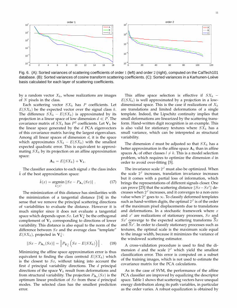
Natural images have scattering coefficients S[p]X(u)which are correlated across paths p = (λ1, ..., λm), at anygiven position u. The strongest correlation is betweencoefficients of a same layer. For each m, scattering coeffi-cients are decorrelated in a Karhunen-Loeve basis whichdiagonalizes their covariance matrix. Figure 6 comparesthe decay of the sorted variances E(|S[p]X−E(S[p]X)|2)and the variance decay in the Karhunen-Loeve basiscomputed over half of the Caltech image dataset, for thefirst layer and second coefficients. Scattering coefficientsare calculated with a Morlet wavelet. The variance decay(computed on the second half data set) is much faster inthe Karhunen-Loeve basis, which shows that there is astrong correlation between scattering coefficients of samelayers.

A change of variables proves that a rotation andscaling X2lr(u) = X(2−lru) produces a rotation andinverse scaling on the path variable

SX2lr(p) = SX(2lrp) where 2lrp = (2lrλ1, ..., 2lrλm) ,

and 2lrλk = 2l−jkrrk . If natural images can be con-sidered as randomly rotated and scaled [29], then thepath p is randomly rotated and scaled. In this case, thescattering transform has stationary variations along thescale and rotation variables. This suggests approximat-ing the Karhunen-Loeve basis by a cosine basis alongthese variables. Let us parametrize each rotation r by its

angle θ ∈ [0, 2π]. A path p = (2−j1r1, ..., 2−jkrk) is then

parametrized by ((j1, θ1), ..., (jm, θm)).Since scattering coefficients are computed along fre-

quency decreasing paths for which 0 < jk < jk+1 ≤ J ,to reduce boundary effects, a separable cosine transformis computed along the variables l1 = j1 , l2 = j2 −j1, ... , lm = jm − jm−1, and along each angle variableθ1, θ2, ... , θm. Cosine scattering coefficients are by ap-plying this separable discrete cosine transform along thescale and angle variables of S[p]X(u), for each u andeach path length m. Figure 6 shows that the cosinescattering coefficients have variances for m = 1 andm = 2 which decay nearly as fast as the variances inthe Karhunen-Loeve basis. It shows that a DCT acrossscales and orientations is nearly optimal to decorrelatescattering coefficients. Lower-frequency DCT coefficientsabsorb most of the scattering energy. On natural images,more than 99.5% of the scattering energy is absorbed bythe 1/2 lowest frequency cosine scattering coefficients.

We saw in (13) that without oversampling α = 1,when m = 2, an image of size N is represented byP = N 2−2J (KJ +K2J(J − 1)/2) scattering coefficients.Numerical computations are performed with K = 6 rota-tion angles and the DCT reduces at least by 2 the numberof coefficients. At a small invariant scale J = 2, theresulting cosine scattering representation has P = 3N/2coefficients. As a matter of comparison, SIFT representssmall blocks of 42 pixels with 8 coefficients, and a denseSIFT representation thus has N/2 coefficients. When Jincreases, the size of a cosine scattering representationdecreases like 2−2J , with P = N for J = 3 and P ≈ N/40for J = 7.

4 CLASSIFICATION

A scattering transform eliminates the image variabilitydue to translations and linearizes small deformations.Classification is studied with linear generative modelscomputed with a PCA, and with discriminant SVMclassifiers. State-of-the-art results are obtained for hand-written digit recognition and for texture discrimination.Scattering representations are computed with a Morletwavelet.

4.1 PCA Affine Space Selection

Although discriminant classifiers such as SVM havebetter asymptotic properties than generative classifiers[28], the situation can be inverted for small training sets.We introduce a simple robust generative classifier basedon affine space models computed with a PCA. Applyinga DCT on scattering coefficients has no effect on anylinear classifier because it is a linear orthogonal trans-form. Keeping the 50% lower frequency cosine scatteringcoefficients reduces computations and has a negligibleeffect on classification results. The classification algo-rithm is described directly on scattering coefficients tosimplify explanations. Each signal class is represented

11

0 2 4 6 8 10 12 14 16 1810

−3

10−2

10−1

100

101

102

order 1

ABC

0 20 40 60 80 100 12010

−6

10−4

10−2

100

102

order 2

ABC

Fig. 6. (A): Sorted variances of scattering coefficients of order 1 (left) and order 2 (right), computed on the CalTech101database. (B): Sorted variances of cosine transform scattering coefficients. (C): Sorted variances in a Karhunen-Loevebasis calculated for each layer of scattering coefficients.

by a random vector Xk, whose realizations are imagesof N pixels in the class.

Each scattering vector SXk has P coefficients. LetE(SXk) be the expected vector over the signal class k.The difference SXk − E(SXk) is approximated by itsprojection in a linear space of low dimension d≪ P . Thecovariance matrix of SXk has P 2 coefficients. Let Vk bethe linear space generated by the d PCA eigenvectorsof this covariance matrix having the largest eigenvalues.Among all linear spaces of dimension d, it is the spacewhich approximates SXk − E(SXk) with the smallestexpected quadratic error. This is equivalent to approxi-mating SXk by its projection on an affine approximationspace:

Ak = ESXk + Vk.

The classifier associates to each signal x the class indexk of the best approximation space:

k(x) = argmink≤C

‖Sx− PAk(Sx)‖ . (17)

The minimization of this distance has similarities withthe minimization of a tangential distance [14] in thesense that we remove the principal scattering directionsof variabilities to evaluate the distance. However it ismuch simpler since it does not evaluate a tangentialspace which depends upon Sx. Let V

⊥k be the orthogonal

complement of Vk corresponding to directions of lowervariability. This distance is also equal to the norm of thedifference between Sx and the average class “template”E(SXk), projected in V

⊥k :

‖Sx− PAk(Sx)‖ =

∥∥∥PV⊥k

(Sx− E(SXk)

)∥∥∥ . (18)

Minimizing the affine space approximation error is thusequivalent to finding the class centroid E(SXk) whichis the closest to Sx, without taking into account thefirst d principal variability directions. The d principaldirections of the space Vk result from deformations andfrom structural variability. The projection PAk

(Sx) is theoptimum linear prediction of Sx from these d principalmodes. The selected class has the smallest predictionerror.

This affine space selection is effective if SXk −E(SXk) is well approximated by a projection in a low-dimensional space. This is the case if realizations of Xk

are translations and limited deformations of a singletemplate. Indeed, the Lipschitz continuity implies thatsmall deformations are linearized by the scattering trans-form. Hand-written digit recognition is an example. Thisis also valid for stationary textures where SXk has asmall variance, which can be interpreted as structuralvariability.

The dimension d must be adjusted so that SXk has abetter approximation in the affine space Ak than in affinespaces Al of other classes l 6= k. This is a model selectionproblem, which requires to optimize the dimension d inorder to avoid over-fitting [5].

The invariance scale 2J must also be optimized. Whenthe scale 2J increases, translation invariance increasesbut it comes with a partial loss of information, whichbrings the representations of different signals closer. Onecan prove [25] that the scattering distance ‖Sx−Sx′‖ de-creases when 2J increases, and it converges to a non-zerovalue when 2J goes to ∞. To classify deformed templatessuch as hand-written digits, the optimal 2J is of the orderof the maximum pixel displacements due to translationsand deformations. In a stochastic framework where xand x′ are realizations of stationary processes, Sx andSx′ converge to the expected scattering transforms Sxand Sx′. In order to classify stationary processes such astextures, the optimal scale is the maximum scale equalto the image width, because it minimizes the variance ofthe windowed scattering estimator.

A cross-validation procedure is used to find the di-mension d and the scale 2J which yield the smallestclassification error. This error is computed on a subsetof the training images, which is not used to estimate thecovariance matrix for the PCA calculations.

As in the case of SVM, the performance of the affinePCA classifier are improved by equalizing the descriptorspace. Table 1 shows that scattering vectors have unequalenergy distribution along its path variables, in particularas the order varies. A robust equalization is obtained by

12

dividing each S[p]X(u) by

γ(p) = maxxi

( ∑

u

|S[p]xi(u)|2)1/2

, (19)

where the maximum is computed over all training sig-nals xi. To simplify notations, we still write SX the vec-tor of normalized scattering coefficients S[p]X(u)/γ(p).

Affine space scattering models can be interpreted asgenerative models computed independently for eachclass. As opposed to discriminative classifiers such asSVM, we do not estimate cross-correlation interactionsbetween classes, besides optimizing the model dimen-sion d. Such estimators are particularly effective forsmall number of training samples per class. Indeed, ifthere are few training samples per class then varianceterms dominate bias errors when estimating off-diagonalcovariance coefficients between classes [4].

An affine space approximation classifier can also beinterpreted as a robust quadratic discriminant classifierobtained by coarsely quantizing the eigenvalues of theinverse covariance matrix. For each class, the eigenval-ues of the inverse covariance are set to 0 in Vk and to1 in V

⊥k , where d is adjusted by cross-validation. This

coarse quantization is justified by the poor estimationof covariance eigenvalues from few training samples.These affine space models are robust when applied todistributions of scattering vectors having non-Gaussiandistributions, where a Gaussian Fisher discriminant canlead to significant errors.

4.2 Handwritten Digit Recognition

The MNIST database of hand-written digits is an exam-ple of structured pattern classification, where most ofthe intra-class variability is due to local translations anddeformations. It comprises at most 60000 training sam-ples and 10000 test samples. If the training dataset is notaugmented with deformations, the state of the art wasachieved by deep-learning convolution networks [31],deformation models [17], [3], and dictionary learning[27]. These results are improved by a scattering classifier.

All computations are performed on the reduced cosinescattering representation described in Section 3.4, whichkeeps the lower-frequency half of the coefficients. Table4 computes classification errors on a fixed set of testimages, depending upon the size of the training set,for different representations and classifiers. The affinespace selection of section 4.1 is compared with an SVMclassifier using RBF kernels, which are computed us-ing Libsvm [10], and whose variance is adjusted usingstandard cross-validation over a subset of the trainingset. The SVM classifier is trained with a renormalizationwhich maps all coefficients to [−1, 1]. The PCA classifieris trained with the renormalisation factors (19). The firsttwo columns of Table 4 show that classification errorsare much smaller with an SVM than with the PCAalgorithm if applied directly on the image. The 3rd and4th columns give the classification error obtained with

a PCA or an SVM classification applied to the modulusof a windowed Fourier transform. The spatial size 2J ofthe window is optimized with a cross-validation whichyields a minimum error for 2J = 8. It correspondsto the largest pixel displacements due to translationsor deformations in each class. Removing the complexphase of the windowed Fourier transform yields a locallyinvariant representation but whose high frequencies areunstable to deformations, as explained in Section 2.1.Suppressing this local translation variability improvesthe classification rate by a factor 3 for a PCA and byalmost 2 for an SVM. The comparison between PCAand SVM confirms the fact that generative classifierscan outperform discriminative classifiers when trainingsamples are scarce [28]. As the training set size increases,the bias-variance trade-off turns in favor of the richerSVM classifiers, independently of the descriptor.

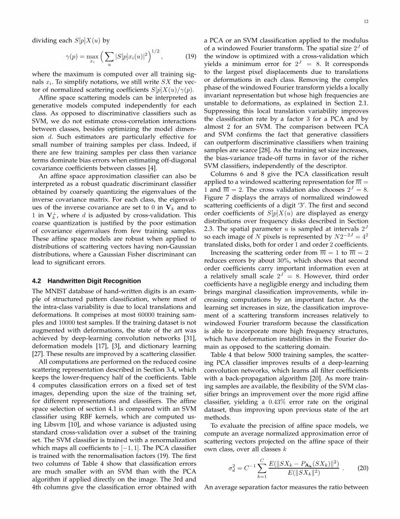
Columns 6 and 8 give the PCA classification resultapplied to a windowed scattering representation for m =1 and m = 2. The cross validation also chooses 2J = 8.Figure 7 displays the arrays of normalized windowedscattering coefficients of a digit ‘3’. The first and secondorder coefficients of S[p]X(u) are displayed as energydistributions over frequency disks described in Section2.3. The spatial parameter u is sampled at intervals 2J

so each image of N pixels is represented by N2−2J = 42

translated disks, both for order 1 and order 2 coefficients.Increasing the scattering order from m = 1 to m = 2

reduces errors by about 30%, which shows that secondorder coefficients carry important information even ata relatively small scale 2J = 8. However, third ordercoefficients have a negligible energy and including thembrings marginal classification improvements, while in-creasing computations by an important factor. As thelearning set increases in size, the classification improve-ment of a scattering transform increases relatively towindowed Fourier transform because the classificationis able to incorporate more high frequency structures,which have deformation instabilities in the Fourier do-main as opposed to the scattering domain.

Table 4 that below 5000 training samples, the scatter-ing PCA classifier improves results of a deep-learningconvolution networks, which learns all filter coefficientswith a back-propagation algorithm [20]. As more train-ing samples are available, the flexibility of the SVM clas-sifier brings an improvement over the more rigid affineclassifier, yielding a 0.43% error rate on the originaldataset, thus improving upon previous state of the artmethods.

To evaluate the precision of affine space models, wecompute an average normalized approximation error ofscattering vectors projected on the affine space of theirown class, over all classes k

σ2d = C−1

C∑

k=1

E(‖SXk − PAk(SXk)‖2)

E(‖SXk‖2). (20)

An average separation factor measures the ratio between

13

(a) (b) (c)

Fig. 7. (a): Image X(u) of a digit ’3’. (b): Arrays of windowed scattering coefficients S[p]X(u) of order m = 1, with usampled at intervals of 2J = 8 pixels. (c): Windowed scattering coefficients S[p]X(u) of order m = 2.

TABLE 4Percentage of errors of MNIST classifiers, depending on the training size.

Training x Wind. Four. Scat. m = 1 Scat. m = 2 Conv.size PCA SVM PCA SVM PCA SVM PCA SVM Net.300 14.5 15.4 7.35 7.4 5.7 8 4.7 5.6 7.18

1000 7.2 8.2 3.74 3.74 2.35 4 2.3 2.6 3.212000 5.8 6.5 2.99 2.9 1.7 2.6 1.3 1.8 2.535000 4.9 4 2.34 2.2 1.6 1.6 1.03 1.4 1.5210000 4.55 3.11 2.24 1.65 1.5 1.23 0.88 1 0.85

20000 4.25 2.2 1.92 1.15 1.4 0.96 0.79 0.58 0.7640000 4.1 1.7 1.85 0.9 1.36 0.75 0.74 0.53 0.6560000 4.3 1.4 1.80 0.8 1.34 0.62 0.7 0.43 0.53

TABLE 5For each MNIST training size, the table gives the

cross-validated dimension d of affine approximationspaces, together with the average approximation error σ2

d

and separation ratio ρ2d of these spaces.

Training d σ2

dρ2

d

300 5 3 · 10−1 2

5000 100 4 · 10−2 3

40000 140 2 · 10−2 4

the approximation error in the affine space Ak of thesignal class and the minimum approximation error inanother affine model Al with l 6= k, for all classes k

ρ2d = C−1

C∑

k=1

E(minl 6=k ‖SXk − PAl(SXk)‖2)

E(‖SXk − PAk(SXk)‖2)

. (21)

For a scattering representation with m = 2, Table 5gives the dimension d of affine approximation spacesoptimized with a cross validation. It varies considerably,ranging from 5 to 140 when the number of trainingexamples goes from 300 to 40000. Indeed, many trainingsamples are needed to estimate reliably the eigenvectorsof the covariance matrix and thus to compute reliableaffine space models for each class. The average ap-proximation error σ2

d of affine space models is progres-sively reduced while the separation ratio ρ2

d increases.It explains the reduction of the classification error rateobserved in Table 4, as the training size increases.

TABLE 6Percentage of errors for the whole USPS database.

Tang. Scat. m = 2 Scat. m = 1 Scat. m = 2

Kern. SVM PCA PCA2.4 2.7 3.24 2.6 / 2.3

The US-Postal Service is another handwritten digitdataset, with 7291 training samples and 2007 test images16×16 pixels. The state of the art is obtained with tangentdistance kernels [14]. Table 6 gives results obtainedwith a scattering transform with the PCA classifier form = 1, 2. The cross-validation sets the scattering scale to2J = 8. As in the MNIST case, the error is reduced whengoing from m = 1 to m = 2 but remains stable for m = 3.Different renormalization strategies can bring marginalimprovements on this dataset. If the renormalization isperformed by equalizing using the standard deviation ofeach component, the classification error is 2.3% whereasit is 2.6% if the supremum is normalized.

The scattering transform is stable but not invariantto rotations. Stability to rotations is demonstrated overthe MNIST database in the setting defined in [18]. Adatabase with 12000 training samples and 50000 testimages is constructed with random rotations of MNISTdigits. The PCA affine space selection takes into accountthe rotation variability by increasing the dimension dof the affine approximation space. This is equivalentto projecting the distance to the class centroid on asmaller orthogonal space, by removing more principal

14

TABLE 7Percentage of errors on an MNIST rotated dataset [18].

Scat. m = 1 Scat. m = 2 Conv.PCA PCA Net.

8 4.4 8.8

TABLE 8Percentage of errors on scaled/rotated MNIST digits

Transformations Scat. m = 1 Scat. m = 2

on MNIST images PCA PCANone 1.6 0.8

Rotations 6.7 3.3Scalings 2 1

Rot. + Scal. 12 5.5

components. The error rate in Table 7 is much smallerwith a scattering PCA than with a convolution network[18]. Much better results are obtained for a scatteringwith m = 2 than with m = 1 because second ordercoefficients maintain enough discriminability despite theremoval of a larger number d of principal directions. Inthis case, m = 3 marginally reduces the error.

Scaling and rotation invariance is studied by intro-ducing a random scaling factor uniformly distributedbetween 1/

√2 and

√2, and a random rotation by a uni-

form angle. In this case, the digit ‘9’ is removed from thedatabase as to avoid any indetermination with the digit‘6’ when rotated. The training set has 9000 samples (1000samples per class). Table 8 gives the error rate on theoriginal MNIST database when transforming the trainingand testing samples either with random rotations, scal-ings, or both. Scalings have a smaller impact on the errorrate than rotations because scaled scattering vectors spanan invariant linear space of lower dimension. Second-order scattering outperforms first-order scattering, andthe difference becomes more significant when rotationand scaling are combined. Second order coefficients arehighly discriminative in presence of scaling and rotationvariability.

4.3 Texture Discrimination

Visual texture discrimination remains an outstandingimage processing problem because textures are realiza-tions of non-Gaussian stationary processes, which cannotbe discriminated using the power spectrum. The affinePCA space classifier removes most of the variability ofSX − ESX within each class. This variability is dueto the residual stochastic variability which decays as Jincreases, and to variability due to illumination, rotation,scaling, or perspective deformations when textures aremapped on surfaces.

Texture classification is tested on the CUReT texturedatabase [21], [36], which includes 61 classes of imagetextures of N = 2002 pixels. Each texture class givesimages of the same material with different pose and

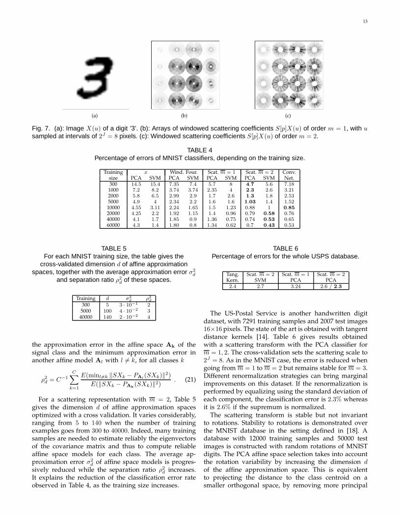
illumination conditions. Specularities, shadowing andsurface normal variations make classification challeng-ing. Pose variation requires global rotation and illumi-nation invariance. Figure 8 illustrates the large intra-class variability, after a normalization of the mean andvariance of each textured image.

Table 9 compares error rates obtained with differentimage representations. The database is randomly splitinto a training and a testing set, with 46 training imagesfor each class as in [36]. Results are averaged over 10different splits. A PCA affine space classifier applieddirectly on the image pixels yields a large classificationerror of 17%. The lowest published classification errorsobtained on this dataset are 2% for Markov RandomFields [36], 1.53% for a dictionary of textons [15], 1.4%for Basic Image Features [11] and 1% for histogramsof image variations [6]. A PCA classifier applied toa Fourier power spectrum estimator also reaches 1%error. The power spectrum is estimated with windowedFourier transforms calculated over half-overlapping win-dows, whose squared modulus are averaged over thewhole image to reduce the estimator variance. A cross-validation optimizes the window size to 2J = 32 pixels.

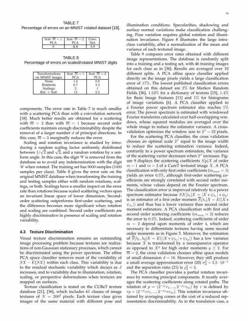
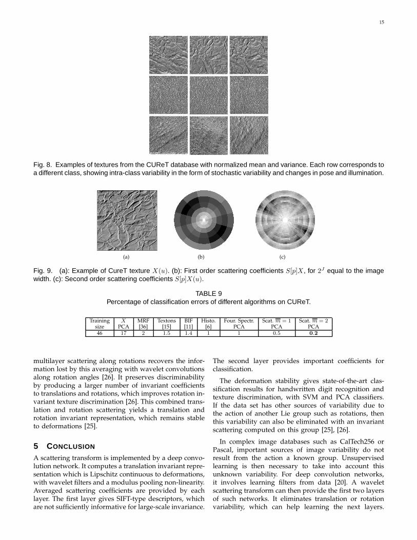
For the scattering PCA classifier, the cross validationchooses an optimal scale 2J equal to the image widthto reduce the scattering estimation variance. Indeed,contrarily to a power spectrum estimation, the varianceof the scattering vector decreases when 2J increases. Fig-ure 9 displays the scattering coefficients S[p]X of orderm = 1 and m = 2 of a CureT textured image X . A PCAclassification with only first order coefficients (mmax = 1)yields an error 0.5%, although first-order scattering co-efficients are strongly correlated with second order mo-ments, whose values depend on the Fourier spectrum.The classification error is improved relatively to a powerspectrum estimator because SX [λ1]X = |X ⋆ ψλ1

| ⋆ φ2J

is an estimator of a first order moment S[λ1]X = E(|X ⋆ψλ1

|) and thus has a lower variance than second ordermoment estimators. A PCA classification with first andsecond order scattering coefficients (mmax = 2) reducesthe error to 0.2%. Indeed, scattering coefficients of orderm = 2 depend upon moments of order 4, which arenecessary to differentiate textures having same secondorder moments as in Figure 5. Moreover, the estimationof S[λ1, λ2]X = E(||X ⋆ ψλ1

| ⋆ ψλ2|) has a low variance

because X is transformed by a nonexpansive operatoras opposed to Xq for high order moments q ≥ 2. Form = 2, the cross validation chooses affine space modelsof small dimension d = 16. However, they still producea small average approximation error (20) σ2

d = 2.5 · 10−1

and the separation ratio (21) is ρ2d = 3.

The PCA classifier provides a partial rotation invari-ance by removing principal components. It mostly aver-ages the scattering coefficients along rotated paths. Therotation of p = (2−j1r1, ..., 2

−jmrm) by r is defined byrp = (2−j1rr1, ..., 2

−jmrrm). This rotation invariance ob-tained by averaging comes at the cost of a reduced rep-resentation discriminability. As in the translation case, a

15

Fig. 8. Examples of textures from the CUReT database with normalized mean and variance. Each row corresponds toa different class, showing intra-class variability in the form of stochastic variability and changes in pose and illumination.

(a) (b) (c)

Fig. 9. (a): Example of CureT texture X(u). (b): First order scattering coefficients S[p]X , for 2J equal to the imagewidth. (c): Second order scattering coefficients S[p]X(u).

TABLE 9Percentage of classification errors of different algorithms on CUReT.

Training X MRF Textons BIF Histo. Four. Spectr. Scat. m = 1 Scat. m = 2

size PCA [36] [15] [11] [6] PCA PCA PCA46 17 2 1.5 1.4 1 1 0.5 0.2

multilayer scattering along rotations recovers the infor-mation lost by this averaging with wavelet convolutionsalong rotation angles [26]. It preserves discriminabilityby producing a larger number of invariant coefficientsto translations and rotations, which improves rotation in-variant texture discrimination [26]. This combined trans-lation and rotation scattering yields a translation androtation invariant representation, which remains stableto deformations [25].

5 CONCLUSION

A scattering transform is implemented by a deep convo-lution network. It computes a translation invariant repre-sentation which is Lipschitz continuous to deformations,with wavelet filters and a modulus pooling non-linearity.Averaged scattering coefficients are provided by eachlayer. The first layer gives SIFT-type descriptors, whichare not sufficiently informative for large-scale invariance.

The second layer provides important coefficients forclassification.

The deformation stability gives state-of-the-art clas-sification results for handwritten digit recognition andtexture discrimination, with SVM and PCA classifiers.If the data set has other sources of variability due tothe action of another Lie group such as rotations, thenthis variability can also be eliminated with an invariantscattering computed on this group [25], [26].

In complex image databases such as CalTech256 orPascal, important sources of image variability do notresult from the action a known group. Unsupervisedlearning is then necessary to take into account thisunknown variability. For deep convolution networks,it involves learning filters from data [20]. A waveletscattering transform can then provide the first two layersof such networks. It eliminates translation or rotationvariability, which can help learning the next layers.

16

Similarly, scattering coefficients can replace SIFT vectorsfor bag-of-feature clustering algorithms [8]. Indeed, weshowed that second layer scattering coefficients pro-vide important complementary information, with a smallcomputational and memory cost.

REFERENCES

[1] S. Allassonniere, Y. Amit, A. Trouve, “Toward a coherent statisticalframework for dense deformable template estimation”. Volume69, part 1 (2007), pages 3-29, of the Journal of the Royal StatisticalSociety.

[2] J. Anden, S. Mallat, “Scattering audio representations”, subm. toIEEE Trans. on IEEE Trans. on Signal Processing.

[3] Y. Amit, A. Trouve, “POP. Patchwork of Parts Models for ObjectRecognition”, ICJV Vol 75, 2007.

[4] P. J. Bickel and E. Levina: “Covariance regularization by thresh-olding”, Annals of Statistics, 2008.

[5] L. Birge and P. Massart. “From model selection to adaptiveestimation.” In Festschrift for Lucien Le Cam: Research Papersin Probability and Statistics, 55 - 88, Springer-Verlag, New York,1997.

[6] R. E. Broadhurst, “Statistical estimation of histogram variation fortexture classification,” in Proc. Workshop on Texture Analysis andSynthesis, Beijing 2005.

[7] J. Bruna, “Scattering representations for pattern and texture recog-nition”, Ph.D thesis, CMAP, Ecole Polytechnique, 2012.

[8] Y-L. Boureau, F. Bach, Y. LeCun, and J. Ponce. “Learning Mid-Level Features For Recognition”. In IEEE Conference on Com-puter Vision and Pattern Recognition, 2010.

[9] J. Bouvrie, L. Rosasco, T. Poggio: “On Invariance in HierarchicalModels”, NIPS 2009.

[10] C. Chang and C. Lin, “LIBSVM : a library for support vectormachines”. ACM Transactions on Intelligent Systems and Tech-nology, 2:27:1–27:27, 2011.

[11] M. Crosier and L. Griffin, “Using Basic Image Features for TextureClassification”, Int. Jour. of Computer Vision, pp. 447-460, 2010.

[12] L. Fei-Fei, R. Fergus and P. Perona. “Learning generative visualmodels from few training examples: an incremental Bayesianapproach tested on 101 object categories”. IEEE. CVPR 2004

[13] Z. Guo, L. Zhang, D. Zhang, “Rotation Invariant texture classifi-cation using LBP variance (LBPV) with global matching”, ElsevierJournal of Pattern Recognition, Aug. 2009.

[14] B.Haasdonk, D.Keysers: “Tangent Distance kernels for supportvector machines”, 2002.

[15] E. Hayman, B. Caputo, M. Fritz and J.O. Eklundh, “On theSignificance of Real-World Conditions for Material Classification”,ECCV, 2004.

[16] K. Jarrett, K. Kavukcuoglu, M. Ranzato and Y. LeCun: “What isthe Best Multi-Stage Architecture for Object Recognition?”, Proc.of ICCV 2009.

[17] D.Keysers, T.Deselaers, C.Gollan, H.Ney, “Deformation Modelsfor image recognition”, IEEE trans of PAMI, 2007.

[18] H. Larochelle, Y. Bengio, J. Louradour, P. Lamblin, “ExploringStrategies for Training Deep Neural Networks”, Journal of Ma-chine Learning Research, Jan. 2009.

[19] S. Lazebnik, C. Schmid, J.Ponce. “Beyond Bags of Features: SpatialPyramid Matching for Recognizing Natural Scene Categories”,CVPR 2006.

[20] Y. LeCun, K. Kavukvuoglu and C. Farabet: “Convolutional Net-works and Applications in Vision”, Proc. of ISCAS 2010.

[21] T. Leung and J. Malik; “Representing and Recognizing the VisualAppearance of Materials Using Three-Dimensional Textons”. In-ternational Journal of Computer Vision, 43(1), 29-44; 2001.

[22] J. Lindenstrauss, D. Preiss, J. Tise, “Frechet Differentiability ofLipschitz Functions and Porous Sets in Banach Spaces”, PrincetonUniv. Press, 2012.

[23] D.G. Lowe, “Distinctive Image Features from Scale-Invariant Key-points”, International Journal of Computer Vision, 60, 2, pp. 91-110, 2004

[24] S. Mallat, “Recursive Interferometric Representation”, Proc. ofEUSIPCO, Denmark, August 2010.

[25] S. Mallat “Group Invariant Scattering”, Communications in Pureand Applied Mathematics, vol. 65, no. 10. pp. 1331-1398, October2012.

[26] L. Sifre, S. Mallat, “Combined scattering for rotation invarianttexture analysis”, Proc. of ESANN, April 2012.

[27] J. Mairal, F. Bach, J.Ponce, “Task-Driven Dictionary Learning”,Submitted to IEEE trans. on PAMI, September 2010.

[28] A. Y. Ng and M. I. Jordan “On discriminative vs. generativeclassifiers: A comparison of logistic regression and naive Bayes”,in Advances in Neural Information Processing Systems (NIPS) 14,2002.

[29] L. Perrinet, “Role of Homeostasis in Learning Sparse Representa-tions”, Neural Computation Journal, 2010.

[30] J.Portilla, E.Simoncelli, “A Parametric Texture model based onjoint statistics of complex wavelet coefficients”, IJCV, 2000.

[31] M. Ranzato, F.Huang, Y.Boreau, Y. LeCun: “Unsupervised Learn-ing of Invariant Feature Hierarchies with Applications to ObjectRecognition”, CVPR 2007.

[32] C. Sagiv, N. A. Sochen and Y. Y. Zeevi, ”Gabor Feature SpaceDiffusion via the Minimal Weighted Area Method”, SpringerLecture Notes in Computer Science, Vol. 2134, pp. 621-635, 2001.

[33] B. Scholkopf and A. J. Smola, “Learning with Kernels”, MIT Press,2002.

[34] S.Soatto, “Actionable Information in Vision”, ICCV, 2009.[35] E. Tola, V.Lepetit, P. Fua, “DAISY: An Efficient Dense Descriptor

Applied to Wide-Baseline Stereo”, IEEE trans on PAMI, May 2010.[36] M. Varma, A. Zisserman, “Texture classification: are filter banks

necessary?,” CVPR 2003.[37] M. Welling, “Robust Higher Order Statistics”, AISTATS 2005.[38] I. Waldspurger, S. Mallat “Recovering the phase of a complex

wavelet transform”, CMAP Tech. Report, Ecole Polytechnique,2012.

Joan Bruna Joan Bruna graduated from Univer-sitat Politecnica de Catalunya in both Mathemat-ics and Electrical Engineering, in 2002 and 2004respectively. He obtained an MSc in appliedmathematics from ENS Cachan in 2005. From2005 to 2010, he was a research engineer in animage processing startup, developing realtimevideo processing algorithms. He is currently pur-suing his PhD degree in Applied Mathematics atEcole Polytechnique, Palaiseau. His research in-terests include invariant signal representations,

stochastic processes and functional analysis.

Stephane Mallat Stephane Mallat received anengineering degree from Ecole Polytechnique,Paris, a Ph.D. in electrical engineering fromthe University of Pennsylvania, Philadelphia, in1988, and an habilitation in applied mathematicsfrom Universite Paris-Dauphine.

In 1988, he joined the Computer Science De-partment of the Courant Institue of MathematicalSciences where he was Associate Professor in1994 and Professsor in 1996. From 1995 to2012, he was a full Professor in the Applied

Mathematics Department at Ecole Polytechnique, Paris. From 2001 to2008 he was a co-founder and CEO of a start-up company. Since2012, he joined the computer science department of Ecole NormaleSuperieure, in Paris.

Dr. Mallat is an IEEE and EURASIP fellow. He received the 1990IEEE Signal Processing Society’s paper award, the 1993 Alfred Sloanfellowship in Mathematics, the 1997 Outstanding Achievement Awardfrom the SPIE Optical Engineering Society, the 1997 Blaise Pascal Prizein applied mathematics from the French Academy of Sciences, the 2004European IST Grand prize, the 2004 INIST-CNRS prize for most citedFrench researcher in engineering and computer science, and the 2007EADS prize of the French Academy of Sciences.

His research interests include computer vision, signal processing andharmonic analysis.