Inﬂuence of thermodynamic soil and vegetation ... · PDF fileInﬂuence of thermodynamic soil and vegetation parameterizations on the simulation of soil temperature states ... Experiment

Hydrol. Earth Syst. Sci., 13, 759–777, 2009www.hydrol-earth-syst-sci.net/13/759/2009/© Author(s) 2009. This work is distributed underthe Creative Commons Attribution 3.0 License.

Hydrology andEarth System

Sciences

Influence of thermodynamic soil and vegetation parameterizationson the simulation of soil temperature states and surface fluxes by theNoah LSM over a Tibetan plateau site

R. van der Velde1, Z. Su1, M. Ek2, M. Rodell3, and Y. Ma4

1International Institute for Geo-Information Science and Earth Observation (ITC), Hengelosestraat 99, P.O. Box 6, 7500 AAEnschede, The Netherlands2Environmental Modeling Center, National Center for Environmental Prediction, Suitland, Maryland, USA3Hydrological Science Branch, Code 614.3, NASA, Goddard Space Flight Center, Greenbelt, Maryland, USA4Institute of Tibetan Plateau Research (ITP/CAS), P.O. Box 2871, Beijing 100085, China

Received: 21 November 2008 – Published in Hydrol. Earth Syst. Sci. Discuss.: 21 January 2009Revised: 8 May 2009 – Accepted: 22 May 2009 – Published: 12 June 2009

Abstract. In this paper, we investigate the ability of the NoahLand Surface Model (LSM) to simulate temperature states inthe soil profile and surface fluxes measured during a 7-daydry period at a micrometeorological station on the TibetanPlateau. Adjustments in soil and vegetation parameteriza-tions required to ameliorate the Noah simulation on these twoaspects are presented, which include: (1) differentiating thesoil thermal properties of top- and subsoils, (2) investigationof the different numerical soil discretizations and (3) calibra-tion of the parameters utilized to describe the transpirationdynamics of the Plateau vegetation. Through the adjustmentsin the parameterization of the soil thermal properties (STP)simulation of the soil heat transfer is improved, which resultsin a reduction of Root Mean Squared Differences (RMSD’s)by 14%, 18% and 49% between measured and simulatedskin, 5-cm and 25-cm soil temperatures, respectively. Fur-ther, decreasing the minimum stomatal resistance (Rc,min)and the optimum temperature for transpiration (Topt) of thevegetation parameterization reduces RMSD’s between mea-sured and simulated energy balance components by 30%,20% and 5% for the sensible, latent and soil heat flux, re-spectively.

Correspondence to:R. van der Velde([email protected])

1 Introduction

An accurate characterization of the heat and moisture ex-change between the land surface and atmosphere is impor-tant for Atmospheric General Circulation Models (AGCM)to forecast weather at various time scales (i.e. McCumber andPielke, 1981; Garratt, 1993; Koster et al., 2004). Within op-erational AGCM these land-atmosphere interactions are de-scribed by a Land Surface Model (LSM). Because AGCMare computationally demanding, numerical efficiency of theLSM is required. Therefore, a simplified implementation ofthe physical processes and the applied parameterizations areinevitable. For example, the impact of a physically based for-mulation of roughness lengths for momentum and heat trans-port on the calculation of the surface fluxes has been stressed(i.e. Chen et al., 1997; Zeng and Dickinson, 1998; Su et al.,2001; Liu et al., 2007; Ma et al., 2008) and the influenceof a more detailed description of the land surface hydrologyhas been discussed (i.e. Gutmann and Small, 2007; Gulden etal., 2007). Furthermore, a limited number of soil and vege-tation parameterizations are accommodated in modeling sys-tems operational at a global scale (e.g. Ek et al., 2003).

The impact of those (and other) uncertainties in the sim-ulation of land processes on the output of an AGCM wasevaluated by Dickinson et al. (2006). They found signifi-cant differences between measured and simulated precipita-tion amounts and air temperatures for selected extreme en-vironments, such as the Sahara desert, the semi-arid Sahel,Amazonian rain forest and Tibetan Plateau. These findingsare supported by the results presented in Hogue et al. (2005),

Published by Copernicus Publications on behalf of the European Geosciences Union.

http://creativecommons.org/licenses/by/3.0/

760 R. van der Velde et al.: Simulation of surface processes over a Tibetan plateau site

which showed that thorough optimization of a comprehen-sive set of model parameters, can reduce differences be-tween the measured and simulated heat fluxes for the semi-arid Walnut Gulch watershed (Arizona, USA) by as much as20–40 W m−2. The investigation by Dickinson et al. (2006)demonstrates the existence of inconsistencies in the simula-tions of land surface processes, while Hogue et al. (2005)show that through adjustment of the LSM parameterizationsan improvement is obtained in the model’s performance.This suggests that even for extreme environment the imple-mented LSM physics is flexible enough to represent the landsurface processes adequately given the appropriate parame-terization.

Within the framework of the Model Parameter EstimationExperiment (MOPEX) the development of area specific landsurface parameterization has been accommodated (Schaakeet al., 2006). The focus of this initiative has been on the de-velopment parameter estimation methodologies and the cali-bration of parameters that affect primarily the rainfall-runoffrelationships (Duan et al., 2006). As a result, the influenceof model parameters on simulation of surface energy bal-ance has received little attention within MOPEX. One of thefew investigations that addressed the impact parameter un-certainty on energy balance simulations has been reported byKahan et al. (2006). They showed for the Simplified SimpleBiosphere (SSiB, Xue et al., 1991) model that adjustmentin the Leaf Area Index (LAI), stomatal resistance and satu-rated hydraulic conductivity (Ksat) are required to decreasesystematic differences between simulated and measured sen-sible and latent heat fluxes for a Sahelian study area in Niger.Moreover, the importance of proper thermal diffusivity isemphasized in order to reduce uncertainties in the simulateddiurnal evolution of the surface temperature and sensible heatflux. In a MOPEX-related study, Yang et al. (2005) haveshown for the Tibetan Plateau that also the vertical soil het-erogeneity may have a significant impact on the partitioningof radiation.

These previous investigations demonstrate that adjust-ments in soil and vegetation parameterizations can yield sig-nificant improvements in the simulation of the surface en-ergy balance. They also emphasize the need to analyze pa-rameter uncertainties of different LSM’s in more detail. Inthis context, the Noah LSM is employed to simulate the landsurface process of a Tibetan Plateau site for a 7-day dry pe-riod (3 September to 10 September 2005) during the AsianMonsoon. The objective of this study is to identify the ad-justments in soil and vegetation parameterizations needed toreconstruct the temperature states in the soil profile and themeasured surface energy fluxes over this short period. In thispaper, firstly, the results of Noah simulations obtained by us-ing standard parameterizations employed for application atglobal scales are presented. Secondly, the adjustments in thesoil and vegetation parameterizations are explored to opti-mize the model performance.

2 Data set

2.1 Study site

The study site selected for this investigation is themicro-meteorological Naqu station located (31.3686◦ N,91.8987◦ E) approximately 25 km southwest of Naqu city.This station is part of the meso-scale observational networkpreviously installed in the Naqu river basin in the frameworkof the GAME (GEWEX (Global Energy and Water cycle Ex-periment) Asian Monsoon Experiment) and CAMP (CEOP(Coordinated Enhanced Observing Period) Asia-AustraliaMonsoon Project) Tibet field campaigns. The heat flux mea-surements collected during these field campaigns have beenextensively used to improve the understanding on the wa-ter and energy exchange between the land surface and atmo-sphere over the Tibetan Plateau (e.g. Ma et al., 2002, 2005;Yang et al., 2005, 2008).

In Fig. 1 a subset of a LandSat TM false color imageis shown covering a part of the watershed and indicatingthe location of the study site. Despite the high overall al-titude (4500 m) and significant relief in some parts of thisregion, the terrain in the proximity of the study site is rela-tively smooth, varying only tens of meters in elevation. Theweather on this part of the plateau is influenced by the warmwet monsoon in the summer and cold dry winters with tem-peratures below freezing point. Land cover consists of shortprairie grasses in higher parts of the watershed and short wet-land vegetation in the local depressions. The direct environ-ment of Naqu station consists of short grasses, but withina hundred meters a wetland is situated. Based on textu-ral and hydraulic characterizations performed in the labo-ratory, the soils can be classified as sandy loam (70% sandand 10% silt) with a high saturated hydraulic conductivity(Ksat=1.2 m d−1) on top of an impermeable rock formation.Due to the high root density from the short grasses, organicmatter content in the top-soils is relatively high (14.2%).

At Naqu station, instrumentation has been installed tomeasure atmospheric variables at different levels (e.g. windspeed, humidity and temperature), incoming and outgoing(shortwave and longwave) radiation, turbulent heat fluxes,soil moisture at depths of 5 and 20 cm, and temperaturesin the soil profile up to a depth of 40 cm. All variablesare recorded at 10-min intervals and a list of the variablesused, here, is given in Table 1. From the data record ofNaqu station only a 7-day period from 3 to 10 September2005 has been selected for this investigation. This short pe-riod has been selected because the measured rainfall amountswere found to be unreliable due to mechanical difficultieswith the logging system and the tipping mechanism of therain gauge. Since rainfall is such a crucial forcing variable,the period between 3 and 10 September 2005 is used; be-ing the longest summer period without precipitation basedon available soil moisture and incoming shortwave radiationmeasurements. Although the selected period is identified as

Hydrol. Earth Syst. Sci., 13, 759–777, 2009 www.hydrol-earth-syst-sci.net/13/759/2009/

R. van der Velde et al.: Simulation of surface processes over a Tibetan plateau site 761

30

Figures:

Fig. 1: LandSat TM false color image acquired over the Tibetan study site and its approximate

location within the Tibetan Plateau. Fig. 1. LandSat TM false color image acquired over the Tibetan study site and its approximate location within the Tibetan Plateau.

completely dry, the soil moisture measurements indicate thatprior to 3 September several intensive rain events wetted theland surface. The selected period represents, thus, a typicaldry-down cycle, which is, in general, a solid basis for valida-tion of LSM parameterizations.

2.2 Surface fluxes

The soil heat flux is reconstructed using Fourier’s Lawfrom temperature gradient measurements between the sur-face (Tskin) and the soil depth at which the first temperaturemeasurements are made, which is 0.05 m (T5cm). This tem-perature gradient andG0 are related to each other as follows,

G0 = κh (sm)∂T

∂z= κh (sm)

Tskin − Ts1

dz(1)

whereκh is the thermal conductivity [W m−1 K−1], smis soilmoisture content [m3 m−3], z is the soil depth. Applicationof this approach requires formulation of the thermal conduc-tivity, which depends on the soil constituents, such as quartzand organic matter contents. Various scientists (e.g. de Vries,1963; Johansen, 1975; Peters-Lidard et al., 1998) have de-veloped generic formulations to relate the soil texture to thethermal conductivity. In Hillel (1998), however, it is pointedout thatκh not merely depends on the soil constituents, butis also affected by the size, shape and spatial arrangementof soil particles. Given the rather specific conditions on theTibetan Plateau,κh under the initial soil moisture conditions

(κ ih) of the analyzed period is derived from the measured soilheat flux at a soil depth of 10 cm (G10) and the soil tempera-ture gradient. Using theκ ih, theκh is extrapolated for follow-ing time steps using the measured soil moisture accordingto,

κh (sm) = κ ih + (smi − sm) κw (2)

where, κw is the thermal conductivity of water[=0.57 W m−1 K−1], and sub- and superscripti refer tothe initial conditions of the selected period.

Unfortunately, the turbulent heat fluxes measured by theeddy correlation (EC) instrumentation at Naqu station are notavailable for the selected period. Therefore, the sensible (H )and latent heat (λE) fluxes have been computed using theBowen Ratio Energy Balance (BREB)– method (i.e. Perez etal., 1999; Pauwels and Samson, 2006), whereby the BowenRatio (β) is defined as,

β =H

λE= γ

Tair1 − Tair2

eair1 − eair2(3)

where,e is vapor pressure [kPa], subscripts air1 and air2 in-dicate the first and second atmospheric level, respectively,andγ is psychrometric constant [kPa K−1] defined as,

γ =cpP

0.622· λ(4)

where, cp is specific heat capacity of moist air[=1005 kJ kg−1 K1], P is the air pressure [kPa] andλis the latent heat of vaporization [=2.5·106 J kg−1].

www.hydrol-earth-syst-sci.net/13/759/2009/ Hydrol. Earth Syst. Sci., 13, 759–777, 2009


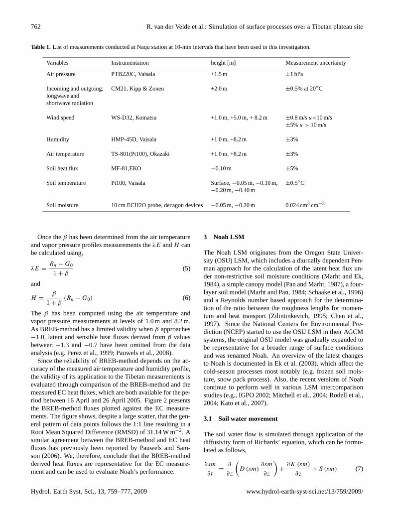
Table 1. List of measurements conducted at Naqu station at 10-min intervals that have been used in this investigation.

Variables Instrumentation height [m] Measurement uncertainty

Air pressure PTB220C, Vaisala +1.5 m ±1 hPa

Incoming and outgoing, CM21, Kipp & Zonen +2.0 m ±0.5% at 20◦Clongwave andshortwave radiation

Wind speed WS-D32, Komatsu +1.0 m, +5.0 m, + 8.2 m ±0.8 m/su<10 m/s±5%u > 10 m/s

Humidity HMP-45D, Vaisala +1.0 m, +8.2 m ±3%

Air temperature TS-801(Pt100), Okazaki +1.0 m, +8.2 m ±3%

Soil heat flux MF-81,EKO −0.10 m ±5%

Soil temperature Pt100, Vaisala Surface,−0.05 m,−0.10 m, ±0.5◦C−0.20 m,−0.40 m

Soil moisture 10 cm ECH2O probe, decagon devices−0.05 m,−0.20 m 0.024 cm3 cm−3

Once theβ has been determined from the air temperatureand vapor pressure profiles measurements theλE andH canbe calculated using,

λE =Rn −G0

1 + β(5)

and

H =β

1 + β(Rn −G0) (6)

The β has been computed using the air temperature andvapor pressure measurements at levels of 1.0 m and 8.2 m.As BREB-method has a limited validity whenβ approaches−1.0, latent and sensible heat fluxes derived fromβ valuesbetween−1.3 and−0.7 have been omitted from the dataanalysis (e.g. Perez et al., 1999; Pauwels et al., 2008).

Since the reliability of BREB-method depends on the ac-curacy of the measured air temperature and humidity profile,the validity of its application to the Tibetan measurements isevaluated through comparison of the BREB-method and themeasured EC heat fluxes, which are both available for the pe-riod between 16 April and 26 April 2005. Figure 2 presentsthe BREB-method fluxes plotted against the EC measure-ments. The figure shows, despite a large scatter, that the gen-eral pattern of data points follows the 1:1 line resulting in aRoot Mean Squared Difference (RMSD) of 31.14 W m−2. Asimilar agreement between the BREB-method and EC heatfluxes has previously been reported by Pauwels and Sam-son (2006). We, therefore, conclude that the BREB-methodderived heat fluxes are representative for the EC measure-ment and can be used to evaluate Noah’s performance.

3 Noah LSM

The Noah LSM originates from the Oregon State Univer-sity (OSU) LSM, which includes a diurnally dependent Pen-man approach for the calculation of the latent heat flux un-der non-restrictive soil moisture conditions (Marht and Ek,1984), a simple canopy model (Pan and Marht, 1987), a four-layer soil model (Marht and Pan, 1984; Schaake et al., 1996)and a Reynolds number based approach for the determina-tion of the ratio between the roughness lengths for momen-tum and heat transport (Zilintinkevich, 1995; Chen et al.,1997). Since the National Centers for Environmental Pre-diction (NCEP) started to use the OSU LSM in their AGCMsystems, the original OSU model was gradually expanded tobe representative for a broader range of surface conditionsand was renamed Noah. An overview of the latest changesto Noah is documented in Ek et al. (2003), which affect thecold-season processes most notably (e.g. frozen soil mois-ture, snow pack process). Also, the recent versions of Noahcontinue to perform well in various LSM intercomparisonstudies (e.g., IGPO 2002; Mitchell et al., 2004; Rodell et al.,2004; Kato et al., 2007).

3.1 Soil water movement

The soil water flow is simulated through application of thediffusivity form of Richards’ equation, which can be formu-lated as follows,

∂sm

∂t=∂

∂z

(D (sm)

∂sm

∂z

)+∂K (sm)

∂z+ S (sm) (7)



31

Fig. 2: Comparison of the heat fluxes derived using the Bowen Ratio Energy Balance

(BREB) method and from eddy correlation (EC) measurements for the period April 16th and

April 26th 2005; the latent heat flux is shown in the left panel and the sensible heat flux in the

right panel. The Root Mean Squared difference between the BREB and EC heat fluxes is

found to be 31.14 W m-2.

0 150 300 450

Heddy_correlation [W m-2]

0

150

300

450

Hbo

wen

_rat

io [W

m-2]

0 100 200 300

LEeddy_correlation [W m-2]

0

100

200

300

LEbo

wen

_rat

io [W

m-2]

1:1 lin

e

Fig. 2. Comparison of the heat fluxes derived using the Bowen Ratio Energy Balance (BREB) method and from eddy correlation (EC)measurements for the period 16 April and 26 April 2005; the latent heat flux is shown in the left panel and the sensible heat flux in the rightpanel. The Root Mean Squared difference between the BREB and EC heat fluxes is found to be 31.14 W m−2.

whereK is the hydraulic conductivity [m s−1], D is thesoil water diffusivity [m2 s−1], S is representative for sinksand sources (i.e. rainfall, dew, evaporation and transpiration)[m3 m−3 s−1], and t represents the time [s]. The non-linearK-smandD-smrelationships are defined by the formulationof Cosby et al. (1984) for 9 different soil types.

3.2 Soil heat flow

The transfer of heat through the soil column is governed bythe thermal diffusion equation,

C (sm)∂T

∂t=∂

∂z

(κh (sm)

∂T

∂z

)(8)

whereC is the soil moisture dependent thermal heat capac-ity [J m−3 K−1], which is computed using (McCumber andPielke, 1981),

C = fsoilCsoil + fwCw + fairCair (9)

wheref is the volume fraction of the soil matrix, and sub-scripts “soil”, “w”, “air” refer to the solid soil, water andair components. In Noah,Csoil, Cair andCw are defined as2.0·106, 1005 and 4.2·106 J m−3 K−1, respectively. In re-ality, Csoil depends also on the soil textural properties, butdifferences in the heat capacity of the soil constituents cantypically be assumed to be negligible (Hillel, 1998) and are,therefore, not accounted for by Noah. For the Tibetan Plateauregion, however, Yang et al. (2005) concluded that the pres-ence of roots in the top soil may alter the soil thermal prop-erties (STP) significantly.

The layer integrated form of Eq. (8) is solved using aCrank-Nicholson scheme and the temperature at the bottom

boundary is defined as the annual mean surface air tempera-ture, which is specified at a depth of 8 m. Here, for our Ti-betan study site a value of 277.25 K is used. The top bound-ary condition is confined by surface temperature, which iscomputed using the surface energy balance. For the calcula-tion of the surface temperature the following linearization isemployed,

T 4skin ≈ T 4

air

[1 + 4

(Tskin − Tair

Tair

)](10)

Substitution of Eq. (10) into the energy balance equationyields the following expression for the surface temperature,

Tskin = Tair +F −H − λE −G0

4T 3air

−14εsσTair (11)

with,

F = (1 − α) S↓+ L↓

whereα is the albedo [-],εs is the surface emissivity [-], S↓

and L↓ are the shortwave and longwave incoming radiation[W m−2], respectively. Based on measurements of the S↓

and shortwave outgoing radiation (S↑), theα is estimated tobe 0.17 for the selected time period.

3.3 Surface energy balance

The surface energy budget characterized within Noah can beformulated as follows,

F − εsσT4skin = H + λE +G0 (12)

TheG0 is calculated using Eq. (1) and the temperature gra-dient between surface and mid-point of the first soil-layer,



whereby theκh is calculated (e.g. Johansen, 1975; Peter-Lidard et al., 1998) as a weighted combination of the satu-rated (κsat) and dry thermal conductivity (κdry) depending onthe degree of saturation according to,

κh = Ke(κsat− κdry

)+ κdry (13)

whereKe is the Kersten (1949) number representing the de-gree of saturation determined by,

Ke = log 10

(sm

smsat

)+ 1.0 (14)

with smsat as the saturated soil moisture content [m3 m−3].κdry is calculated using a semi-empirical equation,

κdry =0.135γd + 64.7

2700− 0.947γd(15)

whereγd is the density of dry soil approximated byγd =

(1 − smsat)2700 [kg m−3] and κsat depends on the volumefractions of the solid particles, frozen and unfrozen soil waterin the matrix,

κsat = κ(1−smsat)soil κ

(1−smice)ice κ

(smliq)h2o (16)

whereκice and κh2o are the thermal conductivities for iceand liquid water [=2.2 and 0.57 W m−1 K−1, respectively],smice andsmliq are the frozen and liquid soil water contents[m3 m−3] andκsoil is the thermal conductivity of the dry soilmatrix calculated as a function of the volumetric quartz frac-tion (qtz),

κsoil = κ(qtz)qtz κ

(1−qtz)o (17)

where κqtz and κo are the thermal conductivity of quartzand others soil particles, which are set to 7.7 and 2.0[W m−1 K−1], respectively.

The sensible heat flux is calculated through application ofthe bulk transfer relationships (e.g. Garratt, 1993), which canbe written as,

H = ρcpChu [Tskin − θair] (18)

whereρ is the air density [kg m−3], Ch is the surface ex-change coefficient for heat [-],u is the wind speed [m s−1]andθair is the potential air temperature [K]. The surface ex-change coefficient for heat is obtained through applicationof the Monin-Obukhov similarity theory, whereby the ratioof the roughness length for momentum and heat transport(kB−1=ln[z0m/z0h]) is determined by the Reynolds numberdependent formulation of Zilintinkevich (1995).

Simulation of theλE is performed using a Penman-baseddiurnally dependent potential evaporation approach (Marhtand Ek, 1984), and applying a Jarvis (1976)-type surface re-sistance parameterization similar to the one of Jacquemin andNoilhan (1990) to impose soil and atmosphere constraints toobtain the actualλE. Assuming the surface exchange co-efficient for heat (Ch) and moisture (Cq ) are equivalent, the

diurnally dependent potential evaporation can be formulatedas follows,

λEp =1(Rn −G0)+ ρλCqu (qsat − q)

1 +1(19)

where1 is the slope of the saturated vapour pressure curve[kPa K−1], qsat and q are the saturated and actual specifichumidity [kg kg−1].

The actualλE is calculated as the sum of three compo-nents: (1) soil evaporation (Edir), (2) evaporation of inter-cepted precipitation by the canopy (Ec) and (3) transpira-tion through the stomata of the vegetation (Et ). The linearmethod by Mahfouf and Noilhan (1991) is used to computethe soil evaporation extracted from the top soil layer, accord-ing to,

Edir = (1 − fc)

(sm1 − smdry

smsat− smdry

)f xEp (20)

wherefc is the fractional vegetation cover,fx is an empiri-cal constant taken equal to 2.0 and subscripts “1”, “sat” and“dry” indicate the soil moisture content in the first soil layer,saturated soil moisture content and wilting point [m3 m−3],respectively. For our Tibetan Plateau site, thefc is assumedto be 0.3.

The canopy evaporation is calculated using,

Ec = fcEp

(cmccmcmax

)0.5(21)

wherecmcandcmcmax are the actual and maximum canopymoisture contents [kg m−2]. The canopy transpiration is de-termined by,

Et = fcPcEp

(1 −

(cmccmcmax

)0.5)

(22)

wherePc is the plant coefficients defined as,

Pc =1 +

1Rr

1 + RcCh +1Rr

(23)

with Rr is a function of the wind speed, air temperature, sur-face pressure andCh, and

Rc =Rc,min

LAIR c,radRc,tempRc,humRc,soil(24)

where LAI is the leaf area index [m2 m2], Rc,min is the min-imum stomatal resistance, andRc,rad, Rc,temp, Rc,hum, Rc,soilrepresent sub-optimal conditions for transpiration in termof incoming solar radiation, temperature, humidity and soilmoisture, respectively, which are defined as,

Rc,rad =Rc,min/Rc,max + ff

1 + ffwhere ff = 1.10

S↓

LAI · Rgl

Rc,temp = 1 − 0.0016(Topt − Tair

)2



Table 2. Soil parameter sets defined for the 9 soil texture classesused within large-scale Noah applications (after Cosby et al., 1984).

Soil texture class smsat ψsat Ksat b-parameter Quartz[m3 m−3] [m−1] [m d−1] [-] [-]

Loamy sand 0.421 0.04 1.22 4.26 0.82Silty clay loam 0.464 0.62 0.17 8.72 0.10Light clay 0.468 0.47 0.09 11.55 0.25Sandy loam 0.434 0.14 0.45 4.74 0.60Sandy clay 0.406 0.10 0.62 10.73 0.52Clay loam 0.465 0.26 0.22 8.17 0.35Sandy clay loam 0.404 0.14 0.39 6.77 0.60Organic 0.439 0.36 0.29 5.25 0.40Glacial/land ice 0.421 0.04 1.22 4.26 0.82

smsat ∼ saturated hydraulic conductivity;ψsat ∼ soil water potential at the air entry level;Ksat ∼ saturated hydraulic conductivity;b-parameter∼ empirical parameter defining the shape of the reten-tion curve;Quartz∼ quartz content;

Rc,hum =1

1 + hs (qsat− q)

Rc,soil =

nroot∑i=1

sm(i)−smwltsmref−smwlt

froot (i) (25)

In this formulation, smref is the soil moisture content[m3 m−3] below which the simulated root water uptake andtranspiration are reduced and is taken equivalent to the fieldcapacity, nroot is the number of root zone layers,froot(i) isthe fraction of the total root zone the ith layer represents,Rc,max is the maximum stomatal resistance, andRgl , ToptandHs are semi-empirical parameter describing the optimaltranspiration conditions with respect to the incoming solarradiation, air temperature and humidity.

3.4 Application of the Noah LSM

Description of the Noah LSM physics in the text above in-dicates that simulation requires the definition of a numberof parameters. This comprehensive set of parameters can besubdivided into parameters describing the initial conditions,numerical discretization of the soil column, vegetation prop-erties, soil hydraulic and thermodynamic properties. Appli-cation of Noah in a default mode accommodates four soillayers with thicknesses of 0.1, 0.3, 0.6 and 1.0 m, respec-tively. For each layer, initial soil moisture and temperaturestates should be defined.

At a global scale, 9 different texture dependent soil param-eter sets (hydraulic and thermodynamic) and 13 vegetationparameter sets are defined. The soil and vegetation parame-ter sets used within Noah are given in Tables 2 and 3. Nextto the soil texture and land cover dependent parameters, sev-eral soil and vegetation parameters are assumed to be general

Table 3. Vegetation parameter sets defined for the 13 land covertypes used within large-scale Noah applications.

Land cover type nroot Rc,min Rgl Hs z0[#] [s m−1] [W m−2] [kg kg−1] [m]

Tropical Forest 4 150 30 41.69 2.653

Deciduous Trees 4 100 30 54.53 0.826

Mixed Forest 4 125 30 51.91 0.563

Needleleaf 4 150 30 47.35 1.089-evergreen forest

Needleleaf- 4 100 30 47.35 0.854deciduousforest (Larch)

Savanna 4 70 65 54.53 0.856

Only Ground 3 40 100 36.35 0.035cover (Perennial)

Shrubs w. perennial 3 300 100 42 0.238

Shrubs w. bare soil 3 400 100 42 0.065

Tundra 2 150 100 42 0.076

Bare soil 3 400 100 42 0.011

Cultivations 3 40 100 36.36 0.035

Glacial 2 150 100 42 0.011

applicable, which are given in Table 4. Somewhat peculiar isthat the Leaf Area Index (LAI) is held constant at a valueof 5.0 m2 m−2 (see also Hogue et al., 2005) instead of usingother data sources, such as the ones available from satelliteplatforms. In this investigation, we evaluate the Noah as it isapplied at a global scale and, therefore, the default LAI valueis used. The impact of this large LAI values on the results isaddressed in the discussion via Noah simulations performedwith a more realistic LAI, which is found to be 1.2 m2 m−2

for the study site based on the Moderate Resolution ImagingSpectroradiometer (MODIS) LAI product. Further, it shouldbe noted that by default one set of hydraulic and thermody-namic parameters is adopted for the entire soil column, andno distinction is made between the top- and subsoil.

4 Evaluation of the Noah simulations obtained using de-fault parameterizations

In this section, Noah simulations obtained by using defaultparameterizations are compared to soil temperature and sur-face energy balance measurements. For these simulations,the model is forced using the atmospheric variables measuredat Naqu station and the initial soil moisture and temperature



32

Fig. 3: Comparison of the heat fluxes measured and simulated by Noah using three default

vegetation parameterizations. In the plots on the left side the measurements and simulations

are presented as a time series, the right side plots show cumulative distributions.

-100 0 100 200 300 400

Sensible heat flux [W m-2]

0

0.2

0.4

0.6

0.8

1

Cum

mul

ativ

e di

stri

buti

on [

-]

246 248 250 252 254 256

Day of the Year [#]

-200

-100

0

100

200

300

400

Soil

heat

flu

x [W

m-2]

246 248 250 252 254 256

Day of the Year [#]

-100

0

100

200

300

400

Sens

ible

hea

t fl

ux [

W m

-2]

246 248 250 252 254 256

Day of the Year [#]

-100

0

100

200

300

400

Late

nt h

eat

flux

[W

m-2]

-200 -100 0 100 200 300 400

Soil heat flux [W m-2]

0

0.2

0.4

0.6

0.8

1

Cum

mul

ativ

e di

stri

buti

on [

-]

-100 0 100 200 300 400

Latent heat flux [W m-2]

0

0.2

0.4

0.6

0.8

1

Cum

mul

ativ

e di

stri

buti

on [

-]

ObservedBare soilGlacialTundra

Fig. 3. Comparison of the heat fluxes measured and simulated by Noah using three default vegetation parameterizations. In the plots on theleft side the measurements and simulations are presented as a time series, the right side plots show cumulative distributions.

conditions have been derived from in-situ measurements.The “Loamy sand” soil parameterization is adopted as be-ing equivalent to the local conditions. Due to the extremeconditions on the Tibetan Plateau, assignment of a singlevegetation parameterization from the 13 default land covertypes is not possible. Therefore, the Noah model is run us-ing three different vegetation parameter sets that are consid-ered equally representative for the Tibetan Plateau, whichare: tundra, bare soil and glacial.

In Fig. 3 measured and simulated heat fluxes (H , λE andG0) obtained using the three vegetation parameter sets areplotted as a time series and cumulative distribution are shownto emphasize the differences between the measurements andsimulations. Similarly, plots with the time series and thecumulative distribution of the measured and simulated soiltemperatures at the surface, soil depths of 5-cm and 25-cmare presented in Fig. 4. In addition, the Root Mean SquaredDifferences (RMSD) and the bias are calculated between themeasurements and simulations, and presented in Tables 5 and6 for the surface energy balance components as well as the



Table 4. Soil, vegetation and other parameters assumed to be con-stant within large-scale Noah application regardless of the soil tex-ture, land cover class and geographic location.

Parameter Description Default Value

Rc,max Maximum stomatal resistance 5000 [s m−1]Topt Optimal temperature for transpiration 24.85 [◦C]LAI Leaf Area Index 5.0 [m2 m−2]Csoil Soil heat capacity 2.0·106 [J m−3 K−1]Czil Zilintinkevich constant 0.2 [dimensionless]

soil temperature states. The RMSD and bias are calculatedusing,

RMSD=

√1

n

∑(Ot−St )

2 (26)

bias=1

n

∑Ot−

1

n

∑St (27)

whereOt is the measured values at timet , St is the simulatedvalue at timet andn is the total number of observations.

In general, the comparison indicates that the partitioningbetween theH andλE is not properly simulated by Noah.Noah overestimates the measuredH resulting in biases of41.25–52.69 W m−2 and underestimates theλE by 18.36–39.53 W m−2 depending on the adopted vegetation parame-terization. As a result of the biases obtained forH andλE,also the obtained RMSD’s are somewhat large as comparedto optimized modeling results presented in previous investi-gations (e.g. Sridhar et al., 2002; Yang et al., 2005; Gutmannand Small, 2007).

It should be noted that the magnitude of theH overestima-tion is 13.34–30.55 W m−2 larger than the underestimationof theλE. From an energy balance perspective, this differ-ence should be compensated by other energy components,but only a small systematic difference is observed for theG0. The explanation for this discrepancy is found throughthe analysis of the measured and simulated temperatures ofthe soil profile. Although the measured dynamic temperaturerange is not entirely captured by the simulations, the modeledsurface temperature and 5-cm soil temperature compare rea-sonably well with the measurements and results RMSD’s of1.45–1.84 and 1.08–1.80◦C, respectively. On the other hand,the 25-cm soil temperature simulations strongly underesti-mate the measured diurnal temperature variation, which indi-cates that the heat required for the simulation of temperaturevariations deeper in the soil profile is not transferred into soilcolumn. Since a relatively small amount of energy is usedfor heating the deeper soil profile, more energy is availablefor heating the atmosphere. Hence, the Noah overestimatestheH .

Comparable results on the bias in partitioning theH andλE have previously been reported by Kahan et al. (2006).They have reported on over- and underestimations ofH and

Table 5. Root mean square difference (RMSD) calculated betweenthe measured soil temperature states and surface fluxes, and theNoah simulations.

Land cover H λE G0 Tskin T5cm T25cm[W m−2] [W m−2] [W m−2] [◦C] [◦C] [◦C]

Tundra 53.50 32.40 34.12 1.48 1.08 1.19Bare soil 57.85 42.54 33.34 1.84 1.80 1.77Glacial 47.41 33.20 34.23 1.45 1.28 1.33

Table 6. Biases calculated between the measured soil temperaturesand surface fluxes, and the Noah simulations.

Land cover H λE G0 Tskin T5cm T25cm[W m−2] [W m−2] [W m−2] [◦C] [◦C] [◦C]

Tundra −48.91 18.36 3.80 1.13 0.59 0.69Bare soil −52.69 39.35 2.08 0.17 −0.24 0.28Glacial −41.25 20.91 2.81 0.56 0.10 0.45

λE measured using SSiB at a Sahelian study site in Niger byas much as 31.2 and 41.8 W m−2, respectively. By reducingthe model’s stomatal resistance (among other parameters) bymore than one order of magnitude, theλE is increased and,because of the energy conservation principle, a reduction inH is enforced. The differences between the modeling resultsobtained with the three vegetation parameterizations shouldbe viewed in this context. The smallestH overestimationis observed for the glacial vegetation parameterization. Thisparameterization includes a low value for minimum stom-atal resistance (Rc,min) and the lowest values for the rough-ness length for momentum transport (z0), which reduces themechanically generated atmospheric turbulent fluxes. There-fore, Noah modeling results obtained through application ofthe “glacial” vegetation parameterization are considered torepresent the Tibetan measurements best.

Also, the inconsistency of LSM’s in the simulation of thesoil heat transfer has been previously recognized. Yang etal. (2005) extensively discussed the impact of the verticalheterogeneity in the soil profile for the simulation of theH andλE, and concluded that accounting for the verticalsoil heterogeneity is indispensable for a proper characteri-zation of the soil heat transfer. In the default parameteri-zation, vertical heterogeneous soils are not accommodatedin Noah, which could be the explanation for the inconsis-tencies between the simulated and measured temperature ata soil depth 25 cm. This is supported by the investigationof Yang et al. (2005) who concluded that over the Tibetanprairie grasslands the roots significantly alter the STP of thetop soil.



33

Fig. 4: Same as Fig. 3, except that the measured and simulated soil temperatures are shown

for the surface and soil depths of 5-cm and 25-cm.

246 248 250 252 254 256

Day of the Year [#]

-10

0

10

20

30

40

Skin

tem

pera

ture

[o C

]

246 248 250 252 254 256

Day of the Year [#]

0

5

10

15

20

25

30

5-cm

Soi

l tem

pera

ture

[o C

]

246 248 250 252 254 256

Day of the Year [#]

0

4

8

12

16

20

25-c

m S

oil t

empe

ratu

re [

o C]

-10 0 10 20 30 40

Skin temperature [oC]

0

0.2

0.4

0.6

0.8

1

Cum

mul

ativ

e di

stri

buti

on [

-]

0 10 20 30

5-cm Soil temperature [oC]

0

0.2

0.4

0.6

0.8

1

Cum

mul

ativ

e di

stri

buti

on [

-]

0 4 8 12 16 20


0

0.2

0.4

0.6

0.8

1

Cum

mul

ativ

e di

stri

buti

on [

-]

ObservedBare soilGlacialTundra

Fig. 4. Same as Fig. 3, except that the measured and simulated soil temperatures are shown for the surface and soil depths of 5-cm and25-cm.

5 Optimizing Noah’s performance through adjustmentof thermodynamic soil and vegetation parameteriza-tions

The analysis of the Noah modeling results obtained usingdefault soil and vegetation parameterizations against in-situmeasurements has shown that the transfer of heat throughthe soil column and the partitioning betweenH andλE arenot properly simulated. In this section, the optimization ofthe simulation of these two land surface processes is inves-tigated by adjusting soil and vegetation parameterizations.

These adjustments include the evaluation of different numer-ical discretizations of the soil layers and calibration of soiland vegetation parameters.

Calibration of the soil and vegetation parameters is per-formed using the Parameter Estimation (PEST, Doherty2003) tool, which is based on the optimization of a cost func-tion (8) using the Gauss-Levenberg Marquardt algorithmformulated by.

8 =

∑(Ot − St )

2 (28)



Table 7. Optimized values forqtzparameter using the PEST tool and the Noah LSM with seven numerical discretizations for the soil profile.

4 layers 5 layers

Top soil thickness 10.0 cm 0.1 cm 0.5 cm 1.0 cm 2.0 cm 3.0 cm 4.0 cmquartz content 0.82 1.50 1.58 1.63 1.66 1.67 1.68

PEST allows users to assign weights to specific observationsand different numerical schemes for the optimization of8.However, the objective of this investigation is to analyze thesimulation of land surface processes over a Tibetan site byNoah and not to study different calibration strategies. For acomplete mathematical description of PEST, the reader is re-ferred to Gallagher and Doherty (2007) and Doherty (2003).The default configuration of the PEST tool is used for this in-vestigation. To assure convergence, the optimization processhas been performed for a wide range of initial parameter val-ues and during each optimization run only a single parameteris calibrated. A8 based on the measured and simulatedG0(8G0) is adopted for calibration of the STP and a8 basedon the measured and simulatedλE (8λE) is utilized to cal-ibrate the vegetation parameters, independently. In this sec-tion, first, the influence of the soil parameterizations on thesimulation of temperature states and surface energy balanceis discussed and, then, the impact of the vegetation parame-ters is addressed.

5.1 Soil heat transfer

Since the large number of roots and the higher organic mat-ter content in the top soil changes thermal characteristics ascompared to the subsoil, the Noah is adapted to accommo-date different soil thermal layers (STL’s). In terms of STL’s,a 10-cm topsoil layer and 190-cm subsoil layer has been se-lected for this investigation. For the subsoil the default pa-rameterization for the thermal conductivity (κh) and heat ca-pacitiy (C) have been assigned, while for the top soil aCsoilvalues of 1.0·106 J m−3 K−1 is taken and the qtz parameterin the κh parameterization is optimized by minimizing the8G0. Within this calibration procedure, the upper and lowerlimits of the quartz content are set to 0.01 and 2.0 beyondvalues that are physically possible in order to maintain maxi-mum flexibility in the modeling system. In addition, differentnumerical discretizations of the soil profile are evaluated, ofwhich the default 4-soil layer and six alternate 5-soil layermodels are included. Within the 5-layer model setups, thick-nesses for the top soil layers of 0.1, 0.5, 1.0, 2.0, 3.0 and4.0 cm have been selected, while maintaining the total thick-ness of the top two soil layers 10 cm.

The qtz parameter is calibrated for all seven soil profilediscretizations and the optimized values are presented in Ta-ble 7. The “glacial” vegetation parameterization has beenused for these simulations. The modeled and measured sur-face fluxes are presented in Fig. 5 as time series as well as

cumulative distributions. Similar plots are presented in Fig. 6for the modeled and measured soil temperature at the surfaceand soil depths of 5 and 25-cm. The RMSD’s and biases be-tween modeling results and measurements of the heat fluxesand soil temperatures are given in Tables 8 and 9, respec-tively. It should be noted that the results of the Noah simu-lations using the 5-layer model setup with thicknesses of thetop soil of 2.0, 3.0 and 4.0 cm are not shown in Figs. 5 and 6.

The results presented in Figs. 5 and 6, and Tables 8 and 9demonstrate that differentiation between the STP of the top-and subsoil alone improves the simulation of the soil tem-peratures only slightly and even increases the differences be-tween the simulated and measured surface fluxes. The sim-ulation of the soil heat transfer significantly improves whenan additional thin soil layer is included in the model con-figuration. For all six thicknesses of the top soil layer, thelargest improvements are observed in the simulation of thesoil temperature at a depth of 25-cm (T25cm). The RMSDfor theT25cm (RMSDT25cm) decreases from 1.33◦C obtainedwith the “glacial” vegetation parameterization and the de-fault numerical soil discretizations to values varying between0.71 and 0.66◦C depending on the thickness of the top soillayer, which is a reduction of 46.6–50.3%. Also, the RMSD’sfor simulated surface temperature (Tskin) and 5-cm soil tem-perature (T5cm) obtained with the 5-layer model setups de-crease as compared to the model results obtained with thedefault 4-layer configuration. TheTskin RMSD (RMSDTskin)decreases from 1.45◦C to values of 1.15–1.35◦C and forthe T5cm RMSD (RMSDT5cm) a decrease from 1.28◦C to1.02–1.11◦C is observed. Both the RMSDTskin as well asRMSDT5cm depend on the thickness of the top soil layer; thelowest RMSDTskin and RMSDT5cm for a 0.1 cm top layer,while the lowest RMSDT25cm is obtained for a 1.0 cm toplayer.

The impact of the adjustments in soil parameterizationon the simulation of the surface energy balance is primar-ily manifested in theH andG0. Its influence on the simu-lation of theλE is limited and resulting RMSD (RMSDλE)values vary only between 33.17 and 37.04 W m−2. This isexplained by the direct relationship between the soil temper-ature and the calculation of theH andG0, which is absentfor theλE. Computations ofH as well asG0 are both basedon a temperature gradient either between the surface and theair temperature (for theH) or between the surface and themid-point of the first soil layer (for theG0). For theG0,the lowest RMSD (RMSDG0) is obtained using the 5-layer



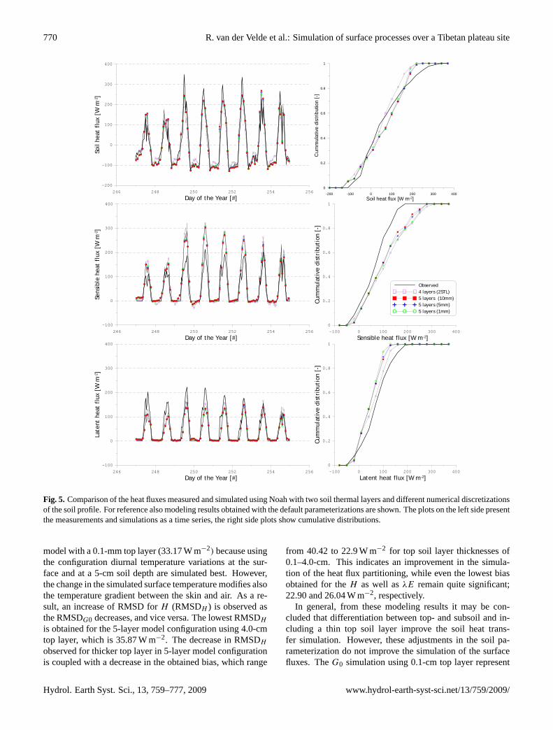
34

Fig. 5: Comparison of the heat fluxes measured and simulated using Noah with two soil

thermal layers and different numerical discretizations of the soil profile. For reference also

modeling results obtained with the default parameterizations are shown. The plots on the left

side present the measurements and simulations as a time series, the right side plots show

cumulative distributions.

246 248 250 252 254 256

Day of the Year [#]

-200

-100

0

100

200

300

400

Soil

heat

flu

x [W

m-2]

246 248 250 252 254 256

Day of the Year [#]

-100

0

100

200

300

400

Sens

ible

hea

t fl

ux [

W m

-2]

246 248 250 252 254 256

Day of the Year [#]

-100

0

100

200

300

400

Late

nt h

eat

flux

[W

m-2]

-200 -100 0 100 200 300 400Soil heat flux [W m-2]

0

0.2

0.4

0.6

0.8

1

Cum

mul

ativ

e di

strib

utio

n [-]

-100 0 100 200 300 400

Sensible heat flux [W m-2]

0

0.2

0.4

0.6

0.8

1

Cum

mul

ativ

e di

stri

buti

on [

-]

-100 0 100 200 300 400

Latent heat flux [W m-2]

0

0.2

0.4

0.6

0.8

1

Cum

mul

ativ

e di

stri

buti

on [

-]

Observed4 layers (2STL)5 layers (10mm)5 layers (5mm)5 layers (1mm)

Fig. 5. Comparison of the heat fluxes measured and simulated using Noah with two soil thermal layers and different numerical discretizationsof the soil profile. For reference also modeling results obtained with the default parameterizations are shown. The plots on the left side presentthe measurements and simulations as a time series, the right side plots show cumulative distributions.

model with a 0.1-mm top layer (33.17 W m−2) because usingthe configuration diurnal temperature variations at the sur-face and at a 5-cm soil depth are simulated best. However,the change in the simulated surface temperature modifies alsothe temperature gradient between the skin and air. As a re-sult, an increase of RMSD forH (RMSDH ) is observed asthe RMSDG0 decreases, and vice versa. The lowest RMSDH

is obtained for the 5-layer model configuration using 4.0-cmtop layer, which is 35.87 W m−2. The decrease in RMSDHobserved for thicker top layer in 5-layer model configurationis coupled with a decrease in the obtained bias, which range

from 40.42 to 22.9 W m−2 for top soil layer thicknesses of0.1–4.0-cm. This indicates an improvement in the simula-tion of the heat flux partitioning, while even the lowest biasobtained for theH as well asλE remain quite significant;22.90 and 26.04 W m−2, respectively.

In general, from these modeling results it may be con-cluded that differentiation between top- and subsoil and in-cluding a thin top soil layer improve the soil heat trans-fer simulation. However, these adjustments in the soil pa-rameterization do not improve the simulation of the surfacefluxes. TheG0 simulation using 0.1-cm top layer represent



35

Fig. 6: Same as Fig. 5, except that the measured and simulated soil temperatures are shown

for the surface and soil depth of 5-cm and 25-cm.

246 248 250 252 254 256

Day of the Year [#]

-10

0

10

20

30

40

Skin

tem

pera

ture

[o C

]

246 248 250 252 254 256

Day of the Year [#]

0

4

8

12

16

20

25-c

m S

oil t

empe

ratu

re [

o C]

246 248 250 252 254 256

Day of the Year [#]

0

5

10

15

20

25

30

5-cm

Soi

l tem

pera

ture

[o C

]

-10 0 10 20 30 40

Skin temperature [oC]

0

0.2

0.4

0.6

0.8

1

Cum

mul

ativ

e di

stri

buti

on [

-]

0 10 20 30


0

0.2

0.4

0.6

0.8

1

Cum

mul

ativ

e di

stri

buti

on [

-]

0 4 8 12 16 20


0

0.2

0.4

0.6

0.8

1

Cum

mul

ativ

e di

stri

buti

on [

-]

Fig. 6. Same as Fig. 5, except that the measured and simulated soil temperatures are shown for the surface and soil depth of 5-cm and 25-cm.

the measurements best, while differences between the mea-sured and simulatedH are smallest using a 4.0-cm top soillayer. The overestimation of theH with 0.1-cm top soil layermight suggest that the simulated solar radiation available forheating of the air and soil is too large; meaning that the sim-ulated solar radiation consumed by the cooling of surfacethrough evaporation and transpiration is too low. Further, itshould be noted that the optimized values for the quartz con-tent for the all 5-layer model configurations exceed its physi-cal limits varying between 1.50 and 1.68. An explanation forthese unrealistic values will be provided in the discussion.

5.2 Vegetation parameterization

Amelioration of inconsistencies in simulating the partition-ing betweenH and λE can be obtained by adopting anaerodynamic approach through reconsideration ofkB−1 pa-rameterization (e.g. Yang et al., 2008). However, Kahan etal. (2006) demonstrated that the simulation of the heat fluxpartitioning can also be improved by calibrating the vege-tation parameters and showed that most notably an adjust-ment in stomatal resistance is needed to increase model per-formance. Similarly, theRc,min of the Noah vegetation pa-rameterization is used, here, to improve the simulated heatflux partitioning. In addition, the optimum temperature for



Table 8. RMSD’s calculated between the measured soil temperature states and surface fluxes, and modelling results obtained with Noahconfigured to accommodate different STP for the top- and subsoil and different numerical discretizations of the soil profile.

Soil discretization H λE G0 Tskin T5cm T25cm# layers Top soil thickness [W m−2] [W m−2] [W m−2] [◦C] [◦C] [◦C]

4 layers 10.0 [cm] 52.72 33.17 41.28 1.40 1.49 1.325

laye

rs

0.1 [cm] 46.92 37.04 33.17 1.15 1.02 0.710.5 [cm] 44.34 36.21 34.73 1.25 1.05 0.681.0 [cm] 43.30 36.13 36.83 1.32 1.07 0.662.0 [cm] 43.24 36.06 39.34 1.36 1.09 0.663.0 [cm] 43.51 35.97 40.47 1.35 1.11 0.674.0 [cm] 35.87 35.89 40.68 1.35 1.03 0.67

Table 9. Same as Table 8, except the biases are presented.

Soil discretization H λE G0 Tskin T5cm T25cm# layers Top soil thickness [W m−2] [W m−2] [W m−2] [◦C] [◦C] [◦C]

4 layers 10.0 [cm] −46.40 18.70 17.33 0.84 0.30 0.44

5la

yers

0.1 [cm] −40.42 31.07 2.31 0.05 −0.21 0.670.5 [cm] −37.69 29.12 3.92 0.06 −0.28 0.651.0 [cm] −35.91 28.19 5.35 0.06 −0.30 0.632.0 [cm] −34.86 27.08 5.64 0.08 −0.29 0.643.0 [cm] −34.62 26.45 5.33 0.10 −0.28 0.644.0 [cm] −22.90 26.04 5.30 0.11 −0.25 0.65

transpiration (Topt), currently fixed at a value of 24.85◦C,may need to be tuned to represent the Tibetan conditions.

Ideally, theRc,min andTopt would be obtained from longterm data sets as has been done by Gimanov et al. (2008).This reaches, however, beyond our objective to identify theadjustments in soil and vegetation parameterization neededto improve Noah’s performance over the selected Tibetan sitefor a short 7-day period. Therefore, the parametersRc,minandTopt are calibrated by minimizing the cost function be-tween the measured and simulatedλE. For this optimizationprocedure, the 5-layer Noah model configuration is used witha 0.5 cm top soil layer and aqtzvalue of 1.58. The calibrationof theRc,min andTopt yields values of 49.88 s m−1 and 7.21◦C, respectively. Through the optimization, theRc,min is re-duced by 100.12 s m−1 andTopt by 17.61◦C in comparison tothe default parameterization. Both changes to the two plantphysiological parameters can be argued. Growing seasonson the plateau are short and, in this short period, vegetationshould be productive in order to be able to survive the harshTibetan environment. Further, temperatures on the plateauare, generally, lower than at sea level; a lower temperature atwhich plants transpire optimally is, therefore, required. Atthe same time, the validity of the defaultTopt can be ques-tioned for all environments that substantially differ from thehumid climate for the original parameterization (Dickinson,1984). A climate dependent parameterization could be con-sidered for global Noah applications, but this extends beyondthe scope of this investigation.

The modeling results of Noah simulations with the op-timized vegetation parameters are plotted against measure-ments, which are presented in Figs. 7 and 8 for the heatfluxes and soil temperatures, respectively. For comparisonpurposes, a selection of Noah simulations discussed previ-ously are also presented in Figs. 7 and 8, which are; (1) thedefault 4-layer model with the “glacial” vegetation param-eters; (2) the 4-layer model with two STL’s and “glacial”vegetation parameters; and (3) the 5-layer model with twoSTL’s, 0.5-cm top layer and “glacial” vegetation parameters.In addition, the basic statistics are presented in the plots, suchthe coefficient of determination (R2), RMSD and bias.

Comparison of the plots in Figs. 7 and 8 shows that theadjustments in the parameterization of STP improves thesimulation of the soil temperature states, but does not re-sult in a reduction in the differences between the simulatedand measured surface fluxes. Through the calibration ofthe Rc,min and Topt, the simulated partitioning betweenHandλE represents better the energy budget measurements.The RMSD’s obtained for theH andλE are reduced from47.4 and 33.2 W m−2 for the default simulations to 33.3 and26.5 W m−2 for optimized simulations, respectively. Similarresults have been presented in the Kahan et al. (2006). Theyshowed for an application of the SSiB LSM to a Sahelianstudy area that lowering the model constraints for the tran-spiration, not only increases simulatedλE, but also reducesthe overestimation in theH .



36

Fig. 7: Scatter plots of surface fluxes ( G0 , H

, λE) measured and sim

ulated using Noah in its 1)

default configuration; 2) default numerical discretizations of the soil profile and 2 STL’s; 3)

5-layer model setup, 2 STL’s and top layer of 0.5 cm

; 4) same as 3) except the vegetation

parameters are calibrated.

.

1:1 l

ine

-200 -100 0 100 200 300 400Measured G0 [W m-2]

-200

-100

0

100

200

300

400Si

mul

ated

G0

[W m

-2]

-200 -100 0 100 200 300 400Measured G0 [W m-2]

-200

-100

0

100

200

300

400

Sim

ulat

ed G

0 [W

m-2]

-200 -100 0 100 200 300 400Measured G0 [W m-2]

-200

-100

0

100

200

300

400

Sim

ulat

ed G

0 [W

m-2]

-200 -100 0 100 200 300 400Measured G0 [W m-2]

-200

-100

0

100

200

300

400

Sim

ulat

ed G

0 [W

m-2]

-100 0 100 200 300 400Measured H [W m-2]

-100

0

100

200

300

400

Sim

ulat

ed H

[W

m-2]

-100 0 100 200 300 400Measured H [W m-2]

-100

0

100

200

300

400

Sim

ulat

ed H

[W

m-2]

-100 0 100 200 300 400Measured H [W m-2]

-100

0

100

200

300

400

Sim

ulat

ed H

[W

m-2]

-100 0 100 200 300 400Measured H [W m-2]

-100

0

100

200

300

400

Sim

ulat

ed H

[W

m-2]

-100 0 100 200 300 400Measured LE [W m-2]

-100

0

100

200

300

400

Sim

ulat

ed L

E [W

m-2]

-100 0 100 200 300 400Measured LE [W m-2]

-100

0

100

200

300

400

Sim

ulat

ed L

E [W

m-2]

-100 0 100 200 300 400Measured LE [W m-2]

-100

0

100

200

300

400

Sim

ulat

ed L

E [W

m-2]

-100 0 100 200 300 400Measured LE [W m-2]

-100

0

100

200

300

400

Sim

ulat

ed L

E [W

m-2]

Soil

heat

flu

x Se

nsib

le h

eat

flux

La

tent

hea

t fl

ux4 layers (1 STL) 4 layers (2 STL) 5 layers (5mm) 5 layers (opt. veg.

params)

BIAS = 46.4 [W m-2]

R2=0.82 R2=0.85R2=0.85

BIAS = -37.6 [W m-2] BIAS = 20.8 [W m-2]BIAS = -41.3 [W m-2]

R2=0.85

RMSD = 47.4 [W m-2] RMSD = 52.7 [W m-2] RMSD = 44.34 [W m-2] RMSD = 33.3[W m-2]

BIAS = 18.7 [W m-2]

R2=0.69 R2=0.74R2=0.67

BIAS = 29.1 [W m-2] BIAS = 20.8 [W m-2]BIAS = 20.9 [W m-2]

R2=0.67


BIAS = 17.3 [W m-2]

R2=0.69 R2=0.74R2=0.67

BIAS = 3.9 [W m-2]BIAS = 2.8[W m-2]

R2=0.67


BIAS = -0.3 [W m-2]

Fig. 7. Scatter plots of surface fluxes (G0,H , λE) measured and simulated using Noah in its (1) default configuration; (2) default numericaldiscretizations of the soil profile and 2 STL’s; (3) 5-layer model setup, 2 STL’s and top layer of 0.5 cm; (4) same as (3) except the vegetationparameters are calibrated.

6 Discussion

The adjustments in the parameterization of the STP and cal-ibration of the vegetation parameters,Rc,min andTopt, haveameliorated the simulation of the soil heat transfer and re-duced uncertainties in the simulatedH and λE to levelscomparable as are reported in previous investigations (e.g.,Sridhar et al., 2003; Gutmann and Small, 2007; and Pauwelset al., 2008). Despite the optimized Noah simulations areable to represent the soil temperature and surface energy bal-ance measurements better, still some inconsistencies in themodeling results can be observed when radiative forcingsbecome large. For example, Noah systematically overesti-mates the measuredH at values larger than approximately150 W m−2, which coincides with underestimation of theG0andTskin when the measured values are larger than approx-imately 150 W m−2 and 20◦C, respectively. Apparently, un-der large radiative forcings Noah is not able to simulateTskinincrease measured on the Tibetan Plateau. Therefore, thesimulated temperature gradients between the surface and at-mosphere, and between surface and the mid-point of the first

soil layer become too large and too small, respectively. As aresult, an over- and underestimation of the measuredH andG0 are observed. The explanation of this discrepancy in thesimulatedTskin is twofold.

First, the surface exchange coefficient for heat (Ch) maynot be properly parameterized for the Tibetan conditions.Noah uses the Reynolds number dependent method pro-posed by Zilintinkevich (1995) to determine thekB−1. How-ever, Yang et al. (2008) showed for bare soil surfaces thatReynolds number dependentkB−1 methods, in general, tendto underestimate the strong diurnalkB−1 variations observedover the Tibetan Plateau (e.g. Ma et al. 2005 and Yang etal. 2003). AkB−1underestimation during daytime resultsin more efficient heat transfer between the soil surface andthe atmosphere, which causes anH overestimation and ex-plains also the discrepancy between the measured and sim-ulatedTskin. OtherkB−1 methods (e.g. Su et al. 2001 andYang et al. 2002) that are able to capture this diurnalkB−1

variation would further improve Noah’s overall performanceover the Tibetan Plateau. This reaches, however, beyond thescope of this investigation. For evaluations of the available


774 R. van der Velde et al.: Simulation of surface processes over a Tibetan plateau site 37

Fig. 8: Same as Fig. 7 expect that the tem

perature states (Tskin , T

5cm and T25cm ) are show

n here.

0 5 10 15 20Measured T25cm [oC]

0

5

10

15

20

Sim

ulat

ed T

25cm

[o C

]

1:1 l

ine

-10 0 10 20 30 40Measured Tskin [oC]

-10

0

10

20

30

40Si

mul

ated

Tsk

in [

o C]


-10

0

10

20

30

40

Sim

ulat

ed T

skin [

o C]


-10

0

10

20

30

40

Sim

ulat

ed T

skin [

o C]


-10

0

10

20

30

40

Sim

ulat

ed T

skin [

o C]

0 5 10 15 20 25 30Measured T5cm [oC]

0

5

10

15

20

25

30

Sim

ulat

ed T

5cm [

o C]

0 5 10 15 20 25 30Measured T5cm [oC]

0

5

10

15

20

25

30

Sim

ulat

ed T

5cm [

o C]

0 5 10 15 20 25 30Measured T5cm [oC]

0

5

10

15

20

25

30

Sim

ulat

ed T

5cm [

o C]

0 5 10 15 20 25 30Measured T5cm [oC]

0

5

10

15

20

25

30

Sim

ulat

ed T

5cm [

o C]


0

5

10

15

20

Sim

ulat

ed T

25cm

[o C

]


0

5

10

15

20

Sim

ulat

ed T

25cm

[o C

]


0

5

10

15

20

Sim

ulat

ed T

25cm

[o C

]

Skin

Tem

pera

ture

5-

cm s

oil t

empe

ratu

re

25-c

m s

oil t

empe

ratu

re4 layers (1 STL) 4 layers (2 STL) 5 layers (5mm) 5 layers (opt. veg.

params)

BIAS = 0.30 [oC]

R2=0.98 R2=0.95R2=0.92

BIAS = -0.28 [oC] BIAS = 1.17 [oC]BIAS = 0.10 [oC]

R2=0.88

RMSD = 1.28 [oC] RMSD = 1.49 [oC] RMSD = 1.05 [oC] RMSD = 1.17 [oC]

BIAS = 0.44 [oC]

R2=0.95 R2=0.90R2=0.55

BIAS = 0.65 [oC] BIAS = 1.09 [oC]BIAS = 0.45 [oC]

R2=0.51

RMSD = 1.33 [oC] RMSD = 1.32 [oC] RMSD = 0.68 [oC] RMSD =1.10 [oC]

BIAS = 0.84 [oC]

R2=0.99 R2=0.99R2=0.98

BIAS = 0.06 [oC]BIAS = 0.56 [oC]

R2=0.98

RMSD = 1.45 [oC] RMSD = 1.40 [oC] RMSD = 1.25 [oC] RMSD = 1.43 [oC]

BIAS = 1.49 [oC]

Fig. 8. Same as Fig. 7 expect that the temperature states (Tskin, T5cm andT25cm) are shown here.

kB−1 methods readers are referred to Liu et al. (2007) andYang et al. (2008).

Second, the linearization of the surface energy balance(see Eq. (10)) utilized to compute theTskin contributes toexplaining the differences between the simulated and mea-suredTskin. This approximation is exact whenTair is equiv-alent toTskin and loses its validity as the difference betweenTair andTskin increases. For our Tibetan study site, differ-ences between theTair andTskin can be expected to be sig-nificantly larger than at sea level because the air pressure ismuch lower and fewer air molecules are available to transportenergy from the surface towards the air. To demonstrate theimpact of the applied approximation for our Tibetan site, themeasuredTskin andTair, theTskin calculated by using Eq. (10)and are plotted in Fig. 9. This plot shows that the applied ap-proximation holds rather well during nighttime. After sun-rise, however, differences between measuredTair andTskinincrease resulting in a discrepancy between the measured andapproximatedTskin of more than 10◦C at midday. Obviously,this leads to an underestimation ofTskin even when the pa-rameterization of the soil-vegetation-atmosphere system isagreement with the local conditions.

Within the uncertainties embedded in theCh calculationand in the linearization applied for theTskin simulation liesalso the explanation for the unrealistically high values of thecalibrated qtz parameter. With the increase of the qtz param-eter, the thermal heat conductance is raised to increase thetransport of heat into soil and to compensate for the lowersimulated temperature gradient between surface and the midpoint of the first soil layer. When the qtz parameter is notused to compensate for theTskin underestimation, biases arisein the simulation of the soil temperature profile as occurs inNoah applications in the default configuration.

Another issue in the default Noah configuration that hasnot been addressed in the text above is the LAI value, whichis fixed at a value of 5.0 m2 m−2. To evaluate the influenceof this LAI value on the results presented in this study, theoptimization of the qtz parameter has been performed usinga LAI of 1.2 m2 m−2 (obtained from the MODIS LAI prod-uct) for the Noah 4- and 5-layer configurations with 2 STL’s,whereby for the 5-layer configuration a top soil thickness of0.5 cm was used. This optimization results in qtz values 0.66and 1.45 for the 4- and 5-layer discretization, respectively.The optimized qtz parameters are lower and, thus, in the case



38

Fig. 9: Measurements of the air and surface temperature, and the surface temperature

approximated using Eq. 10 plotted as a time series for the analyzed period of meteorological

forcing collected at a Tibetan Plateau site.

246 248 250 252 254 256

Day of the Year [#]

-10

0

10

20

30

40

Tem

pera

ture

[o C

]

Air temperatureMeasured TskApproximated Tsk

Fig. 9. Measurements of the air and surface temperature, and the surface temperature approximated using Eq. (10) plotted as a time seriesfor the analyzed period of meteorological forcing collected at a Tibetan Plateau site.

of the 5-layer configuration closer to a value that is realisti-cally possible, but is still far too high.

Using the qtz value of 1.45 and 5-layer discretization witha 0.5 cm top layer, the vegetation parameters,Rc,min andTopt,have also been recalibrated with a LAI of 1.2 m2 m−2, whichresults in values of 20.89 s m−1 and 9.73◦C, respectively.Compared to the vegetation parameter presented above, theRc,min has decreased by more than a factor two, while theTopt has increased only slightly. This large reduction inRc,min follows directly from Eq. (24), in which theRc,minand LAI have an opposite effect on the calculation of theRc.Thus, the decrease in LAI is for a large part compensatedwithin the model calibration by decreasing theRc,min.

As to determine whether using the MODIS LAI improvesNoah’s performance, RMSD values between the measuredand simulated soil temperatures and heat fluxes have beencomputed for the three additional Noah simulations and arepresented in Table 10. Comparison of the RMSD values ofTable 10 with the results presented previously shows thatthe simulation of the temperatures across the soil profile im-proves somewhat. However, Noah’s overall ability to simu-late the heat fluxes decreases when using the MODIS LAI.Apparently, Noah has been tuned to perform optimally usingLAI of 5.0 m2 m−2, which is probably the reason for using afixed value for large-scale Noah applications.

7 Conclusions

In this paper, adjustments in the soil and vegetation param-eterizations required to be able to reproduce the soil tem-perature states and surface fluxes using the Noah LSM areinvestigated using a 7-day period of in-situ measurementscollected at a study site on the Tibetan Plateau. Analysis

Table 10. RMSD values calculated between soil temperatures andsurface fluxes measured and simulated by Noah using a LAI valueof 1.2 m2m−2; 4-layer∼ Noah simulations obtained with the de-fault 4 layer soil discretization and calibrating theqtz parameter(=0.66); 5-layer∼ Noah simulation obtained using 5 layers (toplayer=0.5 cm) and calibrating the qtz parameter (=1.45); 5l+veg∼

Noah simulations obtained 5-layer soil discretization and qtz pa-rameter and calibrating the vegetation parametersRc,min andTopt

(20.89 s m−1 and 9.73◦C).

H λE G0 Tskin T5cm T25cm[W m−2] [W m−2] [W m−2] [◦C] [◦C] [◦C]

4 layer 67.29 43.46 38.64 1.48 1.08 1.195 layer 58.74 50.92 35.81 0.97 1.04 0.515l+veg. 35.41 26.85 33.78 1.33 1.18 1.09

of the results from simulations obtained through applicationof the default parameterization has shown that (1) heat trans-fer through the soil column is not represented adequately, (2)partitioning between the sensible (H ) and latent heat (λE)flux is biased. Amelioration of the parameterization of theseland surface processes is achieved through adjustment of soiland vegetation parameterizations.

Through differentiating between the soil thermal proper-ties of a top- and subsoil, and including a thin top soil layer,uncertainties in the simulation of the soil heat transfer arereduced and RMSD’s between the measured and simulatedTskin, T5cm and T25cm are obtained of 1.25◦C, 1.05◦C and0.68◦C by using a 0.5 cm thick top soil layer. It is found thatadding a thin top soil layer has stronger effect than differ-entiating between the soil thermal properties of a top- andsubsoil. A decrease in the vegetation parameters,Rc,min andTopt, constraining the transpiration reduces the RMSD for the



λE from 33.2 W m−2 obtained using the default Noah con-figuration to 26.5 W m−2 using the optimized parameteriza-tion. In addition, the improvement in theλE simulation alsoinfluences theH simulation and decreases the RMSD from47.41 to 33.3 W m−2, while the differences between the mea-sured and simulatedG0 do not change significantly.

Although the adjustments in the parameterization of theSTP and calibration of vegetation parameters improvedNoah’s capability of representing the soil temperature statesand the surface energy balance components measured onthe Tibetan Plateau, under conditions of the high radiativeforcings an underestimation is observed of measuredTskin.This underestimation of theTskin results in an overestimationof theH and underestimationG0. The explanation for thediscrepancy in theTskin simulation is twofold. First, thesurface exchange coefficient for heat may not be properlyparameterized. Second, the approximation, adopted forlinearization of the surface energy balance for theTskincalculation, introduces some uncertainties when differencesbetween the measuredTskin and Tair are large, which aretypical midday conditions on the Tibetan Plateau.

Edited by: J. Wen

References

Chen, F., Janjic, Z., and Mitchell, K.: Impact of atmosphericsurface-layer parameterizations in the new land-surface schemeof the NCEP mesoscale ETA model, Bound.-Lay. Meteorol., 85,391–421, 1997.

Cosby, B. J., Hornberger, G. M., Clapp, R. B., and Ginn, T. R.:Water Resour. Res., 20, 682-690, 1984.

Dickinson, R. E.: Modeling evapotranspiration for three-dimensional global climate models, in: Climate processes andclimate sensitivity, editedy by: Hansen, J. E. and Takahashi, T.,American Geophysical Union, Geophys. Monogr., 29, 58–72,1984.

Dickinson, R. E., Oleson, K. W., Bonan, G., Hoffman, F., Thornton,P., Vertenstein, M., Yang, Z.-L., and Zeng, X.: The communityland model and its climate statistics as a component of the com-munity climate system model, J. Climate, 19, 2302–2324, 2006.

Doherty, J.: Manual for the PEST Surface Water Modelling Util-ities, Watermark Numerical Computing, Australia, available athttp://www.sspa.com/pest, 2003.

Duan, Q., Schaake, J., Andreassian, V., et al.: Model parameter es-timation experiment (MOPEX): An overview of science strategyand major results from the second and third workshops, J. Hy-drol., 320, 3–17, 2006.

Ek, M. B., Mitchell, K. E., Lin, Y., Rogers, E., Grunmann, P., Ko-ren, V., Gayno, G., and Tarpley, J. D.: Implementation of Noahland surface model advances in the National Centers for Environ-mental Prediction operational mesoscale Eta model, J. Geophys.Res., 108, 8851, doi:10.1029/2002JD003296, 2003.

Gallagher, M. and Doherty, J.: Parameter estimation and uncer-tainty analysis for a watershed model, Environ. Modell. Softw.,22, 1000–1020, 2007.

Garratt, J. R.: Sensitivity of climate simulations to land-surface andatmospheric boundary-layer treatments – A review, J. Climate, 6,419-448, 1993.

Gilmanov, T. G., Soussana, J. F., Aires, L., et al.: Partitioning Euro-pean grassland net ecosystem CO2 exchange into gross primaryproductivity and ecosystem respiration using light response func-tion analysis, Agr. Ecosyst. Environ., 121, 93–120, 2007.

Gutmann, E. D. and Small, E. E.: A comparison of land surfacemodel soil hydraulic properties estimated by inverse modelingand pedotransfer functions, Water Resour. Res., 43, W05418,doi:10.1029/2006WR005135, 2007.

Gulden, L. E., Rosero, E., Yang, Z., Rodell, M., Jackson, C.S., Niu, G., Yeh, P. J.-F., and Famiglietti, J.: Improving land-surface model hydrology: Is an explicit aquifer model betterthan a deeper soil profile?, Geophys. Res. Lett., 34, L09402,doi:10.1029/2007GL029804, 2007.

Hillel, D.: Environmental soil physics, Academic Press, 771 pp.,1998.

Hogue, T. S., Bastidas, L., Gupta, H., Sorooshian, S., Mitchell, K.,and Emmerich, W.: Evaluation and transferability of the Noahland surface model in semiarid environments, J. Hydrometeorol.,6, 68–83, 2005.

International GEWEX Project Office: GSWP-2: The SecondGlobal Soil Wetness Project Science and Implementation Plan.IGPO Publication Series No. 37, 65 pp., 2002.

Jacquemin, B. and Noilhan, J.: Sensitivity study and validation ofa land surface parameterization using the HAPEX-MOBILHYdata set, Bound.-Lay. Meteorol., 52, 93–134, 1990.

Jarvis, P. G.: The interpretation of the variations in leaf water po-tential and stomatal conductance found in canopies in the field,Philos. T. Roy. Soc. B, 273, 593–610, 1976.

Johansen, O.: Thermal conductivity of soils. Ph.D thesis, Universityof Trondheim, 236 pp., 1975.

Kahan, D. S., Xue, Y., and Allen S. J.: The impact of vegetationand soil parameters in simulations of surface energy and waterbalance in the semi-arid sahel: A case study using SEBX andHAPEX-Sahel data, J. Hydrol., 320, 238–259, 2006.

Kato, H., Rodell, M., Beyrich, F., Cleugh, H., van Gorsel, E., Liu,H., and Meyers, T. P.: Sensitivity of land surface simulations tomodel physics, land characteristics, and forcings, at four CEOPSites, J. Meteorol. Soc. Jpn., 87A, 187–204, 2007.

Kersten, M. S.: Thermal properties of soils. University of Min-nesota Engineering Experiment Station Bulletin 28, 227 pp.,available from University of Minnesota Agricultural ExperimentStation, St. Paul, MN 55108, 1949.

Koster, R. D., Dirmeyer, P. A., Guo, Z., et al.: Regions of strongcoupling between soil moisture and precipitation, Science, 305,1138–1140, 2004.

Liu, S., Lu, L., Mao, D., and Jia, L.: Evaluating parameterizationsof aerodynamic resistance to heat transfer using field measure-ments, Hydrol. Earth Syst. Sci., 11, 769–783, 2007,http://www.hydrol-earth-syst-sci.net/11/769/2007/.

Ma, Y., Tsukamoto, O., Wang, J., Ishikawa, H., and Tamagawa, I.:Analysis of aerodynamic and thermodynamic parameters on thegrassy marshland surface of Tibetan Plateau, Prog. Nat. Sci., 12,36–40, 2002.


http://www.sspa.com/pest

http://www.hydrol-earth-syst-sci.net/11/769/2007/


Ma, Y., Fan, S., Ishikawa, H., Tsukamoto, O., Yao, T., Koike, T.,Zuo, H., Hu, H., and Su, Z.: Diurnal and inter-monthly variationof land surface heat fluxes over the central Tibetan Plateau area,Theor. Appl. Climatol., 80, 259–273, 2005.

Ma, Y., Menenti, M., Feddes, R., and Wang, J.: Analysis of the landsurface heterogeneity and its impact on atmospheric variablesand the aerodynamic and thermodynamic roughness lengths, J.Geophys. Res., 113, D08113, doi:10.1029/2007JD009124, 2008.

Mahfouf, J. F. and Noilhan, J.: Comparative study of various for-mulation of evaporation from bare soil using in situ data, J. Appl.Meteorol., 30, 1354–1365, 1991.

Marht, L. and Ek, M.: The influence of atmospheric stability on po-tential evaporation, J. Clim. Appl. Meteorol., 23, 222–234, 1984.

Marht, L. and Pan, H.-L.: A two-layer model of soil hydrology,Bound.-Lay. Meteorol., 29, 1-20, 1984.

McCumber, M. C. and Pielke, R. A.: Simulation of the effects ofsurface fluxes of heat and moisture in a mesoscale numericalmodel 1. soil layer, J. Geophys. Res., 86, 9929–9938, 1981.

Mitchell, K., Lohmann, D., Houser, P. R., et al.: The multi-institution North American Land Data Assimilation System (NL-DAS): Utilizing multiple GCIP products and partners in a con-tinental distributed hydrological modeling system, J. Geophys.Res., 109, D07S90, doi:10.1029/2003JD003823, 2004.

Pan, H.-L., and Marht, L.: Interaction between soil hydrology andboundary-layer development, Bound.-Lay. Meteorol., 38, 185–202, 1987.

Pauwels, V. R. N. and Samson, R.: Comparison of different meth-ods to measure and model actual evapotranspiration rate for a wetsloping grassland, Agr. Water Manage., 82, 1–24, 2006.

Pauwels, V. R. N., Timmermans, W., and Loew, A. Comparison ofthe estimated water and energy budgets of a large winter wheatfield during AgriSAR 2006 by multiple sensors and models, J.Hydrol., 349, 425–440, 2008.

Perez, P. J., Castellvi, F., Ibanez, M., and Rosell, J. I.: Assessmentof reliability of Bowen ratio method for partitioning fluxes, Agr.Forest Meteorol., 97, 141–150, 1999.

Peters-Lidard, C. D., Blackburn, E., Liang, X., and Wood, E. F.:The effect of soil thermal conductivity parameterization on sur-face energy fluxes and temperatures, J. Atmos. Sci., 55, 1209–1224, 1998.

Rodell, M., Houser, P. R., Jambor, U., Gottschalck, J., Mitchell,K., Meng, C.-J., Arsenault, K., Cosgrove, B., Radakovich, J.,Bosilovich, M., Entin, J. K., Walker, J. P., Lohmann, D., andToll, D.: The Global Land Data Assimilation System, B. Am.Meteorol. Soc., 85(3), 381–394, 2004.

Schaake, J. C., Koren, V. I., Duan, Q.-Y., Mitchell, K., and Chen,F.: Simple water balance model for estimating runoff at differentspatial and temporal scales, J. Geophys. Res., 101, 7461–7575,1996.

Schaake, J., Duan, Q., Andreassian, V., Franks, S., Hall, A.,and Leavesley, G.: The model parameter estimation experimentMOPEX, J. Hydrol., 349, 425–440, 2006.

Su, Z., Schmugge, T., Kustas, W. P., and Massman, W. J.: An eval-uation of two models for estimation of the roughness length forheat transfer between the land surface and the atmosphere, J.Appl. Meteorol., 40, 1933–1951, 2001.

Sridhar, V., Elliott, R.L., Chen, F., and Brotzge, J. A.: Valida-tion of the Noah-OSU land surface model using surface fluxmeasurements in Oklahoma, J. Geophys. Res., 107(D20), 4418,doi:10.1029/2001JD001306, 2002.

de Vries, D. A.: Thermal properties of soils. Physics of Plant Envi-ronments, edited by: van Wijk, W. R., Noord-Holland, 210-235,1963.

Xue, Y., Sellers, P. J., Kinter, J. L., and Shukla, J.: A simplifiedbiosphere model for global climate studies, J. Climate, 4, 345–364, 1991.

Yang, K., Koike, T., Fujii, H., Tamagawa, K., and Hirose, N.: Im-provement of surface flux parameterizations with a turbulence-related length, Q. J. Roy. Meteor. Soc., 128, 2073–2087, 2002.

Yang, K., Koike, T., and Yang, D.: Surface flux parameterization inthe Tibetan Plateau, Bound.-Lay. Meteorol., 116, 245-262, 2003.

Yang, K., Koike, T., Ye, B., and Bastidas, L.: Inverse analysisof the role of soil vertical heterogeneity in controlling surfacesoil state and energy partition, J. Geophys. Res., 110, D08101,doi:10.1029/2004/JD005500, 2005.

Yang, K., Koike, T., Ishikawa, H., Kim, J., Li, X., Liu, H., Liu, S.,Ma, Y., and Wang, J.: Turbulent flux transfer over bare-soil sur-faces: Characteristics and Parameterizations, J. Appl. Meteorol.Clim., 47, 276–290, 2008.

Zeng, X. and Dickinson, R. E.: Effect of surface sublayer on surfaceskin temperature and flux, J. Climate, 11, 537–550, 1998.

Zilitinkevich, S. S.: Non-local turbulent transport: Pollution dis-persion aspects of coherent structure of convective flow, in: AirPollution, Vol. 1, Air Pollution Theory and Simulation, editedby: Power, H., Moussiopoulos, N., and Brebbia, C. A., Compu-tational Mechanics Publication, Southampton, 53–60, 1995.


Documents

Inﬂuence of thermodynamic soil and vegetation ... · PDF fileInﬂuence of thermodynamic soil and vegetation parameterizations on the simulation of soil temperature states ... Experiment