Embed Size (px)
Citation preview

Influence of baryonic matter on the galactic halostructure and its satellites
Diplomarbeit an der Fakultät für Physikder Universität Bielefeld
Mai 2010
JASCHA SCHEWTSCHENKO
Betreuer / Prüfer
Prof. Dr. Dominik SchwarzUniversität Bielefeld
Fakultät für PhysikUniversitätsstraße 25
33615 Bielefeld
Dr. Andrea MacciòMax-Planck-Institut für AstronomieGalaxy Theory GroupKönigsstuhl 1769117 Heidelberg


ABSTRACT
In this thesis, we examine the effects of baryonic matter on galaxy halos and in-falling satellites, i.e accreted substructures in these halos. We hereby focus on theirmass evolution as well as some specific parameters of their orbits. The analysisis based on data of several pairs of numerical simulations each consisting of a pureDM and a hydrodynamical simulation run with (nearly) identical initial conditions.We identify then pairs of satellites that share the same origin in the initial condi-tions and therefore a similar formation history. Motivated by a result obtained byMacciò et al. [MMSD06], that shows a discrepancy in the number density profilesof the substructures for the two different simulation types, we confirmed this in-creased number of satellite in the inner region of the main halo in the hydrodynam-ical simulations and explained it by a increased dynamical fraction in the denserinner region of the ”hydro” main halos as they contain cool gas and stars insteadof just dark matter, which steepens the density profile significantly. We hereby de-termined this difference in the density and potential profiles of the main halo us-ing several popular models (NFW, GNFW & PoLLS). These results are furthermoreused to extrapolate the pericentric, apocentric and average distance for each satel-lite and corresponding partner, which is used to further analyze the origin of thedifference in radial distribution. Additionally we analyze the mass loss in each sim-ulation type for each pair of satellites and find, that, despite an expected higher sta-bility of hydrodynamical structures, the innermost satellites are losing much moremass than their DM counterpart. This more intensive stripping could be explainedby the decreased average distance that favors the tidal stripping. This result is inso far surprising as it implicates a shorter life expectancy of the inner satellites inthe hydrodynamical simulation, which works against the observered difference innumber density profile instead of supporting it. Finally, we use our results to brieflydiscuss whether they increase or decrease the danger for the galactic disk by closeencounters with heavy satellites.
i


There is a theory which states that if ever for any reason anyone discovers whatexactly the Universe is for and why it is here it will instantly disappear and be
replaced by something even more bizarre and inexplicable. There is another thatstates that this has already happened.
— Douglas Adams
ACKNOWLEDGMENTS
I would like to thank all those who made this thesis possible. I am heartily thankfulto my supervisor, Dr. Andrea Macciò, whose guidance, support and patience fromthe beginning to the completion of this work were an invaluable help for me duringthe whole time. I also thank my supervisor in Bielefeld, Prof. Dr. Dominik Schwarz,who sparked my interest for cosmology by his lectures and seminars in the firstplace and provided important advice for this thesis during my visits in Bielefeld.
I further owe my deepest gratitude to my parents, who supported me not only fi-nancially, but also, much more importantly, emotionally by providing a confidencein my work and my whole academical career so far, especially at times when I lostit myself.
And, lastly, I offer my regards to all of those not mentioned before who supportedme in any respect during the completion of this work. This includes especially myflat mates and my office mates who had to ”endure” me for the whole year andhelped me to stay at least slightly in touch with the world beside the work for thisthesis.
Bielefeld, Mai 2010
iii


CONTENTS
Abstract i
Acknowledgements iii
I Preamble ix
Motivation xi
Overview xii
II Background / Preparatory work xv
1 Cosmology 11.1 History of Cosmology . . . . . . . . . . . . . . . . . . . . . . . . . . . 11.2 Cosmic Microwave Background / Matter Power Spectrum . . . . . . 41.3 Fundamentals of Cosmology . . . . . . . . . . . . . . . . . . . . . . . 7
1.3.1 Fundamental principles . . . . . . . . . . . . . . . . . . . . . . 71.3.2 Metric . . . . . . . . . . . . . . . . . . . . . . . . . . . . . . . . 81.3.3 Cosmological Stress-Energy-Momentum Tensor . . . . . . . . 91.3.4 Dynamics . . . . . . . . . . . . . . . . . . . . . . . . . . . . . . 91.3.5 Redshift . . . . . . . . . . . . . . . . . . . . . . . . . . . . . . . 10
1.4 Cosmological Models . . . . . . . . . . . . . . . . . . . . . . . . . . . . 111.4.1 Nature of Dark Matter . . . . . . . . . . . . . . . . . . . . . . . 121.4.2 Standard ΛCDM- Model . . . . . . . . . . . . . . . . . . . . . . 12
2 Structures in the Universe 172.1 Structure Formation & Evolution . . . . . . . . . . . . . . . . . . . . . 17
2.1.1 Newtonian cosmology & Comoving coordinates . . . . . . . . 182.1.2 Density perturbation dynamics and Zel’dovich approximation 202.1.3 Spherical Collapse Model . . . . . . . . . . . . . . . . . . . . . 232.1.4 Virialization . . . . . . . . . . . . . . . . . . . . . . . . . . . . . 242.1.5 Press-Schechter Theory & Mergers . . . . . . . . . . . . . . . . 25
v

2.1.6 Interaction: Dynamical friction & Tidal Stripping . . . . . . . 272.2 Density/Potential profiles . . . . . . . . . . . . . . . . . . . . . . . . . 29
2.2.1 Singular Isothermal Sphere Model . . . . . . . . . . . . . . . . 302.2.2 Zhao’s (α, β, γ)-Models . . . . . . . . . . . . . . . . . . . . . . 312.2.3 PoLLS / Einasto model . . . . . . . . . . . . . . . . . . . . . . 332.2.4 Comparison . . . . . . . . . . . . . . . . . . . . . . . . . . . . . 36
3 Numerical simulations 393.1 Discretization techniques . . . . . . . . . . . . . . . . . . . . . . . . . . 40
3.1.1 Space . . . . . . . . . . . . . . . . . . . . . . . . . . . . . . . . . 403.1.2 Time / Time integration . . . . . . . . . . . . . . . . . . . . . . 42
3.2 Overview: Simulation techniques . . . . . . . . . . . . . . . . . . . . . 463.2.1 CDM N-body simulations . . . . . . . . . . . . . . . . . . . . . 463.2.2 Hydrodynamical simulations . . . . . . . . . . . . . . . . . . . 53
3.3 Initial conditions . . . . . . . . . . . . . . . . . . . . . . . . . . . . . . 593.3.1 Resolution refinement / Zoom technique . . . . . . . . . . . . 593.3.2 Baryonic matter . . . . . . . . . . . . . . . . . . . . . . . . . . . 60
3.4 Actual Simulations . . . . . . . . . . . . . . . . . . . . . . . . . . . . . 603.4.1 Simulation codes . . . . . . . . . . . . . . . . . . . . . . . . . . 613.4.2 Runs & Parameters . . . . . . . . . . . . . . . . . . . . . . . . . 64
4 Evaluation tools 674.1 Main Halo . . . . . . . . . . . . . . . . . . . . . . . . . . . . . . . . . . 67
4.1.1 Finding / Tracking . . . . . . . . . . . . . . . . . . . . . . . . . 674.1.2 Density fitting . . . . . . . . . . . . . . . . . . . . . . . . . . . . 68
4.2 Satellites . . . . . . . . . . . . . . . . . . . . . . . . . . . . . . . . . . . 704.2.1 Finding / Grouping . . . . . . . . . . . . . . . . . . . . . . . . 704.2.2 Tracking . . . . . . . . . . . . . . . . . . . . . . . . . . . . . . . 744.2.3 ”Twin” Matching . . . . . . . . . . . . . . . . . . . . . . . . . . 754.2.4 Orbits . . . . . . . . . . . . . . . . . . . . . . . . . . . . . . . . 77
III Evaluation 81
5 Evaluation/Comparison of Galaxy Halos 83
6 Evaluation/Comparison of Satellites 916.1 Comparison of radial positions/orbits . . . . . . . . . . . . . . . . . . 936.2 Comparison of Mass & Mass Loss . . . . . . . . . . . . . . . . . . . . 1056.3 ”Impact on Galaxy Disk” . . . . . . . . . . . . . . . . . . . . . . . . . . 115
7 Conclusion 117
Bibliography 119
List of Figures 124
IV Appendix 129
A Implementation of Analysis Pipeline 131
vi

Contents vii
A.1 Code overview . . . . . . . . . . . . . . . . . . . . . . . . . . . . . . . 131A.1.1 Input and Internal representation . . . . . . . . . . . . . . . . 131A.1.2 Smoothing & Grouping . . . . . . . . . . . . . . . . . . . . . . 132A.1.3 Satellite tracking & Twin matching . . . . . . . . . . . . . . . . 132A.1.4 Halo finding . . . . . . . . . . . . . . . . . . . . . . . . . . . . . 133A.1.5 Density fitting . . . . . . . . . . . . . . . . . . . . . . . . . . . . 133A.1.6 Orbits . . . . . . . . . . . . . . . . . . . . . . . . . . . . . . . . 133
A.2 Tools . . . . . . . . . . . . . . . . . . . . . . . . . . . . . . . . . . . . . 134A.3 Compilation / Installation . . . . . . . . . . . . . . . . . . . . . . . . . 134A.4 Future prospects . . . . . . . . . . . . . . . . . . . . . . . . . . . . . . . 134
A.4.1 OOP . . . . . . . . . . . . . . . . . . . . . . . . . . . . . . . . . 134A.4.2 TIPSY Analysis library . . . . . . . . . . . . . . . . . . . . . . . 135
B Satellite tracking 137B.1 Cases . . . . . . . . . . . . . . . . . . . . . . . . . . . . . . . . . . . . . 137B.2 Algorithm . . . . . . . . . . . . . . . . . . . . . . . . . . . . . . . . . . 140
C Plots / Results 143C.1 Evaluation/Comparison of Galaxy Halos . . . . . . . . . . . . . . . . 143C.2 Comparison of Satellite ”twins” . . . . . . . . . . . . . . . . . . . . . . 150


Part I
Preamble


Contents xi
Motivation
In this thesis we study the difference in structure formation and satellite accred-ition of pure dark matter (DM) and hydrodynamical (Hydro) simulation. Usingcomparable simulation code (pkdGrav & Gasoline) as well as comparable initialconditions (cf. Ch. 3.4) enabled us to obtain results for both types of simulationswithout having to worry much that observed differences are code-related. Hence,this allows us to explicitly study the differences of the properties and dynamics ofsmall halos that are accreted by a larger main halo during the runs of the cosmo-logical simulation, that are only caused by applying hydrodynamics on a baryonicsubcomponent of the matter. Thereby a few publications motivated and guided ouranalysis as we will outline in the following subsections:
Radial distribution - Macciò (2006)
The initial motivation to study closer the differences of the statistics and dynamicsof satellite accredition in the DM and Hydro simulations was given by work of Mac-ciò et al. [MMSD06] wherein has been discovered that there is a significant increasein the numbers of satellites in the inner regions of the host halo as can be seen inFig.1 and 2.
FIGURE 1: Ratio of the number of DM subhaloeswith M > 2 · 108 M in the hydro and dm runs asa function of the distance from the center of themain halo [MMSD06, Fig.5]
FIGURE 2: Substructure radial density profilesfor different simulations [MMSD06, Fig.6]
The question that arise here is which influence of the baryonic matter leads to theseresults. To answer this, we study ”twins” of satellites in both simulation, i.e. struc-tures that have (nearly) the same formation history in both simulation types due tothe same initial conditions. This then allows us to clarify if the result of Maccio canbe observed by comparing the pairs of twins instead and to observe possible causesfor this effect by comparing the twins.

xii Contents
Impact on Galaxy Disk - Moster (2010) / Kazantzidis (2009)
Another motivation for further studies concerning the different results of pure darkmatter and hydrodynamical simulations arises in the context of two papers that areboth examining the dynamical effects of hierarchical satellite accretion. Moster et al.[MMS+10] did this by constructing an initial system of satellites around a centralgalaxy based on analytical models. While Kazintzidis et al. [KZK+09] used a similarapproach, they also used the results of pure DM simulations to obtain ”realistic”initial phase-space coordinates for the modelled satellites as shown in Fig.3
FIGURE 3: Scatter plot of pericentric distance versus satellite mass. Filled symbols thereby representthe satellites that cross within a radius of 50 kpc after z = 1 while unfilled symbols mark the propertiesof surviving substructures at z = 0[KZK+09, Fig.1]
While Moster has concluded that gas has a positive impact on the stability of aGalaxy disk if faced with close approaches of satellites. The question we are nowinterested in is how does the same baryonic matter influence the risk that dangerousclose encounters take place. As mentioned, Maccio already observed a higher num-ber density at z = 0 in the inner region for Hydro simulation. So, by comparing theresults for pairs of twins and tracking these through time, we can conclude whetherthe satellites in the hydrodynamical simulation impose a greater thread, based ontheir mass and pericentric distance than their matching DM counterparts.
Overview
Concluding this preamble, we want to provide a brief overview over this thesis,which has been divided into three major parts.

Contents xiii
The first one contains the Background and Preparatory needed to understand howthe results of this thesis have been obtained. The first chapter provides an introduc-tion into Cosmology, which is the broader field we are dealing with. We thereby putan emphasis on describing the basics of modern cosmology that leads to the currentstandard model, on which our simulations are based.After having introduced the overall dynamics of the Universe, Chapter 2 deals nowwith the formation and evolution of specific large-scale structures in the later uni-verse, i.e. (galaxy) halos. We first introduce linear theories of structure formationup to the Zel’dovich approximation that will become important to construct initialconditions for our simulations. Subsequently, we discuss the theories of halo col-lapse and virialization that form two major aspects of the structures of interest. Thesecond half of this chapter is then devoted to review and compare several analyti-cal models for the density profile of the halos we want to analyze. Instead of simplyrelying on the standard NFW model, we present some generalizations and the SISmodel that will be then compared by analyzing their efficiency to approximate thedensity profile of the main halo and its satellite halos that we had found in the sim-ulation data.Chapter 3 finally reviews several numerical methods. This includes the techniquesof the simulation code, that we used to get our data, as well as e.g. time integrationschemes that we used to develop the tools for our analysis.These tools are then the subject of the discussion in Chapter 4 which concludes theBackground part. We explain there which methods we had to use and to develop tostudy the structure and the dynamics of both the main halo and its satellites, that itis going to accrete or already has accreted.
The second part now deals with the analysis itself. It starts with chapter 5 summa-rizing the results found for the main halo and is then followed by chapter 6, thatgoes into the details of the results found for the satellites. The last chapter of thispart is finally then our conclusion based on the results, where we try to give a phys-ical explanation for the observations made in the preceding chapters and put theresults into context of most recent publications on this subject.
The last part of this thesis is finally reserved for the appendix containing a more ex-tended description of some algorithm we developed and the implementation of theanalysis tools, as well as additional plots, that have been referred to in the analysisbut have not been embedded in the text due to lack of space.


Part II
Background / Preparatory work


CHAPTER 1
COSMOLOGY
Since the subject of this thesis is an analysis of two different models of (numeri-cal) Galaxy formation, we will present in this chapter the more general field of thisscience called cosmology. We therefore start with a brief historical overview of thistopic. Then we will outline a modern approach to understand the nature of the uni-verse focusing on the analysis of the cosmic microwave background and finally discussseveral aspects of cosmological models, especially of the standard cosmological modeland its parameters, which have been used in the simulations of this thesis.
1.1 History of Cosmology
Every Jew and Christian is familiar with the first chapter of the Book of Genesis of the(old) testament describing the creation of the cosmos and its content (cf. e.g.[genCE,Gen.1]) and similar stories can be found in nearly every other religion. The first the-ories about the nature and origin of the universe and therefore everything existingare maybe dating back to the time when the earliest homo sapiens walked the earth.The first models like the Babylonian world map were simple maps of the known partsof the world and the visible sky and theories about the origin were based on reli-gious beliefs rather than scientific studies. But as time went on, the models becamemore and more refined by making use of more precise observations and also math-ematical descriptions.
Many of the first known cosmological models thereby emerged in ancient Greece.In the 4th century, Aristoteles proposed a geocentric model with a universe that is spa-tial finite but infinite in time and famous astronomers like Ptolemaeus elaboratedon this model in the following centuries. At the same epoch, the first known helio-centric model was also already proposed by Aristarchus of Samos, but despite manysupporters like the Persian Ali Qushji (1403-1474), who debunked for example sta-tionary earth theories purely by empirically analyzing the Earth’s rotation, it stilltook centuries until the idea of a sun-centered cosmos was widely accepted. Even
1

2 Chapter 1 Cosmology
at the beginning of the 16th century, astronomers like Petrus Apianus (1495-1552)still presented earth-centered universes in their works as can be seen in Fig.4).
FIGURE 4: Illustration of geocentric universe[Api24]
FIGURE 5: Illustration of heliocentric universe[Cop43, p.32]
Merely 20 years after Apianus published this illustration in his book Cosmographicuslibre, Nicolaus Copernicus (1473-1543) presented his De revolutionibus orbium coelestiumthat finally introduced a comprehensive heliocentric model of the universe to theChristian-dominated occident and is sometimes noted as marking the starting pointof modern astronomy. In the same century, the Copernican system was modified bye.g. the controversially discussed proposition of an unbounded star-filled space (cf.Olbers’ paradoxon) and the idea of the Italian astronomer Giordano Bruno (1548-1600),that already featured a non-hierarchical cosmology wherein the sun is just a star likeall the others others and therefore not the center of the universe.
While there were many further improvements in understanding the celestial me-chanics and observation techniques in the last few centuries, the twentieth centuryfinally marks a ”Golden Age” for Cosmology with numerous breakthroughs on var-ious subtopics1. Albert Einstein presented 1915 his field equations General Theory ofRelativity which were then solved by Alexander Friedman and lead to a model of acurved, expanding universe described by the Friedman equations and the Friedman-Lemaitre-Robertson-Walker(FLRW)-metric. This model was then confirmed 1925 byEdwin Hubble who demonstrated the redshift-distance relation which is caused bythe expansion. In 1933, Fritz Zwicky provided the first evidence of dark matter whenhe observed the Coma galaxy cluster and noticed a gap between the amount of vis-ible matter based on its brightness and the amount predicted by applying the virialtheorem (cf. section 2.1). After the death of Friedman, one of his former students,
1Since it would take too long to present even a nearly exhaustive list of the important contributionsand contributors, the following paragraph will mainly focus on the ones, that are most importantfor the upcoming discussion of the standard cosmological model (of the later universe)

1.1 History of Cosmology 3
George Gamow, predicted in 1948 the existence of the cosmic microwave background(CMB) as an inevitable result of a primordial radiation in an expanding universe.This was finally confirmed in 1965 by a Nobel price winning observation of ArnoPenzias and Robert Wilson. Further experiments to study the CMB followed, firstearth-based and since the 1990s also space-based, and led to the important resultsthat we will partly discuss in section 1.2. By observing Type 1a supernovae in 1998two independent groups lead by B. Schmidt and S.Perlmutter found evidence ofan acceleration of the expansion of the universe, which could be explained by cos-mological models based on the field equations with a non-vanishing cosmologicalconstant. All these recent insights, including theories about the early universe andinflation, form today our most recent standard model of the universe that can beroughly, but nicely summarized by Fig.6 and will be discussed in more detail inSec.1.4.
FIGURE 6: Timeline of the universe [NAS10]
While all the insights presented above are based on either observations or analyt-ical, mathematical derivations, the technology at end of the 20th century made itpossible to gain new knowledge and test models in a way, that was infeasible be-fore, namely computing the universe based on the new model numerically andcompare the results with (local) observations afterwards. The growing computa-tional power today allows us now to simulate structures up to large scales that canbe hardly examined by observations by still having resolutions high enough to ex-amine certain ”local” structure formation processes. The Millennium simulation, oneof the largest cosmological simulations so far, for example, used a cubical simula-tion volume with an edge length of 500h−1Mpc containing 1010 particles [con05].

4 Chapter 1 Cosmology
1.2 Cosmic Microwave Background / Matter PowerSpectrum
An important information that we will need for simulations is the matter distribu-tion at very early times that then can be used as an initial condition. Fortunately, wecan still observe a snapshot of that time, the so-called Cosmic Microwave Background.
The photons we observe today as the CMB have traveled (mostly) freely since therecombination epoch, i.e. the time when the universe cooled down enough to allowthe protons to capture electrons and thereby become electrical neutral hydrogenatoms. Thus, the concentration of ionized matter sharply dropped at a redshift ofabout 1000 and the universe became ”transparent” for the photons, that have beenemitted as thermal radiation, due to the lack of possible Thompson scattering. Hencethe CMB, we observe today is like a snapshot of the universe of a sphere at thattime, the last scattering surface (LSS) and sets the limit for all photon-based obser-vations of the early universe. Besides many other aspects of the universe that canbe deduced by analyzing this snapshot, it is interesting to search for the possibleprecursors of today’s local inhomogeneities and structures in the universe.
FIGURE 7: All-sky picture based on seven years of WMAP data [NAS10]. (the signal of the Milky Wayhas already been subtracted)
If we look at the most recent ”picture” of the CMB, which is a result after 7 yearsof work on the space-based Wilkinson Microwave Anisotropy Probe project, we seethe about 13.7 billion old temperature fluctuations ∆T
T of the plasma at the time ofrecombination. The two most important contributions to these fluctuations herebyare [WSS94]:
Dipole anisotropy:(∆T
T
)dipole ∼
vc
where v is our motion relative to the radiation.
Grav. potentials:(∆T
T
)SW ∼ −δφ
The first effect, the dipole anisotropy, is an extrinsic effect caused by our motion inthe universe. If we substract the contribution of the already observed motion of ourearth around the sun, the motion of the sun around the Milky Way and finally themotion of the Milky Way relative to the center of mass of the Local (Galaxy) Group,

1.2 Cosmic Microwave Background / Matter Power Spectrum 5
we can determine the velocity and direction of our Local Group in the universeto be around 627± 22 km/s according to an analysis based on data of the COBEproject.
The second contribution, also better known as Sachs-Wolfe effect, is an intrinsic prop-erty of the universe and dominates the anisotropies at large angular scales2. It iscaused by gravitational potentials which then cause redshifts of photons CMB pass-ing through them. We have thereby to differ between the so-called non-integratedSW-Effect. which is caused by gravitational potentials at the surface of last scatter-ing and the integrated one, which causes fluctuations due to gravitational potentialwhich the photons have passed from the time of leaving the surface of last scatter-ing up to their observation.
Thus by studying the observed radiation power spectrum we are able to derivethe corresponding matter fluctuations at the LSS. Nevertheless, results like this de-pend, of course, heavily on the underlying theory, i.e. among others on assump-tions about the composition and characteristics of the matter in the universe (at thattime). Choosing a theory like the cold dark matter (CDM) model (see 1.4) allowsus then to derive the transfer function Tf (k) that links the observed radiation andunderlying initial matter density fluctuations, such that
P(k) ∼ D+(t)knT2f (k) (1.2.1)
where D+(t) is the growth factor which we will derive in the next chapter, n isa parameter, called the primordial spectral index, that is 1 in the case of a Harrison-Zel’dovich spectrum and P(k) is simply defined by the variance of the Fourier ampli-tudes of density contrast
δ(~x) :=ρ(~x)− ρb
ρb=∫ d3k
(2π)3 δ(~k) exp(−i~k~x) (1.2.2)
in
〈δ(~k)δ∗(~k′)〉 =: (2π)3P(~k)δDirac(~k−~k′) (1.2.3)
One example of a matter power spectrum obtained this way is shown in Fig.8
The shape of Tf (k) and thus of the spectrum shown in Fig.8 differs for the cos-mological models and defines the resulting different growth of the fluctuationson different length scales. As we will see in Ch. 2.1.2, perturbations with wave-length above the Hubble radius at the time of matter-radiation equality (i.e. belowkeq = 2πH0Ωm0/c
√2/Ωr0 < 0.03hMpc−1) grow like a2(t) in radiation-dominated
era and a(t) afterwards. On the other side, smaller perturbations being already in-side the Hubble scale during the radiation-dominated era are not growing anymoreuntil the beginning of the matter-dominated era since they feel the radiation pres-sure due to the large Jeans length at that time doesn’t allow it resulting in an ad-ditional k−4 suppression term. This gives us in the case of a Harrison-Zel’dovich
2i.e. for angular scales ∆Θ > ΘH . For detailed calculations see e.g. [Ric01, Ch.7.9]

6 Chapter 1 Cosmology
FIGURE 8: CDM matter power spectrum on a range of scales as inferred from CMB and LSS data. Solidline: CDM power spectrum normalized to COBE. Stars, crosses, squares, and triangles: APM, CfA,IRAS-QDOT, and IRAS-1.2Jy surveys respectively, with IRAS surveys scaled to σDM
8 = 1. The boxesare ±1σ values of the matter power spectrum inferred from CMB measurements assuming CDMwith ΩB = 0.06. From left to right the experiments are: COBE, FIRS, Tenerife. SP91-13pt, Saskatoon,Python, ARGO, MSAM2, MAX-GUM & MAX-MuP, MSAM3. At the bottom ,the radiation powerspectrum is shown (CDM,ΩB = 0.06).[WSS94, Fig.3]
spectrum the following form.
P(k) ∼
k (k < keq)k−3 otherwise
As we therefore are able to determine the shape of the spectrum we still need touniquely fix its amplitude. A way to do this is to define a filtered contrast field bythe convolution
δR(~x) =∫
d3yδ(~x)WR(|~x−~y|) (1.2.4)
with WR being a window function of compact support [0, R]. Then we can obtainthe variance of this filtered density field (using the Fourier-transformed windowfunction and the Fourier convolution theorem) to finally characterize the amplitudeof the power spectrum:
σ2R = 4π
∫ k2dk(2π)3 P(k)W2
R(k) (1.2.5)
A popular choice for R is 8h−1Mpc and its most accurate value known today isshown below in Tab.1.

1.3 Fundamentals of Cosmology 7
1.3 Fundamentals of Cosmology
Cosmology as a branch of physics differs in one significant point from most of theother fields of science. While other fields of studies provide the possibility to studythe subject under laboratory conditions with controlled parameters and from dif-ferent points of view and are on time and length scales that allow to repeat theexperiments multiple times in a feasible amount of time and space, the cosmolo-gists are stuck in just one possible position as observer within the only availablerealization of a cosmos. Furthermore, the time scales of current cosmological dy-namics of Gigayears restrict every observation to study the same snapshot in timeof this ”experiment”. Thus, standard scientific approaches of getting several real-izations of the same experiment in order to distinguish significant observed effectsfrom statistical ones don’t work in this field. In fact, without any further assump-tions, any attempt to gain knowledge about the universe would be just in vain, sinceeven the most obscure hypothesis that matches the observed snapshot (e.g. one thatexplains every observed inhomogeneity as a result of different local laws of physicsor unique primordial structures) can’t be ruled out and is thus as valid as any other.Therefore, it has been assured that a ”reasonable” modern cosmology has to rest onsome set of fundamental principles:
1.3.1 Fundamental principles
Copernican Principle: We are at no preferred position in the Universe, i.e. on suffi-ciently large scales, the observable properties of the Universe are the same forall observers no matter where they are.
Isotropy: If they are averaged over sufficiently large scales, the observed propertiesof the Universe are independent on the direction.
The first assumption is important because it states that the observable part of theUniverse is rather a fair sample of the whole one, while the second one further says,that the observable properties are not only independent of the position but also ofthe direction of the observation. Thus, the universe is assumed to be beyond itslarge scale structures homogeneous and isotropic, which is often called the Cosmolog-ical principle. This allows us to get after all a sample set of realizations of specificprocesses in the Universe by studying similar objects like galaxies which lie in dif-ferent directions and at different distances (and therefore different redshifts) anddetermine their statistical properties.
Besides these main principles, another sensible assumption which is widely ac-cepted and used, is, that the mainly relevant force for cosmology is gravitation.This is due to the fact that both strong and weak interactions basically happen onlength scales of elementary particles and the range of electromagnetism is limitedby the shielding of electrically charged particle, even if magnetism can bridge largerscales than the other forces. The gravitation, on the other hand, is described by theGeneral Theory of Relativity and thus by Einstein’s famous field equations
Gαβ =8πG
c2 Tαβ + Λgαβ (1.3.1)

8 Chapter 1 Cosmology
where Λ is the cosmological constant. Since the structure of space-time gαβ & Gαβ
determines the motion of matter and energy Tαβ and vice versa, this theory is obvi-ously non-linear and hard to handle. On large space and time scales we will there-fore often fall back to Newtonian theory for e.g. calculating specific dynamics.
1.3.2 Metric
The two fundamental assumptions help us furthermore to derive a quite simplemetric for this homogeneous, isotropic Universe. In general, a metric is given by a(symmetric) 4× 4 tensor gαβ which we have already seen above in the field equa-tions. For example, isotropy requires that space-time-components g0i = gi0 vanishin order to not single out a preferred direction in space. Additionally, if we use thethe so-called comoving coordinates, which are spatial coordinates attached to idealobservers following the mean motion of matter and energy in the universe (cf.Ch.2.1.1 for more detailed description)3 such that dxi = 0, it requires that the eigentime of these observers equal the coordinate time dt and the eigen time elementds2 = gαβxαxβ becomes
ds2 = c2dt2 = c2(dx0)2 ⇒ g00 = c2 (1.3.2)
Incorporating this into the metric tensor, we see that it is now reducible and henceallows us to decompose space-time into a family of three-dimensional spatial slices.Introducing a time-dependent spatial scale parameter and considering that isotropyrequires that the spatial subspaces have spherical symmetry, we finally get
ds2 = c2dt2 − a2(t)[dr2 + f 2
k (r)dω2] (1.3.3)
which is called Robertson-Walker metric. r is thereby the radial coordinate, ω thesolid-angle element with dω2 = dΘ2 + sin2 Θdφ2 and fk(r) a radial function defin-ing the curvature of the three-dimensional space. While isotropy is fulfilled by con-struction for any such function, homogeneity now requires that fk(r) has to be ei-ther trigonometric, hyperbolic or linear defining thereby a spherical, hyperbolicalor Euclidean space:
fk(r) =
K−
12 sin(K
12 r) (K > 0)
r (K = 0)|K|− 1
2 sinh(|K| 12 r) (K < 0)(1.3.4)
As we can see, the curvature of space has been thereby directly parameterized by aparameter K. The latest research shows that this curvature parameter K4 is in fact very
small, i.e. −0.0081 H20
c2 < K < 0.0179 H20
c2 at a confidence level of 95% [HWH+09].
3In fact, as we will see in section 1.3.5, only ”free-falling” observers that follow this so-called Hubbleflow caused by expansion/contraction of the Universe perceive the universe to be isotropic. Anymotion of the observer relative to this flow would, for example, result in the light emitted bythe ”flowing” matter of the universe to be seen more redshifted in some directions than in thecorresponding opposite one due to the relativistic Doppler effect.
4In literature, ΩK = − Kc2
H20
is called the curvature parameter, but since ΩK and K differ only by a
constant factor, we will use the same name for both parameters.
1.3 Fundamentals of Cosmology 9
1.3.3 Cosmological Stress-Energy-Momentum Tensor
Before we can derive the dynamics of the system by solving the Einstein field equa-tion, we have to specify the Stress-Energy Tensor for such a cosmological environ-ment. We therefore assume that the matter and radiation of the universe on certainscales can be considered to be distributed homogeneously and isotropic as in anperfect fluid. This cosmic fluid is thus characterized by the following (covariant)stress-energy tensor5
Tαβ = (ρ +pc2 )uαuβ − gαβ p (1.3.5)
where ρ and p are the energy density and (isotropic) pressure as measured by anobserver in the rest frame of the fluid and uα is the corresponding fluid 4-velocity.The density is thereby composed by the contributions of the radiation ρr, the non-relativistic matter ρm and the vacuum energy ρλ. Since we assumed that we aredealing with a homogeneous and isotropic fluid, the pressure and the density arefurthermore simply related by the following equation of state
p = αρ
with α being 1/3 for the radiation / photon fluid, 0 for the collisionless non-relativisticdust and -1 for the vacuum energy contribution.
1.3.4 Dynamics
The scale factor a(t) above has been introduced to take expansion into accountwhen modeling the metric. As we have mentioned in the historical overview above,observations have shown that the Universe in fact is expanding and the Einsteinequations offer solutions for a Universe of that form. Using the derived Robertson-Walker metric (Eq. 1.3.3) and the stress-energy tensor for the cosmic fluid (Eq. 1.3.5)to determine the Einstein tensor Gαβ, we obtain the Friedman’s equations, which de-scribe the dynamics of the scale factor:
(aa
)2
=8πG
3ρ(t) +
Kc2
a2 +Λ3
=: H2(t) (1.3.6)
aa
= −4πG3
(ρ +
3pc2
)+
Λ3
(1.3.7)
where Λ is the cosmological constant seen in Eq.1.3.1 and H(t) = aa is the so-called
Hubble parameter, i.e. the relative expansion rate at time t. It’s value today is therebycalled Hubble constant. By introducing the critical density
ρcrit(t) :=3H2(t)8πG
(1.3.8)
5The full derivation of this tensor can be found e.g. in [Pee93, Ch.10].

10 Chapter 1 Cosmology
which is the density of a spatially flat universe (i.e. K = 0). Normalizing the densitiesof both the relativistic, ”hot” matter/radiation ρr(t) and the non-relativistic, ”cold’matter ρm(t) then yield
Ωr(t) =ρr(t)
ρcrit(t), Ωm(t) =
ρm(t)ρcrit(t)
(1.3.9)
The cosmological constant can be treated in a similar way and is often replaced by
ΩΛ(t) =Λ
3H(t)
While the density ρm(t) of non-relativistic evolves with a−3 as the gas is naturallythinned out by the expansion, radiation dilutes faster with a−4 as its particles ad-ditionally lose energy by being redshifted due to the same cosmological expansion.Inserting all these relations above into Eq.1.3.6, the first Friedman equation finallybecomes
H2(t) = H20
[Ωr0a−4 + Ωm0a−3 + ΩΛ0 + ΩKa−2
]=: H2
0 E2(a) (1.3.10)
This defines a first-order differential equation in a, which determines the evolu-tion of the cosmological expansion in general. Usually, a(t0) = 1 is hereby cho-sen as the initial condition where t0 marks the time today. a(t) is hereby uniquelyfixed for all t. If we use a scale factor a that satisfies the ordinary differential equa-tion (ODE) above, the metric in Eq.1.3.3 obtained this way is called the Friedman-Lemaître-Robertson-Walker (FLRW) metric.
When discussing the standard model we will derive an (approximate) analyticalsolution of the evolution of a for this special case, but since this differential equationcan not be solved generally we will be satisfied to notice that any given flat Universewith a positive expansion today, has also expanded at any time in the past giventhat ρ + 3p > 0 for a→ 0.Eq.1.3.10 also allows us to distinguish three major epochs in the evolution processat the ”time” scale of the scale parameter a6. For small scale factors, i.e. very earlytimes, the radiation density is clearly governing the dynamics, while at later timesfirst the matter density and then the cosmological constant become the dominatingsummand in E(a). In Fig.9, all densities are plotted and the corresponding epochsare marked.
1.3.5 Redshift
As seen in the last section, the Universe may expand or shrink over time as de-scribed by the scale parameter a.
Let us consider a photon emitted by a comoving source at time te and reaching analso comoving observer at time to. Due to our principle of homogeneity, we are freeto choose the origin of our spherical coordinate system to be the position of thatobserver, i.e. ro = 0 and, since the metric is isotropic, (φ, Θ)Photon = const.. Since
6This substitution is valid, if the scale factor is strictly monotonic.

1.4 Cosmological Models 11D
ensi
ty [ρ
crit]
scale factor a
radiation dominatedmatter dominated
dark energy dominatedΩr
ΩmΩΛ
0
0.2
0.4
0.6
0.8
1
1e-05 0.0001 0.001 0.01 0.1 1
FIGURE 9: Evolution of Ωr, Ωm and ΩΛ in standard model
the eigen time element ds for object traveling at the speed of light vanishes, theFLRW metric yields:
0 = c2dt2 − a2(t)dr2
Let ∆t = ν−1 be now the cycle time of a light wave. At this small time scale, thescale factor a can be assumed to be constant. Using then the relation between thecircle time and the wavelength, we finally obtain:
dto
dte=
∆to
∆te=
νe
νo=
λo
λe= 1 +
∆λ
λe= 1 + z⇒ a(to)
a(te)= 1 + z (1.3.11)
In a monotonically expanding universe, z scales for time as well as for comovingdistance (or any other equivalent distant measure), which enables astronomers un-der the assumption of the cosmological principle to pin-point both space and timecoordinates of any observed objects by using this relativistic Doppler effect.
1.4 Cosmological Models
As in any field of physics there exist many hypothesis about the nature of the stud-ied subject and therefore also many models as possible descriptions. We have al-ready encountered a few of them in the historical overview. Many of the olderones like the geocentric or heliocentric model of the cosmos may have been ruledout later or have been rendered to be unlikely, but even with the constraints of re-cent observations there is still a huge amount of models left. Most of these modelsthereby differ in some major points at issue that are still left unanswered by theobservations. We will now briefly discuss as an examples for this open question the

12 Chapter 1 Cosmology
nature of the dark matter content and after that, we finally introduce the currentstandard model of cosmology.
1.4.1 Nature of Dark Matter
One point of very active discussion is the nature of the dark matter since dark mat-ter seems to play a major role in the observed dynamics of the Universe, but stilleludes direct observation as it seems to interact only via gravity. While some pro-posed models try to fix the mass gap that led to the prediction of such dark matterby ”correcting” fundamental physical laws like the gravitational law for certainlength scales, other hypothesis are based on real, but maybe still unknown elemen-tary particles. Even the latter ansatz still allows many different assumptions aboutthis matter.
The Hot Dark Matter(HDM) model, for example, assumes, that the dark matter con-sist of fast moving particles. The foremost candidate is thereby a particle known asthe neutrinos. Due to the rapid motion of these particles, small scale fluctuations are”washed out” and thus only large scale fluctuations survive and lead to the forma-tion of the first structures (cf. Jeans length λJ in Ch.2.1.2). Smaller structures wouldform by fragmentation of the already formed large scale structures. Recent studieson the matter distribution in the Universe, especially on galaxies and structures onsmaller scales, tend to disfavor a pure HDM model.More promising than the HDM model is the Cold Dark Matter model. It assumes,that dark matter is constituted by slowly moving, massive particles that don’t in-teract with electromagnetic radiation. Due to its slow motion, small scale structurescan survive to be the seeds for a ”bottom-up” hierarchical structure formation7,which provides a better explanation for the observation than the ”top down” pro-cess that is required by the HDM model. Furthermore, there exist hybrids of thesemodels like the so-called called Mixed Dark Matter models, which include WarmDark Matter or Cold Dark Matter, that both provide and therefore fix some contradic-tions between the predicted structures of the pure HDM model and observations.
1.4.2 Standard ΛCDM- Model
In the huge pool of proposed different models describing the evolution of the Uni-verse, the ΛCDM- Model bundels most of the insights into a currently widely ac-cepted cosmological standard model. As we have already seen in its illustration inFig.6, it includes a Big Bang Theory to describe the origin as well as inflation to solvethe homogeneity descrepancy between this predicted Big Bang and observations inthe CMB. The evolution of the later universe is then mostly governed by cold darkmatter and thus a hierachical structure formation combined with a non-vanishingcosmological constant / dark energy that causes the accelerated expansion that has
7We will have closer look at the details of this process in Ch.2.

1.4 Cosmological Models 13
been observed. These two attributes give rise to its name. It is furthermore impor-tant, that this model assumes a flat spatial geometry, which reflects the small cur-vature parameter observed, even the parameter and its error itself, has a small biasto an open universe and still not excludes a closed one.
Based on these assumptions, the model then depends only on a rather small setof parameters that can be then pin-pointed by astronomical observations. Tab.1 listthe corresponing values determined by the most recent results of the WMAP CMBanalysis[HWH+09].
Parameter Symbol Value ErrorHubble Constant a H0 70.5 ± 1.3 km s−1 Mpc−1
Dark energy densitya ΩΛ 0.726 ± 0.015Dark matter density a Ωc 0.228 ± 0.013Baryon densitya Ωb 0.0456 ± 0.0015Mass fluct. amplitude at 8h−1 Mpc a σ8 0.812 ± 0.026Radiation density b Ωr 4.972× 10⁻⁵ ±1.833× 10⁻⁶
abased on result from WMAP+BAO+SN [HWH+09]bcalculated from CMB temperature measurements and assuming 3 massless neutrino species.
TABLE 1: Some essential parameters of the Λ-CDM model
For our simulation, we will then also use values chosen to lie inside these con-straints of the parameters found by the observations to produce results that arematching the observed real universe.
While discussing the dynamics of the scale parameter a(t), we mentioned that theFriedman equations are not in general solvable. In the case of the cosmological stan-dard model it is possible to find at least a very good approximation for the times weare further interested in, i.e. from the beginning of the matter-dominated time of re-combination until the dark-energy dominated ”very late” epoch of today. Even witha non-vanishing density, relativistic matter densities play only a minor role duringthat time period. The epoch of radiation-domination ends per definition at the timeof equal density of ”hot” and ”cold” matter, i.e. it is the left-most intersection inFig.9 and can be computed by inserting the model parameters into Eq.1.3.9 whileconsidering at the same time that both (unnormalized) densities are equal. By solv-ing the resulting equation, we see that the point of radiation-matter equality had totake place at an expansion scale factor of the universe of aeq = Ωr0
Ωm0≈ 1.81× 10⁻⁴.
In contrast, the time of last scattering is assumed to happen not before the Universecooled down to a temperature of about 3000 K. Comparing this to the measuredCMB temperature of TCMB,0 = 2.725K and using Wien’s displacement law, we geta redshift of approx. z = 1100 and by Eq.1.3.11 a corresponding scale factor ofarecomb = 9.1 × 10⁻⁴. At that time, the ratio between the radiation and the non-relativistic matter density has already dropped to
Ωr0a−4recomb
Ωm0a−3recomb
=aeq
arecomb≈ 1
4

14 Chapter 1 Cosmology
and decreases due to its a−4 dependency even further as expansion goes on until itreaches todays small value shown in Tab.1. In our upcoming derivation of a(t) wetherefore ignore the radiation density and hence Eq.(1.3.10) simply becomes8:
H2(t) = H20[Ωm0a−3 + (1−Ωm0)
]⇔ da(t)
dt= H0a
[Ωm0(a−3 − 1) + 1
] 12
We can solve this differential equation by first separating the variables and thenintegrating both sides:
⇒ dt =da
H0a [Ωm0(a−3 − 1) + 1]12
⇒ ∆t =: t f − ti =∫ af
ai
√ada
H0 [Ωm0(1− a3) + a3]12
=2
3√
1−Ωm0
[Arsinh
(√1−Ωm0
Ωm0a
32
)]a f
ai
where ai and a f are the values of the scale factor at ti and t f . By using today as finaltime (i.e. t f = t0) and solving the resulting equation for a(∆t) := a(t0 − ∆t) wefinally get:
∆t = A[Arsinh (B)−Arsinh
(Ba
32
)](1.4.1)
⇔ a(∆t) =[
B−1 sinh(
Arsinh (B)− ∆tA
)] 23
(1.4.2)
where A = 23H0√
1−Ωm0and B =
√1−Ωm0
Ωm0. The ”velocity” of this expansion is then
given by:
˙a = −23
cosh(Arsinh(B)− ∆tA(
sinh(Arsinh(B)− ∆tA
B
)1/3AB
(1.4.3)
Fig.10 illustrates this evolution of the cosmological expansion by plotting the resultsfor both a flat (radiation-free) universe with a non-vanishing cosmological constantand one in the limit of containing only non-relativistic matter (Einstein-de Sittercase). The dotted lines thereby mark the age of the universe that corresponds to themodel and its parameters, i.e. the extrapolated time at a = 0. On the left side thecurves are continued into the future to point at the asymptotic behavior of the ex-pansion of both models. In the case of the Einstein-de Sitter universe the scale factorevolves like a ∼ t
23 and thus the absolute expansion rate a is strictly positive but also
strictly decreasing and vanishes in the future limit. In contrast, the non-vanishingcosmological constant in the other universe fuels the expansion resulting in an ex-
8We also use ΩΛ0 = 1−Ωm0, which is required, since E(a0 = 1) = 1 by definition, and assume thatour universe contains both matter and a non-vanishing cosmological constant.
1.4 Cosmological Models 15
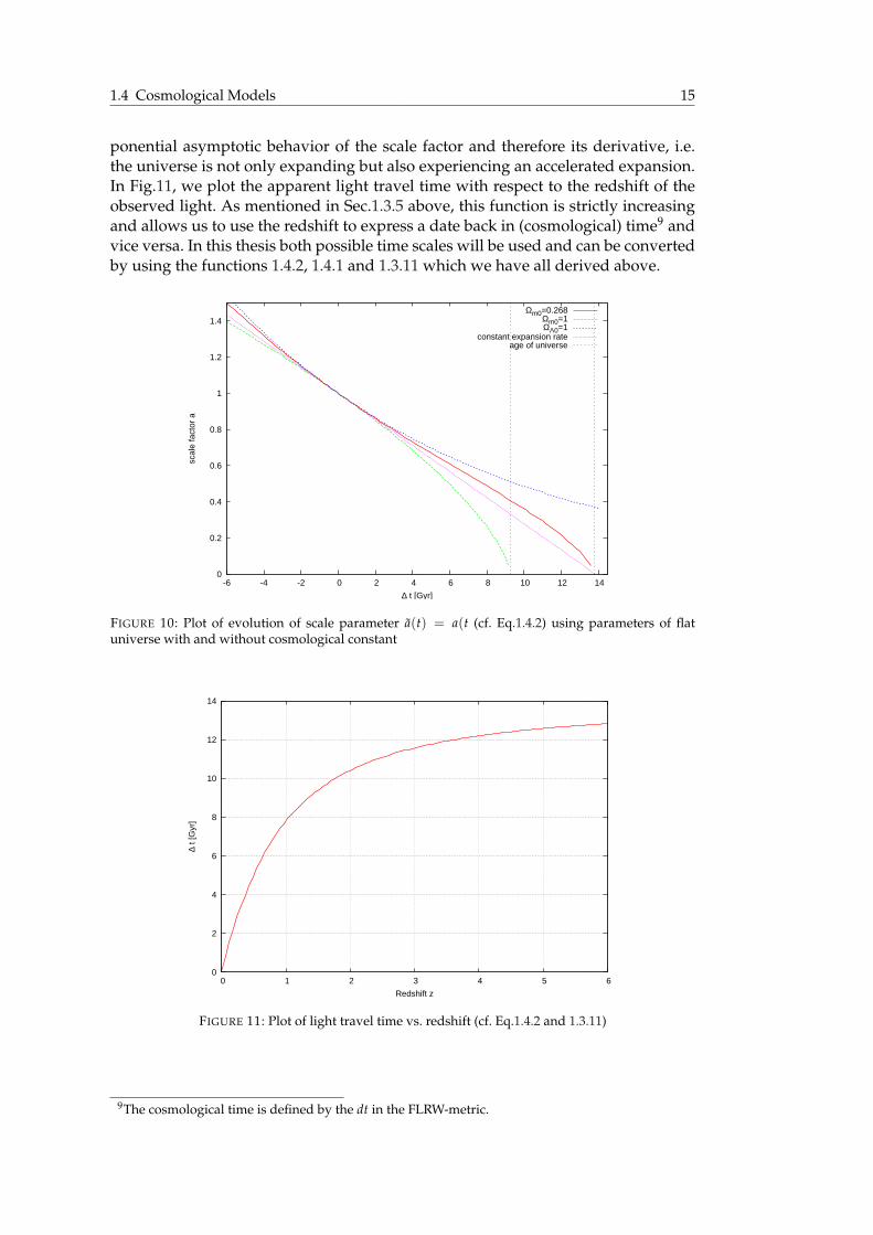
ponential asymptotic behavior of the scale factor and therefore its derivative, i.e.the universe is not only expanding but also experiencing an accelerated expansion.In Fig.11, we plot the apparent light travel time with respect to the redshift of theobserved light. As mentioned in Sec.1.3.5 above, this function is strictly increasingand allows us to use the redshift to express a date back in (cosmological) time9 andvice versa. In this thesis both possible time scales will be used and can be convertedby using the functions 1.4.2, 1.4.1 and 1.3.11 which we have all derived above.
0
0.2
0.4
0.6
0.8
1
1.2
1.4
-6 -4 -2 0 2 4 6 8 10 12 14
scal
e fa
ctor
a
∆ t [Gyr]
Ωm0=0.268Ωm0=1ΩΛ0=1
constant expansion rateage of universe
FIGURE 10: Plot of evolution of scale parameter a(t) = a(t (cf. Eq.1.4.2) using parameters of flatuniverse with and without cosmological constant
0
2
4
6
8
10
12
14
0 1 2 3 4 5 6
∆ t [
Gyr
]
Redshift z
FIGURE 11: Plot of light travel time vs. redshift (cf. Eq.1.4.2 and 1.3.11)
9The cosmological time is defined by the dt in the FLRW-metric.


CHAPTER 2
STRUCTURES IN THE UNIVERSE
In the previous chapter we have discussed, how perturbations of the universe atthe time of last scattering can be observed by analyzing the CMB. They are seen asa isotropic, homogeneous Gaussian random field of mean zero. We will now usethe Comological standard model. Thus, these faint fluctuations in the nearly homo-geneous matter distribution are supposed to become the seeds of all the small andlarge scale structures we can observe today and structure formation is totally basedon this bottom-up process.
Since the goal of this thesis is to compare numerical simulations of structure for-mation processes within the standard model, we briefly discuss in this chapter howstructures in the universe form starting at the growth of the initial perturbations,followed by the collapse of halos and merging processes of increasingly massivehalos. We are going to have then a deeper look at two properties of the alreadycollapsed and virialized halos, namely their density and corresponding potentialprofiles. We hereby present several parameterization models to describe these pro-files.
2.1 Structure Formation & Evolution
As already mentioned in the introduction, the structure formation process in theUniverse is supposed to be hierarchical. Our “initial condition” in the structureformation process is a homogeneous matter distribution with small gaussian fluc-tuations. In the following we will show how to treat the dynamics of such fluctu-ations in the mass density field, first for the linear and ”mildly non-linear” regimeby briefly summarizing the results of linear perturbation theory and, in particular,the Zel’dovich approximation. Thereafter, we look at what happens when a overdenseregion collapses according to the spherical collapse model. Based upon the resultingmodel of bound halos, we derive the statistical evolution of these objects using thePress-Schechter theory and discuss the interactions between the halos leading to the
17

18 Chapter 2 Structures in the Universe
merging processes. Before we start, we have to introduce formally the comovingcoordinate framework and the basics of Newtonian cosmology.
2.1.1 Newtonian cosmology & Comoving coordinates
In general, we would have to work within the framework of general relativity. Un-fortunately, effects of curvature, finite propagation of gravity and similar conse-quences of Eintein’s gravity theory are complicating both the analytical and the nu-merical approaches to study cosmological structures10. Thus, it is preferable to useNewtonian cosmology instead which is governed by Newtonian’s gravity instead.Therefore it has to be argued that such an approach is valid in the cosmologicalcontext. As shown in studies by McCrea and Milne [MM34] and Bonnor [Bon57]Newtonian cosmology coincides with the zero-pressure limits of relativistic cos-mology for the background world model (cf. Friedman’s equations) and its linearperturbation. In a more recent publication , Noh and Hwang [NH06] confirmed thatNewtonian cosmology remain exactly valid on all cosmological scales to the secondorder assuming a zero-pressure, irrotational fluid and ignoring coupling with grav-itational waves. This result allows us to rely on Newtonian gravity in the analysisof even non-linear structure formation. Thus, dynamics of the cosmic fluid can bedescribed using the following ”classic” equations for a static universe:
∇2Φ = 4πGρ (Poisson) (2.1.1)(∂δ
∂t
)+∇ · (ρ~v) = 0 (Mass conservation) (2.1.2)(
∂~v∂t
)+ (~v · ∇)~v = −∇Φ− 1
ρ∇p (Euler) (2.1.3)
As already briefly mentioned in the previous chapter 1 about the metric of the Uni-verse, one convenient coordinate framework is the comoving coordinate system. Itfollows the (uniform) expansion and contraction of the universe. Thus, objects only”floating” in this Hubble flow remain at the same comoving coordinates
~x =~p
a(t)(2.1.4)
while their proper physical coordinates ~p may vary according to the expansion. Wehave already seen in the section about the cosmological redshift, that only observersresting in the comoving framework percieve the Universe to be isotropic.
By scaling the spatial coordinates with respect to the expansion, we also obtainnew ”comoving” forms of quantities depending on the length. They differ from theoriginal form by a factor depending on a(t). In our case, we encounter the followingones:
10Nonetheless, in early works on this topic by e.g. Friedman and Lifschitz the relativistic approachpreceeds the Newtonian one.

2.1 Structure Formation & Evolution 19
velocity The comoving velocity is defined by the time derivative of the comovingdistance given by
~x =d~xdt
=1
a(t)(~v− ~pH(t))
with ~p being the proper position and ~v the proper velocity. The term in thebrackets is hereby the proper perculiar velocity ~vpec, i.e. the physical velocityrelative to the Hubble flow, which is, in contrast to the comoving velocity,observable.
density Since the density is based on the volume and the mass as an intrinsic prop-erty of the mass is not changed by the coordinate transformation, we obtainan additional factor of a3 when we transform the physical density into its co-moving couterpart:
ρcom(~x) = a3(t)ρ(~p/a)
Additionally to the transformation of the spatial coordinates, it is often convinientto introduce also a conformal time τ defined by
dτ =dt
a(t)
This simplifies the line element of the FLRW metric, which becomes:
ds2 = a2(t)[c2dτ − dr2 + f 2
k (r)dω2]Thus, the overall coordinate transformation for spatial and temporal dimensionscombined is thus conformal, i.e. a diffeomorphism which leaves the metric unchangedexcept for an overall factor a(t). This can be used to make the handling of comov-ing equations of motion simplier. An example is to compute the proper peculiarvelocity directly by using only the comoving/conformal quantities:
~vpec =d~xdτ
= ~v− ~pH(t)
Another quantity that can be easily derived by using whole conformal transforma-tion is the comoving distance Dcom [DD09, Ch.26.1]. This is the coordinate distancein the comoving coordinate frame, i.e. in the case of a flat universe the euclideandistance of two points on a three-dimensional spatial hypersurface of constant (cos-mological) time t divided by the scale factor a(t) at that time. Thus for some sourceand observer resting relative to the local Hubble flow the distance is independantfrom t. To compute a distance based on an observation with this measure, we haveto determine the length of the path that a ray of light has passed after its emission.That means, we have to integrate this in comoving coordimates. We thereby substi-tute the spatial comoving coordinates by the conformal time using that ds = 0 inthe light frame11
Dcom =∫ τobserv
τemit
cdτ = c∫ tobserv
temit
dta(t)
= c∫ a(tobserv)
a(temit)
daaa
=c
H0
∫ a(tobserv)
a(temit)
daa2E(a)
(2.1.5)
11Sign convention chosen such that we have decreasing distance towards observer

20 Chapter 2 Structures in the Universe
The whole comoving frame has the great advantage that the equations of the New-tonian cosmology can be rewritten rather easily in order to deal with the dynamicswithin an expanding cosmological system. By expressing the position and velocityin the comoving coordinate frame and the density and the potential still the physi-cal one, the thus get12:
1a2∇
2~xΦ = 4πGρ (Poisson) (2.1.6)(
∂δ
∂t
)~x
+1a∇~x · ((1 + δ)a~x) = 0 (Mass conservation) (2.1.7)(
∂a~x∂t
)~x
+ H(a)~x + (~x · ∇~x)(a~x) = −1a∇~xΦ− 1
aρ∇~x p (Euler) (2.1.8)
where δ is the density contrast with respect to the homogeneous background densityρb and defined by
δ :=δρ
ρb=
ρ(~x, t)− ρb
ρb(2.1.9)
2.1.2 Density perturbation dynamics and Zel’dovich approximation
The determination of the dynamics of small initial perturbations δρ is, in general,very complicated. Thus, we make some assumptions here that simplify the ap-proach significantely:
• The scale of interest, i.e. of the studied inhomogeneities is assumed to be smallcompared to the size of the horizon H−1. As mentioned in the first sectionof this chapter, we then may work to a good approximation, using classicalNewtonian dynamics instead.
• We are working in an Einstein-de Sitter universe, i.e. the cosmological con-stant is ignored in the Poisson equation.
• The universe is dominated by ”cold” matter. Thus we can ignore the special-relativistic fluid mechanics, that would be needed to treat e.g. photons. Addi-tionally, we may ignore the pressure term later on as the Jeans length tends tobe very small for cold matter.
The dynamics are then governed by momentum conservation (Euler equation), bymass conservation (continuity eq.) and by the Poisson equation, to determine thegravitational potential Φ. By taking the divergence of the Euler equation and in-serting it together with the Poisson equation into the total time derivative of thecontinuity equation, obtain the following single equation describing the dynamicsof the density contrast:
δ + 2Hδ = 4πGρbδ +c2
s∇2~xδ
a2 .
12The whole derivation may be found in [Pee93, Ch.5]

2.1 Structure Formation & Evolution 21
To get rid of the spatial gradient in the time evolution, we switch to the Fourierspace and thus to the time-dependent Fourier amplitudes δ(~k, t) that we have al-ready seen in Eq.1.2.3.resulting in
¨δ + 2H ˙δ = (4πGρb −c2
s k2
a2 )δ.
Analysing the limit of a static universe for this equation and therefore loosing the”damping term”, we can see that this results in a simple 2-order ODE, i.e. an oscilla-tor equation. Up to a certain given scale λJ = 2π
k Jof the initial density perturbation
, the evolution is therefore bounded and oscillating. This is the well-known Jeanslength given by
λJ = cs
√π
Gρb
with the first factor being sound speed inside the perturbation. It describes thephysical fact that the gravity of perturbations on small scales is not strong enoughwith respect to the pressure gradient (caused by thermal energy) to keep the parti-cles bound which leads to an oscillation of the density contrast instead of a growth.For CDM this Jeans length tends to vanish, while it remains finite for e.g. neutrinos.Therefore, as already briefly reviewed in Ch.1.4 structure growth can take place on(nearly) all scales for CDM, while it is ruled out on small scales for HDM.
In contrast to the oscillation case, it can be shown that for fluctuations far above theJeans length scale (for which we can now ignore the pressure term), the density con-trast the real-space solution13 for the evolution of δ follow in good approximation
δ(~x, a) =D+(t)D+(ti)
δi(~x) (2.1.10)
where δi is an initial density field at time ti and D+(a) is the linear growth factor givenby [LH01, Eq.2]
D(t) =5Ωm0H2
02
H(t)∫ a
0(t)(aH(a))−3da (2.1.11)
which approaches a(t) in the limit of a matter-dominated universe (usually D+(t)itself is normalized to equal 1 at initial time ti). It can also be shown that by using arelativistic perturbation theory, in a preceding radiation-dominated era this growthfactor is a2 14, but, at the same time, the Jeans length is very large, as the ”speed ofsound” for a relativistic fluid is very high, and nearly the size of the cosmologicalhorizon at that time. This last fact then leads to the shape of matter power spectrumwe already discussed in Ch.1.2.
13or to be more exact, the one growing term14A very detailed prescripton on how to determine D+(t) for many other universes can be found in
[Pee80, Ch.11+]

22 Chapter 2 Structures in the Universe
Unfortunately this way for calculating the growth of the initial (gaussian) fluctua-tions breaks down when the density contrast becomes larger and surpasses unity.One famous approach was therefore proposed by Zel’dovich [Zel70] to extend thistheory into the ”mildly” non-linear regime. It is based on decomposing the matterfluid into an ensemble of particles and to calculate their trajectories to reconstructthe density afterwards. The assumptions thereby are the same that we used for thelinear approach. We start with a decomposition of the initially slightly perturbedparticles from their comoving initial positions ~x. Their physical trajectory is thengiven by
~r(t) = a(t)~x + b(t)~f (~x) (2.1.12)
The second term hereby describes the peculiar motion of those particles and con-tains all the informations about the perturbation. The Jacobian determinant of themapping above provides us with the dynamics of the corresponding density field:
ρ = ρ0det−1[
∂ri
∂xi
]= ρ0 det−1
[a(t)δij + b(t)
∂ fi
∂xj
]where ρ0 is the mean density at present time. We can now explicitely compute thedeterminant, if the matrix within it is diagonalizable with eigenvectors λi(~x). Ifwe additionally use, that for non-relativistic matter the mean density evolves like∼ ρ0a−3(t), we get for the density contrast at an arbitrary time t:
δ =[(1 +
ba
λ1)(1 +ba
λ2)(1 +ba
λ3)]−1
− 1
≈ −ba(λ1 + λ2 + λ3) = −b
a∇~x~f
Comparing this result with the linear perturbation theory, gives us finally:
δ = −D(t)∇~x~f (2.1.13)
with D(t) being the linear growth factor.
Using Eq.2.1.12 we can also calculate the comoving velocity ~x (which automaticallyfulfills the continuity equation Eq.2.1.7):
~x =~ra− a
a2~r =1a(a~x + b f − a
a(a~x + b~f ))
= ∂t(ba)~f ⇒ ~x = D(t)~f (~x) (2.1.14)
While the Zel’dovich approximation allows us to follow the evolution into the non-linear regime, it no longer plays an important role as today systems with evenhighly non-linear density distributions can be studied by using numerical simula-tions. But as we will see in Ch.3.3 some of the results we got remain every importantfor constructing initial conditions used in these simulations.

2.1 Structure Formation & Evolution 23
2.1.3 Spherical Collapse Model
After having discussed how perturbations grow, we will now focus on their col-lapse. As an approximation, we will start assuming that initial fluctuations result insmall, uniform, spherically symmetric overdense regions. Due to Friedman’s equa-tion 1.3.6, the evolution of the scale factor can be written as:
dadt
= H(t) · a = H0
[1 + Ωm0(
1a− 1) + ΩΛ0(a2 − 1)
] 12
=:H0
f (a)(2.1.15)
As seen, linear perturbation theory provides the growth factor for the linear densityfluctuations. Rewriting Eq.2.1.11 using f (a) as defined in the evolution equationabove, we obtain
D(a) =5Ωm0
2a f (a)
∫ a
0f 3(a)da
As mentioned before, this results, in the case of a flat universe (Ωm = 1, ΩΛ = 0),in D(a) = a which holds for universes with arbitrary Ωm and ΩΛ for small a. Theevolution of the radius of these spherical regions with an initial radius Ri and initialoverdensity ∆i = 1 + δi (relative to the background ρb,i) can easily be derived bylooking at the energy equation of the surface given by:
E =12
(drdt
)2
− GMr− Λr2
6(2.1.16)
where M = M(ri) = 43 πR3
i ρb,i∆i is the enclosed mass. Substituting r by the relativeradius with respect to the initial one s = r
r i and assuming conservation of energy(i.e. E = Ei) and that ds
dt |si = 0, we can transform this equation (in analogy to theevolution of a in Eq.2.1.15) into:
(dsdt
)2
= H(ai)2[
1 + Ωm(ai)(1s− 1) + ΩΛ(ai)(s2 − 1)
]=:
H(ai)g(s)
(2.1.17)
The turn-around radius is reached when the differential vanishes in Eq.2.1.17 (be-sides at the solution si = 1 given by the initial conditions). Thus, we get a cubicequation of the form:
AC
s3ta −
BC︸︷︷︸=:κ
sta + 1 = 0 (2.1.18)
where A = ΩΛ(ai), B = 1−Ωm(ai)∆i −ΩΛ(ai) and C = ΩΛ(ai). Due to its formthere exist a minimal value for κ so that we get a real-value solution. Comparingthe coefficients of this cubic equation with those in Eq. 2.1.16, it can be seen, thatthe initial sphere has to have a given minimal overdensity ∆i,min (depending on thecosmological parameters) in order to collapse. Besides, this limit ceases to exist inthe limit of a flat, critical CDM universe with a vanishing cosmological constant asthe cubical equation becomes a linear one.

24 Chapter 2 Structures in the Universe
Fulfilling these constraints on the initial conditions, the solution of the cubic equa-tion that is physically sensible in both the case of arbitrary cosmological parametersand the limit of small Λ finally is given by:
Rta =2√3
(BA
) 12
cos(arccos(α)
3− 2
3π)Ri (2.1.19)
where α = − 9A12 C
2B32
. Regarding that the last factor can be approximated by cos(. . . ) ≈α3 in the limit of small A, it is easy to see that the limit of this solution for a criticaluniverse is in fact as expected sta = C/B.
The scale factor ata at turn-around can now finally be obtained by separating thevariables in the two equations of evolution 2.1.15 and 2.1.17 and integrating in eachof them both sides. Hence we get:
∫ ata
0f (a)da = H0t ∧
∫ sta
0f (s)ds = H(ai)t
⇒∫ ata
0f (a)da =
H0
H(ai)
∫ sta
0f (s)ds (2.1.20)
which can be solved at least numerically using the general solution of sta that hasbeen found earlier.
2.1.4 Virialization
After passing the point of the turn-around, the perturbation is bound to collapse,this collapse will stop when the perturbation reaches the state of virial equilibriumdefined by the following theorem:
Theorem 2.1.1 (Virial theorem [Col78, Ch.1] ). If a system is in a steady state and gov-erned by a particle-particle interaction based on a potential of the form V(r) = αrn, thenyields
2〈T〉 − n〈VTOT〉 = 0 (2.1.21)
where 〈T〉 and 〈VTOT〉 are the time averages of the total kinetic and potential energy.
In our case, the dynamics of the particles are governed by gravitation and darkenergy. Thus n = −1 and n = 2 and Eq. 2.1.21 becomes
〈T〉 = −12〈VTOT,Grav〉+ 〈VTOT,Λ〉 (2.1.22)
Using this relation, it has been shown in [LLPR91] that the virial radius Rvir of thehalo, i.e. the radius of the virialized spherical region is approximately
Rvir ≈1− η
2
2− η2
Rta (2.1.23)

2.1 Structure Formation & Evolution 25
where Rta is the turn-around radius that we have determined in the preceding sec-tion and η is proportional to the cosmological constant Λ. Thus, in the case of ayoung, matter-dominated universe the virial radius is half the size of the radius atturn-around and in the case of an older, dark energy-dominated universe, the virialradius compared to the turn-around radius becomes smaller. This reduction is ex-pected due to the additional ”repulsive” potential of the dark energy in Eq. 2.1.22.
Given the results of the collapse model and the virial radius, the density or, to bemore precise, the overdensity ∆c relative to the critical density inside the virializedhalo can finally be determined. Since the background density scales like a3 whilethe halo density scales like R3, we obtain
∆c = Ω(ac)(
ac
Rvir
)3
(2.1.24)
where ac is the expansion factor at the collapse time of the halo. The collapse is ex-pected to happen at twice of ata, for which we have found Eq.2.1.20.
To simplify this formula, we assume the same initial conditions as in [Pee84]/[ECF96,Appendix A]. Then it can be fitted with the following function [BN98]:
∆c = 18π2 + 82x− 39x2 (2.1.25)
where x = Ω(a)− 1.
2.1.5 Press-Schechter Theory & Mergers
As seen, the result of the spherical collapses are gravitationally bound halos. ThePress-Schechter formalism is now an analytical attempt to estimate the mass func-tion of such objects. The idea behind it, is to calculate the probability of meetingthe requirements for spherical collapse, i.e. having a mean density above ρc, in re-gions of a certain mass M. This is done by filtering the density contrast field δ(~x) onthe scale R(M) (cf. Eq.1.2.4) which corresponds to the radius of an homogeneouscritical sphere of this mass M. For a Gaussian random field, we have then a proba-bility p(δR(~x), a) to find a specific filtered density contrast δR at position ~x and forscale factor a given by the normal distribution N (0, (σRD+(a))2). Since we are inthe following interested in excluding the presence of halos more massive than M,we need to determine instead the probability of having a filtered density contrastδR at ~x, which never exceeds the critical density at any larger scale R. Eq. 2.1.26 thusmust be correct as follows15
p(δR(~x), a) =1√
2π(σRD+(a))2
[exp(− δ2
R(~x)2(σRD+(a))2 )− exp(− (2δc − δR(~x))2
2(σRD+(a))2 )]
(2.1.26)
15We hereby simply use the absorbing barrier argument for the ”random walk” of δ′R for R′ approach-ing R from above. This gives the second term.

26 Chapter 2 Structures in the Universe
By integrating over the filtered density contrast up to δc, we thus obtain the proba-bility to find a halo at ~x which has a mass M or higher:
F(M, a) = 1−∫ ∞
δc
dδR p(δR, a)︸ ︷︷ ︸=:P(σR,a)
= erfc(δR(~x)√
2σRD+(a)) (2.1.27)
with the complementary error function
erfc(x) =2√π
∫ ∞
xexp(−t2)dt (2.1.28)
The distribution of halos over mass M is now given by ∂F(M, a)/∂M which we canfinally use to obtain the number density of halos of mass within [M, M + dM] bydeviding the result by the mean volume occupied by M:
N(M, a)dM =√
2π
ρbρcdMσRD+(a)M
dσR
dMexp(− δ2
R(~x)2(σRD+(a))2 )
It is remarkable, that this result already describes the results found in numericalsimulations quite well. These results can also be used to derive a theory aboutmerging events. Following [LC93], this is accomplished by using Eq.2.1.27 to firstcalculate the probability to reach the critical density at a given time/scale factor a1for a given σR,1 under the condition of having reached the critical density at a sec-ond time with a different σR,2. By substituting σR by the corresponding masses andtaking the limit of an infinitesimal time step, we obtain the probability that a haloof mass M1 reaches mass M2 = M1 + ∆M by (instantly) accreting a second halowithin the time interval [t, t + dt]:
d2 pM
d(ln ∆M)dt(M2, t|M1, t) =
σR,2
d(ln ∆M)
∣∣∣∣dD+(a)dt
∣∣∣∣ −d2 ∂P(σR,2,a)∂S
dσR,2dD+(a)(σR,2, D+(a)|σR,1, D+(a))
To avoid unnecessary distraction we skip to write out the final form by substitut-ing the derivatives with their results. It can be found together with other deduc-tions (e.g. of the halo-survival time) in the original paper cited before. As has beenalso shown in the paper, the merger rates for halos of mass ∆M M1 dominate,but the mass accretion is mainly caused by mergers with more massive halos. Themerger history can be then graphically illustrated by drawing a so-called mergertree as shown in Fig.12. In a nutshell, this deduction is an analytical attempt to char-acterize the hierarchical structure formation process, that we also observe in oursimulations by the infall of satellites into our main halo16. This is also reflected inthe increases of the Halo mass of the Galaxy halos in the simulations as plottedin Fig.13, whose curves are part-wise very monotonic, but also show huge sponta-neous increases like the one occured for Gal1 before z = 1 as major mergers takeplace
16see e.g. major merger in Fig.38

2.1 Structure Formation & Evolution 27
FIGURE 12: Schematic representation of the accredition history of a halo [LC93, Fig.6]
0
2e+11
4e+11
6e+11
8e+11
1e+12
1.2e+12
1.4e+12
1.6e+12
0 2 4 6 8 10 12 14
MH
alo
[MO•
]
age of universe [Gyr]
Gal0Gal1Gal3z=1
FIGURE 13: Plot of mass evolution of three galaxy halos (in pure DM simulations)
2.1.6 Interaction: Dynamical friction & Tidal Stripping
While we presented the predicted rate of halo mergers/accretion, we have to dis-cuss these processes of interaction between an infalling satellite and a host halo.Two effects are thereby essential in a collisionless system, namely Dynamical frictionand Tidal stripping.
Dynamical friction, which first discussed in detail by Chandrasekhar [Cha43], causes

28 Chapter 2 Structures in the Universe
an momentum and kinetic energy loss for infalling halos such that they sink furtherinto the virialized host halo after their first infall. This is caused by the gravitationalinteraction of the infalling halo with the matter of the host halo. While passing thehost halo the infalling satellite causes a gravitational wake behind it, i.e. an local in-crease of the density which pulls the satellite in opposite direction to its velocity andthus slowing it down. This deceleration thereby depends on both the mass densityof the (slower) particles in the halo, the mass of the satellite and the inverse of thesquared velocity of the orbiting satellite in the restframe of the host halo. The re-sulting energy loss is illustrated in Fig.14 by plotting the total energy (i.e. kinetic +potential energy) per mass unit over time.
0.2
0.4
0.6
0.8
1
1.2
1.4
0 0.1 0.2 0.3 0.4 0.5 0.6 0.7 0.8 0.9 1-0.0052
-0.005
-0.0048
-0.0046
-0.0044
-0.0042
-0.004
-0.0038
-0.0036
r/R
vir
spec
ific
tota
l ene
rgy
redshift z
Gal0 - Group 225 (rel.) Distance to Galaxy specific total Energy
distance to centerenergy
FIGURE 14: Plot of specific energy over time for a satellite
The second, important effect is the tidal stripping (cf. e.g. [RWE+06]) and causesthe satellite to lose matter to the host halo. It is induced by the gradient of the grav-itational potential of the host halo. Thus, the part of the infalling halo closer to thehost halo is thereby exposed to a stronger gravitational pull than the opposite side,which leads to an radial distortion of the halo up to the point where the outer-most particles are stripped from the surfaces of the satellite facing and opposingthe host halo resulting in characteristic tidal tails trailing or leading the satellite’spath. The radius at which the particles finally become unbound to the satellite isthereby called tidal radius. If a satellite passes a region of a very large gravitationalgradient, i.e. close to the center of the host halo, or if its particles are already onlyloosely bounded, this effect may become so large that the whole satellite is com-pletely disrupted leaving a so-called tidal stream behind. Fig.15 shows this processfor a satellite in our simulation. The particles belonging to the satellites at the firstredshift have been therefore marked in the sequence of time snapshots showing thedevelopment of the tidal tails due to tidal stripping.

2.2 Density/Potential profiles 29
FIGURE 15: Snapshots of Gal0 illustrating tidal stripping at an infalling satellite
2.2 Density/Potential profiles
One important characteristic of these matter halos is its density and its correspond-ing potential profile. While there is no model that explains the halo structure analyt-ically in detail, there exist several profiles, partially obtained by simplified physicalmodels (e.g. by assuming isothermal conditions) and partially motivated by pro-files observed in numerical simulations. In the following section, we will presentsome of the most common profiles, that we chose to use in our analysis.
It should be hereby noted that we will work here in a static frame at a = 1, i.e. usingthe static equations of Newtonian cosmology (Eq.2.1.1-2.1.3). Nonetheless, all theresulting formulas for the profiles can be easily rewritten for the comoving frame bysimply replacing all quantities, i.e. positions, scale factors and densities, with theircomoving counterparts. All contributions of a(t) automatically cancel out and weobtain the expansion-independent comoving density profiles that we than can usefor our fittings in the analysis. The potential profiles are then also invariant exceptfor a prefactor a(t) by switching to the fitted comoving parameters and distances.

30 Chapter 2 Structures in the Universe
2.2.1 Singular Isothermal Sphere Model
A rather simple analytic model for the density profile is the so-called singular isother-mal sphere. Therefore we assume a spherically symmetric, self-gravitating systemof non-interacting particles in hydrostatic equilibrium at temperature T. Thus, thefirst equation describing this system is the Navier-Stokes equation for vanishing vis-cosities, also known as the Euler Eq., that we have already seen for a expandinguniverse in Eq. 2.1.8. The potential gradient, or to be more exact, the the resultinggravitational force (per unit volume) f (r) = −∇~rΦ/ρ with r being the distancefrom the center of the sphere is thereby given by
f = −GM(r)r2 ρ = −G
r2
∫ r
04πρ(r)r2dr (2.2.1)
The equation can be simplified by taking the spherical symmetry into account.Hence, we get:
⇒ 1ρ(r)
dpdr
= −Gr
2 ∫ r
04πρ(r)r2dr (2.2.2)
Furthermore, for the pressure p yields the equation of state for an ideal gas:
p =kTm︸︷︷︸
=:σ2
ρ (2.2.3)
where m is the mass of each particle of the system. By inserting this into Eq. 2.2.2,we obtain:
⇒ σr2 1ρ(r)
dρ(r)dr
= −ρG∫ r
04πρ(r)r2dr
⇒ ddr
(r2 d(ln(ρ(r))
dr
)= −4πG
σ2 r2ρ(r)
This second-order differential equation for ρ has at least two solutions. The singularone which we want to use is thereby:
ρSIS(r) := ρsing(r) =σ2
2πGr2 (2.2.4)
One major flaw of this model is the assumption of a constant temperature through-out the sphere, which would necessarily lead to an evaporation of particles at thesurface. The model can therefore be used at best as an approximation in the innerparts of a halo. We will nevertheless test it against our simulation results and con-sider it as possible valid model to describe the density and the potential profile. Todo so, we now still have to determine the corresponding potential. In general, thisis done by solving the Poisson equation, but since we are in a spherical symmetric

2.2 Density/Potential profiles 31
system, Eq.2.1.6 can be simplified to become (in spherical coordinates)17
1r2
∂
∂r
(r2 ∂
∂r
)Φ = 4πGρ(r) (2.2.5)
and it can be easily shown (cf. e.g. [BT87, Ch.2.1]) that the solutions of this second-order partial differential equation does also depend only on the radius r and isgiven by
Φ(r) = −GM(r)r− 4πG
∫ ∞
rρ(r)rdr (2.2.6)
where
M(r) = 4π∫ r
0r2ρ(r)dr (2.2.7)
is the so-called mass profile function, i.e. it returns the mass enclosed in a sphere ofradius r around the origin.
Thus, we have to determine in two steps first M(r) and then Φ(r):
MSIS(r) = 4π∫ r
0r2ρSIS(r)dr = 4π
∫ r
0
σ2
2πGdr =
2σ2
Gr
⇒ ΦSIS(r) = −GMSIS(r)r
− 4πG∫ ∞
rρSIS(r)rdr
= −2σ2 − 4πG∫ ∞
r
σ2
2πGrdr = (−2)σ2(1 + [log(r)]∞r )
Unfortunately, the mass profile doesn’t converge for large r, i.e. the total mass isinfinite and the same is true for the potential. An easy way to fix this, is to introducean cut-off at an arbitrary large, but still finite radius. By doing so, we get a sensible,finite potential function for all r < rcutoff, that still properly solves the PDE given inEq.2.2.5:
ΦSIS(r) = (−2)σ2(1 + [log(r)]Rcutoffr ) = 2σ2 log(r) + C (2.2.8)
where we combined all the constant parts into C. Since we henceforth are going todetermine only differences in the potential, we don’t need to care further about itsactual value.
2.2.2 Zhao’s (α, β, γ)-Models
The (α, β, γ)-Models proposed by Hernquist [Her90] and Zhao [Zha96] is not justa simple model, but instead an attempt to unify many of the formerly proposedparticular models in a general family of models using five parameters. Henceforthuntil further notice we will assume to have spherically symmetric values. This may
17We can and will henceforth in this section neglect the cosmological constant as the potential in thishigh-density regions are mainly governed by the gravitational part. We also work at a = 1

32 Chapter 2 Structures in the Universe
not be true for every studied halo, especially not for the larger main halos, but itshould provide a good enough approximation on the one side, as well as a desiredsimplification of the analytical models on the other. Taking this into account, Zhao’sfamily of models is parameterized by the three variables α,β and γ and two addi-tional scale parameters Rs and ρ0. The (radial) mass distribution is then definedby
ρ(r) = ρ0
(r
Rs
)−γ[
1 +(
rRs
) 1α
]−α(β−γ)
(2.2.9)
We easily notice, that the SIS model as given by Eq.2.2.4 is actually a member ofthis family, since it can be obtained by setting (α, β, γ) = (1, 2, 2)) and substitutingthe scaling factors by σ = RS
√ρ0. We will now discuss two further members of this
family, that are at the moment very popular to describe halo density profiles foundin numerical simulations and will therefore also be used in this thesis.
Navarro-Frenk-White profile
In 1995 Navarro, Frenck and White argued that while Halo profiles are approxi-mately isothermal over a large range in radii, the results of their DM simulationsshow that the profiles are in fact significantely shallower in the inner parts andsteeper than r−2 in the outer regions [NFW96]. To fit the numerical results betterthey presented a ”universal” model that was more consistant with their data, theNavarro-Frenk-White (NFW) profile.
ρNFW(r) =ρ0(
rRs
) [1 +
(r
Rs
)]2 (2.2.10)
As done for the SIS potential, we are now going to determine the potential functionby performing the same two steps. Hence we get
MNFW(r) = 4π∫ r
0r2ρNFW(r)dr = 4πρ0R3
s
∫ r
0
r
[Rs + r]2dr
= 4πρ0R3s
(log(
Rs + rRs
)− rRs + r
)⇒ ΦNFW(r) = −GMNFW(r)
r− 4πG
∫ ∞
rρNFW(r)rdr
= −4πGρ0R3s
(1r
log(Rs + r
Rs)− 1
Rs + r
)− 4πGρ0R3
s
∫ ∞
r[Rs + r]−2 dr
= −4πGρ0R3s
(1r
log(Rs + r
Rs)− 1
Rs + r+[
1Rs + r
]∞
r
)
⇒ ΦNFW(r) = −4πGρ0R3s
log( Rs+rRs
)r
(2.2.11)

2.2 Density/Potential profiles 33
It is maybe noteworthy, that the total mass is, in contrast to the SIS model, finite andthe potential has an upper bound.
Generalized Navarro-Frenk-White profile
As pointed out by Jing and Suto [JS00] density profiles of dark matter halos, espe-cially the inner slopes, are not so universal as Navarro, White and Frenck assumedfor their model. Therefore they proposed a generalization of the NFW model thathas the ability to model inner logartihmic slopes with arbitrary constant inclines.This leads to the following formula describing this profiles:
ρGNFW(r) =ρ0(
rRs
)γ [1 +
(r
Rs
)](3−γ) (2.2.12)
And once again, we obtain the mass profile and the potential function by usingEq.2.2.6 and 2.2.7:
MGNFW(r) = 4π∫ r
0r2ρGNFW(r)dr = 4πρ0R3
s
∫ r
0
r2
rγ [Rs + r](3−γ) dr
ΦGNFW(r) = −GMGNFW(r)r
− 4πG∫ ∞
rρGNFW(r)rdr
⇒ ΦGNFW(r) = −4πGρ f00(r
Rs)2 (2.2.13)
where f00 is given by
f00 =B(χ, c0 − q0, q0)B(c0 − q0, q0)
χc0−q0(1− χ)q0+
B(1− χ; c0 − p0, p0)B(c0 − p0, p0)χp0(1− χ)c0−p0
with B(·; ·, ·) beeing the (incomplete) Beta-function and χ = r/(r + Rs), c0 = β− γ,q0 = β− 3, p0 = 2− γ, ρ = ρ0(r/Rs)−γ(1 + r/Rs)−c0
2.2.3 PoLLS / Einasto model
Another possible approach to group particular models into more general familieshas been presented by Cardone et al.[CPT05]. They thereby started to compare par-ticular models by looking at the logarithmic slope of the density profile, which isdefined as
α(r) :=d log ρ
d log r(2.2.14)

34 Chapter 2 Structures in the Universe
and proposed to use the following function to get a sensible parameterization of α,that is general enough to fit the majority of the popular models
α(r) = −β1 + a(r/Rs)1 + b(r/Rs)
(r
Rs
)γ
(2.2.15)
where Rs is again a scaling factor for the radial distance r and a,b,β and γ are theparameters of this family of slope functions18. The corresponding density profilescan then be obtained by solving Eq.2.2.14 for ρ, i.e. integrating Eq.2.2.15 with respectto r:
ρ(r) = exp(∫
α(r)r
dr) (2.2.16)
While this is possible for an arbitrary choice for the parameter values, it can beshown that the mass profile (Eq.2.2.7) can only be expressed analytically for thefollowing two classes19
• γ = 0 and b 6= 0:
α(r) = −β1 + a(r/Rs)1 + (r/Rs)
(2.2.17)
where we have w.l.o.g. set b = 1 and rescaled the remaining three parametersaccordingly,
• a = b = 0:
αPoLLS(r) := −β
(r
Rs
)γ
(2.2.18)
We have to consider this, since we are also interested in the potential profiles of thehalos later on. Comparing the resulting profiles of the first case, we see that thisis just a subset of Zhao’s family of models, to be more precisely, a subset of the(1, βZhao, γZhao)-models20. The case of a = b = 0 provides us with a class of den-sity profiles with a logarithmic slope following a power law. They will be referredto as power-law logarithmic slope (PoLLS) models. The table Tab.2 shows models in-cluding N04 which is a PoLLS model with parameters determined by Navarro etal. [NHP+04].
Studies of simulated halos performed by Merritt et al. on halos generated by gravi-tational clustering in ΛCDM simulations and by isolated spherical collapse [MGM+06]have shown that the PoLLS models seem to provide in general a better approxima-tion of the real density halos than the other models that we have presented before.
18In fact, Cordone et al. proposed a slope function where the nominator and denominator also containthe squared term of r and therefore needed to more parameters, but, as also mentioned in thepaper, the simplified function is already sufficient to deduce most of the frequently models
19This doesn’t rule out, that there are not particular models like the SIS that also contain analyticalmass profiles, but they form no additional whole class of models satisfying this property.
20The more general models (i.e. with αZhao 6= 1) were lost by not including the second order terms inthe nominator and denominator of the slope function in Eq.2.2.15.

2.2 Density/Potential profiles 35
Model dens. profile ρ a b β γ
SIS ∼ r−2 0 0 2 0NFW ∼ r−1(1 + r)−2 3 1 1 0GNFW ∼ r−γZhao(1 + r)γZhao−3 3/γZhao 1 γZhao 0PoLLS ∼ exp(−γ−1[βrγ − 1]) 0 0 * *N04 ∼ exp(r0.17 − 1) 0 0 2 0.17
TABLE 2: Spherical density profiles for some selected popular galaxy models. The models of the uppergroup except the SIS model belong to the class of models defined by the slope in Eq.2.2.17, while theslope of the lower two models fulfills Eq. 2.2.18.
We also confirmed this (cf. 5) and thus also prefer to use these PoLLS profiles whenwe are going to fit our found density profiles and extrapolate the orbits of the satel-lites. Therefore we again have to determine the mass and potential profile.
First we have to derive the density function itself as described in Eq.2.2.16:
ρPoLLS(r) = exp(− β
2Rγs
∫2rγ−1dr) = exp(− β
2Rγs
2γ
[rγ + C])
where C is the integration constant, which gives us a scaling factor ρ−2 := exp(− (C+1)βRsγ )
in front of the exponential function. We also replace the scale radius Rs by a newscale parameter R−2 defined by the radius, at which the value of the slope of thePoLLS model equals the one of the SIS model, i.e. αPoLLS(R−2) = −2. Since αPoLLS(r)is strictly increasing for positive r, R−2 = (2/β)1/γ Rs is well-defined, the newlydefined scaling factor ρ−2 is just the density at this radius and the formula for thedensity profile thus simply becomes
ρPoLLS(r) = ρ−2 exp(− 2γ
[(r
R−2
)γ
− 1]) (2.2.19)
Using this density function in Eq.2.2.7 gives us the mass function:
MPoLLS(r) = 4π∫ r
0r2ρPoLLS(r)dr
= 4πρ−2R3−2 exp(
2γ
)∫ r/R−2
0(
rR−2
)2 exp(− 2γ
(r
R−2
)γ
)d(r/R−2)
ξ := 2γ ( r
R−2)γ
= 2πρ−2R3−2 exp(
2γ
)(γ
2
)3/γ−1
·[(∫ ∞
0exp(−ξ)ξ3/γ−1dξ)− (
∫ ∞
2γ (r/R−2)γ
exp(−ξ)ξ3/γ−1dξ)
]
The integrals on the right hand are the usual Γ and upper incomplete Γ function,which converge absolutely for Re(3/γ) > 0 and therefore γ > 0. Thus, the above

36 Chapter 2 Structures in the Universe
formula can be simply written as:
MPoLLS(r) = 2πρ−2R3−2 exp(
2γ
)(γ
2
)3/γ−1[
Γ(3/γ)− Γ(3/γ,2γ
(r/R−2)γ)]
(2.2.20)
By taking MPoLLS(r) to the limit of large r, we also notice that the total mass for thismodel is also finite and is given by
MPoLLStot = lim
r→∞MPoLLS(r) = 2πρ−2R3
−2 exp(2γ
)(γ
2
)3/γ−1Γ(3/γ) (2.2.21)
By applying the same method of handling the integral on the second summand inEq.2.2.6, we finally get for the corresponding potential profile:
ΦPoLLS(r) = −GMPoLLS(r)r
− 4πG∫ ∞
rρPoLLS(r)rdr
= − GMPoLLStot
R−2Γ(3/γ)
[R−2
r
(Γ(3/γ)− Γ(3/γ, 2/γ · ( r
R−2)γ))
+(
2γ
) 1γ
Γ(2/γ, 2/γ · ( rR−2
)γ)
](2.2.22)
One special case of the PoLLS model is the so-called N04 model, which has beenproposed by Navarro et al.[NHP+04]. It has β fixed at 2, which results in R−2 = Rsand a small exponent of 0.14.
2.2.4 Comparison
Now, after having finished our collection of halo models, we are now going tobriefly compare their properties, or to be more exact, point out the differences be-tween the models. Fig.16 compares herefore the different logarithmic slope. For themore general models, i.e. GNFW and PoLLS we picked two representatives whoseparameters represent best the results found in the simulation. For the inner core ofa halo, the SIS profile already has the steepest profile that is still physically possible,since steeper density profiles would lead to an infinite mass in the center. Thereforethis model tends to overestimate the density not only in the outer but also in theinner parts of the halo.
The NFW profile has fixed values for the inner and outer slope, i.e. -1 and -3 and theonly free parameter in the logarithmic slope is therefore the position of the transi-tion between these two slopes given by Rs. As can be also seen in this comparisiondoes the generalized NFW hereby only differ from the NFW in its ability to adjustthe inner slope according to the fitting data.
Lastly, the PoLLS provide the possibility to adapt a profile to inner slopes by ad-justing the offset β and, in contrast to the models presented ealier, also to differentouter slope by varying the exponent γ. This allows us to get better fits at the outerrim of the halo, if the actual density does not match the logarithmic slope of −2 or
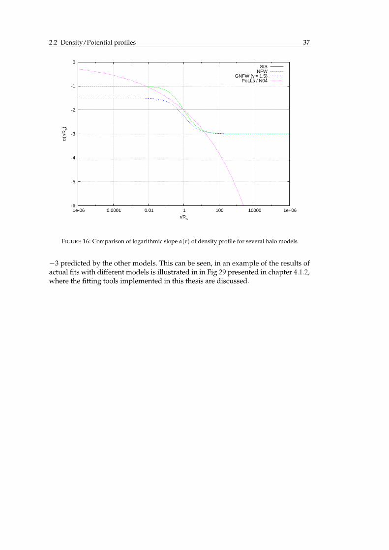
2.2 Density/Potential profiles 37
-6
-5
-4
-3
-2
-1
0
1e-06 0.0001 0.01 1 100 10000 1e+06
α(r/
Rs)
r/Rs
SISNFW
GNFW (γ = 1.5)PoLLs / N04
FIGURE 16: Comparison of logarithmic slope α(r) of density profile for several halo models
−3 predicted by the other models. This can be seen, in an example of the results ofactual fits with different models is illustrated in in Fig.29 presented in chapter 4.1.2,where the fitting tools implemented in this thesis are discussed.


CHAPTER 3
NUMERICAL SIMULATIONS
As it has been noted in Ch.2, the formation history of large and complex objectslike galaxies or galaxy clusters is based on the accretion of thousands of smallerobjects and each of these events is then the source of shocks, turbulences and radi-ation which has further influence on the formation process. Thus, we are in generalconfronted with highly non-linear dynamics.
A way to tackle this problem is to resort to numerical simulations. The universeor, more precisely, the part of it we want to simulate for this purpose, has to bediscretized such that we can handle it within the limit of numerics. We will dis-cuss what this really means in the next section . Then it is possible to simulate theformation process on this discrete representation and to verify the underlying cos-mological model by comparing the results to structures that are observed by as-tronomers today. As every numerical solution, it can always be just an approxima-tion since the limits of a feasible simulation like computational time and memoryput strict constraints on the resolution and volume of the simulated space. Espe-cially in cosmology the trade-off is often hard to choose, since, on one hand, thesimulated volume has to be large enough to not only contain the structures that weare planning to study itself, but also to minimize boundary effects and present a rea-sonable environment for the formation process we want to study. Thus, typical sizesof the simulated volume are a megaparsec scale to simulate an individual galaxy,ten to hundred megaparsecs 21 for galaxy populations and even several hundredmegaparsecs if it comes to simulate a galaxy cluster population. On the other hand,a high resolution is needed to resolve the objects of interest at a certain requiredlevel of detail. Even in the high resolution region of the simulation performed forthis thesis, the side length of the initial cell was about 20 kpc 22 containing a darkmatter mass of 106M and stellar and gas mass scales even less well resolved byan order of magnitude. Some aspects of the dynamics that have to be taken intoaccount in the simulation show up at a relatively small scale, i.e. star formation
21e.g. in the case of the simulations for this thesis the volume had a side length of 90 Mpc (in comovingcoordinates)
22if not mentioned otherwise, all distances will be given with respect to a comoving system
39

40 Chapter 3 Numerical simulations
and supernova events. As we have to deal with length and mass scales a few or-ders of magnitude above the scales of these phenomena, they are not modelled asthe rather single deterministic processes in stellar evolution. But as random eventdepending on the attributes of the cell (and environment) and based on observedstatistics. This stochastical treatment sets further limits on how the influence/feed-back of these events on the formation process can be taken into account.
The following sections will first focus on the different methods to model a discreterepresentation of the universe that then can be used in the simulation. We are goingto present a brief summary of the development in cosmological simulation tech-niques. This is done to outline the origins of the techniques used in the specificsimulation codes, namely pkdGrav and Gasoline, that have been used to produce thesimulation results analyzed in this thesis and will be discuss in the next to last partof this chapter. The final section is reserved to present the actual simulations for thisthesis and their parameters.
3.1 Discretization techniques
As mentioned, the chains of numerics force us to model the universe in a way thatit can be stored in a memory of finite size and be simulated in a finite number of cal-culation steps. But the content of the universe seems to be per se a rather continuousfluid with all attributes being some kind of tensor fields defined at (nearly) everypoint in space-time. There are now several ways to ”fix” this non-storable continu-ity, which we will introduce now. We will thereby handle space and time separately.This is possible since we have seen in Ch.1 that spacetime can be decomposed intospatial hypersurfaces.
3.1.1 Space
grid-based techniques The grid-based techniques work with a discretization of thespace in the simulated volume. The space is thereby partitioned in cells andvalues of the physical properties are then picked for all points in each cell ina certain way. The most simple way to do this is called central difference schemewhere the quantities only represented by the values derived by a pointwiseapproximation at the grid centers (first-order approximation) and derivativesare obtained by a finite-difference representation, i.e. in a three-dimensionalrectangular grid where each cell is identified by the triple (i, j, k) and f(i,j,k) isthe centered value of quantity at the correspondending cell, a second-orderrepresentation is simply given by
∂i f(i,j,k) = −f(i+1,j,k) − f(i−1,j,k)
2h(3.1.1)
where h is the grid spacing.
More modern approaches on representing fields in the discrete space use higher-order schemes, i.e. take neighboring cells into account for reconstruction of

3.1 Discretization techniques 41
the property values for an arbitrary point inside a cell. Some examples willbe briefly introduced later on (cf. Section 3.2.2 / Fig.23). In any way, this ap-proach provides a quite effective handling of local properties derived by (par-tial) differential equations like e.g. gravitational forces by Poisson equation orhydrodynamical quantities by the corresponding hydrodynamical equations,that we will encounter e.g. in cosmological simulations with pure cold darkand baryonic matter. But one major disadvantage of this discretization tech-nique is the limited spatial resolution.
particle-based techniques The other method is to sample the phase-space densityof the matter filling the universe with a set of tracer particles each markinga small variable parcel of fluid and therefore small but finite mass. The dy-namics of this finite number of tracer particles are then given by the followingequations of motions, i.e. 23
Fma
=d~vpec
dt+ 2H(t)~vpec, ~vpec = ax (3.1.2)
where~vpec is the peculiar velocity, i.e. the physical velocity relative to the Hub-ble flow24 and H(t) is the Hubble paramater. We will derive this equation indetail in the time discretization section further below.
Using these tracer particles have the advantage that their capability of spa-tial resolving features in regions of high mass density, since the tracer parti-cles are by construction concentrated there and the average distance betweenthem and therefore the resolution is automatically increased. Nonetheless thissmall scales also pose a possible problem when dealing with interactions be-tween the tracer particles. Since the tracer particles are just the representativesof a distributed mass and not of a point mass, interactions depending of thedistance brake down as the inter-particle distance approaches very small val-ues. In the section about CDM N-body simulations we will present solutionsto this problem that smooth out these artificial discontinuities by either intro-ducing a softening parameter ε (cf. Eq.3.2.3) or a more complex kernel meth-ods (cf. spline method in Eq.3.2.8), that reduce the two-body effects and areplaying, as we will show, an important role in the Lagrangian/SPH approachof simulating hydrodynamical systems.
It should be noted that both methods are not mutually exclusive, i.e. even in aparticle-based simulation, it can sometimes be reasonable to use for certain proper-ties a grid-based approach to benefit of the effective way to solve a certain problemlike solving differential equations by fast fourier transformations. After having ob-tained a grid-based solution, this result can then be determined at the position ofthe tracer particles by using a reconstruction scheme as presented before, such thatfurther calculations (e.g. for the motion) can then be based on the properties of theparticles. We will revisit this ”mixed” method in more detail below when we dis-cuss the particle-mesh technique.
23Henceforth until further notice, we will present formulas always in the framework of a comovingobserver.
24Not to be confused with the total physical velocity ~vPhys = ~vpec + a · H(t) · ~x, where the Hubbleflow has also taken into account.

42 Chapter 3 Numerical simulations
3.1.2 Time / Time integration
All the spatial techniques were only referring on how to treat the space and its con-tent on one foil in space-time, i.e. at constant time. But for determining dynamics,it is obviously important to know how to deal with time, i.e. how to choose a dis-cretization of this continuous scale into separate time steps of finite duration andhow to perform the numerical integration on such a time stepping to get the bestapproximation of the real continuous dynamics.
First, we will focus on the latter task, i.e. how to perform the numerical time in-tegration (at a constant time step size) and discuss the step size problem directlythereafter. We will furthermore only concern ourselves with the dynamics for thecase of having a mass discretization of our simulation space since this is the dis-cretization of choice of the pkdGrav/Gasoline code25
Working in comoving coordinates, the dynamics of the particle motion are gov-erned by the usual Lagrangian (here for one particle and mass m = 1):
L =12
v2 − φ =12(~vpec + aH(t) ·~x)2 − φ (3.1.3)
This can be canonically transformed into26
L =12
a2 x2 − φcom
a(3.1.4)
where φcom = aφ + 12 aa2x2 is the potential in our comoving frame. It is easy to
verify that, in the case of gravitational interaction, this potential fulfills the Poisonequation expressed in comoving quantities:
∇2~xφgrav,com = 4πG(ρcom − ρcom,b) (3.1.5)
where ρb = ρcom,b/a3 is the matter background density of the universe as seen inEq.1.3.7. The corresponding equations of motion are now, of course, the one alreadyshown in Eq.3.1.2 (with F/m = − 1
a∇~xφcom). Finally, we obtain by switching to theHamiltonian formalism and due to a comoving canonical momentum ~p = ∂L
∂x =a2 x, the following Hamiltonian for the comoving coordinate frame
H(~x,~p, t) =p2
2a(t)2︸ ︷︷ ︸=:T(~p)
+φcom(~x,~p, t)
a(t)︸ ︷︷ ︸=:V(~x,~p,t)
(3.1.6)
which is composed of a kinetic term T that depends only on time and the momen-tum and a potential term.
25Analogue approaches for space discretization / grid methods can be found e.g. in [Mül98].26Generating function is Ψ = 1
2 aax2.

3.1 Discretization techniques 43
Our goal is to find an integration rule that allows us to solve the equation of mo-tions, i.e. a system of first order differential equations, by integration over time andpreserve the Hamiltonian thereby as good as possible. It can be easily shown thatthe standard numerical approach to solve the ordinary differential equation (ODE)by using Euler’s method
v(tn+1) = v(tn) + ∆t (F(tn, v(tn))
ma2 − 2H(tn)v(tn))︸ ︷︷ ︸=: f (t,v)
or, more generally, a n-th order Runge-Kutta scheme
v(tn+1) = v(tn) + ∆t
n
∑j=1
bj f (tn + cj∆t, v(tn) + ∆tn
∑l=1
ajlkl)︸ ︷︷ ︸=:k j
(3.1.7)
where ajl , bj and cl are coefficients that are characteristic for a particular choice ofscheme in this family of methods and f is defined as in Euler’s method. The ad-vantage of the RK-method is its increased accuracy for each time step comparedto a simple Euler approach. The additional terms in Eq.3.1.7 thereby work as pre-dictors for the force at the end-points and mid-points in between which reduce theerror to be ≤ O((∆t)n) with n being the order27. The major disadvantage is the in-crease in cost, since the force has to be computed n times as often. Furthermore, ithas been shown e.g. in [Spr05] that, despite of its enormous costs of evaluating 4forces and its therefore small error per time step, even a forth-order Runge-Kuttatime integration scheme fails dramatically to calculate long-term dynamics. Fig.17shows the results for a simple Kepler problem after only 200 orbits. The bindingenergy has thereby already declined by about 40 % over the simulation time. Thisresults from the fact that this integrator is not symplectic, i.e. the error with respectto the Hamiltonian sums up drastically over time. A higher order of the methodslows this process only down as the error per step is smaller, but will not preventthe divergence after all.
In contrast, a symplectic integrator conserves the Hamiltonian28 up to a certain per-turbation. Fig.18 illustrates this difference by showing the results of both a symplec-tic and a non-symplectic integrator on another Kepler problem. While the symplec-tic integrator only slightly oscillates about the true solution and stays constrainedto a one dimensional surface, the non-symplectic one becomes more circular by notpreserving the actual energy in the system and therefore the actual orbit.
A very effective ansatz for a symplectic arises when we have a closer look at thespecific form of the Hamiltonian with which we are confronted in pure gravita-tional N-body as well as Hydrodynamic cosmological simulations. Above, we havealready derived the Hamiltonian for a single (tracer) particle in an arbitrary poten-tial. We will for now restrict ourselves to the case of having dark matter particles
27For more details on (higher-order) the Runge-Kutta be referred to e.g. [DB02, ch.4]28To be more exact, it conserves the symplectic two-form dp ∧ dx.
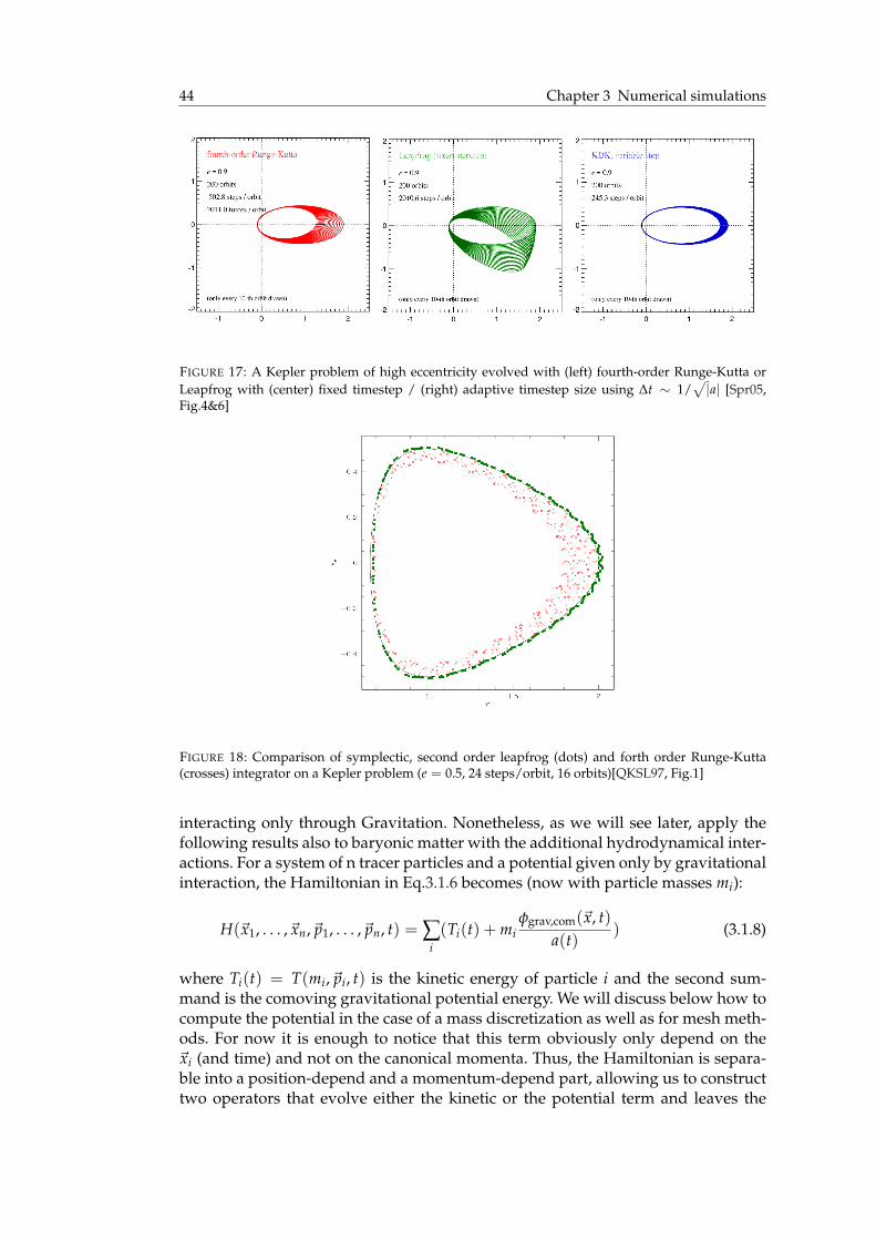
44 Chapter 3 Numerical simulations
FIGURE 17: A Kepler problem of high eccentricity evolved with (left) fourth-order Runge-Kutta orLeapfrog with (center) fixed timestep / (right) adaptive timestep size using ∆t ∼ 1/
√|a| [Spr05,
Fig.4&6]
FIGURE 18: Comparison of symplectic, second order leapfrog (dots) and forth order Runge-Kutta(crosses) integrator on a Kepler problem (e = 0.5, 24 steps/orbit, 16 orbits)[QKSL97, Fig.1]
interacting only through Gravitation. Nonetheless, as we will see later, apply thefollowing results also to baryonic matter with the additional hydrodynamical inter-actions. For a system of n tracer particles and a potential given only by gravitationalinteraction, the Hamiltonian in Eq.3.1.6 becomes (now with particle masses mi):
H(~x1, . . . ,~xn,~p1, . . . ,~pn, t) = ∑i(Ti(t) + mi
φgrav,com(~x, t)a(t)
) (3.1.8)
where Ti(t) = T(mi,~pi, t) is the kinetic energy of particle i and the second sum-mand is the comoving gravitational potential energy. We will discuss below how tocompute the potential in the case of a mass discretization as well as for mesh meth-ods. For now it is enough to notice that this term obviously only depend on the~xi (and time) and not on the canonical momenta. Thus, the Hamiltonian is separa-ble into a position-depend and a momentum-depend part, allowing us to constructtwo operators that evolve either the kinetic or the potential term and leaves the
3.1 Discretization techniques 45
other invariant:29:
D(∆t) := exp(∆t·, HkinPoisson) :
~xi(t) 7→ ~xi(t) + ~pi(t)
mi
∫ t+∆tt
dta(t)2
~pi(t) 7→ ~pi(t)(3.1.9)
K(∆t) := exp(∆t·, HpotPoisson) :
~xi(t) 7→ ~xi(t)~pi(t) 7→ ~pi(t)−mi∇~xi φgrav,com
∫ t+∆tt
dta(t)
(3.1.10)
The first operator is hereby called the drift and the second the kick operator accord-ing to their action. Both are clearly symplectic phase-space transformations. Usingthem, we can build an approximation U(∆t) of the exact time evolution operatorU(∆t) = exp(∆t·, HPoisson), which is by construction also symplectic:
U(∆t) := K(∆t2
)D(∆t)K(∆t2
) (3.1.11)
This is the so-called kick-drift-kick (KDK) leapfrog integrator30.It is only an approxima-tion, because, according to the Baker–Campbell–Hausdorff formula, this simple con-catenation of the kick and drift operators lead to additional commutator terms inthe exponent. Therefore it is only the exact time evolution of the slightly modifiedHamiltonian H which omits the commutator terms and thus the error with respectto the original Hamiltonian is of second order in ∆t (cf. [ST92, Eq.14]) and the re-sulting time evolution is typically close to the original one under H. As we havealready seen in Fig.18, this leads to a conservation (up to some fluctuation) of theenergy in numerical simulations.
In general, the range for the time scales in astrophysical systems is, similar to thespatial case, very large since the dynamical time for gravity scales as the reciprocalroot of the matter density, i.e. ∆t ∼ ρ−
12 (cf. [QKSL97]), while for gas it scales even
like ρ−13 T−
12 . Especially in simulation like the one performed for this thesis which
contains also ”cool” gas, we find very high gas (and DM) densities at the cores ofcertain structures and thus have very short dynamical timescales in these regions.Since it would be quite expensive, i.e. cost much computing time, to use the samesmallest time step size which is needed in the densest region for the whole sim-ulation space, it is important to obtain an integration technique that allows us touse adaptive stepping for each tracer particle. First, we have to notice, that usingdifferent time steps for some particles obviously results in loosing the symplecticproperty since the potential and therefore the whole Hamiltonian is not separablein regard to individual particles. Furthermore do we loose simplecticity by loosingtime reversibility if the time-step criterion involves information from the previoustime step. There are several ways to tackle these two problems in order to get at leasttime integrators that are close to energy conservation and the symplectic propertiesof the one used for a fixed step size. A possible approach is to evolve certain par-
29According to [QKSL97, App.A] is is thereby assumed that no explicit time dependence in the co-moving potential.
30By exchanging the role of the kick and drift operator, we would analogously obtain the drift-kick-drift (DKD) leapfrog integrator.

46 Chapter 3 Numerical simulations
ticles as a group more often than others. Duncan, Levison and Lee, for example,proposed herefore to separate the potential term in a long-range and a short-rangepart H = Hkin + Hsr + Hlr similar to the approach of the P3M method that we willdiscuss later (cf. Sec.3.2.1->Hybrids). This allows to use smaller step sizes on localdynamics while using larger steps for the updates of the whole system and reducesthe computation costs significantely. The corresponding symplectic time propaga-tor is a generalization of the standard leap-frog [DLL98, Eq.16]:
U(∆t) := Klr(∆t2
)[
Ksr(∆t2n
)D(∆tn
)Ksr(∆t2n
)]n
Klr(∆t2
), n ∈N
where the concatenation of short-range KDKs only evolve the local group of par-ticles under Hkin + Hsr and form the drift operator for the long-range, overlyingKDK31. This is popular method in modern cosmological simulation and used e.g.by Springel in his GADGET-2 code [Spr05].
Above we noted that the potential is not separable, but if we assume that the forcesbetween particles in small groups, especially two-particle interaction, is negligiblerelative to the total force. By using a global potential this modified Hamiltonianfinally becomes separable and we can apply the KDK method for each particle andsynchronize the whole system at common time step points. Quinn et al. thereforeintroduced a selection operator that depends only on the position of a particle andthus commutes with the kick operator in each integration step DSKD32, renderingsuch time step reversible.
3.2 Overview: Simulation techniques
The following section shall provide an abstract about used simulation techniquesfor both pure N-body and hydrodynamical simulations. In both cases we are (mainly)focusing on methods based on mass discretization, but will also briefly introduceEulerian methods for the hydrodynamics.For the pure N-body simulations, this overview can hereby be also seen as a histor-ical timeline for the evolution of these techniques, since the the methods beginningat the top with the direct sum down to the hybrid methods become more and moreelaborated and efficient (cf. Fig.19).
3.2.1 CDM N-body simulations
In the cosmological standard model (cf. Section 1.4) nearly all of the matter in theuniverse is assumed to be cold dark matter, which can be described as a collision-
31This can be continued recursively by expanding each time the drift operators in the same mannerfor smaller and smaller subgroups and therefore obtaining a range-dependend hierarchy verysimilar to tree methods.
32This works for both the DKD and the KDK methods

3.2 Overview: Simulation techniques 47
FIGURE 19: Plot of size of high-end N-body simulations against their running date (points) and of thecomputing power following Moore’s law (line) [DBS+08, Fig.7]
less, non-relativistic fluid of particles33, which is governed by the Boltzmann equa-tion
∂ f∂t
+~p
ma2∇ f −m∇Φ∂ f∂~p
= 0 (3.2.1)
where f (~x,~p, t) is the phase-space function such that
ρ(x, t) =∫
f (~x,~p, t)d3 (3.2.2)
Additionally to the Boltzmann equation, the gravitational potential Φ must fulfillthe Poisson equation given in Eq.3.1.5.
The most simple approach is to use the particle-based discretization technique asdescribed before, i.e. by sampling the phase-space density of the dark matter fluidby a finite number of tracer particles of a finite mass mi. The force in Eq.3.1.2 therebyis the gravitational force resulting from the gravitational potential Φ of the systemof N particles, i.e. F = −m∇Φ. There are two different ways to approach the result-ing N-body problem and we will briefly outline both of them:
Direct sum The most obvious solution to determine the potential energy at the po-sition of an arbitrary tracer particle i is to just sum directly the contributionsof all the other particles. The usual Newtonian potential function has a singu-larity when we approach a point mass, i.e. for ~x−~xi → 0, but since the tracers
33not to be confused with tracer particles

48 Chapter 3 Numerical simulations
shall be just representatives of a fluid segment consisting of far smaller parti-cles, we are not expecting such a behavior and want to get a finite potentialinstead. As already mentioned in the discretization section, there exist sev-eral methods to smooth out this unwanted two-body effect and will brieflydiscuss two popular ones. In the first one, a gravitational softening parameterε is introduced, which limits the gravitational force at short distances but issmall enough to have no effect on larger scales. The potential function for thisso-called Plummer method hereby becomes:
ΦPlummer(∆x, ε) = −Ga ∑
j
mj
(|x− xj|2 + ε2)12
(3.2.3)
The second possible choice is a kernel method. A spatially smoothed quantity< Q(x) > at any point ~x is hereby obtained by folding Q(~x) with a normal-ized function called the kernel W34
< Q(~x) >W,h~x:= (Q ∗W)(~x, h(~x, )) =
∫Q(~x′)W(~x−~x′, h~x(·))d~x′ (3.2.4)
h is thereby a parameter (function) called the smoothing length. In the discretelimit case of having particles and by replacing the smoothing length functionby the values at the respective particles.
Φi,Kernel(∆x) = ∑j
W(~xi −~xj, hi, hj)Φj (3.2.5)
where Φj := Φ(mj, ∆x) is the contribution of particle j by using the stan-dard Newtonian gravitational potential and hi, hj are the smoothing lengthsfor particle i and j.As we will see further below, the smoothing length in general varies for differ-ent particles. But conservation of energy and momentum can only be ensuredif forces resulting from pairwise interactions are antisymmetric. Thus the ker-nel has to be symmetric to fulfill this requirement. A simple way to build sucha kernel W using one W(∆~x, h) that depends only on one of the smoothinglength is using the so-called kernel-average [HK89, Eq. 2.15]:
W(∆~x, hi, hj) =12[W(|∆~x|, hi) + W(|∆~x|, hj)
](3.2.6)
Another possible way is to simply use the mean smoothing length instead:
W(∆~x, hi, hj) = W(|∆~x|,hi + hj
2) (3.2.7)
Fig.20 shows the gravitational forces resulting by two methods for a two-bodyproblem. For the kernel method we have thereby chosen a symmetrized andrescaled version of the generalized central B-spline kernel [ML85, Eq.21] andthat is also used the pkdGrav/Gasoline simulation codes for both gravita-
34To be more exact, W is here modeled as a functional depending on both ∆x and the local scalelength function h~x. Hence, it is not a folding in the common sense.

3.2 Overview: Simulation techniques 49
tional and SPH smoothing:
W4(∆~x, h) =Nhν·
1− 6( |∆~x|
h )2 + 6( |∆~x|h )3, 0 ≤ |∆~x|
h < 12
2(1− |∆~x|h )3 , 1
2 ≤|∆~x|
h < 10 , otherwise
(3.2.8)
with N being a normalization factor that depends on the dimensionality ν ofthe used space35. ∆~x is hereby the distance between the two particles and thegravitational softening parameter/lengths are set to ε = (hi + hj)/2 = 0.25with hi = 0.35. It is maybe noteworthy that the used spline kernel is by con-struction in C2, which will be become important later on, when we want tocalculate derivatives of smoothed quantities.
We can notice the different results obtained by the altered potentials. In allcases does the force drop to zero for very small scales, which is in agreementof what we would expect for two fluid segments and while the force in theplummer case approaches the standard 2-body force for ∆x ε, the force re-sulting by using the kernel method with kernel-average and mean-h is alreadyidentical (at least) for all ∆x >= max(hi, hj) 36.
Gra
vita
tiona
l for
ce F
Gra
v [a
.u.]
(comoving) distance ∆x [a.u.]
NEWTONPLUMMER
SPLINE (kernel avg)SPLINE (h avg)
0 0.2 0.4 0.6 0.8 1
FIGURE 20: Gravitational force at 2-body interaction using the standard Newtonian (red),Plummer (green) and Spline kernel potential (blue)
In general, the technique of using a direct summation is considered to be themost accurate one since we introduce no further approximations besides themass discretization and the softening for small-scale interactions, but it is alsoby far the most expensive one. It is obvious, that the computing time of thecalculation of the potential energy and the resulting forces and accelerationsfor every of the N particles in the system scales within O(N2), which renderssimulations of systems with larger amount of particles infeasible. Nonetheless
35For the typical case ν = 3 N = 8π
36This is, of course, only true because the kernel is compact.

50 Chapter 3 Numerical simulations
it will be used when a high accuracy is needed and is also partially used inhybrid techniques as we will see below. While the complexity of this methodcannot be altered, the calculations are fortunately highly parallelizable. Thus,there are hardware solutions to reduce the absolute time costs by using paral-lelization techniques on e.g. cell processors or the graphical processing unitson modern graphic cards and even use special-purpose hardware that hard-codes the algorithms used in the calculations as it has been done with thePlummer method in Gravity Pipe (GRAPE) systems. This results in a reduc-tion of the computing time by a fixed, but still significant factor and helpskeep the direct sum method to be competitive with other methods at least forsystems with particle numbers of up to N ∼ 105, but, as can be seen in Fig.19,is already outdated in its ”pure” form for high-end N-body simulations sincethey are now performed for particle numbers that are several orders of mag-nitude above the feasible limit of this method.
Tree The primary solution to overcome the huge computational costs in the particle-based approach is the hierarchical multipole expansion. It uses the fact that thecontributions of particles that are close to each other are hard to distinguishat larger distances. Thus they can be grouped in a good approximation andtheir single gravitational forces can be replaced by a single multipole force. Asimple way to do this is in an hierarchical way resulting in a tree-like struc-ture, where each leaf contains a single particle or a small group of particlesand the nodes represent the groups, that result by first grouping neighbor-ing leaves and then recursively grouping the thereby obtained nodes. Insteadof this bottom-up approach, it is often easier to start at the upper-most nodecontaining all the particles and then subdividing it into the nodes of the nextlower level. When this is done recursively, we also get this structure, but areable to better control the topology of the resulting tree. Fig.21 illustrates thisalgorithm for a so-called oct-tree, where each node is expanded by breakingup the represented three-dimensional space into its octants of half the sidelength. Therefore each node has eight branches37.
FIGURE 21: 2-D schematic illustration of building up an oct-tree. The path for a certain particle,i.e. the nodes containing it have been thereby highlighted. (based on [SYW01, Fig.1])
Trees as a method of organizing particles have many advantages. They allowus to quickly group neighborhoods by ”walking” the tree for a certain leaf to
37Since the illustration here is a two-dimensional projection, we get a subdivision into only four parts.

3.2 Overview: Simulation techniques 51
find all particles at a certain distance to the starting leaf and reduce the com-plexity of this procedure from (N2), i.e. comparing pairwise each leaf with theone we started with, to (logN) in the worst case (which results from the cost ofwalking the tree from the leaf up to the root38). Barnes and Hut proposed sucha tree walk procedure in their paper about hierarchical force-calculation algo-rithms [BH86]. To keep it brief we will just illustrate the algorithm of the walkfor one particle i in the flowchart in Fig.22. The opening criterion is therebygiven by
lj
D(i, j)< Θ (3.2.9)
where lj is the side length of cell j, D(i, j) the distance between the center-of-mass of particle i and cell j and Θ a fixed accuracy parameter called theopening angle.
j=rootstart
walk step :
walk for particle/leaf i:
particle−particle
yes
nois j leaf ?
expand j
yes
no
yes
j= 1.subnode j last subnode ? walk step
j = next subnode
fulfilled ?
opening crit.
walk step finished
no
interaction with i
particle−cellinteraction with i
FIGURE 22: Flowchart of tree-walk algorithm of Barnes and Hut [BH86] to calculate the gravityinteraction for one chosen particle i
But it also enables us to fasten the search for closest neighbors which we willneed e.g. for smoothing hydrodynamics quantities in the SPH method de-scribed below.
One of the problems that occurs with a tree-based method is the implemen-tation of sensible (quasi-)periodic boundary conditions. These are importantto overcome unwanted effects due to the limited size of the simulated vol-ume. Hernquist, Bouchet and Suto [HBS91, §2] discussed a possible approachby using the Ewald decomposition, i.e. an split of the potential in Fourier space
38Assuming to work on a rather balanced tree

52 Chapter 3 Numerical simulations
into a long-range and a short-range part Φk = Φlrk + Φsr
k where39
Φlrk (k) ∼ Φk exp(−k2x2
s )
Φsr(x) ∼ −1a
G ∑i
mi
xierfc(
xi
2xs)
with xi = min~n(|~x − ~xi − ~nL|),~n ∈ Z3 being the distance between ~x andthe closest image (either original or periodic replica) of particle i. The pre-sented short-range potential thereby approximates the real-space solution ofthe Poisson equation by using only the closest images of particles since typ-ically the spatial scale of the potential/force-split xs is significantly smallerthan the side length L of.the simulation volume and the complementary errorfunction (see Eq.2.1.28) drops fast to zero and thereby surpresses interactionswith other than the closest images. Thus, for the short-range potential (andtherefore for particle-particle interaction), we only have to consider the 26 di-rectly neighboring replicated simulation boxes. Only the long-range potentialhas to deal then with the actual infinite number of such replicas, which arethen handled with cell-particle interactions.
It is finally noteworthy that the time cost to construct a tree are ofO(N log N)(N number of tracer particles) since the height of the tree is typically ofO(log N)and the tagging of each node/cell with its total mass and mass momenta isalso accomplished in O(N log N) by starting at the leaves and propagatingresults up to the root. Thus, the overall cost for searching/grouping is in thesame complexity class and therefore gains an advantage in speed against thedirect sum (O(N2)) by loosing accuracy due to the approximation of long-distance particle-particle interactions with particle-cell interactions.
Particle-Mesh As already shortly outlined at the discretization section, the Particle-Mesh methods are using both mass and space discretization to determine thedynamics. A common way in these methods to do this, is to perform the fol-lowing steps
1. Starting with a simulation space that is already discretized by mass (i.e.we have mass particles) we impose also a mesh on the space and cal-culate the density at the mesh points e.g. by using a kernel-like methodsuch that the particle’s mass is put on the neighboring mesh nodes. Thedensity at the m-th mesh point is thus computed by
ρm =1h3 ∑
imiW(~xi −~xm, h) (3.2.10)
where h is the smoothing length and ~xi and ~xm are the positions of thei-th tracer particle and the m-th mesh point. There are some also popularsmoothing kernels W(·) have the form
W(~xm −~xi, h) =∫
W(~x−~xm, h)S(~x−~xi, h)dx (3.2.11)
W(~x, h) = Θ(|~x| − h/2)Θ(h/2− |~x|) ensures that W has a compact sup-39We use here simplified formulas to keep the discussion as brief as possible. The correct formula for
the decomposed potential (and force) can be found in [HBS91, Eq.2.11]

3.2 Overview: Simulation techniques 53
port and h = nδ (δ mesh spacing) combined with the shape functionS(·, ·) define the different schemes such as the Nearest-Grid-Point (NGP)(n = 1,S(~x, h) = δ(|x|)), Cloud-in-a-Cell (CIC) (n = 2,S(~x, h) = W(~x/h))and Triangular-Shaped-Cloud (TSC) (n = 3,S(~x, h) = 1− |~x/h|) scheme.
2. Now we switch to Fourier space by performing a Fast Fourier transform(FFT) upon the mesh.
3. In Fourier space, we can now more easily solve the Poisson equation, i.e.find the corresponding Green’s function.
4. Back in ”normal” space, we can now use the found Green function tocompute first the potential and then the resulting gravitational forces atthe mesh points by using finite-difference representation of the gradi-ent.(cf. Eq.3.1.1).
5. Finally we can reconstruct the forces at the position of the mass particlesusing the same kernel W(·) as in the first step and update their statebased on the time integrator used in the simulation (cf.Section 3.1)
The great advantage of this method is its speed since the computing costs ofthe FFT only scales with N + Nmesh log(Nmesh) where N is the total number ofparticles and Nmesh the number of mesh points. On the other side, its dynam-ics range is limited by the resolution of the mesh (which in turn is restrictedamong other things by the available memory). To increase the resolution andthereby the dynamical range in the regions of interest, adaptive methods likethe Adaptive Mesh Refinement (AMR) have been invented. The AMR therebyworks on the original low resolution “parent” grid and construct a refinementmesh inside the cells where higher resolution is needed and use the attributes(e.g. the gravitational potential) of the parent grid as boundary conditions forthe refined one. This refinement can be done once and for all at the beginningof the simulation (static) or can be performed for several time steps, whichallows to adapt it to the movement of certain interesting structures in space(dynamic).40
Hybrids There are certain ways to combine the presented methods into some hy-brid forms. They are based on the Ewald decomposition that we have alreadyencountered when we discussed periodic boundary conditions for the treemethod. While the long-range forces can be computed most accurately witha PM method, the short-range interactions will be determined by either usingthe direct sum or a tree method. This results in either the particle− particle−PM (P3M) or the TreePM method. Again, AMR could be imposed on the PMpart to improve the performance. The interested reader may be hereby re-ferred to [Xu95] and [HE88] for more details about these hybrid methods andthe according algorithms.
3.2.2 Hydrodynamical simulations
One important modification of the model with pure (cold) dark matter content isthe addition of baryonic matter to match the amount that has been observed in our
40Much more detailed reviews on AMR (and mesh-based methods in general) can be found e.g. in[PLW] and [EDWF85]

54 Chapter 3 Numerical simulations
”real” universe (i.e. Ωb = 0.0456). It is thereby typically assumed that we can handlethis as an additional ideal fluid that is governed by set of equations for mass andmomentum conservation in an expanding universe as seen in Ch.2.1). Additionally,we have the first law of thermodynamics (i.e. internal energy conservation) and thestate of equation for an ideal adiabatic gas41:
P = (γ− 1)ρu (eq. of state)(∂ρu∂t
)~x
+ ~x∇~x(ρu) = −(ρu + P)(
1a∇~x · a~x + 3
aa
)(1.law of TD)
where u is the specific internal energy and γ the adiabatic index, which has in ourcase the value for a monatomic gas, i.e. γ = 5/3. We also moved the correction termof the Hubble flow to the RHS.
Again, there are two principle ways how this fluid and its properties can be treatednumerically, namely in form of a Lagrangian particle method or an Eulerian grid-based method.
The Eulerian methods incorporate a space discretization and solve the hydrody-namical equations on structured or unstructured grids. Each grid cell i has therebya central value for any hydrodynamic variable. In an similar approach as in the PMmethods, reconstruction schemes are then used to reconstruct the values of the re-spective quantity for each point in space, since these informations have been lostdue to the discretization. They are thereby taking the centered values of the cell,in which the ”point of reconstruction” lies, and, for higher-order schemes, these ofthe neighboring cells into account and further allow so to compute the mean of thequantity as well as the boundary values for each cell. Fig.23 illustrates this for threedifferent reconstruction schemes. Since we are not using any simulation code basedon Eulerian methods, we will skip all the details here and refer the interested readerto publications like [Cen92] for more informations about grid-based hydrodynami-cal cosmological simulations.The main idea behind any Lagrangian method is to follow fixed fluid parcels in-stead of calculating the fluid properties at fixed grid points as done in the Eulerianapproaches. By doing this, the Euler equation can be simplified by using its La-grangian form instead, i.e. expressing the LHS as a total derivative along the flowof parcel i:
d(a~ ix)dt
= −1a∇~xΦi,grav,com −
1aρ∇~xPi (Euler equation - Lagrangian form)
A common popular choice to represent this parcels (and get rid of the implicit mesh)of the baryonic fluid is by using discrete mass elements totally analogue to the par-ticle approach for CDM-like matter and reconstructing the continuous fluid quan-tities by using the kernel smoothing method that we have explained for the di-rect sum, i.e. any continuous hydrodynamic quantity is approximated by a discreteform of Eq.3.2.4, where the measure is replaced by the ratio between mass and thedensity of the particle and a symmetrized kernel (cf. Eq.3.2.6/3.2.7) is used. Hence,
41For a non-adiabatic formulation, we would just have to add a cooling term Λ(u, ρ)

3.2 Overview: Simulation techniques 55
FIGURE 23: Reconstruction schemes of various order for grids (in one dimension): (red) piecewiseconstant, (blue) piecewise linear and (green) piecewise parabolic method [DBS+08, Fig.9]
we obtain as the approximated value of A at particle i:
< Ai >= ∑j
mj
ρjAjW(~xi −~xj, hi, hj) (3.2.12)
This kind of methods are therefore referred to as Smoothed particle hydrodynamics(SPH).
The classic approach is to express field quantities in the Euler equation and the firstlaw of thermodynamics by its smoothed counter-parts and then derive a symmetricformulation of them. There are hereby many symmetric forms for an SPH equation.For example, in the case of the Euler equation this symmetrization can be achievedby finding a symmetric form for the smoothed pressure gradient. That may lead tothe following formulas (expressed for static universe in lagrangian form)42:
dvi
dt= −∑
jmj
(Pj
ρ2j+
Pi
ρ2i
+ Πij
)∇iW(~xi −~xj, hi, hj) (3.2.13)
dvi
dt= −∑
jmj
(2√
PiPj
ρiρj+ Πij
)∇iW(~xi −~xj, hi, hj)
The first form is thereby obtained by using the product rule for derivatives duringthe derivation process, while the second equation is derived by simply using a ge-ometric average of the pressure P. In both equations we also added, for the sake ofcompleteness, the additional term Πi j. We don’t want to go into detail, so we justnote here that it models artificial viscosity which becomes important in case of han-dling local shocks. Analogously the first law of thermodynamics becomes (again
42For a very detailed derivation see e.g. [LL03, Ch.2.2]

56 Chapter 3 Numerical simulations
for static universe in lagrangian form)
dui
dt=
12 ∑
jmj
(Pj
ρ2j+
Pi
ρ2i
+ Πij
)(~vj −~vi)∇iW(~xi −~xj, hi, hj) (3.2.14)
dvi
dt=
12 ∑
jmj
(2√
PiPj
ρiρj+ Πij
)(~vj −~vi)∇iW(~xi −~xj, hi, hj) (3.2.15)
(3.2.16)
For both equations we thereby symmetrized first the divergence of the velocity,which is an exact conversion and then used just the arithmetic and geometric meanof the pressure-density term. Thus, while these equations are still exact in the limitof high particle resolution, they may produce significant errors for the internal/ther-mal energy if significant local pressure variations occur. Additionally, it has beenshown that such methods using energy integration may conserve energy well, butnot the entropy even for adiabatic flows.
While these approaches used the first law of thermodynamics to determine the in-ternal energy by integration, another way to calculate u is based on using a entropicformulation trying to get a better conservation for the entropy of the system. For anadiabatic flow thereby applies
u =A(s)γ− 1
ργ−1 (3.2.17)
where A(s) is an entropic function defined by A(s) = P/ργ. The SPH approxima-tion for A at the particle i thereby evolve as (cf.[Her93, Eq.3.10])
dAi
dt=
12
γ− 1
ργ−1i
N
∑j=1
mjΠij(~vj −~vi)∇iW(~xi −~xj, hi, hj) (3.2.18)
where we included again the artificial viscosity, since shocks can generate entropyand therefore A(s) may vary even in the absence of external heat sources or sinks.By using this method to compute the dynamics of the fluid, the total entropy isconserved better compared to the ”energy” approach, but, on the other hand, thethermal energy of the system may not be well conserved.
As Nelson and Papaloizou have noted in [NP94], one important reason for this non-conservative behavior here is the fact that, if hi depends on interparticle distances(e.g. distance of the k-th nearest neighbor) the computation of the pressure forcesfor a specific particle in the equation of motion can be no longer expressed as a sumof simple pairwise interactions. Another ”popular” source of errors in many imple-mentations results from the lack of taking the implicit ∇h correction terms of thederivatives into account.
Recently, there have been newer SPH formulation that tried to overcome the above

3.2 Overview: Simulation techniques 57
errors. One that we want to outline briefly has been proposed by Springel andHerquist [SH02] and derives the equations of motions directly from a Lagrangianof the discrete system by using the thermal energy in the entropic form as the po-tential, that generates the motions of the SPH particles
L(q, q) =12 ∑
imi x2
i −1
γ− 1 ∑i
mi Aiργ−1i (3.2.19)
where q contains both the particle coordinates ~xi and the variable smoothinglengths hi of the particles in the system. The latter ones are thereby selected suchthat a constant mass is contained in the smoothing volume 4/3πh3
i ρi for all particles i.This results in N constraints for this system. Solving the equations of motion underthese constraints, we get an fully conservative formulation:
d~vi
dt= −∑
jmj
(f j
Pj
ρ2j∇iW(~xi −~xj, hj) + fi
Pi
ρ2i∇iW(~xi −~xj, hi) + ΠijW(~xi −~xj, hi, hj)
)(3.2.20)
where the kernels of the pressure terms are the asymmetric ones depending onlyon the smoothing length of one particle and fi given by
fi = (1 +hi
3ρi
∂ρi
∂hi)−1
contains the correction terms for the variable smoothing length.
At the end of our description of SPH, we finally want to discuss a major advantagethat arises by using a kernel with compact support like the spline kernel and itssymmetrized versions. Independent from the choice of the formalisms the summa-tion for obtaining smoothed quantities has only be performed over the particles ly-ing in the support. Determining hi for example by the k-th nearest neighbor method,all these particle.can be found inside a 2hi-ball centered on the given particle i since,by construction, any hj of a particle in the set of the k-th nearest neighbors cannotbe larger than 2hi. The number of particles in this ball is typically much smallernumber than the total number of tracer particles. A fast way to perform the searchfor these particles in the ball makes again use of trees. In such TreeSPH methods, wethen have an (additional) K-D tree containing only the baryonic matter and whichis typically balanced to minimize the depth and therefore most efficient for thesesearches.
Additional Physics in Baryonic Matter
In contrast to CDM, baryonic matter is involved in various physical processes andinteractions with its environment. A very important one hereby is the ability toform stars, i.e. very dense lumps of baryonic matter heating itself (and the nearbyenvironment) by nuclear fission. In the universe, this star formation and evolutionis a very complex process intensively studied by an own subfield in astrophysics.

58 Chapter 3 Numerical simulations
Cosmological simulation fall short by far of meeting the requirements in dynam-ical range and resolution that would be necessary to even coarsly simulate theseprocesses. For example, in our simulations, single gas particles still have a massof more than 10 million suns and therefore already represent huge clouds formingits own microcosmos that contains multiple parallel process leading to gas form-ing stars and vice-versa. Thus, simulation codes include these processes rather byan analytical approach that uses models describing the ensemble properties of thisprocesses on a scale that can be matched by the resolution of the simulation. Thisis achieved by imposing several criteria on the gas i.e. e.g. a density minimum thathave to be met by our discretized gas particles in order to spawn then new starparticle that represents the net production of stars by this gas cloud matching thestar formation rate predicted by the used model43. This results then in a similiarevolution of baryonic matter bound in star mass as shown in Fig.24 for one of oursimulation runs.
0
0.01
0.02
0.03
0.04
0.05
0 2 4 6 8 10 12 14
ρ / ρ
crit
age of universe [Gyr]
Gal0
GasStars
z=1
FIGURE 24: Evolution of star and gas mass in Gal0
A basic requirement to get dense gas for star formation is having a cooling pro-cess included, that allows gas particles (composed of hydrogen, helium, but alsoof heavier components (metals)) to emit internal energy to the environment (e.g.by collisional excitation/reionization, recombination or Bremsstrahlung). This canbe modeled by an additional cooling term in the first law of thermodynamics pre-sented earlier. In the same way, also external heat sources like supernova, activegalactic nuclei (AGN) and UV Background feedback are added that can reheat thegas and thus prevent star formation. Another effect of supernovae that can be alsotaken into account is the enrichment of the universe with heavier elements, i.e. toincrease its metalicity.43To bound thereby the increase of the number of particles in the simulations, the number of star
particle that each gas particle can spawn is normally restricted to be relatively small.

3.3 Initial conditions 59
3.3 Initial conditions
In chapter 1 we have explained that it is possible to use the CMB ”snapshot” toderive the statistics of the matter distribution on the last scattering surface and dueto our cosmological principles therefore the overall statistical properties of this dis-tribution in the universe at that early time. One important result hereby was σ8,which, as we have seen, characterizes the amplitude of the mass power spectrumthat we will now use, combined with the Zel’dovich approximation, to obtain theinitial conditions for our cosmological simulation at an arbitrary early time after thelast scattering.
Therefore, we simply have to perform the following steps:
1. We have to choose an initial time / redshift / scale factor ai, at which we wantto start our simulation (in our case ai = 0.01882, i.e. z ≈ 52)
2. The particles are then put on a (regular) grid with coordinates ~xj
3. We then obtain a realization of gaussian distribution δ~k (cf. CMB / linear the-ory) on the grid in fourier space that matches the power spectrum defined byσ8 = 0.8:
δ|~k| = N (0, L3boxPlin(|~k|, ai, σ8))
4. Based on the Gaussian compute S(~k) = iδ~k~k|~k|2
for each grid point
5. Now we can displace particles according to the Zel’dovich approximation:
∆~x = D+(ai)S(~x)
6. And analogly, we assign initial velocity with respect to initial density / dis-placement:
~v = D+(ai)S(~x)
3.3.1 Resolution refinement / Zoom technique
Since we are only interested to study the attributes and evolution of just one galac-tic halo in detail, it is not necessary to use the same high resolution for the wholesimulation volume. Instead, we can restrict the highest resolution on the region ofinterest. This is done by first running a low-res simulation to identify an interestinggalaxy. The positions of the particles belonging to its neighborhood then define thehigher-res region at the initial conditions by tracing them back in time. We haveillustrated this in Fig.25 for the Gal0 initial conditions of the common dark mattercontent of both DM and Hydro simulation. In the picture on the top, we can seein blue the low-res grid of the initial simulation run. In green there is then a rect-angular higher-res region. The yellow and red particles mark finally the regions ofhighest resolution. As can be noticed in the sequence of zooms in the bottom row ofFig.25, they are chosen in a way to match the spheres of a certain mean overdensityaround the galaxy, which leads to their irregular shape but allows us once more tokeep the number of particle in the ”uninteresting” parts of the simulation volume

60 Chapter 3 Numerical simulations
as low as possible and use the saved computational power to increase instead thedynamic range in the interesting regions by spending more particles there.
FIGURE 25: Zoom technique based on results of Gal0 : Blue particles with highest mass for lowestresolution (mParticle = 2.377 · 1011 M) and red particles for highest resolution (mParticle = 1.792 ·106 M): (top) slice at IC (below) projection of full box and zooms at final time of simulation
3.3.2 Baryonic matter
For the hydrodynamic simulation we also need to populate our universe with bary-onic matter. Performing the ”zoom” technique that we explained earlier for the darkmatter particles, we can then restrict ourselves to add the additional baryonic mat-ter in the region of highest density. This can be done without causing any majorerrors as hydrodynamics are local and the zoom techniques ensures that the galaxyof interest and its satellite are all embedded in this same region.
3.4 Actual Simulations
In this last section of this chapter, we finally want to present the simulations thatare the basis for all the analysis in this thesis. We start by discussing the simulationcodes that have been used, i.e. pkdGrav for the pure gravitational interaction andGasoline for the additional hydrodynamics of the baryonic matter and outline thenhow the actual simulation have been done and which parameters have been used.

3.4 Actual Simulations 61
3.4.1 Simulation codes
pkdGrav
The pkdGrav code was originally developed by Stadel and Quinn and finally de-signed by Stadel in 2001 (cf. e.g.[ASQ]). It uses a mass discretization approach ofCDM-like matter combined with a tree method to compute the gravity forces. Oneof its main advantage is, that was designed as a very flexible parallel code. Thisflexibility has been achieved by separation the code in four abstract layers (see alsoFig.26)
MA
ST
ER
PS
T l
ayer
MD
L l
ayerwork
Master node
access
distr.
collect results
data
calculation
to worknodes
working nodes
PK
D l
ayer
PS
T l
ayer
global
data,
return
results
access to other n
odes
communication/
assignment
/data
spawns job
access/resultsremote data
startpassi
ng job
FIGURE 26: Design of pkdGrav code: System of process layers
Master layer The Master layer is running the main part of the simulation, i.e. it con-tains the serial code of the main simulation process. The actual parallelizablecalculations like computing the force for all the tracer particles are thereby nothandled directly in this layer but instead in the PST layer.
PST layer The processor set tree layer is the heart-piece of every parallelized calcu-lation. It contains the code that organizes the distribution of each job receivedfrom the Master layer to the working nodes i.e. spawn the appropriate jobs onthe working nodes, pass them the needed data and collect the results. In anidle state all nodes except for main process on the master node are waiting inthis layer for further directions. The main emphasis in the design of this layerwas thereby to keep it free of code that depends on the actual implementationof the parallelization technique by just using an architecture-independent in-terface.
MDL layer The so-called machine-dependent layer now consists of the implementa-tion the used parallelization scheme, i.e. the remote procedure calls, memorysharing and so on. By the separation of the actual implementation in this layer,pkdgrav can be easily ported to work with different kind of architectures. Inour case we are using MPI as the actual communication/parallelization struc-ture of the MDL.
62 Chapter 3 Numerical simulations
PKD layer While the PST and MDL layer just contain the code to organize the”divide-and-conquer‘’ approach of a certain (physical) calculation, all the ac-tual implementation of the physics is separated into the parallel K-D layer.Despite its name, this is mostly serial code to manage local k-d tree for thegravity calculations and is independent of the parallel framework except forsome remote data access using the MDL layer.
As mentioned, pkdgrav incorporates a tree method using a modified version of theK-D tree with hexdecapole moments to represent the mass at each tree node.Thebuild of the tree is hereby performed in both the PST and the PKD layer, but usingdifferent criteria. The domain decomposition on the PST level has a strong emphasison assigning to each working node a part of the simulation space which ensures afair distribution of the work load and minimize communication costs between thenodes44. To accomplish this, the assumed work load is determined for every tracerparticle. This can be done by e.g. estimating the amount of work needed by thelength of the interaction list or by using the knowledge about the cost of calculatingits acceleration in the prior time step. Beginning with the whole simulation volumethe code in the PST layer then divide the remaining space perpendicularly to thelongest axis into two parts that contain the same amount of work (or in case of anodd number of assigned working nodes the same ratio as the best possible split ofthe nodes in groups of nearly same size) and assigning half of the available work-ing nodes to one part and the other nodes to the other part. Doing this recursively,a binary is obtained that contains exactly one working node in each leaf, i.e. at thebottom level.At this point, the PKD layer takes over. It constructs a local gravity tree in eachnode by first cutting off the empty margins and then simply bisecting the longestaxis. The cut-off is used to overcome the problem of getting empty cells while thebisection of the longest axis ensures that the cell’s axis ratio is close to one. Again,this procedure is repeated recursively and is stopped when a cell only contains acertain amount nBucket of particles or less in each cell45. The gravitational accelera-tion for each particle is then computed by a tree-walking procedure similar to theone of Barnes and Hut that we already discussed in the method section. The maindifference is the fact that our leaves are now containing a set of particles instead ofsingle ones (”buckets”). Thus, for pkdGrav the original algorithm has been modi-fied to work with an opening radius ropen instead of working directly with an openingangle. This is defined by rearranging and slightly modifying Eq.3.2.9:
D <lΘ≈ Bmax√
3/21Θ
=: ropen (3.4.1)
where Bmax is the maximum distance from a particle in the cell to the center-of-mass of the cell and as an approximation we assume hereby, that the center-of-masscoincides with the spatial center of the cell. Similarly to Barnes and Huts tree walk,the open radius is then used to determine the particle-cell and particle-particle in-teraction list with the difference that in case of particle-particle interaction, we haveto add not only one but all particles contained in a ”opened” leaf and the sameparticle-particle list is used for all particles of the same bucket. The direct interac-
44This is equal to the concept of data locality, which coincide in this case with the spatial locality andjustifies the use of a spatial split criterion for the tree even at the PST level
45In our case nBucket = 32

3.4 Actual Simulations 63
tions are then computed using a softening with the spline kernel seen in Eq.3.2.8.
As also already mentioned, to model periodicity is not a trivial task for tree codes.PkdGrav incorporates it by including the 26 closest replicas of the simulation boxinto the particle-particle force calculation and then using the hexadecapole momentexpansion of the fundamental cube directly in the Ewald sum to correct the ob-tained forces for infinite periodic replicas as described for the tree methods.
Finally, for time integration pkdGrav incorporates the KDK timestep scheme. Foreach particle the step size has thereby to fulfill the following criterion based on theacceleration.
∆tAccel ≤ ηAccel
√aε
(3.4.2)
where ηAccel is an accuracy parameter. While a global time step is given, the indi-vidual step size for the particles is then achieved by the dividing this base timestep into substeps as we have explained in the Time integration section until eachparticle meets its respective time criterion.
Gasoline
The Gasoline simulation code [WSQ04] is an extension of the pkdGrav code whichwe described in detail right above. Thus, it uses the same efficient parallel N-bodyapproach, but also includes a TreeSPH method to describe the evolution of bary-onic matter in the universe. Gasoline thereby uses a parallel version of the smooth-ing algorithm developed by Stadel that we use in SKID and other density-relatedcalculations (cf. Sect.4.2.1) setting the interaction distance hi to the distance of thefound k-th nearest neighbor for each gas particle i46.Regarding the dynamics of the baryonic matter, Gasoline implements a wide rangeof cases for cooling including adiabatic, isothermal or implicit energy integrationand cooling processes for Hydrogen and Helium has been modeled as well asIonization processes. On the other side, different reheating feedback have been in-cluded. While the pkdGrav code has defined the time step size for updates basedon acceleration, Gasoline uses the following two addtional criteria, the Courant con-dition and expansion cooling rate defining the individual time step for each gas parti-cle:
∆tCourant ≤ ηCouranth
(1 + α)c + βµmax(3.4.3)
∆tExpand ≤ ηExpandu
du/dtif du/dt < 0 (3.4.4)
with h being the smoothing length, α, β, µmax and c coefficients defining the artificialviscosity term introduced in Eq.3.2.13, u the internal/thermal energy and ηCourantand ηExpand again accuracy parameters.
46In our simulations k = 32

64 Chapter 3 Numerical simulations
3.4.2 Runs & Parameters
The data source of this thesis is not only one pair of simulation runs on pkdGravand Gasoline, but in fact three, henceforth called Gal0, Gal1 and Gal3. All of themstart at the same initial redshift of z = 52. The initial conditions are thereby sim-ilar as they are obtained as realisation of the same initial perturbation field usingthe Zel’dovich approximation method which we have explained in the previoussection. The corresponding CDM matter power spectrum is thereby completely de-fined by fixing the amplitude such that σ8 = 0.8, which is in good agreement tothe most recent estimates obtained by observers. We can convince ourselves of thecorrectness of the initial conditions by simply determining the power spectrum ofour initial snapshot. For Gal0 this is shown in Fig.2747
1e-12
1e-11
1e-10
1e-09
1e-08
1e-07
1e-06
1e-05
0.0001
0.1 1 10
P(k
) [a
.u.]
k (h / Mpc)
very low res, mparticle = 2.377 1011 MO•low res, mparticle = 1.100 109 MO•
high res, mparticle = 1.718 107 MO•very high res, mparticle = 1.793 106 MO•
FIGURE 27: Matter power spectrum of initial conditions of Gal0 shown for the different resolutionschosen by using the Zoom technique
In combination with the zoom technique such that half of the about 1.5 million ini-tial dark-matter particles in each simulation are belonging to the second highestand highest density region, we addionally add gas as baryonic matter48, which isthen distributed in the same way as the dark matter before and in an amount thatmatches Ωb ≈ 0.05, giving us the initial condition of the hydrodynamical simula-tion. To finally obtain comparable initial conditions for both hydrodynamical andpure dark matter simulations, we finally convert all the gas particles to dark matter
47The oscillations are thereby caused by the used discrete grid chosen as initial positions for theparticles before the perturbation.
48There are no stars at the initial redshift. They form later during the simulation run based on theimplemented star formation rules

3.4 Actual Simulations 65
particles to obtain the final version of the initial conditions for the pure gravita-tional N-body code. Thus we have six different initial conditions, that are pairwisematching and all ensure to contain a highly resoluted galaxy halo (cf. Fig.25) at finalredshift that we are able to study.
As the simulations are based on the Λ CDM standard model, we also have to choseseveral parameters (besides those used for generating the initial conditions andsome code-related configuration parameters) before being able to actually run thesimulations. These are shown in Tab.3 and are in agreement with the contraints thathave been listed in Tab.1.
Parameter H0ρ−1/2crit,0 G−1/2 ΩΛ Ωm
Value 2.8944 0.732 0.268
TABLE 3: Parameters of simulated universes
Beside this, the simulations included cooling to allow star formation, but no metalcooling. Additionally, supernovae (SN) and UV Background feedbacks are used aswell, while the feedback of AGN has been ignored.
On this way, the simulation data, i.e. 6 sequences of temporal snapshots containingthe phase-space positions and internal state of each particle, has been obtained.Therefore, the next step, i.e. the first genuine one for this thesis, in the followingchapter is to develop the tools that allow us to retrieve the informations we areinterested in.


CHAPTER 4
EVALUATION TOOLS
In this chapter we will finally present the tools we used to analyze the obtained sim-ulation results. We thereby start with describing the methods to identify the maingalaxy halo in the high-resolution area of our simulation and how to determine itsproperties, i.e. its center, virial radius and density profile. Then we will focus on thetools to find and track satellites halos in and around the main halo, briefly presenttwo different approaches to determine some properties of their orbits, which wewill need in our evaluation and finally close this chapter with the presentation ofthe method used for density fitting of the satellites.
4.1 Main Halo
The main or galaxy halo defines the environment that is in the focus of the studies inthis thesis. It contains one galaxy that is orbited by several accreted substructures,the satellites. Each of our three simulated universes contains by construction onesuch structure within the high-resolution area (cf. Ch.3.3). Fig.28 shows the respec-tive area in the DM realization of the Gal0 simulation.
4.1.1 Finding / Tracking
Since the high-resolution region has been chosen in a way to contain the main haloof interest and its surrounding space at z = 0, we didn’t have to explicitly search itas the coordinates were thus known. Nonetheless, it is quite easy to do so in the casethat neither the coordinates of the region is known nor are there graphical tools liketipsy to quickly and easily determine it. Since it contains the smallest DM particlesand hereby also the their highest concentration right in its center, we can simplycenter on this density peak in the simulation volume.
67

68 Chapter 4 Evaluation tools
FIGURE 28: High-resolution region in Dark matter Gal0 simulation at redshift z = 0
The actual center of the main halo is now chosen such that it coincide with itsdensity peak approximated by the center of mass of the most dense region49. Wethereby use a simple FoF finder and choose the linking length such that the sofound groups are inside a isodensity contour of a few times the virial density (cf.Eq.2.1.25). The main halo can then be identified as the largest of these groups (oris the only one). The virial radius is then the (smallest) radius of a sphere aroundthis center such that the mean (over)density inside this sphere matches the valuegiven by Eq.2.1.25 and has been determined by using nested intervals. The track-ing of the main halo is then simply performed by using the same search algorithmconsecutively at the preceding snapshots in a neighborhood of its location foundat the respective preceding step. Since we are proceeding backwards in time andclose encounters with other halos of the same size except in the case of mergers areunlikely, we are thus able to track the same main halo until the first major mergerevent and track then the largest largest halo involved in it for the times before themerge50.
4.1.2 Density fitting
In the former chapter 2.2 we already have presented the different candidates for amodel that we can use to fit the density profile of the halos. In order to study the
49There may be a small difference between the two coordinates due to deformations of the haloe.g.directly after a major merger, but this is neglectable for most of the halo history
50This is sufficient since the evaluation is focused on only one main halo at times after its last majormerger event.

4.1 Main Halo 69
radial matter distribution of the main halo , we have to perform two steps.
• First, we have to calculate the matter density for several radial distances. Thisis done by partitioning the halo in N equally massive shells51 and computingthe average matter density and radial position of the particles within each ofthis shells. The data points thus obtained approximate the density profile, thatwe want to fit. N is thereby chosen small enough that each shell still containsa reasonable number of particles to average out local fluctuations and, at thesame time, large enough to have enough points for the fitting. For the mainhalo, we have chosen N = 50 for the combined density profile of all mattertypes, while N = 20 for each separate type.
• The second step is the actual fitting of the models to the set of data points(xi, yi), i ∈ 1, . . . , N obtained in the previous step. We treat this as a Non-linear Least Squares Problem as described e.g. in [Bjö96, Ch.9.1]. Hence, we wantto find the (global) minimizer of the sum of squares of N residuals in respectto the model parameters αi
F(~x) =n
∑i=0
f 2i (α1, . . . , αm) (4.1.1)
where the residuals fi are defined by
fi(α1, . . . , αm) = yi − ρmodel(α1, . . . , αm, xi) i ∈ 1, . . . , N
with ρmodel being the function of the density profile of the specific model. Tofind a minimum, we need information about the derivatives of this residualfunctions. Therefore the given model has to be a profile that is at least oncecontinuously differentiable and thus the Jacobian
J(α1, . . . , αm)ij =∂ fi(α1, . . . , αm)
∂αj
exists. This requirement is met by all of our models. The necessary conditionfor a (local) minimum is
∇ f (α∗1 , . . . , α∗m) = J(α∗1 , . . . , α∗m)T f (α1, . . . , αm) != 0
with α∗1 , . . . , α∗m being the searched parameters of the fit.
Our actual implementation of this method is based on the nonlinear least-squares solver of the GNU Scientific Library (GSL)[gsl] which uses the Levenberg-Marquardt algorithm [Bjö96, Alg.9.2.1] to numerically solve this minimizationproblem. We thereby use a weighted version based on the variance in theshells of about 5 % of the total average density.
As an example for the fitting results of the larger main halos we show the resultfor Gal0 at redshift z = 0. The grey dots mark the density at the particle posi-tions obtained by smoothing their masses. One can easily identify the radial posi-tion of several satellites inside the main halo. The yellow points mark thereby the
51or to be more exact same number of particles

70 Chapter 4 Evaluation tools
data points of the averaged radial density obtained in the first step. The lower plotthereby shows the relative error while the grey dotted lines mark the 5 % variancedescribed before.
FIGURE 29: Comparison of Halo fits for main halo Gal0 in DM simulation at z = 0
4.2 Satellites
After having introduced the tools to study the main halo, we now want to explainthe tools needed to identify and analyze its substructures, i.e. the satellites.
4.2.1 Finding / Grouping
In order to analyze and track satellites in and around our main halo, we have firstto identify them ,i.e. group the particle that supposedly belong to the same satellite.The decision whether a particle really belongs to a satellite has to be thereby madein physically reasonable manner such that we are not only able to determine theposition and velocity of each satellite halo, but also other physical properties likeits mass.in a reliable way.
The most simple approach is to use a friends-of-friends(FoF) criterion on the particlesto find groups, i.e. put every particle in the same group than a particle in a cer-tain predefined distance ε. Since the particles are just the discretization of the ”massfluid” in the universe, the choice of ε implicitly defines a (global) density level and

4.2 Satellites 71
all particles inside an isodensity52 contour of this level end up in a common group.An obvious problem of such a percolation method is the right choice of the linkinglength, especially if done globally. In that case, any choice of ε in this ”watershedproblem” may produce results where separate groups are be linked together andother groups in low-density regions not be recognized as they lie beneath the ”sur-face”, i.e. density cut-off. Fig.30 illustrate this by performing a grouping on a cho-sen one-dimensional density profile, which is the superposition of separate groupswith Gaussian-shaped53 density profiles within a Gaussian central halo, Halo 0.The falsely recognized groups have been marked in red to point out this describeddeficiency.
0
20
40
60
80
100
0 0.2 0.4 0.6 0.8 1
dens
ity [a
.u.]
x [a.u.]
total densitymain halo
halo 1halo 2halo 3halo 4
0
20
40
60
80
100
0 0.2 0.4 0.6 0.8 1
dens
ity [a
.u.]
x [a.u.]
wrongly groupedwrongly not grouped
correctly groupedtotal density
halosdensity limit
0
20
40
60
80
100
0 0.2 0.4 0.6 0.8 1
dens
ity [a
.u.]
x [a.u.]
wrongly not groupedcorrectly groupedgrouping borders
total densityhalos
FIGURE 30: Illustration of results using various grouping methods on a (left) density profile result-ing from superposition of several halos: (middle) FoF (right) DENMAX/SKID. Wrong groupings, i.e.parts of space linked to wrong group, are marked in red, missing grouping, i.e. parts belonging to agroup but not linked to a group are highlighted in grey and correctly linked parts are green
Furthermore, we can see in this example, that this method provide no physicallyconsistent way to determine the mass or other size-related properties since a globalε not only cut off proportionally more particles from the small groups than fromlarge ones, but also add background particles (caused by overlaps in the densityprofile) to the respective group without any physical justification.
Trying to fix at least some of the deficits without loosing the overall efficiency withrespect to computation time, several adaptions were proposed. So e.g. van Kampen
52It is thereby assumed that all the particles in the simulation have the same mass, which is typicallyfulfilled (at least for CDM) by construction via mass discretization.
53We use the bell-shaped profiles since they share with simulated halo density profiles the propertyof being bounded.

72 Chapter 4 Evaluation tools
presented a version called Adaptive FoF that uses a local linking-length computedwith the smoothed local number density instead of a global one (cf. [van95, Ch.2.2]).While this allows us to deal with the problem of different background densitiesbetter than the original and is nearly as fast as the original algorithm, it still lacks areal physical solution of the grouping problem.
DENMAX/SKID
Another attempt to identify was designed by Gelb and Bertschinger (cf. [GB94,Ch.1.2]) and named DENMAX. It is a grid-based method that tries to find localmaxima in the density field to identify group. It accomplishes its goal by perform-ing the following steps consecutively:
1. The density field is once interpolated onto a regular (rectangular) grid in thesame kernel-based fashion as done for the Step 1 in the PM method describedin Ch.3.2.1, i.e. by using e.g. the CIC or TSC reconstruction schemes.
2. For each particle a ”tracer particle”54 is then placed at the same position as itsoriginal partner.
3. The tracer particles are then moved in small finite steps along the density gra-dient which is obtained by employing an the derivative of the used kernel55
d~xdτ
:= ∇ρ = ∑i
miW(~xi −~xm, h)
The time variable τ is thereby purely fictitious symbolizing the flow of thetracers along the density gradient and has no meaning in a physical sense.Time integration is done here in the most simple way. For each ”time step”each tracer is pushed into the direction of the gradient evaluated at its currentposition by a fixed spatial step size ∆xstep. This ∆xstep here simply determinesthe resolution of the final result, i.e. larger steps tend to force tracer particlesto ”jump over” small local maxima to run into larger ones while smaller stepsallow to find even the smallest perturbations in the density field - usually thegravitational softening length used in the corresponding N-body simulationis hereby considered as a appropriate step size.We also may notice (again) that if the Kernel and therefore its gradient has acompact support56 the same conclusion holds as in Ch.3.2.2 and the sum hasto consider only term from grid nodes in a certain neighborhood around theposition of the tracer particle for which we want to determine the next move.The position updates for each tracer are stopped if they have reached a localmaximum and thus started to oscillate around this attractor, i.e. not leavingan 2∆xstep-ball anymore.
54In the previous chapters, we already used this name for the particles obtained by mass discretiza-tion that are then used to trace the fluid parcel which they represent. In this chapter, we will referto this kind of particles simply as ”particles” and reserve the term ”tracer particles” only for imag-inary mass-less particles used in some grouping algorithms.
55We have put the linking length prefactor in Eq. 3.2.10 into the kernel as well.56which is obviously true for any kernel of the form Eq.3.2.11, but also for the Spline kernel (→ SKID)

4.2 Satellites 73
4. After having concentrated all the tracer particles around the density maxima,they can be easily grouped using e.g. FoF with a linking length of 4∆xstep.After this, the ”origin particles” of the tracers are labeled with the group in-formation and the tracers are deleted.57
5. The final step now brings in the physical aspect we demanded by removingall the particles from each group that are not gravitationally bound to it. Ev-ery group can be then treated separately since the binding energy and thusthe potential energy is determined only with respect to the particles in therespective group according to (using comoving quantities vpec and φcom, cf.Eq.3.1.6)
Eb =12
mi[a|vi,pec − vcm,pec|+ a|~xi −~xcm|
]2 +miφcom(~xi)
a(4.2.1)
with xcm and vcm,pec being the center and the peculiar velocity of the center ofmass of the group corresponding to particle i.
Having calculated the binding energy for each particle in a group and whilestill finding unbound particles (i.e. with binding energies above zero), the par-ticle with the highest value is removed from the group and the computationof the binding energy is performed again for the whole remains of that groupwhile looking again for unbound particles.
A modification of this standard DENMAX is the so-called Spline Kernel InterpolativeDenmax (SKID) algorithm which have been proposed by Stadel et al. [Sta01, Ch.4].Instead of working with a grid to represent the density, it uses a particle-based ap-proach which is very similar to the SPH method seen in Ch.3.2.2. This avoids theresolution problem of the grid-based method. The DENMAX algorithm has to beslightly modified in the first step by calculating the density based on the particlemasses and the Spline kernel (see Eq.3.2.8). The local linking length hi is therebyagain chosen as the distance to the k-th closest neighboring particle and the gradi-ent then reconstructed by using also the spline kernel and sum up the contributionsof these neighboring particles instead of the grid nodes. Supplementary, there canbe included additional steps in both algorithms to improve the results like filteringthe tracer particles before the search step based on a minimum density or, in case ofgas particles, criterion, which would allow to ignore both background and hot gaswhich both usually don’t belong to any satellite. Furthermore, before and after the”unbinding” step, groups that are smaller than a certain threshold Nmembers can bedropped. This helps to ignore fake groups based on numerical artifacts in the back-ground and increase the overall speed since the unbinding process has no longer todeal with them, but also puts a limit onto the size of real groups that can be found(and traced).
The right illustration in Fig.30 now shows the result for the DENMAX/SKID group-ing method for the same density profile that we already used for the FoF. While itnow manages to detect Halo 1-3 correctly, there occurs a problem if halos show asignificant overlap. While in the case of Halo 1 and 3 this results in a rather small
57Hence, if we refer below to a group we mean the group of the ”origin particles”.
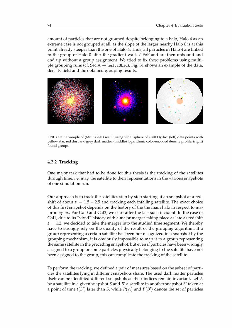
74 Chapter 4 Evaluation tools
amount of particles that are not grouped despite belonging to a halo, Halo 4 as anextreme case is not grouped at all, as the slope of the larger nearby Halo 0 is at thispoint already steeper than the one of Halo 4. Thus, all particles in Halo 4 are linkedto the group of Halo 0 after the gradient walk / FoF and are then unbound andend up without a group assignment. We tried to fix these problems using multi-ple grouping runs (cf. Sec.A→ multiSkid). Fig. 31 shows an example of the data,density field and the obtained grouping results.
FIGURE 31: Example of (Multi)SKID result using virial sphere of Gal0 Hydro: (left) data points withyellow star, red dust and grey dark matter, (middle) logarithmic color-encoded density profile, (right)found groups
4.2.2 Tracking
One major task that had to be done for this thesis is the tracking of the satellitesthrough time, i.e. map the satellite to their representations in the various snapshotsof one simulation run.
Our approach is to track the satellites step by step starting at an snapshot at a red-shift of about z = 1.5− 2.5 and tracking each infalling satellite. The exact choiceof this first snapshot depends on the history of the the main halo in respect to ma-jor mergers. For Gal0 and Gal3, we start after the last such incident. In the case ofGal1, due to its ”vivid” history with a major merger taking place as late as redshiftz = 1.2, we decided to take the merger into the studied time segment. We therebyhave to strongly rely on the quality of the result of the grouping algorithm. If agroup representing a certain satellite has been not recognized in a snapshot by thegrouping mechanism, it is obviously impossible to map it to a group representingthe same satellite in the preceding snapshot, but even if particles have been wronglyassigned to a group or some particles physically belonging to the satellite have notbeen assigned to the group, this can complicate the tracking of the satellite.
To perform the tracking, we defined a pair of measures based on the subset of parti-cles the satellites lying in different snapshots share. The used dark matter particlesitself can be identified different snapshots as their indices remain invariant. Let Abe a satellite in a given snapshot S and B′ a satellite in another.snapshot S′ taken ata point of time t(S′) later than S, while P(A) and P(B′) denote the set of particles

4.2 Satellites 75
assigned to these satellites by the grouping. The first measure is given by
Inv(A, B′) =µ(P(A) ∩ P(B′))
µ(P(A))(4.2.2)
where µ(·) denotes an arbitrary measure (in the mathematical sense) like the num-ber of particles in a given set or its mass. In the case of counting particles, whichwe used in our analysis, Inv(A, B) is thereby the portion of particles in A that alsobelong to B. Similarly, the second measure Corr compares the set of particles incommon to the total set of particles in B
Corr(A, B′) =µ(P(A) ∩ P(B))
µ(B′))(4.2.3)
Hence, Inv(A, ·) contains the information where the particles of A end up in S′ andCorr(·, B′) about the origin of the particles in B′ in S. The two matrices obtained byapplying these measures on all groups in both snapshot is then used to identify therepresentations of the same satellite at the two snapshots and determine their inter-actions like mergers or stripping in the time segment in between. To avoid gettinglost in details, the full description of the algorithm is skipped here. Instead, we onlyoutline the criteria used to identify the representation of one satellite in the consecu-tive snapshot excluding any ”major” interaction like mergers with other satellites orthe main halo. We therefore introduce a new parameter pcrit. It defines the minimalvalue for Corr(A, B′) and Inv(A, B′) to call the relation between A and B to be sig-nificant. For example, in the most simple case of having a satellite, whose represen-tation is group A in S and group A′ in S′, without any (significant) interaction withthe environment, we expect that Corr(A, A′) > pcrit and Inv(A, A′) > pcrit whileCorr(A, B′) < pcrit, Corr(B, A′) < pcrit, Inv(A, B′) < pcrit and Inv(B, A′) < pcrit forall groups B 6= A in S and B′ 6= A′ in S′. The right tuning of pcrit is thereby essen-tial. While large values may cause, that we do not recognize the representation ofthe satellite in S′, e.g. if it has faced strong tidal stripping or a merger in the meantime, a smaller setting may lead to falsely interpret inaccuracies in the groupingsometimes as mergers, at which point the tracking of the satellite as an individualwould be stopped.
As already mentioned, there are a lot of cases beside this simple one to take intoconsideration when comparing the groups of two snapshots including the fact thata satellite may even leave the volume of space that has been grouped to return ata later point in the simulation. The interested reader may be referred to the Ap-pendix B, where we present all these cases and other aspects of the algorithm inmore detail.
4.2.3 ”Twin” Matching
As mentioned in the motivation, our goal is to compare the hydrodynamical andpure DM simulation by studying satellite ”twins”, i.e. satellites formed in both thepure DM and the hydrodynamical simulation from the same perturbations at the
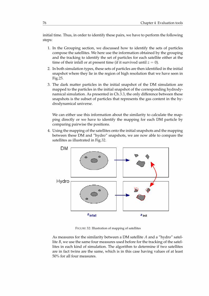
76 Chapter 4 Evaluation tools
initial time. Thus, in order to identify these pairs, we have to perform the followingsteps:
1. In the Grouping section, we discussed how to identify the sets of particlescompose the satellites. We here use the information obtained by the groupingand the tracking to identify the set of particles for each satellite either at thetime of their infall or at present time (if it survived until z = 0).
2. In both simulation types, these sets of particles are then identified in the initialsnapshot where they lie in the region of high resolution that we have seen inFig.25.
3. The dark matter particles in the initial snapshot of the DM simulation aremapped to the particles in the initial snapshot of the corresponding hydrody-namical simulation. As presented in Ch.3.3, the only difference between thesesnapshots is the subset of particles that represents the gas content in the hy-drodynamical universe.
We can either use this information about the similarity to calculate the map-ping directly or we have to identify the mapping for each DM particle bycomparing pairwise the positions.
4. Using the mapping of the satellites onto the initial snapshots and the mappingbetween these DM and ”hydro” snapshots, we are now able to compare thesatellites as illustrated in Fig.32.
FIGURE 32: Illustration of mapping of satellites
As measures for the similarity between a DM satellite A and a ”hydro” satel-lite B, we use the same four measures used before for the tracking of the satel-lites in each kind of simulation. The algorithm to determine if two satellitesare in fact twins are the same, which is in this case having values of at least50% for all four measures.

4.2 Satellites 77
4.2.4 Orbits
As we stated, we are interested in studying the properties of the orbits of the satel-lite, especially for determining the possible danger which the satellites impose onthe inner regions or, to be more exact, a galactic disk. Thus, we are mostly inter-ested in the distance to the central group at the point of closest approach, i.e. thepericentric distance. We followed two possible ways to deal with this goal, onesemi-analytical and one numerical and even if we ended up using the first methodas we abandoned the study of further properties of the orbit besides the peri- andapocentric distance, we will present approaches both for the sake of completenessof presenting the work performed for this thesis.
Effective potential
The ”semi-analytical” way to extrapolate the pericentric distance is to compute thecomoving effective potential defined by
Veff,com(x) = a · L2com
2mx2 −Φgrav(x) (4.2.4)
with Lcom = m(x × x) is the comoving angular momentum. and compare it to thesum of kinetic and potential energy based on the position of the center-of-mass andits drift velocity.of each halo in the rest frame of the center of potential. Fig.33 illus-trates this by plotting the effective potential and the energy for one satellite in a se-lected snapshots. The peri- and apocentric distance thus determined are marked.
-0.007
-0.006
-0.005
-0.004
-0.003
-0.002
-0.001
0
0 0.2 0.4 0.6 0.8 1 1.2 1.4 1.6
spec
ific
Ene
rgy
[a.u
.]
r/Rvir
eff. PotentialEnergy of satellite
PericenterApocenter
FIGURE 33: Determination of pericentric and apocentric distance using effective potential

78 Chapter 4 Evaluation tools
Time integration
The first way is to use the time integration scheme that we presented in Ch.3.1.2, i.ethe symplectic leap-frog algorithm.
Since long-time errors are not such an issue as we will only simulate at most oneorbit, we will approximate the results by taking only the conservative gravitationalpotential based on the density fit of the main halo into account, i.e. we use Eq.3.1.9and 3.1.10 to update the phase-space coordinates for each step for an adaptive timestep size ∆t ∼ 1/a. Influences on the orbit like dynamical friction have thereby notbeen taken into account.One problem hereby is to handle the integral in both operators. For complex scalefunctions a(t), like the one for the ΛCDM model that we are using (cf. Eq.1.4.2), thisintegral can be hardly solved analytically. Thus we have to numerical methods todetermine both the kick and the drift term. We thereby implemented three differentmethods
• The most exact and most expensive method is numerical integration usingRomberg’s method for open intervals as presented e.g. in [GP08, Ch.6.7]. Wethereby use a version with an iterative refinement to obtain an error below agiven threshold.
• The second possible way to tackle this problem is a linear approximation ofa(t). Having a look at the ”velocity” of expansion plotted for the time periodof interest versus the redshift in Fig.34, we can notice that due to rather smalldifference in a(t) over time, a(t) can be approximated for very small timesteps quite well by a linear function with the slope a(t + ∆τ/2), which canthen be integrated quite easily.
0.05
0.055
0.06
0.065
0.07
0.075
0.08
0 1 2 3 4 5 6 7 8
da/d
t [km
s-1
Mpc
-1]
∆t [Gyr]
FIGURE 34: Change of scale parameter da/dt over time

4.2 Satellites 79
The kick and drift operator then become:
D(∆t) :
~xi(t) 7→ ~xi(t)− ~pi(t)
mi a(t+ ∆τ2 )
(a(t + ∆τ)−1 − a(t)−1)
~pi(t) 7→ ~pi(t)(4.2.5)
K(∆t) :
~xi(t) 7→ ~xi(t)
~pi(t) 7→ ~pi(t)−mi∇~xi φgrav,comlog( a(t+∆τ)
a(t) )
a(t+ ∆τ2 )
(4.2.6)
• The last and most simple approach is to assume a static universe for the timeof the orbit. The time integrals therefore sum up to be the time step size ∆τ(or half this value in the case of the kick operator).
The resulting orbits determined using this Leap Frog method is shown in Fig.35.
-0.0014-0.0012
-0.001-0.0008
-0.0006-0.0004
-0.0002 0
0.0002 0.0004-0.001
-0.0005
0
0.0005
0.001
0.0015
0.002
0.0025-0.002-0.0015
-0.001-0.0005
0 0.0005
0.001
orbitapocenterpericenter
comoving x
comoving y
-0.012
-0.011
-0.01
-0.009
-0.008
-0.007
-0.006
-0.005
-0.004
FIGURE 35: Determination of orbit including pericentric and apocentric distance using LeapFrog andcolor-coded potential energy


Part III
Evaluation


CHAPTER 5
EVALUATION/COMPARISON OFGALAXY HALOS
As outlined in the motivation, our goal is to analyze the impact of baryonic matteron the structures of the universe and their evolution. We therefore start to have acloser look at the three galaxy halos that we obtained by the numerical simulationand which will host the satellites we want to study closer in the next chapter.
The first property we determined in the progress of identifying and tracking them istheir (comoving) virial radius. In Fig.36 we plotted the results we obtained therebyfor Gal358.
We can see that the comoving virial radius increase even despite the expansion ofthe universe for both simulation types as the mass grows respectively as shownin Fig.13. But given a certain redshift the curves for the same halo in the DM andHydro simulation start to differ as the radius of the virialized halo in the DM sim-ulation tends to become larger than its Hydro counterpart, even if the differenceis never more than 3% of their absolute values. To illustrate this, Fig.37 shows ascatter plot59. We additionally marked the points that refer to data obtained fromsnapshots before z = 0.8.
58In the following evaluation we will often only embed the plots of the results of only one examplarysimulation run, main halo or satellite into the text while also referring to the results of the rest. Thecorresponding missing plots have been skipped in order to not distract the reader with two manysimilar plots. But the interested reader can find them nonetheless in Ch. C in the Appendix
59The data points have been obtained by linearly interpolating the radii of the Hydro simulations forthe snapshots times of the DM simulation in the case that has been no snapshot been made at thesame time in both simulations.
83

84 Chapter 5 Evaluation/Comparison of Galaxy Halos
170
180
190
200
210
220
230
0 0.5 1 1.5 2
Rvi
r,co
m [k
pc/h
]
Redshift z
Gal3
DMDM
HydroHydro
FIGURE 36: Comparison Evolution of comoving virial radius for Gal3
180
185
190
195
200
205
210
215
220
225
230
185 190 195 200 205 210 215 220 225 230
Rvi
r DM
[kpc
/h]
Rvir Hydro [kpc/h]
Gal0 z<0.8Gal0 z>=0.8
Gal1 z<0.8Gal0 z>=0.8
Gal3 z<0.8Gal3 z>=0.8
FIGURE 37: Comparison Evolution virial radius
An exception are the values for Gal1. By studing the graphs, it can be concluded thatthe main halo took part at a major merger at about z = 1 in both simulation types.Looking at the snapshots shown for the hydrodynamical simulation in Fig.38, thiscan be confirmed.

85
FIGURE 38: Major Merger in Gal1: snapshots with logarithmic density plot (box marks virialized halo)
The difference in the radius can have two reasons.
• The halo in the DM simulation accreted more mass than its hydrodynamicalcounterpart. To check this we plot in Fig.39 the mass inside concentric ballsof different radius around the center of the main halos. It can be seen, thatthe region around the main halo in the pure DM simulation is more massivethan in the hydrodynamical one, which can explain the increased virial ra-dius. This discrepancy can be detected up to the borders of the region of highresolution. To pinpoint the source of this additional mass we now distinguishbetween the different kind of particles in the simulation data, i.e. DM par-ticles of four different masses due to the four different resolutions and thebaryonic particles or, in case of the pure DM simulation, the DM particles thathave been used to substitute the gas in the initial conditions. In Fig.40, wethus plotted the mass of all these different kind of particles inside a sphereof 270 kpc, i.e. approximately the virial radius, over time. While the samenumber and therefore mass of particles of the highest resolution (res.4) can be

86 Chapter 5 Evaluation/Comparison of Galaxy Halos
2e+11
4e+11
6e+11
8e+11
1e+12
1.2e+12
1.4e+12
1.6e+12
1.8e+12
2e+12
2.2e+12
0 0.2 0.4 0.6 0.8 1 1.2 1.4
M(<
r) [M
O•]
redshift z
Gal3
DM rcom=900kpcHydro rcom=900kpc
DM rcom=450kpcHydro rcom=450kpc
DM rcom=90kpcHydro rcom=90kpc
FIGURE 39: Comparison of mass evolution around main halo for Gal3 in DM and Hydro sim-ulation
0
1e+11
2e+11
3e+11
4e+11
5e+11
6e+11
7e+11
8e+11
9e+11
1e+12
0 0.2 0.4 0.6 0.8 1 1.2 1.4
M(<
r com
=27
0kpc
) [M
O•]
redshift z
Gal3
DM res.3Hydro res.3
DM res.4Hydro res.4
DM converted baryonicHydro baryonic
FIGURE 40: Comparison of mass evolution of different particle types inside ball of rcom =270kpc centered on the main halo for Gal3 in DM and Hydro simulation
found, the mass of both the particles of the second highest resolution (res.3)and the (converted) baryonic particles is significantely higher at z = 0, whichclearly causes the difference of mass seen in the Fig.39. The same effect can
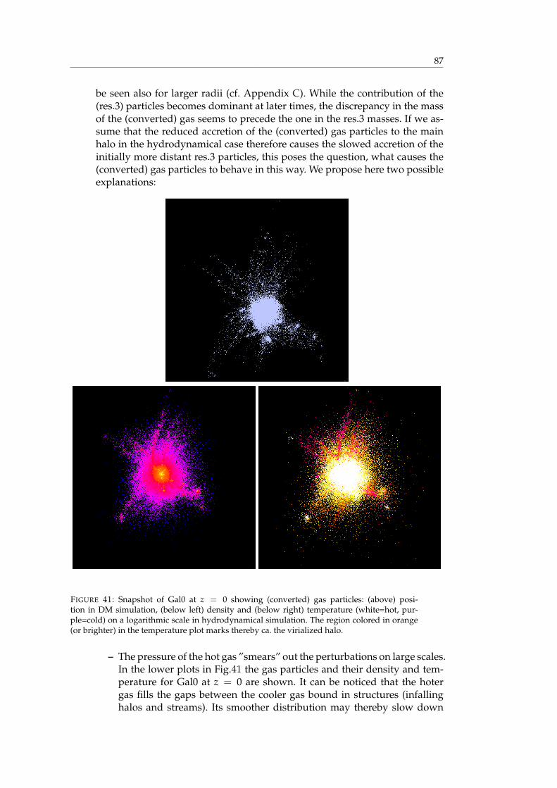
87
be seen also for larger radii (cf. Appendix C). While the contribution of the(res.3) particles becomes dominant at later times, the discrepancy in the massof the (converted) gas seems to precede the one in the res.3 masses. If we as-sume that the reduced accretion of the (converted) gas particles to the mainhalo in the hydrodynamical case therefore causes the slowed accretion of theinitially more distant res.3 particles, this poses the question, what causes the(converted) gas particles to behave in this way. We propose here two possibleexplanations:
FIGURE 41: Snapshot of Gal0 at z = 0 showing (converted) gas particles: (above) posi-tion in DM simulation, (below left) density and (below right) temperature (white=hot, pur-ple=cold) on a logarithmic scale in hydrodynamical simulation. The region colored in orange(or brighter) in the temperature plot marks thereby ca. the virialized halo.
– The pressure of the hot gas ”smears” out the perturbations on large scales.In the lower plots in Fig.41 the gas particles and their density and tem-perature for Gal0 at z = 0 are shown. It can be noticed that the hotergas fills the gaps between the cooler gas bound in structures (infallinghalos and streams). Its smoother distribution may thereby slow down

88 Chapter 5 Evaluation/Comparison of Galaxy Halos
the accretion of the dark matter in the present structures. In contrast, theconverted ”twin” particles in the corresponding DM simulation just addup to the accretion.
– Considering that we initially inserted gas only into the region of highestresolution (cf. 3.3), we certainly face a severe a hydrodynamical bound-ary problem as the pressure in the surrounding lower resolved spacesdrops due to the absence of gas. Comparing the initial comoving vol-ume of the gas and the corresponding converted twin particles with thecomoving volume at z = 0, we obtain, that the gas doubled its volumewhile the converted particles, which are only governed by the total mat-ter density field without such harsh boundary effect between the regionsof highest and lower resolution, are confined to a region of only halfthe initial volume size resulting (at least partly) in the difference seen inFig.40.
The second explanation (and therefore a design flaw in the initial conditions)seems to be more likely the main cause of the difference, but without compa-rable hydrodynamical simulations that are totally filled with baryonic matter,it is hard to quantify the exact contribution of the discussed points.
• Despite the increased total mass of the pure dm main halo, we also notice,that the mass of the ”hydro” halo inside a 90 kpc (∼ 1/3Rvir ball exceeds themass of its dm twin in the same region. Thus, the halos has a different den-sity profiles in the two simulation types. This can also influence the size ofthe virialized halo since it is determined by the mean density inside and amore concentrated mass in the center may lead to a smaller virial radius.Tostudy this closer, we have a look at the results of the density profile fits ofour simulations shown for Gal0 in Fig.42 including the quality determinedby a (weighted) χ2 test. In the results for the simple NFW, we see, that thescale parameter Rs is smaller in the hydrodynamical simulations than in thepure DM ones. Hence, the ”hydro” main halos seem to be steeper in the innerregions. This is expected a percentage of the baryonic matter in the hydrody-namical simulation may cool down and sink deeper into the potential well.The GNFW fit additionally reveals that the logarithmic slope in the hydrody-namical case is slightly above 2 up to half the virial radius Rs ≈ 100kpc/h,which corresponds to the predictions of the isothermal model. On the otherhand, the logarithmic slope of the DM halos determined by the GNFW fitmatches the one predicted by the simplier NFW model as the inner slope isnearly 1 and the scale factor is therefore also the same as in the result of theNFW. The PoLLS fit finally is the most accurate of the three. While the innerregions are quite well fitted by the previous two models, the PoLLS seem tofit the outer regions of the halo better as they seem to become steeper than thelogarithmic slope of 3 modeled by the NFW and GNFW.
In the evolution of the fits, it is difficult to determine any significant change inthe shape of the profile over time. Nonetheless, we want to study the profileof the hydrodynamical halo in Gal0 in Fig.43 more closely. To make the profileat different redshifts comparable, we normalize them by the virial radius andthe halo mass.
It can be noticed, that while the total density profile for radii larger than one

89
1000
10000
100000
1e+06
ρ 0 [I
.U.]
Gal0
DMHydro
1
10
100
Rs
[kpc
/h]
DMHydro
1000
10000
100000
0 0.2 0.4 0.6 0.8 1 1.2 1.4
χ2 /dof
redshift z
DMHydro
1 10
100 1000
10000 100000 1e+06
ρ 0 [I
.U.]
Gal0
DMHydro
1
10
100
1000
Rs
[kpc
/h]
DMHydro
0.01
0.1
1
10
γ
DMHydro
1000
10000
100000
0 0.2 0.4 0.6 0.8 1 1.2 1.4
χ2 /dof
redshift z
DMHydro
1e-05
0.0001
0.001
ρ 0 [I
.U.]
Gal0
DMHydro
10000
100000
1e+06
0 0.2 0.4 0.6 0.8 1 1.2 1.4
χ2 /dof
redshift z
DMHydro
0.01
0.1
1
γ
Gal0
DMHydro
0.001
0.01
0.1
1
10
100
R-2
[kpc
/h]
DMHydro
100 1000
10000 100000 1e+06 1e+07 1e+08 1e+09 1e+10
ρ -2
[I.U
.]
DMHydro
100
1000
10000
100000
0 0.2 0.4 0.6 0.8 1 1.2 1.4
χ2 /dof
redshift z
DMHydro
FIGURE 42: Evolution of fitting parameter of all 4 models for Gal0
1000
10000
100000
1e+06
1e+07
1e+08
1e+09
1e+10
1e+11
1e+12
0.01 0.1 1
ρ(r)
/ M
Hal
o [I.
U.]
r / Rvir
Gal0
total z=0Gas z=0
Stars z=0total z=1Gas z=1
Stars z=1
FIGURE 43: Density profiles of gas, star and total matter in Gal0 at redshifts z = 0 and z = 1
tenth of the virial radius indeed does not change significantly, the slope in theinner region becomes more steeper over time in the same way the gas and starprofile do. A possible explanation can be deduced from Fig.24, wherein weobserve that in Gal0 more than one third of the stars are formed after z = 1.The stars sinking deeper into the potential well and thereby steepening thedensity profile over time. Additionally, a progressive cooling down of the gasand the resulting adiabatic contraction (cf. e.g. [GKKN04]) in the inner region

90 Chapter 5 Evaluation/Comparison of Galaxy Halos
over time could contribute to this developement, but we have not obtaineddata about the temperature field that verifies such an ongoing cooling process.
To summerize the results of this chapter, we can state, that we noticed two differ-ences between the pure DM and the hydrodynamical simulations. The saw that themain halo accretes less mass in the presence of baryonic matter, while it steepensat the same time. The first fact leads and second at least may lead to the result ofa smaller virialized region in the hydrodynamical simulation that has been seenin Fig.36.As we have argued, the increased mass can be caused by a flaw in thechoice of the initial conditions of our simulation, thus we have to remind this possi-bly ”man-made”discrepancy, when studying the masses of the satellites in the nextchapter.

CHAPTER 6
EVALUATION/COMPARISON OFSATELLITES
Our main focus in this thesis lies, as outlined in the preamble, on the studies ofthe accreted substructures of the main halos that we have analyzed in the previouschapter. Our first step is to confirm the difference in the (cumulative) density profilethat has been observed by Macciò before. Fig.44 shows the combined cumulativeprofile for all three halos60, while Fig.45 contains a plot showing the logarithmicnumber density profile for simulation Gal0 which has been normalized by the meannumber density in the corresponding main halo.
0
0.2
0.4
0.6
0.8
1
0 0.2 0.4 0.6 0.8 1
N(<
r)/N
tot
r/rvir
cumulative radial profile of substructures
DMHydro
DMHydro
DMHydro
FIGURE 44: Number density profile of satellites (combined results for Gal0,Gal1,Gal3)
60In this section we often show only the plots of the results of all three main halos combined. Theplots for each halo/simulation run can be looked up in many cases in the Appendix C.
91

92 Chapter 6 Evaluation/Comparison of Satellites
-1
-0.5
0
0.5
1
1.5
2
2.5
0 50 100 150 200 250 300
log
N(R
)/n v
ir
r [kpc]
radial number density profile of substructures
DMHydro
FIGURE 45: Normalized number density profile of satellites (Gal0)
It can be seen that for the hydrodynamical simulations, more satellites are founddeeper in the main halos than in the pure DM run. At the same time there are fewersatellites found in the outer regions of the main halo. If we only regard satellites thatare more massive than 2× 10⁸M (Fig.44), this effect becomes even more distinct.
0
0.2
0.4
0.6
0.8
1
0 0.2 0.4 0.6 0.8 1
N(<
r)/N
tot
r/rvir
cumulative radial profile of substructures
DM, Msat,0 > 2e8Hydro, Msat,0 > 2e8
DM, Msat,0 > 2e8Hydro, Msat,0 > 2e8
DM, Msat,0 > 2e8Hydro, Msat,0 > 2e8
FIGURE 46: Cumulative Number Density profile of satellites heavier than 2× 10⁸ M (combined re-sults for Gal0,Gal1,Gal3)
We have to note that we have found for at least one of the three different initial con-

6.1 Comparison of radial positions/orbits 93
dition more satellites in the hydrodynamical snapshots than in those of the pure DMsimulation. Thus, a possible reason for this difference in the distribution may be,that the partners of the innermost ”hydro” satellites have already been disrupted.Another reason may be, that the distribution of the satellite in both simulation typesis just different due to the influence of the baryonic matter. In both cases we shouldbe able to observe these processes by studying the identified pairs of satellite ’twins’(cf. Ch.4.2.3) at z = 0. We start thereby with comparing their radial distribution inorder to determine if their distribution is in fact different and then focus on theirmass and mass loss to answer the question about a possibly different rate of de-struction.
6.1 Comparison of radial positions/orbits
As described in Section 4.2.3, we identified similar satellites in both simulationtypes using the composition of the satellite at both infall time and at redshift z = 0.As we lost the track for some satellites, the number of satellite twins at present red-shift using both methods exceeds the number of twins we identified at infall timeand successfully tracked until z = 0. 61. For example, in case of Gal1, we identi-fied the highest number of satellites at z = 0, i.e. 181 in the pure DM simulationand 159 in the hydrosimulation lying inside a sphere with a radius of 1.8 times thecorresponding virial radius. The number of identified twins at this redshift is 69.This may be caused by the fact that the partners of unmatched satellites are eitheralready destroyed or just too small or too different from their counterparts to beidentified by the grouping and matching tools.
Despite this rather small number of samples, we want to see if the difference be-tween the (cumulative) number density profiles for this subset of satellites is stillexistent. As seen in Fig.47, this is still the fact.
So, this confirms that we have indeed a difference in the radial position of twinscausing at least some of the observed difference.
Radial Position
Using the found pairs of twins, we now compare the radial position of the satellitespairwise in the pure DM simulation with their hydrodynamical counterparts asshown in Fig.48
It can be noticed that, up to a distance of 0.5 rvir for Gal1 and in an even larger innerregion for the other two simulations, there are, as expected, more data points abovethe line of equal distance. But this plot also shows that there are satellites in theDM simulations close to the center that have hydrodynamical counterparts furtheraway. To bring this out, we plot in Fig.49 the ratio of the radial distances of thesetwins in respect of their distance in each simulation type.
61Thus, the number of data points in following plots including properties at infall and z = 0 is lessthan the number in plot only referring to properties at z = 0. The same is true in respect to thenumber of twins at infall.

94 Chapter 6 Evaluation/Comparison of Satellites
0
0.2
0.4
0.6
0.8
1
0 0.2 0.4 0.6 0.8 1
N(<
r)/N
tot
r/rvir
cumulative radial profile of substructures (twins)
DMHydro
DMHydro
DMHydro
FIGURE 47: Cumulative Number Density profile of satellites (combined results for Gal0,Gal1,Gal3,twins only)
0
0.5
1
1.5
2
0 0.5 1 1.5 2
r z=
0/r v
ir dm
rz=0/rvir hydro
radial position in dm vs. radial position in hydro (all)
Gal0 zfirst <= 0.8Gal0 zfirst > 0.8
Gal1 zfirst <= 0.8Gal1 zfirst > 0.8
Gal3 zfirst <= 0.8Gal3 zfirst > 0.8
FIGURE 48: Comparison of radial positions of satellite ”twins” at redshift z = 0
For the satellites in the hydrodynamical simulation (i.e. upper plot) we can identifyfour regions. In the innermost region up to about 0.7 rvir the satellites are closer to

6.1 Comparison of radial positions/orbits 95
-1
-0.5
0
0.5
1
1.5
2
2.5
0 0.5 1 1.5 2
log(
r z=
0,dm
/rz=
0,hy
dro*
r vir,
hydr
o/r v
ir,dm
)
rz=0/rvir hydro
difference in radial position vs. radial position in hydro (all)
Gal0 zfirst <= 0.8Gal0 zfirst > 0.8
Gal1 zfirst <= 0.8Gal1 zfirst > 0.8
Gal3 zfirst <= 0.8Gal3 zfirst > 0.8
-1
-0.5
0
0.5
1
1.5
2
2.5
0 0.5 1 1.5 2
log(
r z=
0,dm
/rz=
0,hy
dro*
r vir,
hydr
o/r v
ir,dm
)
rz=0/rvir dm
difference in radial position vs. radial position in dm (all)
Gal0 zfirst <= 0.8Gal0 zfirst > 0.8
Gal1 zfirst <= 0.8Gal1 zfirst > 0.8
Gal3 zfirst <= 0.8Gal3 zfirst > 0.8
FIGURE 49: Comparison of radial positions of satellite ”twins” at redshift z = 0
the center than their corresponding counterparts in the pure DM simulations. Inthe second region around 0.8, we find in contrast to the first region many satellitesthat are closer in the DM simulation. At the boundary of the virial halo, we againobserve, that most of the ”hydro” satellites are closer, while in the remaining outerregion, the DM satellites are either at an equal distance than their counterparts (e.g.Gal1) or slightly closer again (Gal3).In the lower plot it is harder to distinguish such regions, but i can be noticed that

96 Chapter 6 Evaluation/Comparison of Satellites
a majority of DM satellites in the innermost region are closer and in the outermostregion farer away than their twins even if this is not so distinct than in the upperplot.
Average distance
The radial positions we analyzed are those of a single time snapshot, i.e. their valuesat z = 0. Thus we expect the radial difference observed in both plots for the inner-most and outermost satellites as they are most likely at their pericenter or apocenterwhile their twins may be at another point in their orbit. A way to get rid of this, wenow focus on orbital elements instead. We therefore determine the length of the pe-riapsis rperi and the apoapsis rapo using the tool described in Section 4.2.4 and defineas the average distance the length of the major-semi axis62 given by (rperi + rapo)/2.Using this average distance instead of the actual radial distance at z = 0, we obtainthe plots in Fig.50 and Fig.51
0
0.5
1
1.5
2
2.5
0 0.5 1 1.5 2 2.5
r z=
0,av
g/r v
ir dm
rz=0,avg/rvir hydro
average distance in dm vs. average distance in hydro (all)
Gal0 zfirst <= 0.8Gal0 zfirst > 0.8
Gal1 zfirst <= 0.8Gal1 zfirst > 0.8
Gal3 zfirst <= 0.8Gal3 zfirst > 0.8
FIGURE 50: Comparison of average distance (length of (pseudo-)major-semi axis) of satellite ”twins”at redshift z = 0
We are now able to distinguish the same two inner regions in the upper plot ofFig.51 that we found in Fig.49. In contrast, the peak in the third region vanished.We furthermore now observe that the outermost satellites in both simulation typeshave twins such that the satellites in the pure DM simulation have smaller average
62Since the orbits are not Kepler orbits as we have a spatially extended halo, the orbits are actuallynot totally elliptical, but at least similar. We thus use henceforth the same terminology, when de-scribing properties of the orbit.

6.1 Comparison of radial positions/orbits 97
-1
-0.5
0
0.5
1
1.5
0 0.5 1 1.5 2 2.5
log(
r z=
0,dm
,avg
/rz=
0,hy
dro,
avg*
r vir,
hydr
o/r v
ir,dm
)
rz=0,avg/rvir hydro
difference in average distance vs. average distance in hydro (all)
Gal0 zfirst <= 0.8Gal0 zfirst > 0.8
Gal1 zfirst <= 0.8Gal1 zfirst > 0.8
Gal3 zfirst <= 0.8Gal3 zfirst > 0.8
-1
-0.5
0
0.5
1
1.5
0 0.2 0.4 0.6 0.8 1 1.2 1.4 1.6 1.8 2
log(
r z=
0,dm
,avg
/rz=
0,hy
dro,
avg*
r vir,
hydr
o/r v
ir,dm
)
rz=0,avg/rvir dm
difference in average distance vs. average distance in dm (all)
Gal0 zfirst <= 0.8Gal0 zfirst > 0.8
Gal1 zfirst <= 0.8Gal1 zfirst > 0.8
Gal3 zfirst <= 0.8Gal3 zfirst > 0.8
FIGURE 51: Comparison of average distance (length of (pseudo-)major-semi axis) of satellite ”twins”at redshift z = 0
distances than their counterparts.
This raise the question whether these lower and higher average distances resultsfrom a different pericenter distance or apocenter distance or both. Thus, we willhave to compare the twin with respect to both distances in the same way, while

98 Chapter 6 Evaluation/Comparison of Satellites
marking the data points of the inner region with ravg,hydro ≤ 0.8rvir,hydro as definedabove in a different way than the more distant twins.
Pericenter distance
The plots in Fig.52 and Fig.53 show that the satellites with larger pericenter distancehave a smaller pericenter distance in the pure DM simulation than in the hydrody-namical simulation.
0
0.2
0.4
0.6
0.8
1
1.2
1.4
0 0.2 0.4 0.6 0.8 1 1.2 1.4
r z=
0,pe
ri/r v
ir dm
rz=0,peri/rvir hydro
pericenter distance in dm vs. pericenter distance in hydro (all)
Gal0 ravg,hydro <= 0.8Gal0 ravg,hydro > 0.8
Gal1 ravg,hydro <= 0.8Gal1 ravg,hydro > 0.8
Gal3 ravg,hydro <= 0.8Gal3 ravg,hydro > 0.8
FIGURE 52: Comparison of pericenter distance of satellite ”twins” at redshift z = 0
The same is true for nearly all satellites with an average distance larger than 0.8rvir,hydro, which may therefore explain the smaller average distance that we observedfor the satellites in the outer regions. In contrast, we do not observe any significanttendency for satellites with lower pericenter distances or lower average distance.

6.1 Comparison of radial positions/orbits 99
-2.5
-2
-1.5
-1
-0.5
0
0.5
1
0 0.2 0.4 0.6 0.8 1 1.2 1.4 1.6
log(
r z=
0,dm
,per
i/rz=
0,hy
dro,
peri*
r vir,
hydr
o/r v
ir,dm
)
rz=0,peri/rvir hydro
difference in pericenter distance vs. pericenter distance in hydro (all)
Gal0 ravg,hydro <= 0.8Gal0 ravg,hydro > 0.8
Gal1 ravg,hydro <= 0.8Gal1 ravg,hydro > 0.8
Gal3 ravg,hydro <= 0.8Gal3 ravg,hydro > 0.8
-2.5
-2
-1.5
-1
-0.5
0
0.5
1
0 0.2 0.4 0.6 0.8 1 1.2
log(
r z=
0,dm
,per
i/rz=
0,hy
dro,
peri*
r vir,
hydr
o/r v
ir,dm
)
rz=0, peri/rvir dm
difference in pericenter distance vs. pericenter distance in dm (all)
Gal0 ravg,hydro <= 0.8Gal0 ravg,hydro > 0.8
Gal1 ravg,hydro <= 0.8Gal1 ravg,hydro > 0.8
Gal3 ravg,hydro <= 0.8Gal3 ravg,hydro > 0.8
FIGURE 53: Comparison of pericenter distance of satellite ”twins” at redshift z = 0
Apocenter distance
For the satellites with larger apocenter and average distance we notice the samerelation between the twins as for the pericenter distance, i.e. smaller values for theDM satellites compared to their twins in the hydrodynamical simulation. But, atthe same time, a significant number of ”hydro” satellites in the upper plot in Fig.55with a small apocenter distance have twins with larger apocenter distances. Thus,

100 Chapter 6 Evaluation/Comparison of Satellites
0
0.5
1
1.5
2
2.5
3
3.5
4
0 0.5 1 1.5 2 2.5 3 3.5 4
r z=
0,ap
o/r v
ir dm
rz=0,apo/rvir hydro
apocenter distance in dm vs. apocenter distance in hydro (all)
Gal0 ravg,hydro <= 0.8Gal0 ravg,hydro > 0.8
Gal1 ravg,hydro <= 0.8Gal1 ravg,hydro > 0.8
Gal3 ravg,hydro <= 0.8Gal3 ravg,hydro > 0.8
FIGURE 54: Comparison of apocenter distance of satellite ”twins” at redshift z = 0
the smaller average distance for the subset of satellites with ravg,hydro ≤ 0.8rvir,hydroseems to mainly result from this reduced apocenter distance.
Influence of infall time
After having pinpointed the source of the closer ”hydro” satellites, we still have tofind the (physical) explanation for it. Comparing the times of first observation, i.e.the time of the first snapshot they were found, in Fig.56, we not only notice that thesatellites in the DM enter at an earlier point than their ”hydro” counterpart, but wealso see that most of the twins with the larger average distance are in fact just attheir first approach into the virialized halo.
At this point the total energy and therefore the apocenter distance decreases fastover time, such that the difference in the DM and hydrodynamical simulations forthe more distant satellites can be at least partly explained by the difference in thetime of approach.
Influence of baryonic matter
One major effect caused by the baryonic matter as already been shown in the lastchapter, when we analyzed the density profile of the main halo. The density pro-file and therefore the potential in the hydrodynamical simulation is steeper in theinnermost parts than their counterparts in the pure DM simulation providing thusa different environment for the satellites in each simulation type. Based on this,we expect that the dynamical friction, which depend on the local density of thebackground, is stronger in the inner parts, which may explain the smaller average

6.1 Comparison of radial positions/orbits 101
-1
-0.5
0
0.5
1
1.5
0 0.5 1 1.5 2 2.5 3 3.5 4
log(
r z=
0,dm
,apo
/rz=
0,hy
dro,
apo*
r vir,
hydr
o/r v
ir,dm
)
rz=0,apo/rvir hydro
difference in apocenter distance vs. apocenter distance in hydro (all)
Gal0 ravg,hydro <= 0.8Gal0 ravg,hydro > 0.8
Gal1 ravg,hydro <= 0.8Gal1 ravg,hydro > 0.8
Gal3 ravg,hydro <= 0.8Gal3 ravg,hydro > 0.8
-1
-0.5
0
0.5
1
1.5
0 0.5 1 1.5 2 2.5 3
log(
r z=
0,dm
,apo
/rz=
0,hy
dro,
apo*
r vir,
hydr
o/r v
ir,dm
)
rz=0,apo/rvir dm
difference in apocenter distance vs. apocenter distance in dm (all)
Gal0 ravg,hydro <= 0.8Gal0 ravg,hydro > 0.8
Gal1 ravg,hydro <= 0.8Gal1 ravg,hydro > 0.8
Gal3 ravg,hydro <= 0.8Gal3 ravg,hydro > 0.8
FIGURE 55: Comparison of apocenter distance of satellite ”twins” at redshift z = 0
distance for the innermost ”hydro” satellites, while the lower density in the outerregion would have an opposite effect on the ratio between the average distance ofthe twins causing the higher average distance in the hydrodynamical case.
The question is now, whether the baryonic content of the satellites have an de-tectable correlation with the radial distribution. To answer this question, we plot

102 Chapter 6 Evaluation/Comparison of Satellites
0
1
2
3
4
5
6
7
8
9
10
0 1 2 3 4 5 6 7 8 9 10
t 0 -
t [G
yr] d
m
t0 - t [Gyr] hydro
time of first observation in dm vs. time of first observation in hydro (all)
Gal0 ravg,sph <= 0.8Gal0 ravg,sph > 0.8
Gal1 ravg,sph <= 0.8Gal1 ravg,sph > 0.8
Gal3 ravg,sph <= 0.8Gal3 ravg,sph > 0.8
FIGURE 56: Comparison of time of first observation
the data already shown in Fig. 50 including the information about the baryoniccontent relative to the total mass in the hydrodynamical simulation at the time ofinfall.
It seems that there may exist a correlation between the percentage of the baryonicinfall mass with respect to the total infall mass and the average distance. We thuswant to have a closer look at this. By plotting the data for the average distanceand the ratio in the average distances of the twins separately, we obtain the resultsshown in Fig.58. The lower plot seems to show no significant relation between theratio of the baryonic matter in the satellite and the difference in the average distanceof the twins. Only a few very baryon-rich satellites show a smaller average distanceto the center of the halo than their twins in the pure DM simulation. By compar-ing this plot with the upper plot and Fig.57, these can be identified as some of theinnermost satellites. The upper plot thereby shows clearly that twins with a higherrelative baryonic content at the moment of infall can be found deeper in the halo.We will discuss a possible explanation for this effect when evaluating the baryonicinfluence on the mass.

6.1 Comparison of radial positions/orbits 103
difference in average distance vs. average distance in dm (all)
Gal0Gal1Gal3
0 0.5 1 1.5 2rz=0,avg/rvir hydro
-1
-0.5
0
0.5
1
1.5
log(
r z=
0,dm
,avg
/rz=
0,hy
dro,
avg*
r vir,
hydr
o/r v
ir,dm
)
-9
-8
-7
-6
-5
-4
-3
-2
-1
0
log(
Mba
ryon
ic,in
fall/
Min
fall)
hyd
ro
FIGURE 57: Comparison of average distance (length of (pseudo-)major-semi axis) of satellite ”twins”at redshift z = 0

104 Chapter 6 Evaluation/Comparison of Satellites
0
0.05
0.1
0.15
0.2
0.25
0 0.2 0.4 0.6 0.8 1 0
0.005
0.01
0.015
0.02
0.025
0.03
Mba
ryon
ic,in
fall/
Min
fall
hydr
o
Mst
ar,in
fall/
Min
fall
hydr
o
rz=0,avg/rvir hydro
total baryonicstar
fit baryonic
0
0.05
0.1
0.15
0.2
0.25
-0.6 -0.4 -0.2 0 0.2 0.4 0.6 0.8 1 1.2 1.4 0
0.005
0.01
0.015
0.02
0.025
0.03
Mba
ryon
ic,in
fall/
Min
fall
hydr
o
Mst
ar,in
fall/
Min
fall
hydr
o
log(rz=0,avg/rvir dm)/(rz=0,avg/rvir hydro)
total baryonicstar
FIGURE 58: Plot of relative baryonic infall mass vs. (above) average distance of hydro satellite and(below) difference in average distance at redshift z = 0

6.2 Comparison of Mass & Mass Loss 105
Interim conclusion (radial distribution)
Started with the goal to relate the higher number density of satellites in the in-ner regions of the main halo to a difference in the radial distribution of the samesatellites, we found, that the innermost ”hydro” satellites have a smaller averagedistance than their twins and are thus more likely found closer to the center. Thisdifference in the average distance results thereby mainly by a reduced apocentricdistance in the hydrodynamical simulation, which may be caused by a stronger dy-namical friction in these inner regions due to a denser central region.
While having provided a first possible explanation, we will now focus on the massthe satellite and its evolution over time for two reasons. On the one hand, as men-tioned in the introduction of this chapter, we are interested to see, if we find cluesfor a higher stability or rate of disruption of satellites in one simulation type. Onthe other hand can a larger (retained) mass of the satellite may cause a strongerdynamical friction dragging the satellite deeper into the halo which would addi-tionally influence the distribution. By studying the satellite masses , we may also beable to explain why we found the halos with a higher baryonic matter concentrationdeeper inside the main halo.
6.2 Comparison of Mass & Mass Loss
When comparing main halos in the last chapter, we noticed a possible influenceof the hydrodynamical behavior of the gas particles on the mass of the main halo.Thus, before focusing on the mass evolution of the satellites, we also compare thesatellite mass of twins in order to see if we observe similar effect for these smallerstructures. We therefore plot in Fig.59 the mass that the satellites had at the time ofthe first grouping, i.e. when they entered the grouped space around the main halofor the first time. We choose this early point of time to rule out any major influenceof the main halo and its direct surroundings.
In accordance with the observations for the main halos, the DM satellites are alsomore massive than their twins in the hydrodynamical simulation, but the relativedifference in mass expressed by the mean ratio of 85.0 % (± 2.9 %) between themasses of the ”hydro” and DM satellites exceeds the observed relative distance ofat most 5 % for the main halos by far. As done for the main halos, we have a look atthe difference in mass between the gas particles at its converted twins bound in thesatellite to check their influence on the mass gap. The results are plotted versus therelative difference in mass in Fig.60.
The lines hereby mark certain level of contribution, the mass difference for the gashas on the total gap. At about 20 % the baryonic matter contributes in the same waythan the dark matter63. At higher levels the mass difference between the gas andthe (converted) particles is playing a major role in causing the mass gap. The aver-age level of contribution is thereby 40.7 (± 11.7) % for all and even 77.4 (± 11.4) %for satellites heavier than 2Modot. An explanation for this high contribution of the
63Remember that the ratio between DM and baryonic matter is 4:1.

106 Chapter 6 Evaluation/Comparison of Satellites
-1
-0.8
-0.6
-0.4
-0.2
0
0.2
0.4
0.6
0 0.2 0.4 0.6 0.8 1 1.2 1.4 1.6 1.8 2
log(
Mfir
st, h
ydro
/ M
first
,dm
)
zfirst,dm
Gal0Gal1Gal3
FIGURE 59: Mass ratio of satellite ”twins” when entering grouped space (sphere around halo withradius 1.5rvir (Gal0) and 1.8rvir (Gal1/Gal3)) for the first time
-1
-0.8
-0.6
-0.4
-0.2
0
0.2
0.4
0.6
0.8
-0.2 -0.15 -0.1 -0.05 0 0.05 0.1 0.15
(Mfir
st, h
ydro
- M
first
,dm
)/M
first
,dm
(Mfirst,baryonic, hydro - Minfall,converted,dm)/Mfirst,dm
Gal0 Minfall,hydro/h > 2e8 MO•Gal0 Minfall,hydro/h <= 2e8 MO•
Gal1 Minfall,hydro/h > 2e8 MO•Gal1 Minfall,hydro/h <= 2e8 MO•
Gal3 Minfall,hydro/h > 2e8 MO•Gal3 Minfall,hydro/h <= 2e8 MO•
100 %50 %20 %
FIGURE 60: Difference in mass of gas and converted particles of satellite ”twins” versus total massdifference when entering grouped space (sphere around halo with radius 1.5rvir (Gal0) and 1.8rvir(Gal1/Gal3)) for the first time

6.2 Comparison of Mass & Mass Loss 107
gas and converted particles on the mass gap is, that a large portion of the gas is hotenough that the resulting pressure would not allow it to sink into the potential wellsof the satellite and is then easily stripped. Only a small portion is cold enough ortransformed into stars to stay inside the satellites. On the other hand, the convertedparticles consist of dark matter that can be simply accreted in the satellites leadingto the mass gap. Additionally we,must not forget that at least small percentage ofthe mass gap may also result by the reduced baryon density due to the unnaturalopen boundaries of the gas volume (cf. Ch.5).
In the following we use properties determined at the time of infall instead of firstobservation, since the point at infall is well-defined in contrast to our point of firstobservation, which depends on an arbitrarily chosen size of the grouped space. Pro-
-1.4
-1.2
-1
-0.8
-0.6
-0.4
-0.2
0
0.2
0.4
0.6
0.8
0 0.2 0.4 0.6 0.8 1 1.2 1.4 1.6
log(
Min
fall,
hyd
ro /
Min
fall,
dm)
zInfall,dm
Gal0Gal1Gal3
Gal0 survivedGal1 survivedGal3 survived
FIGURE 61: Mass ratio of satellite ”twins” at infall versus infall time; filled pairs survived until z = 0
ducing the same type of plot as seen in Fig 59 using the infall masses and infall timesinstead, we notice that the mass gap even slightly increased. This can be explainedby the additional stripping of hot gas from the satellite when it enters the virializedmain halo. Such a process can for example be observed in the data of the satelliteplotted in Fig.90
After having dealt with the total masses, we now want to check, if there is a differ-ence in the mass loss between the two simulation types. This would give us a hintwhether e.g. the twins are losing more likely a partner in the hydrodynamical orpure DM simulation. We start the analysis with the scatter plot of twins in Fig.62considering their mass loss. It can be seen, that, while the twins with huge masslosses lost more in the hydrodynamical case, the opposite is true, if the satellite inboth simulation have lost only a small percentage of their mass between their infall

108 Chapter 6 Evaluation/Comparison of Satellites
0
0.1
0.2
0.3
0.4
0.5
0.6
0.7
0.8
0.9
1
1.1
0 0.1 0.2 0.3 0.4 0.5 0.6 0.7 0.8 0.9 1 1.1
Mz=
0/M
infa
ll dm
Mz=0/Minfall hydro
Gal0 Minfall/h <= 2e8 MO•Gal0 Minfall/h > 2e8 MO•
Gal1 Minfall/h <= 2e8 MO•Gal1 Minfall/h > 2e8 MO•
Gal3 Minfall/h <= 2e8 MO•Gal3 Minfall/h > 2e8 MO•
linear fitlinear fit, Minfall/h > 2e8 MO•
FIGURE 62: Scatter plot of relative retained mass of twins in pure DM and hydrodynamical simulation
and z = 0. To illustrate that this is clearly the case for heavy and light losses ineach simulation type, we plotted in Fig.63 the loss ratio versus the relative retainedmasses in either the pure DM or the hydrodynamical simulation. In both cases, thelinear fits show us, that this trend is indeed significant and even stronger if we takeonly heavier satellite into account.
Influence of orbit / radial distance
In the appendix, we have plotted the radial position and mass over time for somesamples of satellite twins that lost either more (Fig.85) or less (Fig.84) mass in thehydrodynamical simulation. For these satellites the increased mass loss in one typeof the simulation correlates with a decreased pericentric and average distance. Thisis expected as the tidal stripping (cf. Ch. 2.1.6) depends on the gradient of the grav-itational potential which is steeper in the inner regions of the main halo. To verify ifthis relation indeed holds for all the satellites studied here, we now check in the fol-lowing plots in Fig.64 if we can find this connection between the orbital parametersdetermined in the last section and this mass loss.
In fact, we notice that for larger relative differences in the average distance, theexpected influence on the mass loss is observable. For the pericentric distance, it issimilar but we also observe some outliers in the first and forth quadrant. On theother hand, are the twins of an equal pericentric or average distance distributedover a large spectrum of the ratio of mass loss. But by considering the color-codedaverage and pericentric distance, we find out that the mass loss is related to thesedistances such that for twins close to the center, the hydrodynamical satellite losesmore mass than its counterpart in the pure DM simulation. A possible explanation

6.2 Comparison of Mass & Mass Loss 109
-1.5
-1
-0.5
0
0.5
1
1.5
2
0 0.1 0.2 0.3 0.4 0.5 0.6 0.7 0.8 0.9 1 1.1
log(
(Mz=
0/M
infa
ll dm
) / (
Mz=
0/M
infa
ll hy
dro)
)
Mz=0/Minfall hydro
Gal0 Minfall/h <= 2e8 MO•Gal0 Minfall/h > 2e8 MO•
Gal1 Minfall/h <= 2e8 MO•Gal1 Minfall/h > 2e8 MO•
Gal3 Minfall/h <= 2e8 MO•Gal3 Minfall/h > 2e8 MO•
linear fitlinear fit, Minfall/h > 2e8 MO•
-1
-0.5
0
0.5
1
1.5
2
0 0.2 0.4 0.6 0.8 1
log(
(Mz=
0/M
infa
ll dm
) / (
Mz=
0/M
infa
ll hy
dro)
)
Mz=0/Minfall dm
Gal0 Minfall/h <= 2e8 MO•Gal0 Minfall/h > 2e8 MO•
Gal1 Minfall/h <= 2e8 MO•Gal1 Minfall/h > 2e8 MO•
Gal3 Minfall/h <= 2e8 MO•Gal3 Minfall/h > 2e8 MO•
linear fitlinear fit, Minfall/h > 2e8 MO•
FIGURE 63: Comparison of ratio of relative retained masses and the relative retained masses in the(above) hydrodynamical or (below) pure DM simulation including a linear data fit
for this may be existence of the steeper inner density/potential profile of the mainin the hydrodynamical case (cf. Ch.5) that would inflict a stronger tidal stripping ofthe ”hydro” satellites64.
64The blue outlier in the plot for the pericentric distance had no close encounter in the hydrodynam-ical simulation and a later infall than its twin (cf. Fig.56) and therefore a higher retained mass.

110 Chapter 6 Evaluation/Comparison of Satellites
Gal0 Minfall/h <= 2e8 MO•Gal0 Minfall/h > 2e8 MO•
Gal1 Minfall/h <= 2e8 MO•Gal1 Minfall/h > 2e8 MO•
Gal3 Minfall/h <= 2e8 MO•Gal3 Minfall/h > 2e8 MO•
linear fitlinear fit, Minfall/h > 2e8 MO•
-2 -1.5 -1 -0.5 0 0.5 1 1.5 2log(rz=0,peri,hydro/rz=0,peri,dm)
-2
-1.5
-1
-0.5
0
0.5
1
1.5
2
log(
(Mz=
0/M
infa
ll hy
dro)
/ (M
z=0/
Min
fall
dm))
-3.5
-3
-2.5
-2
-1.5
-1
-0.5
0
log(
r per
i/rvi
r) h
ydro
Gal0 Minfall/h <= 2e8 MO•Gal0 Minfall/h > 2e8 MO•
Gal1 Minfall/h <= 2e8 MO•Gal1 Minfall/h > 2e8 MO•
Gal3 Minfall/h <= 2e8 MO•Gal3 Minfall/h > 2e8 MO•
linear fitlinear fit, Minfall/h > 2e8 MO•
-2 -1.5 -1 -0.5 0 0.5 1 1.5 2log(rz=0,avg,hydro/rz=0,avg,dm)
-2
-1.5
-1
-0.5
0
0.5
1
1.5
2
log(
(Mz=
0/M
infa
ll hy
dro)
/ (M
z=0/
Min
fall
dm))
-1
-0.5
0
0.5
1
1.5
log(
r avg
/rvi
r) h
ydro
FIGURE 64: Comparison of ratio of retained masses and ratio of (above) pericentric or (below) averagedistances.
Influence of baryonic matter
As proposed in the interim conclusions, we first examine the relation between theinfall mass and the concentration of baryonic matter in the satellite.
As we can see in Fig.65, the infalling small satellite contain any ratio between thetotal and baryonic mass up to the maximum of about 20 %. The more massive satel-lites, in contrast, consist of a relatively high portion of baryonic matter. This ob-servation may in fact explain the alleged correlation between the baryonic mattercontent and the average distance, that we have determined.

6.2 Comparison of Mass & Mass Loss 111
0.0001
0.001
0.01
0.1
1
1e+07 1e+08 1e+09 1e+10 1e+11
Mba
ryon
ic,in
fall/
MIn
fall
hydr
o
MInfall hydro [MO•h]
Gal0Gal1Gal1
FIGURE 65: Comparison of baryonic content and total mass in the satellites in the hydrodynamicalsimulation at the time of infall
As apparent in Fig.66 nearly all of the innermost satellites belong also to the set ofthe most massive ones. This is obvious as the dynamical friction depends (amongother factors) on the mass of the satellites. Combining the last two results, we obtainan explanation for the left ”branch” in the upper plot in Fig.58, that is the cause ofthe alleged correlation.Unfortunately, for the same reason, it is also impossible to derive any informationabout an influence of the baryonic content of the satellite from the plots in Fig.68and Fig.67 as the size of the retained mass correlates with the average distance,which itself correlates with the mass (for the innermost satellites) and therefore withthe ratio of the baryonic matter in the satellite.
Thus it is not surprising that we obtain the result that the ”hydro” satellites with ahigh concentration of gas and stars are losing relatively more mass than their DMtwins.

112 Chapter 6 Evaluation/Comparison of Satellites
0.1
1
10
1e+07 1e+08 1e+09 1e+10 1e+11
r z=
0, a
vg/r
vir
Minfall [MO•h]
Infall Mass vs avg. distance (all)
Gal0 DMGal1 DMGal3 DM
Gal0 HydroGal1 HydroGal3 Hydro
FIGURE 66: Comparison of infall mass and average distance at z = 0
0
0.05
0.1
0.15
0.2
0.25
-1 -0.5 0 0.5 1 0
0.005
0.01
0.015
0.02
0.025
0.03
Mba
ryon
ic,in
fall/
Min
fall
hydr
o
Mst
ar,in
fall/
Min
fall
hydr
o
log((Mz=0/Minfall dm) / (Mz=0/Minfall hydro))
total baryonicstar
fit baryonicfit star
FIGURE 67: Comparison of the relative amount of gas and star mass in the satellites and the ratio ofthe retained masses

6.2 Comparison of Mass & Mass Loss 113
Gal0 zinfall <= 0.8Gal0 zinfall > 0.8
Gal1 zinfall <= 0.8Gal1 zinfall > 0.8
Gal3 zinfall <= 0.8Gal3 zinfall > 0.8
linear fitlinear fit, zinfall <= 0.8
0 0.2 0.4 0.6 0.8 1 1.2Mz=0/Minfall hydro
-1
-0.5
0
0.5
1
1.5
2
log(
(Mz=
0/M
infa
ll dm
) / (
Mz=
0/M
infa
ll hy
dro)
)
-9
-8
-7
-6
-5
-4
-3
-2
-1
0
log(
Min
fall,
bary
onic
/Min
fall
hydr
o)
Gal0 zinfall <= 0.8Gal0 zinfall > 0.8
Gal1 zinfall <= 0.8Gal1 zinfall > 0.8
Gal3 zinfall <= 0.8Gal3 zinfall > 0.8
linear fitlinear fit, zinfall <= 0.8
0 0.2 0.4 0.6 0.8 1 1.2Mz=0/Minfall dm
-1
-0.5
0
0.5
1
1.5
2
log(
(Mz=
0/M
infa
ll dm
) / (
Mz=
0/M
infa
ll hy
dro)
)
-9
-8
-7
-6
-5
-4
-3
-2
-1
0
log(
Min
fall,
bary
onic
/Min
fall
hydr
o)
FIGURE 68: Comparison of retained mass, ratio of retained masses and the baryonic content

114 Chapter 6 Evaluation/Comparison of Satellites
Interim conclusion
By comparing the mass losses we observed that twins that experience a major massloss in the pure DM and the hydrodynamical simulation lose significantly more inthe hydrodynamical simulation as the ”hydro” satellites spend more time in theinner region with a steeper potential profile. Based on this result we would expectthat the lifetime of at least the heavier ”hydro” satellites is therefore shorter than theone of their DM counterparts. This would work against the observed difference inthe number density profile, which would imply that the increased number of ”hy-dro” satellites in the inner region of the halos would be only based on the reducedaverage distance due to the stronger dynamical friction.
The opposite to this increased mass loss can be observed for lighter satellites in theouter rim of the main halos. They lose less mass in the hydrodynamical simulation.It is thereby uncertain whether this is caused just by a later infall or if this maybe evidence for the expected higher stability of the ”hydro” satellite based on theirsteeper inner potential. This question remains for now unanswered.

6.3 ”Impact on Galaxy Disk” 115
6.3 ”Impact on Galaxy Disk”
As outlined in the introduction of this thesis, we finally want to use our resultsobtained so far to determine the correction for the initial conditions for the studiesof Galaxy-satellite collision that were formerly chosen based on results of pure DMsimulations. Using our simulation results we thus tried to reproduce in Fig.69 theplot shown in Fig.3 for both simulation types.
0.1
1
10
0.0001 0.001 0.01 0.1 1 10 100
r per
i/Rd
Msat/Mdisk
Mass vs. pericentric distance (all)
DM z=0Hydro z=0
DM 0<=z<=1Hydro 0<=z<=1
danger zone
FIGURE 69: Scatter plot of pericentric distance versus satellite mass. Filled symbols thereby representthe satellites that cross within a radius of 50 kpc after z = 1 while unfilled symbols mark the propertiesof surviving substructures at z = 0
Unfortunately, we failed to produce enough samples from our simulations. So, es-pecially the interesting ”danger zone” is heavily underpopulated preventing usfrom obtaining comparable plots.Thus, we can only try to extrapolate the differ-ence using the results obtained in the studies of this chapter. While our evaluationof the simulation data had not shown a significant difference in the pericentric dis-tance for twins, we did have seen that the infall mass is larger for the satellites inthe pure DM simulation, This is even still true if we normalize the masses of themain halos. Thus, we expect much more dangerous satellites in a DM simulationthan in a hydrodynamical simulation. On the other hand have we seen that the av-erage distance of the ”hydro” satellites is smaller than the average distance of theircounterparts. They are thereby more confined to the inner regions of the halo65 andthus possibly face more close encounters with the galaxy and its disk. The threat forthe disk is hereby isn’t thereby inevitably larger than for a less frequent incoming
65An extreme example for such a behavior is the satellite shown in the first row of Fig.85.

116 Chapter 6 Evaluation/Comparison of Satellites
satellite, as the ”hydro” so deep in the halo faces a severe tidal stripping render-ing it harmless. Thus, in summary, we expect that the pure DM simulation ratheroverestimates the danger for the disk.

CHAPTER 7
CONCLUSION
As presented in the interim conclusions in the previous chapter, we found two ma-jor results. We have shown that the innermost hydrodynamical satellites are con-strained closer to the main halo than their twins as their apocentric distance is morereduced due to a stronger dynamical friction at the first approach. The second majorresult states, that the innermost hydrodynamical satellites are stripped faster thanthe corresponding DM satellites since the main halo shows a steeper density pro-file in this regions and the increased time the satellite spend in this region. Due to”external” influences like the difference in the infall time, that still remains unex-plained, it was thereby not possible to verify a higher stability of the satellites in thehydrodynamical simulation that is expected to be existent due to the steeper profileof the satellites that contain cold gas and stars.
During the making of this thesis, two other groups, i.e. Libeskind et al. [LYK+10]and Romano-Diaz et al. [RSHH10] worked independently on the same subject andboth finally published their results in this year. Both groups used thereby are moti-vated by the same number density plot that we presented in our motivation sectionand used a similar approach, i.e. identifying twins and compare their properties.Thus, at the end of this thesis we want to briefly compare their results to ours.
The publication of Libeskind mainly focused on the radial distribution of the satel-lites and comparison of the retained masses. The group thereby found the sameresults for the difference of the orbits of twins. In contrast to our approach, thegroup managed to find this results in the statistics of the radial position insteadof determining the orbital parameters and the resulting average distance. Their re-sults differ with respect to the observed mass loss. They just found a larger massloss for the satellite in the pure DM simulation and interpreted this as a sign for theexpected higher stability of the hydrodynamical satellite.
The group of Romano-Diaz et al. on the other hand, found in accordance to ourresults an increased mass loss for the hydrodynamical satellite. They were also ableto detect the final disruption of a satellite and have shown that the life expectancyof the satellites in the hydrodynamical simulation is indeed shorter than in the pureDM simulation. This confirms our prediction derived from the result of the study
117

118 Chapter 7 Conclusion
of the mass loss.
Finally, it remains to be noticed that some effects we encountered remain unex-plained such as the observered higher redshift at infall in the pure DM simulation(cf. Fig.92). This has neither been mentioned nor be visible in the work of the othergroups and its origin remains unclear at this point becoming maybe a goal for fur-ther studies of the structure formation of the satellites in the different simulationtypes.

BIBLIOGRAPHY
[api] ‘API: Tipsy Analysis Library (TipAL).’ (Cited on page 131.)
[Api24] Petrus Apianus. Cosmographicus Liber. 1524. (Cited on pages 2 and 125.)
[ASQ] Brandon Allgood, Joachim Stadel, and Thomas Quinn. ‘PKD-GRAV Performance Testing.’ URL <http://hpcc.astro.washington.edu/faculty/trq/brandon/>. (Cited on page 61.)
[BH86] J. Barnes and P. Hut. ‘A hierarchical O(N log N) force-calculation al-gorithm.’ Nature, 324:446–449, December 1986. (Cited on pages 51and 126.)
[Bjö96] Å. Björck. Numerical Methods for Least Squares Problems. SIAM, Philadel-phia, 1996. (Cited on page 69.)
[BN98] G. L. Bryan and M. L. Norman. ‘Statistical Properties of X-Ray Clus-ters: Analytic and Numerical Comparisons.’ The Astrophysical Journal,495:80–99, March 1998. (Cited on page 25.)
[Bon57] W. B. Bonnor. ‘Jeans’ formula for gravitational instability.’ MonthlyNotices of the Royal Astronomical Society, 117:104–+, 1957. (Cited onpage 18.)
[BT87] James Binney and Scott Tremaine. Galactic dynamics. Princeton Univer-sity Press, 1987. (Cited on page 31.)
[Cen92] R. Cen. ‘A hydrodynamic approach to cosmology - Methodology.’ As-trophysical Journal Supplement, 78:341–364, February 1992. (Cited onpage 54.)
[Cha43] S. Chandrasekhar. ‘Dynamical Friction. I. General Considerations: theCoefficient of Dynamical Friction.’ The Astrophysical Journal, 97:255–+,March 1943. (Cited on page 27.)
[CL02] Peter Coles and Francesco Lucchin. Cosmology: the origin and evolutionof cosmic structure. 2 edition, 2002.
[Col78] G. W. Collins, II. The virial theorem in stellar astrophysics. 1978. (Cited onpage 24.)
119

120 Bibliography
[con05] MPI Astrophysik / VIRGO consortium. ‘MILLENNIUM RUN Home-page.’, 2005. URL <http://www.mpa-garching.mpg.de/millennium>.(Cited on page 3.)
[Cop43] Nicolaus Copernicus. De revolutionibus orbium coelestium. Johannes Pe-treius, Nuremberg, 1543. (Cited on pages 2 and 125.)
[CPT05] V. F. Cardone, E. Piedipalumbo, and C. Tortora. ‘Spherical galaxy mod-els with power-law logarithmic slope.’ Monthly Notices of the Royal As-tronomical Society, 358:1325–1336, April 2005. (Cited on page 33.)
[DB02] Peter Deuflhard and Folkmar Bornemann. Numerische Mathematik II -Gewöhnliche Differentialgleichungen. de Gruyter Verlag, 2 edition, 2002.(Cited on page 43.)
[DBS+08] K. Dolag, S. Borgani, S. Schindler, A. Diaferio, and A. M. Bykov. ‘Simu-lation Techniques for Cosmological Simulations.’ Space Science Reviews,134:229–268, February 2008. (Cited on pages 47, 55, and 125.)
[DD09] Michel M. Deza and Elena Deza. Encyclopedia of Distances. Springer, 1edition, July 2009. ISBN 3642002331. URL <http://www.worldcat.org/isbn/3642002331>. (Cited on page 19.)
[DLL98] M. J. Duncan, H. F. Levison, and M. H. Lee. ‘A Multiple Time StepSymplectic Algorithm for Integrating Close Encounters.’ AstronomicalJournal, 116:2067–2077, October 1998. (Cited on page 46.)
[ea] Sun Microsystems et al. ‘XDR: External Data Representation Standard.’URL <http://tools.ietf.org/html/rfc1832>. (Cited on page 132.)
[ECF96] V. R. Eke, S. Cole, and C. S. Frenk. ‘Cluster evolution as a diagnostic forOmega.’ Monthly Notices of the Royal Astronomical Society, 282:263–280,September 1996. (Cited on page 25.)
[EDWF85] G. Efstathiou, M. Davis, S. D. M. White, and C. S. Frenk. ‘Numericaltechniques for large cosmological N-body simulations.’ AstrophysicalJournal Supplement, 57:241–260, February 1985. (Cited on page 53.)
[GB94] J. M. Gelb and E. Bertschinger. ‘Cold dark matter. 1: The formation ofdark halos.’ Astrophysical Journal, 436:467–490, December 1994. (Citedon page 72.)
[genCE] ‘Book of Genesis.’ In ‘Hebrew Bible / Dead Sea Scrolls,’ volume 1.Jewish sect, Qumran, ca. 70 BCE - 150 CE. (Cited on page 1.)
[GKKN04] O. Y. Gnedin, A. V. Kravtsov, A. A. Klypin, and D. Nagai. ‘Responseof Dark Matter Halos to Condensation of Baryons: Cosmological Simu-lations and Improved Adiabatic Contraction Model.’ The AstrophysicalJournal, 616:16–26, November 2004. (Cited on page 89.)
[GP08] Matheus Grasselli and Dmitry Pelinovsky. Numerical mathematics.Jones and Bartlett, 2008. (Cited on page 78.)
[gsl] ‘GNU Scientific Library.’ URL <http://www.gnu.org/software/gsl/>.(Cited on pages 69 and 133.)
[HBS91] L. Hernquist, F. R. Bouchet, and Y. Suto. ‘Application of the Ewaldmethod to cosmological N-body simulations.’ Astrophysical Journal Sup-plement Series, 75:231–240, February 1991. (Cited on pages 51 and 52.)

Bibliography 121
[HE88] R. W. Hockney and J. W. Eastwood. Computer simulation using particles.1988. (Cited on page 53.)
[Her90] L. Hernquist. ‘An analytical model for spherical galaxies and bulges.’The Astrophysical Journal, 356:359–364, June 1990. (Cited on page 31.)
[Her93] L. Hernquist. ‘Some cautionary remarks about smoothed particle hy-drodynamics.’ The Astrophysical Journal, 404:717–722, February 1993.(Cited on page 56.)
[HK89] L. Hernquist and N. Katz. ‘TREESPH - A unification of SPH with thehierarchical tree method.’ The Astrophysical Journal Supplement Series,70:419–446, June 1989. (Cited on page 48.)
[HWH+09] G. Hinshaw, J. L. Weiland, R. S. Hill, N. Odegard, D. Larson, C. L.Bennett, J. Dunkley, B. Gold, M. R. Greason, N. Jarosik, E. Komatsu,M. R. Nolta, L. Page, D. N. Spergel, E. Wollack, M. Halpern, A. Kogut,M. Limon, S. S. Meyer, G. S. Tucker, and E. L. Wright. ‘Five-Year Wilkin-son Microwave Anisotropy Probe Observations: Data Processing, SkyMaps, and Basic Results.’ The Astrophysical Journal Supplement Series,180:225–245, February 2009. (Cited on pages 8 and 13.)
[JS00] Y. P. Jing and Y. Suto. ‘The Density Profiles of the Dark Matter Halo AreNot Universal.’ The Astrophysical Journal, 529:L69–L72, February 2000.(Cited on page 33.)
[KQ] Neal Katz and Tom Quinn. ‘TIPSY.’ URL <http://www-hpcc.astro.washington.edu/tools/tipsy/tipsy.html>. (Cited on page 131.)
[KZK+09] S. Kazantzidis, A. R. Zentner, A. V. Kravtsov, J. S. Bullock, and V. P.Debattista. ‘Cold Dark Matter Substructure and Galactic Disks. II. Dy-namical Effects of Hierarchical Satellite Accretion.’ Astrophysical Jour-nal, 700:1896–1920, August 2009. (Cited on pages xii and 125.)
[LC93] C. Lacey and S. Cole. ‘Merger rates in hierarchical models of galaxyformation.’ Monthly Notices of the Royal Astronomical Society, 262:627–649, June 1993. (Cited on pages 26, 27, and 125.)
[LH01] E. L. Lokas and Y. Hoffman. ‘The Spherical Collapse Model in a Uni-verse with Cosmological Constant.’ In N. J. C. Spooner & V. Kudryavt-sev, editor, ‘Identification of Dark Matter,’ pages 121–+. 2001. (Cited onpage 21.)
[Lin97] C. H. Lineweaver. ‘The CMB Dipole : the Most Recent Measurementand Some History.’ In F. R. Bouchet, R. Gispert, B. Guiderdoni, & J. TranThanh van , editor, ‘Microwave Background Anistropies,’ pages 69–+.1997.
[LL03] G.R. Liu and M.B. Liu. Smoothed Particle Hydrodynamics - A MeshfreeParticle Method. World Scientific Pub Co, 2003. (Cited on page 55.)
[LLPR91] O. Lahav, P. B. Lilje, J. R. Primack, and M. J. Rees. ‘Dynamical effectsof the cosmological constant.’ Monthly Notices of the Royal AstronomicalSociety, 251:128–136, July 1991. (Cited on page 24.)
[LYK+10] N. I. Libeskind, G. Yepes, A. Knebe, S. Gottlöber, Y. Hoffman, and S. R.Knollmann. ‘Constrained simulations of the Local Group: on the radial

122 Bibliography
distribution of substructures.’ Monthly Notices of the Royal AstronomicalSociety, 401:1889–1897, January 2010. (Cited on page 117.)
[MGM+06] David Merritt, Alister W. Graham, Ben Moore, Juerg Diemand, andBalsa Terzic. ‘Empirical models for Dark Matter Halos. I. Nonpara-metric Construction of Density Profiles and Comparison with Paramet-ric Models.’ The Astronomical Journal, 132:2685–2700, December 2006.(Cited on page 34.)
[ML85] J. J. Monaghan and J. C. Lattanzio. ‘A refined particle method for astro-physical problems.’ Astronomy and Astrophysics, 149:135–143, August1985. (Cited on page 48.)
[MM34] W. H. McCrea and E. A. Milne. ‘Newtonian Universes and the curva-ture of space.’ The Quarterly Journal of Mathematics, 5:73–80, 1934. (Citedon page 18.)
[MMS+10] B. P. Moster, A. V. Macciò, R. S. Somerville, P. H. Johansson, andT. Naab. ‘Can gas prevent the destruction of thin stellar discs by minormergers?’ Monthly Notices of the Royal Astronomical Society, 403:1009–1019, April 2010. (Cited on page xii.)
[MMSD06] A. V. Macciò, B. Moore, J. Stadel, and J. Diemand. ‘Radial distributionand strong lensing statistics of satellite galaxies and substructure usinghigh-resolution ΛCDM hydrodynamical simulations.’ Monthly Noticesof the Royal Astronomical Society, 366:1529–1538, March 2006. (Cited onpages i, xi, and 125.)
[Mül98] E. Müller. ‘Simulation of Astrophysical Fluid Flow.’ In R.J. LeVeque,D. Mihalas, E.A. Dorfi, E. Müller, O. Steiner, and A. Gautschy, editors,‘Computational Methods for Astrophysical Fluid Flow,’ volume 27 ofSaas-Fee Advanced Courses, pages 343–494. Springer, Berlin, Germany;New York, U.S.A., 1998. (Cited on page 42.)
[NAS10] NASA. ‘WMAP Mission Homepage.’, 2010. URL <http://map.gsfc.nasa.gov>. (Cited on pages 3, 4, and 125.)
[NFW96] J. F. Navarro, C. S. Frenk, and S. D. M. White. ‘The Structure of ColdDark Matter Halos.’ The Astrophysical Journal, 462:563–+, May 1996.(Cited on page 32.)
[NH06] H. Noh and J.-C. Hwang. ‘Newtonian versus relativistic nonlinear cos-mology.’ General Relativity and Gravitation, 38:703–710, May 2006. (Citedon page 18.)
[NHP+04] J. F. Navarro, E. Hayashi, C. Power, A. R. Jenkins, C. S. Frenk, S. D. M.White, V. Springel, J. Stadel, and T. R. Quinn. ‘The inner structure ofΛCDM haloes - III. Universality and asymptotic slopes.’ Monthly No-tices of the Royal Astronomical Society, 349:1039–1051, April 2004. (Citedon pages 34 and 36.)
[NP94] R. P. Nelson and J. C. B. Papaloizou. ‘Variable Smoothing Lengths andEnergy Conservation in Smoothed Particle Hydrodynamics.’ MonthlyNotices of the Royal Astronomical Society, 270:1–+, September 1994. (Citedon page 56.)
[Pee80] P. J. E. Peebles. The arge-scale Structure of the Universe. Princeton Uni-versity Press, 1980. (Cited on page 21.)

Bibliography 123
[Pee84] P. J. E. Peebles. ‘Tests of cosmological models constrained by inflation.’ApJ, 284:439–444, September 1984. (Cited on page 25.)
[Pee93] P. J. E. Peebles. Principles of Physical Cosmology. Princeton UniversityPress, 1993. (Cited on pages 9 and 20.)
[PLW] Thomasz Plewa, Timur Linde, and V.G. Weirs, editors. Adaptive MeshRefinement - Theory and Applications. (Cited on page 53.)
[QKSL97] T. Quinn, N. Katz, J. Stadel, and G. Lake. ‘Time stepping N-body sim-ulations.’ ArXiv Astrophysics e-prints, October 1997. (Cited on pages 44and 45.)
[Ric01] James Rich. Fundamentals of Cosmology. Springer, 2001. (Cited onpage 5.)
[RSHH10] E. Romano-Díaz, I. Shlosman, C. Heller, and Y. Hoffman. ‘DissectingGalaxy Formation. II. Comparing Substructure in Pure Dark Matterand Baryonic Models.’ The Astrophysical Journal, 716:1095–1104, June2010. (Cited on page 117.)
[RWE+06] J. I. Read, M. I. Wilkinson, N. W. Evans, G. Gilmore, and J. T. Kleyna.‘The tidal stripping of satellites.’ Monthly Notices of the Royal Astronom-ical Society, 366:429–437, February 2006. (Cited on page 28.)
[SH02] V. Springel and L. Hernquist. ‘Cosmological smoothed particle hydro-dynamics simulations: the entropy equation.’ Monthly Notices of theRoyal Astronomical Society, 333:649–664, July 2002. (Cited on page 57.)
[Spr05] V. Springel. ‘The cosmological simulation code GADGET-2.’ MonthlyNotices of the Royal Astronomical Society, 364:1105–1134, December 2005.(Cited on pages 43, 44, and 46.)
[ST92] P. Saha and S. Tremaine. ‘Symplectic integrators for solar system dy-namics.’ Astronomical Journal, 104:1633–1640, October 1992. (Cited onpage 45.)
[Sta01] Joachim Stadel. Cosmological N-body Simulations and their Analysis.Ph.D. thesis, University of Washington, 2001. (Cited on page 73.)
[SYW01] V. Springel, N. Yoshida, and S. D. M. White. ‘GADGET: a code for colli-sionless and gasdynamical cosmological simulations.’ New Astronomy,6:79–117, April 2001. (Cited on pages 50 and 126.)
[van95] E. van Kampen. ‘Improved numerical modelling of clusters of galax-ies.’ Monthly Notices of the Royal Astronomical Society, 273:295–327,March 1995. (Cited on page 72.)
[WSQ04] J. W. Wadsley, J. Stadel, and T. Quinn. ‘Gasoline: a flexible, parallel im-plementation of TreeSPH.’ New Astronomy, 9:137–158, February 2004.(Cited on page 63.)
[WSS94] Martin White, Douglas Scott, and Joseph Silk. ‘Anisotropies in thecosmic microwave background.’ Annual Reviews Astron. Astrophys.,32:319–370, 1994. (Cited on pages 4 and 6.)
[Xu95] G. Xu. ‘A New Parallel N-Body Gravity Solver: TPM.’ AstrophysicalJournal Supplement, 98:355–+, May 1995. (Cited on page 53.)

124 Bibliography
[Zel70] Y. B. Zel’Dovich. ‘Gravitational instability: An approximate theory forlarge density perturbations.’ Astron. Astrophys., 5:84–89, March 1970.(Cited on page 22.)
[Zha96] H. Zhao. ‘Analytical models for galactic nuclei.’ Monthly Notices ofthe Royal Astronomical Society, 278:488–496, January 1996. (Cited onpage 31.)

LIST OF FIGURES
1 Ratio of the number of DM subhaloes with M > 2 · 108M in the hy-dro and dm runs as a function of the distance from the center of themain halo [MMSD06, Fig.5] . . . . . . . . . . . . . . . . . . . . . . . . xi
2 Substructure radial density profiles for different simulations [MMSD06,Fig.6] . . . . . . . . . . . . . . . . . . . . . . . . . . . . . . . . . . . . . xi
3 Scatter plot of pericentric distance versus satellite mass. Filled sym-bols thereby represent the satellites that cross within a radius of 50kpc after z = 1 while unfilled symbols mark the properties of surviv-ing substructures at z = 0[KZK+09, Fig.1] . . . . . . . . . . . . . . . . xii
4 Illustration of geocentric universe [Api24] . . . . . . . . . . . . . . . 25 Illustration of heliocentric universe [Cop43, p.32] . . . . . . . . . . . 26 Timeline of the universe [NAS10] . . . . . . . . . . . . . . . . . . . . 37 All-sky picture based on seven years of WMAP data [NAS10]. (the
signal of the Milky Way has already been subtracted) . . . . . . . . . 48 CDM matter power spectrum . . . . . . . . . . . . . . . . . . . . . . . 69 Evolution of Ωr, Ωm and ΩΛ in standard model . . . . . . . . . . . . 1110 Plot of evolution of scale parameter a(t) = a(t (cf. Eq.1.4.2) using
parameters of flat universe with and without cosmological constant . 1511 Plot of light travel time vs. redshift (cf. Eq.1.4.2 and 1.3.11) . . . . . . 15
12 Schematic representation of the accredition history of a halo [LC93,Fig.6] . . . . . . . . . . . . . . . . . . . . . . . . . . . . . . . . . . . . . 27
13 Plot of mass evolution of three galaxy halos (in pure DM simulations) 2714 Plot of specific energy over time for a satellite . . . . . . . . . . . . . . 2815 Snapshots of Gal0 illustrating tidal stripping at an infalling satellite . 2916 Comparison of logarithmic slope α(r) of density profile for several
halo models . . . . . . . . . . . . . . . . . . . . . . . . . . . . . . . . . 37
17 Kepler problem solved with RK and Leapfrog . . . . . . . . . . . . . 4418 Comparison: RK and Leapfrog on Kepler problem . . . . . . . . . . . 4419 Plot of size of high-end N-body simulations against their running
date (points) and of the computing power following Moore’s law(line) [DBS+08, Fig.7] . . . . . . . . . . . . . . . . . . . . . . . . . . . . 47
125

126 List of Figures
20 Smoothing of gravitation interaction . . . . . . . . . . . . . . . . . . . 4921 2-D schematic illustration of building up an oct-tree. The path for a
certain particle, i.e. the nodes containing it have been thereby high-lighted. (based on [SYW01, Fig.1]) . . . . . . . . . . . . . . . . . . . . 50
22 Flowchart of tree-walk algorithm of Barnes and Hut [BH86] to calcu-late the gravity interaction for one chosen particle i . . . . . . . . . . 51
23 Reconstruction schemes of various order for grids (1D) . . . . . . . . 5524 Evolution of star and gas mass in Gal0 . . . . . . . . . . . . . . . . . . 5825 Zoom technique . . . . . . . . . . . . . . . . . . . . . . . . . . . . . . . 6026 Design of pkdGrav code: System of process layers . . . . . . . . . . . 6127 Matter power spectrum of initial conditions of Gal0 shown for the
different resolutions chosen by using the Zoom technique . . . . . . . 64
28 High-resolution region in Dark matter Gal0 simulation at redshiftz = 0 . . . . . . . . . . . . . . . . . . . . . . . . . . . . . . . . . . . . . 68
29 Comparison of Halo fits for main halo Gal0 in DM simulation at z = 0 7030 Illustration of results using various grouping methods on a (left) den-
sity profile resulting from superposition of several halos: (middle)FoF (right) DENMAX/SKID. Wrong groupings, i.e. parts of spacelinked to wrong group, are marked in red, missing grouping, i.e.parts belonging to a group but not linked to a group are highlightedin grey and correctly linked parts are green . . . . . . . . . . . . . . . 71
31 Example of (Multi)SKID result using virial sphere of Gal0 Hydro:(left) data points with yellow star, red dust and grey dark matter,(middle) logarithmic color-encoded density profile, (right) found groups 74
32 Illustration of mapping of satellites . . . . . . . . . . . . . . . . . . . . 7633 Determination of pericentric and apocentric distance using effective
potential . . . . . . . . . . . . . . . . . . . . . . . . . . . . . . . . . . . 7734 Change of scale parameter da/dt over time . . . . . . . . . . . . . . . 7835 Determination of orbit including pericentric and apocentric distance
using LeapFrog and color-coded potential energy . . . . . . . . . . . 79
36 Comparison Evolution of comoving virial radius for Gal3 . . . . . . . 8437 Comparison Evolution virial radius . . . . . . . . . . . . . . . . . . . 8438 Major Merger in Gal1: snapshots with logarithmic density plot (box
marks virialized halo) . . . . . . . . . . . . . . . . . . . . . . . . . . . 8539 Comparison of mass evolution around main halo for Gal3 in DM and
Hydro simulation . . . . . . . . . . . . . . . . . . . . . . . . . . . . . . 8640 Comparison of mass evolution of different particle types inside ball
of rcom = 270kpc centered on the main halo for Gal3 in DM and Hy-dro simulation . . . . . . . . . . . . . . . . . . . . . . . . . . . . . . . . 86
41 Snapshot of Gal0 at z = 0 showing (converted) gas particles: (above)position in DM simulation, (below left) density and (below right)temperature (white=hot, purple=cold) on a logarithmic scale in hy-drodynamical simulation. The region colored in orange (or brighter)in the temperature plot marks thereby ca. the virialized halo. . . . . . 87
42 Evolution of fitting parameter of all 4 models for Gal0 . . . . . . . . . 8943 Density profiles of gas, star and total matter in Gal0 at redshifts z = 0
and z = 1 . . . . . . . . . . . . . . . . . . . . . . . . . . . . . . . . . . . 89
List of Figures 127
44 Number density profile of satellites (combined results for Gal0,Gal1,Gal3)91
45 Normalized number density profile of satellites (Gal0) . . . . . . . . 9246 Cumulative Number Density profile of satellites heavier than 2 ×
108M (combined results for Gal0,Gal1,Gal3) . . . . . . . . . . . . . 9247 Cumulative Number Density profile of satellites (combined results
for Gal0,Gal1,Gal3, twins only) . . . . . . . . . . . . . . . . . . . . . . 9448 Comparison of radial positions of satellite ”twins” at redshift z = 0 . 9449 Comparison of radial positions of satellite ”twins” at redshift z = 0 . 9550 Comparison of average distance (length of (pseudo-)major-semi axis)
of satellite ”twins” at redshift z = 0 . . . . . . . . . . . . . . . . . . . . 9651 Comparison of average distance (length of (pseudo-)major-semi axis)
of satellite ”twins” at redshift z = 0 . . . . . . . . . . . . . . . . . . . . 9752 Comparison of pericenter distance of satellite ”twins” at redshift z = 0 9853 Comparison of pericenter distance of satellite ”twins” at redshift z = 0 9954 Comparison of apocenter distance of satellite ”twins” at redshift z = 0 10055 Comparison of apocenter distance of satellite ”twins” at redshift z = 0 10156 Comparison of time of first observation . . . . . . . . . . . . . . . . . 10257 Comparison of average distance (length of (pseudo-)major-semi axis)
of satellite ”twins” at redshift z = 0 . . . . . . . . . . . . . . . . . . . . 10358 Plot of relative baryonic infall mass vs. (above) average distance of
hydro satellite and (below) difference in average distance at redshiftz = 0 . . . . . . . . . . . . . . . . . . . . . . . . . . . . . . . . . . . . . 104
59 Mass ratio of satellite ”twins” when entering grouped space (spherearound halo with radius 1.5rvir (Gal0) and 1.8rvir (Gal1/Gal3)) for thefirst time . . . . . . . . . . . . . . . . . . . . . . . . . . . . . . . . . . . 106
60 Difference in mass of gas and converted particles of satellite ”twins”versus total mass difference when entering grouped space (spherearound halo with radius 1.5rvir (Gal0) and 1.8rvir (Gal1/Gal3)) for thefirst time . . . . . . . . . . . . . . . . . . . . . . . . . . . . . . . . . . . 106
61 Mass ratio of satellite ”twins” at infall versus infall time; filled pairssurvived until z = 0 . . . . . . . . . . . . . . . . . . . . . . . . . . . . . 107
62 Scatter plot of relative retained mass of twins in pure DM and hydro-dynamical simulation . . . . . . . . . . . . . . . . . . . . . . . . . . . . 108
63 Comparison of ratio of relative retained masses and the relative re-tained masses in the (above) hydrodynamical or (below) pure DMsimulation including a linear data fit . . . . . . . . . . . . . . . . . . . 109
64 Comparison of ratio of retained masses and ratio of (above) pericen-tric or (below) average distances. . . . . . . . . . . . . . . . . . . . . . 110
65 Comparison of baryonic content and total mass in the satellites in thehydrodynamical simulation at the time of infall . . . . . . . . . . . . . 111
66 Comparison of infall mass and average distance at z = 0 . . . . . . . 11267 Comparison of the relative amount of gas and star mass in the satel-
lites and the ratio of the retained masses . . . . . . . . . . . . . . . . . 11268 Comparison of retained mass, ratio of retained masses and the bary-
onic content . . . . . . . . . . . . . . . . . . . . . . . . . . . . . . . . . 11369 Scatter plot of pericentric distance versus satellite mass . . . . . . . . 115
70 Decision diagram of classification . . . . . . . . . . . . . . . . . . . . . 141

128 List of Figures
71 Evolution of Rvir of main halo in Gal0, Gal1, Gal3 . . . . . . . . . . . 14372 Evolution of NFW fits of Main Halo . . . . . . . . . . . . . . . . . . . 14473 Evolution of GNFW fits of Main Halo . . . . . . . . . . . . . . . . . . 14474 Evolution of SIS fits of Main Halo . . . . . . . . . . . . . . . . . . . . . 14575 Evolution of PoLLs fits of Main Halo . . . . . . . . . . . . . . . . . . . 14576 Density profiles of gas, star and total matter at redshifts z = 0 and
z = 1 . . . . . . . . . . . . . . . . . . . . . . . . . . . . . . . . . . . . . 14677 Evolution of star and gas matter density in Universe . . . . . . . . . . 14678 Comparison of mass evolution for main halo twins . . . . . . . . . . 14779 Comparison of mass evolution around main halo in DM and Hydro
simulation . . . . . . . . . . . . . . . . . . . . . . . . . . . . . . . . . . 14780 Comparison of mass evolution in sphere of radius rcom = 90kpc around
main halo in DM and Hydro simulation . . . . . . . . . . . . . . . . . 14881 Comparison of mass evolution in sphere of radius rcom = 270kpc
around main halo in DM and Hydro simulation . . . . . . . . . . . . 14882 Comparison of mass evolution in sphere of radius rcom = 450kpc
around main halo in DM and Hydro simulation . . . . . . . . . . . . 14983 Comparison of mass evolution in sphere of radius rcom = 900kpc
around main halo in DM and Hydro simulation . . . . . . . . . . . . 14984 Satellites that lost less mass in the hydrodynamical simulation than
in the pure DM simulation . . . . . . . . . . . . . . . . . . . . . . . . . 15085 Satellites that lost more mass in the hydrodynamical simulation than
in the pure DM simulation . . . . . . . . . . . . . . . . . . . . . . . . . 15186 Number Density profile of satellites . . . . . . . . . . . . . . . . . . . 15289 Scatter plot of pericentric distance versus satellite mass . . . . . . . . 15390 Evolution of a hydrodynamical satellite. . . . . . . . . . . . . . . . . . 15491 Evolution of the density profiles of seperate components . . . . . . . 15592 Comparison of infall times . . . . . . . . . . . . . . . . . . . . . . . . . 155

Part IV
Appendix


APPENDIX A
IMPLEMENTATION OF ANALYSISPIPELINE
In chapter 4, we described the tools we used to obtain our analysis results. Herewe want to give an overview over the implementation of our resulting analysispipeline.
The core parts are based on TIPSY visualization tool written by Katz and Quinn[KQ] as well as the smooth and SKID tools developed by Stadel. Therefore, we alsochose C as the language of choice for this thesis to incorporate the already existingsource code into our analysis ”pipeline”. The resulting code has been then packedinto a library that allows us to reuse in studies in the future. We will now firstdiscuss the major aspects of the code and then present some test programs / toolsthat make use of the library to perform certain steps of the overall analysis done forthis thesis.
A.1 Code overview
This section is only supposed to be a brief summary to provide a first overviewover the implementation. The specific informations about all the functions and datastructure can be found in the API accompanying this thesis [api].
A.1.1 Input and Internal representation
The internal representation is mainly based on those TIPSY and SKID are using. Wethereby introduced a new structure tipsy context (TC) that enables us, in contrast tothe original TIPSY, to handle more than one simulation snapshot at the same time.
131

132 Appendix A Implementation of Analysis Pipeline
It has a constructor tcInit and a destructor tcFinish66 to ease the memory manage-ment and is designed to contain nearly the same informations, i.e. among othersproperties of the snapshot (redshift, cosmological parameters, etc.), particle lists forthe three different types of particles (gas, dark & star matter) that the global vari-ables in TIPSY hold except for the visualization parameters. The organization ofboxes (my_box_t), i.e. subsets of the simulation volume has been generalized, suchthat they are now not longer simply handled in linear array inside the tipsy con-text, but are structures that can be now ”loaded” for any TC, that will then deal asthe parent object and define the content of the box. The preimplemented shapes arethereby the same as in the original TIPSY, i.e. cuboidal or spherical.
All the grouping information is handled in a separate structure that is predefinedby SKID and is called KD. It can be created by using a ”loaded” box and containsinformations about the group assignment of the particles in the same box as well asthe center of mass for each group and the velocities of these centers. Furthermore, ifneeded, does the structure provide to store information about the potential energyof each particle in respect to the assigned group and the most bound particle foreach group that can be used e.g. for tracking.
The input and output of all the data containing the information of these structuresby a collection of functions that allow at the moment to read ad write tipsy standardbinaries coded in the External Data Representation (XDR, RFC1832) [ea] as well as”normal” files containing the data written as a binary stream. The standard tipsyformat has been thereby favored as it is supported by several simulation codes andis designed to be hardware-independent, but in the long run the goal is to providea more general interface, such that I/O-routines for any other data format can beeasily supported (see Section A.4).
A.1.2 Smoothing & Grouping
For the smoothing and grouping we used the smooth and SKID code formerly writ-ten by Joachim Stadel as mentioned before. We adapted it thereby such that it can beused in combination with the new internal tipsy data representation. Additionallywe tried to improve the SKID could by performing the grouping in multiple runs.The module defined by skid.h contain therefore the original version in form of thefunction skid and the adapted version multi_skid.
A.1.3 Satellite tracking & Twin matching
The functions and data structures for satellite tracking and twin matching havebeen all declared and implemented in comp2.h,c. The function calc_MGroupsthereby calculates the tracking information contained in the struct meta_groupdata structure by simply passing the general information about the snapshots and
66Most of the structures presented here have a specific constructor and destructor to handle memoryallocation. Henceforth, we won’t mention this for each structure. For further details, please bereferred to the API of the library.

A.1 Code overview 133
their grouping to the function (struct m_info). The same information for both sim-ulation runs (DM & hydro) combined with the tracking results is then passed to thefunction matchTC to find the satellite twins. The mapping of the dark matter parti-cles between the two simulation types is thereby either read in from a file or calcu-lated on the fly using rather slow brute force method comparing particles pairwisefor identical initial positions. To reduce the computational time significantly thissearch can be restricted either to a sphere defined by the passed center and radius(findDMTCMapping) or a given box (findDMTCMappingBox).
A.1.4 Halo finding
All function concerning finding/tracking of the main halo can be found in halo_finder.h,cwhich itself uses virial.h,c for functions to determine the virial region. Thestructure halo_track is thereby needed to model the sequence of snapshots that isthen used to track the halo i.e. to identify the same halos in the previous and nextsnapshot. The tracking routine thereby tries to read the halo positions and radiifrom the corresponding halo files. If this had been done successfully for a snapshot,the read informations are used as the starting values when determining the virialregion. Otherwise, as already explained in the chapter about the evaluation tools(see Ch.4.1.1) the values of the previous or next snapshot with an increased search-ing area are used. Nonetheless, the current implementation needs to find the validhalo file for at least one snapshot as an initial condition for the search.
At the moment, the tracking as well as all I/O-routines are already able to handleseveral halos in the same snapshot, but most of the rest of the code does not asthis feature was not needed for the thesis and had been therefore postponed (cf.Sec.A.4).
A.1.5 Density fitting
For the density fitting we rely on the non-linear least square fitting routine as im-plemented by the GNU Scientific Library (gsl) [gsl]. It is based on the Levenberg-Marquardt algorithm. The required functions and Jacobians for the various densityprofiles have been implemented in fitting.c along with I/O functions for the pa-rameters and have been used in the specific fitting functions <model>_halo_fit.The data points that approximate the profile and are used for the fitting have beenthereby computed by using the function calc_mean_density_by_nPart located inwrite_smooth.h,c.
A.1.6 Orbits
To determine the orbits or, at least, the pericentric and apocentric distance, we im-plemented both methods described in Ch.4.2.4 as getOrbitSemiAnalytical andgetOrbitLeapFrog located in orbit.h,c. These function takes as parameter thecomoving coordinates and comoving velocity of the satellite in the restframe of the

134 Appendix A Implementation of Analysis Pipeline
main halo together with the redshift, the cosmological parameters, the force or po-tential function of the fitting model and the fitting parameters to calculate the peri-and apocentric distance of the satellites wrapped in the ORBIT data structure.
A.2 Tools
Despite the fact, that the whole analysis can be performed automatically using themain_analysis program, we provide also some programs that are able to performsome separate steps. Most of them have been written for the purpose of testing dif-ferent parts of the library separately, but can nevertheless been used to recomputesome results faster than the main program. The following table shows a summaryof the available programs
Tool descriptiontest_skid groupingtest_fit calc.fitting of density profile of main halotest_comp_fit_params compare density fitting parameters over snapshotstest_extract extracting different matter types into separate filestest_numDens calc. satellite number densitytest_orbit calc. satellite parameters (pericentric and apocentric dist.)test_cut create separate std file from sphere in given std filetest_tcMap calc. particle mapping between to init snapshots
The exact syntax for the usage these programs can be thereby looked up in the helppage, that is produce by either passing no parameter to the programs.
A.3 Compilation / Installation
The compilation and installation of the library, the main analysis routine and theseparate test programs as well as the generation of the API for the library can beeasily done by using the Makefile67. The specific available commands are listed bycalling make help.
A.4 Future prospects
A.4.1 OOP
The major issue when using an imperative language like C is the lack of definingabstract interfaces and polymorphism. Both would allow to construct the pipelinein a more flexible as well as neatly designed. Thus, a reimplementation of the wholelibrary in C++ has been started.
67To use the Makefile, make has to be installed. Otherwise, the same operations can be performed bycalling the compilers and copying the files manually

A.4 Future prospects 135
A.4.2 TIPSY Analysis library
A major task combined with the rewriting of the code in C++ will be to providethe full range of analysis and plotting capabilities provided by TIPSY following theway started in the thesis to separate strictly data processing and plotting. The finalgoal is to provide a library based on tipsy as part of a larger analysis frameworksuch that both the analysis tools and the plotting routines can be directly accessedby external code such as done for this thesis with the C counterpart or by a (new)GUI.


APPENDIX B
SATELLITE TRACKING
In this chapter, we are going to discuss the tracking algorithm in more detail basedon the brief outline given in Section 4.2.2. As we mentioned there, the results of thetracking are based on the values
Corr(A, B′) =µ(P(A) ∩ P(B′))
µ(P(B′))Inv(A, B′) =
µ(P(A) ∩ P(B′))µ(P(A))
(B.0.1)
with A being a group in snapshot S and B′ in S′. A relation between two groups(A, B′) is assumed, when either Corr(A, B′) or Inv(A, B′) exceeds a chosen parame-ter pcrit. For each group in S and S′, we determine NCorr(·) and NInv(·), which arecounters for such relations. This allows us to rule out many cases for each satellitewithout having to look at the actual values in the matrices Corr and Inv.
In the following section, we will first present the different incidents that can happento the satellites between the points of time of snapshots. After that we discuss theactual algorithm in the section after that.
B.1 Cases
Stripping (NCorr(A)=NCorr(A’)=Inv(A)=Inv(A’)=1)
Stripping is the process, when a satellite looses matter to its environment.Grouping mechanisms like SKID thereby do not assign these lost particles toany other group leaving them declared as unbound/ungrouped.
Major Merger (NCorr(A/B)=1, NCorr(C’)=2, Inv(A/B)=1, Inv(C’)=2)
137
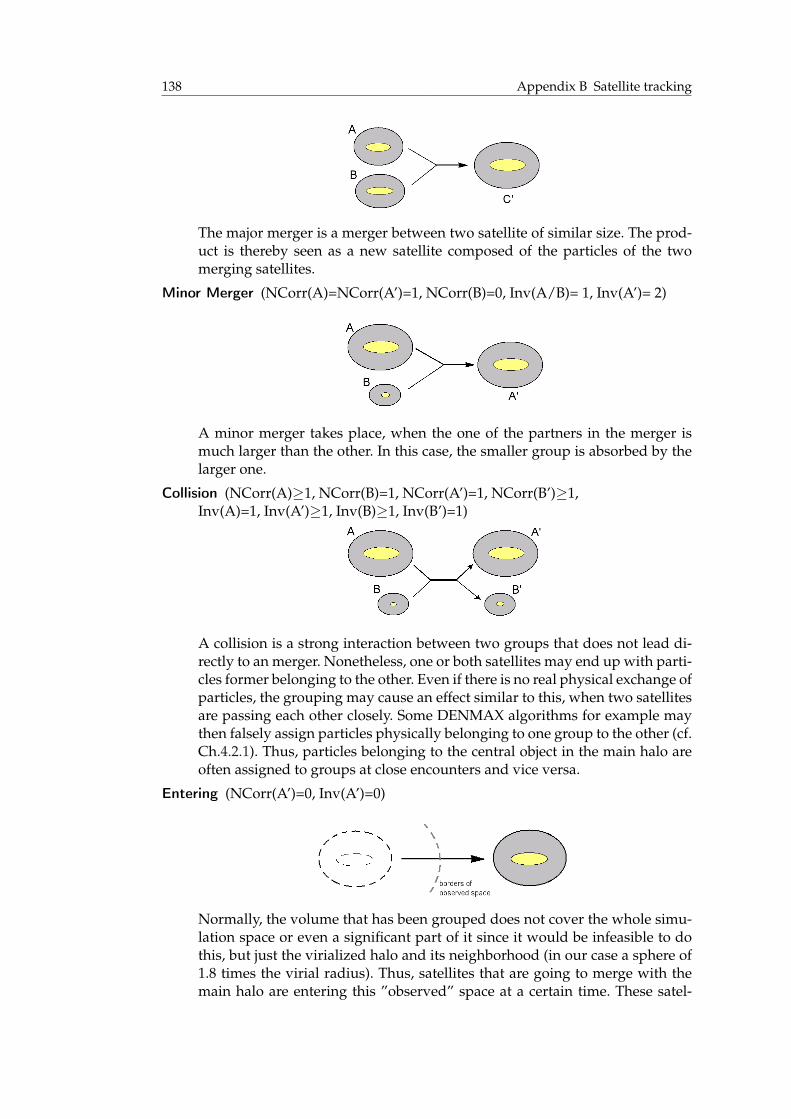
138 Appendix B Satellite tracking
The major merger is a merger between two satellite of similar size. The prod-uct is thereby seen as a new satellite composed of the particles of the twomerging satellites.
Minor Merger (NCorr(A)=NCorr(A’)=1, NCorr(B)=0, Inv(A/B)= 1, Inv(A’)= 2)
A minor merger takes place, when the one of the partners in the merger ismuch larger than the other. In this case, the smaller group is absorbed by thelarger one.
Collision (NCorr(A)≥1, NCorr(B)=1, NCorr(A’)=1, NCorr(B’)≥1,Inv(A)=1, Inv(A’)≥1, Inv(B)≥1, Inv(B’)=1)
A collision is a strong interaction between two groups that does not lead di-rectly to an merger. Nonetheless, one or both satellites may end up with parti-cles former belonging to the other. Even if there is no real physical exchange ofparticles, the grouping may cause an effect similar to this, when two satellitesare passing each other closely. Some DENMAX algorithms for example maythen falsely assign particles physically belonging to one group to the other (cf.Ch.4.2.1). Thus, particles belonging to the central object in the main halo areoften assigned to groups at close encounters and vice versa.
Entering (NCorr(A’)=0, Inv(A’)=0)
Normally, the volume that has been grouped does not cover the whole simu-lation space or even a significant part of it since it would be infeasible to dothis, but just the virialized halo and its neighborhood (in our case a sphere of1.8 times the virial radius). Thus, satellites that are going to merge with themain halo are entering this ”observed” space at a certain time. These satel-

B.1 Cases 139
lites thereby consist (mostly) of particles that have not been in the observedvolume the snapshot before (for re-entering see ”Leaving”).
Leaving (NCorr(A)=1, Inv(A)=1) 68
As mentioned for the ”Entering” case, the part of simulation volume that wegrouped is usually restricted to the direct neighborhood of the main halo.Thus, it is possible that satellites may enter this space and leave again, if theyhave not already lost to much energy by e.g. dynamical friction. Being un-able to track them outside, since this space is not grouped, we may keep theparticles belonging to them marked, such that the satellites can be recognizedif they re-enter the observed space. This allows us to distinguish them fromsatellites that enter the first time.
Border (NCorr(A)=2, Inv(A)=2, NCorr(A’) = 1, Inv(A’) = 1)
Besides of having to deal with re-entering satellites, another problem ariseswith the bounded observed space. When a satellite is entering or leaving thisspace and a snapshot is taken just at that moment, we observe in the case of re-entering a satellite that is only a fragment of the satellite that has been left andwho seems to merges with another satellite incoming satellite just the nextsnapshot (which is in fact the part of the satellite that has been outside at thesnapshot of the entering). A similar effect is observed for leaving satellites.To solve this, the satellite is not split up instantly if a significant part is notin the observed volume. This process is delayed for one snapshot, at whichthe satellite has either fully entered or left the observed space (whereas weassume that the time period between two snapshots is large enough comparedto the velocity and size of the satellites).
Lost (NCorr(A) = 0, Inv(A) = 0)
If a particles of group A do not end up in a significant amount in any group,this group is assumed to be no longer existent, i.e. the satellites was totallydisrupted or at least too small for the grouping mechanism to be detected.Similar to the Merger and Split-up case, this classification is implemented to
68The (sub)set of particles of a satellite that left the observed space is treated as an additional group

140 Appendix B Satellite tracking
be delayed for one snapshots to overcome a possible one-time failure of thegrouping.
(Splitting up) (NCorr(A)= 2, NCorr(B’/C’)= 1, Inv(A)= 2, Inv(B’/C’)= 1)
In the ”physical” universe it is rather unlikely that non-rigid objects like satel-lites suddenly split up into two or more rather larger parts instead of beingtotally disrupted by the process. But this can sometimes happen as a groupingartifact, where the particles of a groups seem to end up in two distinct groups.Thus, this case rather provides a mean to fix this wrong grouping by delayingthe split-up of the tracking of the satellite into two new groups for at least onesnapshot.
B.2 Algorithm
After having presented the situations a satellite can face, we now want to discussthe algorithm, in particular the decision tree on which the final result is based.Given two snapshots S and S′, the algorithm consists of the following steps to per-form the tracking:
1. Calculation of Corr(A, B′) and Inv(A, B′) for all groups A in S and B′ in S′.
2. Calculation of NCorr(A) and NInv(A) for all groups A in S and S′.
3. Classifying satellites in S′ based on the decision tree shown in Fig.70.
4. Assign the groups in S′ to the already known satellites in case of a one-to-onerelationship to a group in S and add groups that have been seen the first time,are product of mergers or too small remnants of a former satellite to the list ofknown satellites.
5. Checking the groups of S that have not been associated with any group in S′
in the step before. Check if they have been either left or lost.
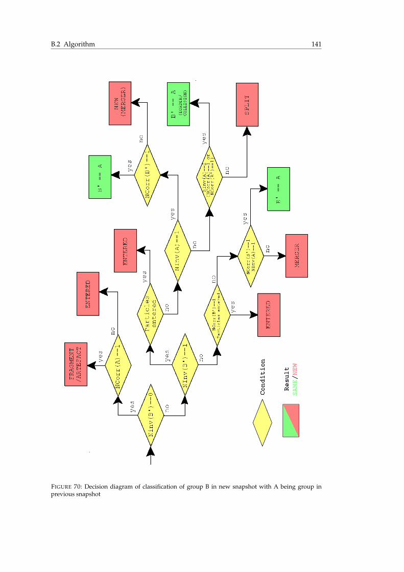
B.2 Algorithm 141
FIGURE 70: Decision diagram of classification of group B in new snapshot with A being group inprevious snapshot


APPENDIX C
PLOTS / RESULTS
This chapter provides all the plots of the chapters in the evaluation part that hadbeen referred to, but had not been shown there due to lack of space.
C.1 Evaluation/Comparison of Galaxy Halos
100
120
140
160
180
200
220
0 0.5 1 1.5 2 2.5 3 3.5 4
Rvi
r,co
m [k
pc/h
]
Redshift z
Gal0
DMDM
HydroHydro
100
120
140
160
180
200
220
0 0.5 1 1.5 2 2.5 3
Rvi
r,co
m [k
pc/h
]
Redshift z
Gal1
DMDM
HydroHydro
170
180
190
200
210
220
230
0 0.5 1 1.5 2
Rvi
r,co
m [k
pc/h
]
Redshift z
Gal3
DMDM
HydroHydro
FIGURE 71: Evolution of Rvir of main halo in Gal0, Gal1, Gal3
143

144 Appendix C Plots / Results
1000
10000
100000
1e+06ρ 0
[I.U
.]
Gal0
DMHydro
1
10
100
Rs
[kpc
/h]
DMHydro
1000
10000
100000
0 0.2 0.4 0.6 0.8 1 1.2 1.4
χ2 /dof
redshift z
DMHydro
100
1000
10000
100000
1e+06
ρ 0 [I
.U.]
Gal1
DMHydro
1
10
100
Rs
[kpc
/h]
DMHydro
1000
10000
100000
1e+06
0 0.5 1 1.5 2
χ2 /dof
redshift z
DMHydro
1000
10000
100000
1e+06
ρ 0 [I
.U.]
Gal3
DMHydro
1
10
100
Rs
[kpc
/h]
DMHydro
1000
10000
100000
1e+06
0 0.5 1 1.5 2
χ2 /dof
redshift z
DMHydro
FIGURE 72: Evolution of Main Halo in Gal0, Gal1, Gal3 based on NFW density profile fits
1 10
100 1000
10000 100000 1e+06
ρ 0 [I
.U.]
Gal0
DMHydro
1
10
100
1000
Rs
[kpc
/h]
DMHydro
0.01
0.1
1
10
γ
DMHydro
1000
10000
100000
0 0.2 0.4 0.6 0.8 1 1.2 1.4
χ2 /dof
redshift z
DMHydro
1e-06 0.0001
0.01 1
100 10000 1e+06 1e+08 1e+10 1e+12
ρ 0 [I
.U.]
Gal1
DMHydro
0.1 1
10 100
1000 10000
100000 1e+06
Rs
[kpc
/h]
DMHydro
0.1
1
10
γ
DMHydro
1000
10000
100000
1e+06
0 0.5 1 1.5 2
χ2 /dof
redshift z
DMHydro
0.01 0.1
1 10
100 1000
10000 100000
ρ 0 [I
.U.]
Gal3
DMHydro
10
100
1000
10000
Rs
[kpc
/h]
DMHydro
0.1
1
10
γ
DMHydro
1000
10000
100000
0 0.5 1 1.5 2
χ2 /dof
redshift z
DMHydro
FIGURE 73: Evolution of Main Halo in Gal0, Gal1, Gal3 based on GNFW density profile fits

C.1 Evaluation/Comparison of Galaxy Halos 145
1e-05
0.0001
0.001
ρ 0 [I
.U.]
Gal0
DMHydro
10000
100000
1e+06
0 0.2 0.4 0.6 0.8 1 1.2 1.4
χ2 /dof
redshift z
DMHydro
1e-05
0.0001
0.001
ρ 0 [I
.U.]
Gal1
DMHydro
10000
100000
1e+06
0 0.5 1 1.5 2
χ2 /dof
redshift z
DMHydro
1e-05
0.0001
0.001
ρ 0 [I
.U.]
Gal3
DMHydro
10000
100000
1e+06
0 0.5 1 1.5 2
χ2 /dof
redshift z
DMHydro
FIGURE 74: Evolution of Main Halo in Gal0, Gal1, Gal3 based on SIS density profile fits
0.01
0.1
1
γ
Gal0
DMHydro
0.001
0.01
0.1
1
10
100
R-2
[kpc
/h]
DMHydro
100 1000
10000 100000 1e+06 1e+07 1e+08 1e+09 1e+10
ρ -2
[I.U
.]
DMHydro
100
1000
10000
100000
0 0.2 0.4 0.6 0.8 1 1.2 1.4
χ2 /dof
redshift z
DMHydro
0.001
0.01
0.1
1
γ
Gal1
DMHydro
0.01
0.1
1
10
100
R-2
[kpc
/h]
DMHydro
10 100
1000 10000
100000 1e+06 1e+07 1e+08 1e+09 1e+10 1e+11
ρ -2
[I.U
.]
DMHydro
1000
10000
100000
0 0.5 1 1.5 2
χ2 /dof
redshift z
DMHydro
0.001
0.01
0.1
1
γ
Gal3
DMHydro
1e-05 0.0001
0.001 0.01
0.1 1
10 100
R-2
[kpc
/h]
DMHydro
100 10000 1e+06 1e+08 1e+10 1e+12 1e+14 1e+16
ρ -2
[I.U
.]
DMHydro
1000
10000
100000
0 0.5 1 1.5 2
χ2 /dof
redshift z
DMHydro
FIGURE 75: Evolution of Main Halo in Gal0, Gal1, Gal3 based on PoLLs density profile fits

146 Appendix C Plots / Results
1000
10000
100000
1e+06
1e+07
1e+08
1e+09
1e+10
1e+11
1e+12
0.01 0.1 1
ρ(r)
/ M
Hal
o [I.
U.]
r / Rvir
Gal0
total z=0Gas z=0
Stars z=0total z=1Gas z=1
Stars z=1
1000
10000
100000
1e+06
1e+07
1e+08
1e+09
1e+10
1e+11
1e+12
0.01 0.1 1
ρ(r)
/ M
Hal
o [I.
U.]
r / Rvir
Gal3
total z=0Gas z=0
Stars z=0total z=1Gas z=1
Stars z=1
FIGURE 76: Density profiles of gas, star and total matter at redshifts z = 0 and z = 1
0
0.01
0.02
0.03
0.04
0.05
0 2 4 6 8 10 12 14
ρ / ρ
crit
age of universe [Gyr]
Gal0
GasStars
z=1
0
0.01
0.02
0.03
0.04
0.05
0 2 4 6 8 10 12 14
ρ / ρ
crit
age of universe [Gyr]
Gal1
GasStars
z=1
0
0.01
0.02
0.03
0.04
0.05
0 2 4 6 8 10 12 14
ρ / ρ
crit
age of universe [Gyr]
Gal3
GasStars
z=1
FIGURE 77: Evolution of star and gas matter density in Universe

C.1 Evaluation/Comparison of Galaxy Halos 147
5e+11
6e+11
7e+11
8e+11
9e+11
1e+12
1.1e+12
0 0.2 0.4 0.6 0.8 1 1.2 1.4
MH
alo
[MO•
]
redshift z
DMHydro
0
2e+11
4e+11
6e+11
8e+11
1e+12
1.2e+12
1.4e+12
0 0.5 1 1.5 2 2.5
MH
alo
[MO•
]
redshift z
DMHydro
4e+11
5e+11
6e+11
7e+11
8e+11
9e+11
1e+12
1.1e+12
1.2e+12
1.3e+12
1.4e+12
0 0.5 1 1.5 2
MH
alo
[MO•
]
redshift z
DMHydro
FIGURE 78: Comparison of mass evolution for same main halo in DM and Hydro simulation
0
2e+11
4e+11
6e+11
8e+11
1e+12
1.2e+12
1.4e+12
1.6e+12
1.8e+12
0 0.2 0.4 0.6 0.8 1 1.2 1.4
M(<
r) [M
O•]
redshift z
Gal0
DM rcom=900kpcHydro rcom=900kpc
DM rcom=450kpcHydro rcom=450kpc
DM rcom=90kpcHydro rcom=90kpc
0
2e+11
4e+11
6e+11
8e+11
1e+12
1.2e+12
1.4e+12
1.6e+12
1.8e+12
2e+12
0 0.2 0.4 0.6 0.8 1 1.2 1.4
M(<
r) [M
O•]
redshift z
Gal1
DM rcom=900kpcHydro rcom=900kpc
DM rcom=450kpcHydro rcom=450kpc
DM rcom=90kpcHydro rcom=90kpc
2e+11
4e+11
6e+11
8e+11
1e+12
1.2e+12
1.4e+12
1.6e+12
1.8e+12
2e+12
2.2e+12
0 0.2 0.4 0.6 0.8 1 1.2 1.4
M(<
r) [M
O•]
redshift z
Gal3
DM rcom=900kpcHydro rcom=900kpc
DM rcom=450kpcHydro rcom=450kpc
DM rcom=90kpcHydro rcom=90kpc
FIGURE 79: Comparison of mass evolution around main halo in DM and Hydro simulation

148 Appendix C Plots / Results
0
5e+10
1e+11
1.5e+11
2e+11
2.5e+11
3e+11
3.5e+11
4e+11
4.5e+11
5e+11
0 0.2 0.4 0.6 0.8 1 1.2 1.4
M(<
r com
=90
kpc)
[MO•
]
redshift z
Gal0
DM res.3Hydro res.3
DM res.4Hydro res.4
DM converted baryonicHydro baryonic
0
1e+11
2e+11
3e+11
4e+11
5e+11
6e+11
0 0.2 0.4 0.6 0.8 1 1.2 1.4
M(<
r com
=90
kpc)
[MO•
]
redshift z
Gal1
DM res.3Hydro res.3
DM res.4Hydro res.4
DM converted baryonicHydro baryonic
0
1e+11
2e+11
3e+11
4e+11
5e+11
6e+11
0 0.2 0.4 0.6 0.8 1 1.2 1.4
M(<
r com
=90
kpc)
[MO•
]
redshift z
Gal3
DM res.3Hydro res.3
DM res.4Hydro res.4
DM converted baryonicHydro baryonic
FIGURE 80: Comparison of mass evolution in sphere of radius rcom = 90kpc around main halo in DMand Hydro simulation
0
1e+11
2e+11
3e+11
4e+11
5e+11
6e+11
7e+11
8e+11
9e+11
1e+12
0 0.2 0.4 0.6 0.8 1 1.2 1.4
M(<
r com
=27
0kpc
) [M
O•]
redshift z
Gal1
DM res.3Hydro res.3
DM res.4Hydro res.4
DM converted baryonicHydro baryonic
0
1e+11
2e+11
3e+11
4e+11
5e+11
6e+11
7e+11
8e+11
9e+11
1e+12
0 0.2 0.4 0.6 0.8 1 1.2 1.4
M(<
r com
=27
0kpc
) [M
O•]
redshift z
Gal3
DM res.3Hydro res.3
DM res.4Hydro res.4
DM converted baryonicHydro baryonic
FIGURE 81: Comparison of mass evolution in sphere of radius rcom = 270kpc around main halo inDM and Hydro simulation

C.1 Evaluation/Comparison of Galaxy Halos 149
0
1e+11
2e+11
3e+11
4e+11
5e+11
6e+11
7e+11
8e+11
9e+11
1e+12
0 0.2 0.4 0.6 0.8 1 1.2 1.4
M(<
r com
=45
0kpc
) [M
O•]
redshift z
Gal0
DM res.3Hydro res.3
DM res.4Hydro res.4
DM converted baryonicHydro baryonic
0
2e+11
4e+11
6e+11
8e+11
1e+12
1.2e+12
0 0.2 0.4 0.6 0.8 1 1.2 1.4
M(<
r com
=45
0kpc
) [M
O•]
redshift z
Gal1
DM res.3Hydro res.3
DM res.4Hydro res.4
DM converted baryonicHydro baryonic
0
2e+11
4e+11
6e+11
8e+11
1e+12
1.2e+12
0 0.2 0.4 0.6 0.8 1 1.2 1.4
M(<
r com
=45
0kpc
) [M
O•]
redshift z
Gal3
DM res.3Hydro res.3
DM res.4Hydro res.4
DM converted baryonicHydro baryonic
FIGURE 82: Comparison of mass evolution in sphere of radius rcom = 450kpc around main halo inDM and Hydro simulation
0
1e+11
2e+11
3e+11
4e+11
5e+11
6e+11
7e+11
8e+11
9e+11
1e+12
0 0.2 0.4 0.6 0.8 1 1.2 1.4
M(<
r com
=90
0kpc
) [M
O•]
redshift z
Gal0
DM res.3Hydro res.3
DM res.4Hydro res.4
DM converted baryonicHydro baryonic
0
2e+11
4e+11
6e+11
8e+11
1e+12
1.2e+12
0 0.2 0.4 0.6 0.8 1 1.2 1.4
M(<
r com
=90
0kpc
) [M
O•]
redshift z
Gal3
DM res.3Hydro res.3
DM res.4Hydro res.4
DM converted baryonicHydro baryonic
FIGURE 83: Comparison of mass evolution in sphere of radius rcom = 900kpc around main halo inDM and Hydro simulation

150 Appendix C Plots / Results
C.2 Comparison of Satellite ”twins”
0.4
0.6
0.8
1
1.2
1.4
1.6
1.8
2
-0.2 0 0.2 0.4 0.6 0.8 1 1.2
r/r v
ir
redshift z
Gal0 DM Group 179, Hydro Group 102 (rel.) Distance to Galaxy
distance to center dmdistance to center hydro
0.4
0.5
0.6
0.7
0.8
0.9
1
1.1
1.2
-0.2 0 0.2 0.4 0.6 0.8 1 1.2
reta
ined
mas
s M
sat(z
)/M
infa
ll
redshift z
Gal0 DM Group 179, Hydro Group 102 (rel.) Distance to Galaxy
mass dmmass hydro
0
0.2
0.4
0.6
0.8
1
1.2
1.4
1.6
1.8
2
-0.2 0 0.2 0.4 0.6 0.8 1 1.2
r/r v
ir
redshift z
Gal0 DM Group 220, Hydro Group 101 (rel.) Distance to Galaxy
distance to center dmdistance to center hydro
0.4
0.5
0.6
0.7
0.8
0.9
1
1.1
-0.2 0 0.2 0.4 0.6 0.8 1 1.2
reta
ined
mas
s M
sat(z
)/M
infa
ll
redshift z
Gal0 DM Group 220, Hydro Group 101 (rel.) Distance to Galaxy
mass dmmass hydro
0.2
0.4
0.6
0.8
1
1.2
1.4
1.6
1.8
2
-0.1 0 0.1 0.2 0.3 0.4 0.5 0.6 0.7 0.8 0.9 1
r/r v
ir
redshift z
Gal0 DM Group 225, Hydro Group 128 (rel.) Distance to Galaxy
distance to center dmdistance to center hydro
0.4
0.5
0.6
0.7
0.8
0.9
1
1.1
-0.1 0 0.1 0.2 0.3 0.4 0.5 0.6 0.7 0.8 0.9 1
reta
ined
mas
s M
sat(z
)/M
infa
ll
redshift z
Gal0 DM Group 225, Hydro Group 128 (rel.) Distance to Galaxy
mass dmmass hydro
0
0.2
0.4
0.6
0.8
1
1.2
1.4
1.6
1.8
2
-0.2 0 0.2 0.4 0.6 0.8 1 1.2 1.4 1.6
r/r v
ir
redshift z
Gal0 DM Group 134, Hydro Group 104 (rel.) Distance to Galaxy
distance to center dmdistance to center hydro
0.4
0.5
0.6
0.7
0.8
0.9
1
1.1
-0.2 0 0.2 0.4 0.6 0.8 1 1.2 1.4 1.6 0.4
0.5
0.6
0.7
0.8
0.9
1
1.1
rel.
dist
ance
r/R
vir
reta
ined
mas
s M
sat(z
)/M
infa
ll
redshift z
Gal0 DM Group 134, Hydro Group 104 (rel.) Distance to Galaxy
mass dmmass hydro
FIGURE 84: Satellites that lost less mass in the hydrodynamical simulation than in the pure DM sim-ulation

C.2 Comparison of Satellite ”twins” 151
0
0.2
0.4
0.6
0.8
1
1.2
1.4
1.6
1.8
2
-0.1 0 0.1 0.2 0.3 0.4 0.5 0.6 0.7
r/r v
ir
redshift z
Gal0 DM Group 330, Hydro Group 155 (rel.) Distance to Galaxy
distance to center dmdistance to center hydro
0
0.2
0.4
0.6
0.8
1
1.2
-0.1 0 0.1 0.2 0.3 0.4 0.5 0.6 0.7
reta
ined
mas
s M
sat(z
)/M
infa
ll
redshift z
Gal0 DM Group 330, Hydro Group 155 (rel.) Distance to Galaxy
mass dmmass hydro
0
0.2
0.4
0.6
0.8
1
1.2
1.4
1.6
1.8
2
-0.2 0 0.2 0.4 0.6 0.8 1 1.2
r/r v
ir
redshift z
Gal1 DM Group 351, Hydro Group 214 (rel.) Distance to Galaxy
distance to center dmdistance to center hydro
0.2
0.3
0.4
0.5
0.6
0.7
0.8
0.9
1
1.1
-0.2 0 0.2 0.4 0.6 0.8 1 1.2
reta
ined
mas
s M
sat(z
)/M
infa
ll
redshift z
Gal1 DM Group 351, Hydro Group 214 (rel.) Distance to Galaxy
mass dmmass hydro
0.2
0.4
0.6
0.8
1
1.2
1.4
1.6
1.8
2
-0.1 0 0.1 0.2 0.3 0.4 0.5 0.6 0.7 0.8 0.9 1
r/r v
ir
redshift z
Gal1 DM Group 413, Hydro Group 234 (rel.) Distance to Galaxy
distance to center dmdistance to center hydro
0.3
0.4
0.5
0.6
0.7
0.8
0.9
1
1.1
-0.1 0 0.1 0.2 0.3 0.4 0.5 0.6 0.7 0.8 0.9 1
reta
ined
mas
s M
sat(z
)/M
infa
ll
redshift z
Gal1 DM Group 413, Hydro Group 234 (rel.) Distance to Galaxy
mass dmmass hydro
0.2
0.4
0.6
0.8
1
1.2
1.4
1.6
1.8
2
-0.2 0 0.2 0.4 0.6 0.8 1 1.2
r/r v
ir
redshift z
Gal1 DM Group 310, Hydro Group 169 (rel.) Distance to Galaxy
distance to center dmdistance to center hydro
0.2
0.4
0.6
0.8
1
1.2
1.4
1.6
-0.2 0 0.2 0.4 0.6 0.8 1 1.2
reta
ined
mas
s M
sat(z
)/M
infa
ll
redshift z
Gal1 DM Group 310, Hydro Group 169 (rel.) Distance to Galaxy
mass dmmass hydro
0.2
0.4
0.6
0.8
1
1.2
1.4
1.6
1.8
2
-0.2 0 0.2 0.4 0.6 0.8 1 1.2
r/r v
ir
redshift z
Gal1 DM Group 313, Hydro Group 199 (rel.) Distance to Galaxy
distance to center dmdistance to center hydro
0.5
0.55
0.6
0.65
0.7
0.75
0.8
0.85
0.9
0.95
1
1.05
-0.2 0 0.2 0.4 0.6 0.8 1 1.2
reta
ined
mas
s M
sat(z
)/M
infa
ll
redshift z
Gal1 DM Group 313, Hydro Group 199 (rel.) Distance to Galaxy
mass dmmass hydro
FIGURE 85: Satellites that lost more mass in the hydrodynamical simulation than in the pure DMsimulation
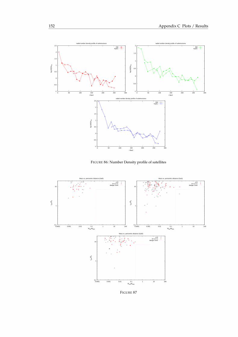
152 Appendix C Plots / Results
-1
-0.5
0
0.5
1
1.5
2
2.5
0 50 100 150 200 250 300
log
N(R
)/n v
ir
r [kpc]
radial number density profile of substructures
DMHydro
-1
-0.5
0
0.5
1
1.5
2
0 50 100 150 200 250 300
log
N(R
)/n v
ir
r [kpc]
radial number density profile of substructures
DMHydro
-1
-0.5
0
0.5
1
1.5
2
2.5
0 50 100 150 200 250 300
log
N(R
)/n v
ir
r [kpc]
radial number density profile of substructures
DMHydro
FIGURE 86: Number Density profile of satellites
0.1
1
10
0.0001 0.001 0.01 0.1 1 10 100
r per
i/Rd
Msat/Mdisk
Mass vs. pericentric distance (Gal0)
z=00<=z<=1
danger zone
0.1
1
10
0.0001 0.001 0.01 0.1 1 10 100
r per
i/Rd
Msat/Mdisk
Mass vs. pericentric distance (Gal1)
z=00<=z<=1
danger zone
0.1
1
10
0.0001 0.001 0.01 0.1 1 10 100
r per
i/Rd
Msat/Mdisk
Mass vs. pericentric distance (Gal3)
z=00<=z<=1
danger zone
FIGURE 87

C.2 Comparison of Satellite ”twins” 153
0.1
1
10
0.0001 0.001 0.01 0.1 1 10 100
r per
i/Rd
Msat/Mdisk
Mass vs. pericentric distance (Gal0)
z=00<=z<=1
danger zone
0.1
1
10
0.0001 0.001 0.01 0.1 1 10 100
r per
i/Rd
Msat/Mdisk
Mass vs. pericentric distance (Gal1)
z=00<=z<=1
danger zone
0.1
1
10
0.0001 0.001 0.01 0.1 1 10 100
r per
i/Rd
Msat/Mdisk
Mass vs. pericentric distance (Gal3)
z=00<=z<=1
danger zone
FIGURE 88
0.1
1
10
0.0001 0.001 0.01 0.1 1 10 100
r per
i/Rd
Msat/Mdisk
Mass vs. pericentric distance (Gal0)
DM z=0Hydro z=0
DM 0<=z<=1Hydro 0<=z<=1
danger zone
0.1
1
10
0.0001 0.001 0.01 0.1 1 10 100
r per
i/Rd
Msat/Mdisk
Mass vs. pericentric distance (Gal1)
DM z=0Hydro z=0
DM 0<=z<=1Hydro 0<=z<=1
danger zone
0.1
1
10
0.0001 0.001 0.01 0.1 1 10 100
r per
i/Rd
Msat/Mdisk
Mass vs. pericentric distance (Gal3)
DM z=0Hydro z=0
DM 0<=z<=1Hydro 0<=z<=1
danger zone
FIGURE 89: Scatter plot of pericentric distance versus satellite mass. Filled symbols thereby representthe satellites that cross within a radius of 50 kpc after z = 1 while unfilled symbols mark the propertiesof surviving substructures at z = 0

154 Appendix C Plots / Results
0
0.2
0.4
0.6
0.8
1
1.2
1.4
1.6
0 0.2 0.4 0.6 0.8 1 1.2 1.4
r/R
vir
redshift z
Group 243 (rel.) Distance to Galaxy
distance to center(extrapol.) periapsis distance
0
0.2
0.4
0.6
0.8
1
1.2
1.4
1.6
0 0.2 0.4 0.6 0.8 1 1.2 1.4 0
0.2
0.4
0.6
0.8
1
1.2
1.4
rel.
dist
ance
r/R
vir
reta
ined
mas
s M
sat(z
)/M
infa
ll
redshift z
Group 243 (rel.) Distance to Galaxy
distancemass
0
0.2
0.4
0.6
0.8
1
1.2
1.4
1.6
0 0.2 0.4 0.6 0.8 1 1.2 1.4 0
0.2
0.4
0.6
0.8
1
1.2
1.4
1.6
M(z
)/M
(zin
fall=
1.1)
reta
ined
mas
s M
sat(z
)/M
infa
ll
redshift z
Group 243: (rel.) retained Mass
totalgasDM
stars
FIGURE 90: Evolution of a hydrodynamical satellite.

C.2 Comparison of Satellite ”twins” 155
1
10
100
1000
10000
100000
1e+06
1 10
Den
sity
ρ(r
)
r [kpc/h]
total z=1.3total z=1.0
total z=0Baryonic z=1.3Baryonic z=1.0
Baryonic z=0
FIGURE 91: Evolution of the density profiles of seperate components of halo shown in Fig.90
-8
-6
-4
-2
0
2
4
0 0.2 0.4 0.6 0.8 1 1.2 1.4 1.6
t Infa
ll,dm
-tIn
fall,
hydr
o[G
yr]
zInfall,dm
Gal0Gal1Gal3
FIGURE 92: Comparison of infall times


VERSICHERUNG
Versicherung gemäß Paragraph 18, Absatz 7 der Diplomprüfungsordnung für denStudiengang Physik an der Physik Fakultät der Universität Bielefeld vom 10. Jan-uar 1996.
Hiermit versichere ich, daß ich die vorliegende Diplomarbeit selbständig erarbeitetund keine anderen als die angegebenen Quellen und Hilfsmittel benutzt sowie Zi-tate kenntlich gemacht habe.
Bielefeld, Mai 2010


![[standard] Baryonic Acoustic Oscillations (BAO), Redshift ... · [standard] Baryonic Acoustic Oscillations (BAO), Redshift Space Distortions (RSD), and some (renewed) ideas... Carlo](https://img.dokumen.tips/doc/110x75/5f0c7c127e708231d435a2a6/standard-baryonic-acoustic-oscillations-bao-redshift-standard-baryonic.jpg)