Embed Size (px)
Citation preview

Introductory Machine LearningNotes1
Lorenzo RosascoDIBRIS, Universita’ degli Studi di Genova
LCSL, Massachusetts Institute of Technology and Istituto Italiano di
October 10, 2016
1
These notes are an attempt to extract essential machine learning concepts for be-ginners. They are a draft and will be updated. Likely they won’t be typos free fora while. They are dry and lack examples to complement and illustrate the generalideas. Notably, they also lack references, that will (hopefully) be added soon. Themathematical appendix is due to Andre Wibisono’s notes for the math camp of the9.520 course at MIT.

ABSTRACT. Machine Learning has become a key to develop intel-ligent systems and analyze data in science and engineering. Ma-chine learning engines enable systems such as Siri, Kinect or theGoogle self driving car, to name a few examples. At the same timemachine learning methods help deciphering the information inour DNA and make sense of the flood of information gathered onthe web. These notes provide an introduction to the fundamentalconcepts and methods at the core of modern machine learning.

Contents
Chapter 1. Statistical Learning Theory 11.1. Data 11.2. Probabilistic Data Model 11.3. Loss Function and and Expected Risk 31.4. Stability, Overfitting and Regularization 4
Chapter 2. Local Methods 52.1. Nearest Neighbor 52.2. K-Nearest Neighbor 62.3. Parzen Windows 72.4. High Dimensions 8
Chapter 3. Bias Variance and Cross-Validation 93.1. Tuning and Bias Variance Decomposition 93.2. The Bias Variance Trade-Off 103.3. Cross Validation 10
Chapter 4. Regularized Least Squares 134.1. Regularized Least Squares 134.2. Computations 144.3. Interlude: Linear Systems 144.4. Dealing with an Offset 15
Chapter 5. Regularized Least Squares Classification 175.1. Nearest Centroid Classifier 175.2. RLS for Binary Classification 185.3. RLS for Multiclass Classification 19
Chapter 6. Feature, Kernels and Representer Theorem 216.1. Feature Maps 216.2. Representer Theorem 226.3. Kernels 23
Chapter 7. Regularization Networks 257.1. Empirical Risk Minimization 257.2. Hypotheses Space 25
iii

iv CONTENTS
7.3. Tikhonov Regularization and Representer Theorem 267.4. Loss Functions and Target Functions 27
Chapter 8. Logistic Regression 298.1. Interlude: Gradient Descent and Stochastic Gradient 298.2. Regularized Logistic Regression 318.3. Kernel Regularized Logistic Regression 328.4. Logistic Regression and Confidence Estimation 32
Chapter 9. From Perceptron to SVM 339.1. Perceptron 339.2. Margin 339.3. Maximizing the Margin 359.4. From Max Margin to Tikhonov Regularization 369.5. Computations 369.6. Dealing with an off-set 36
Chapter 10. Dimensionality Reduction 3710.1. PCA & Reconstruction 3810.2. PCA and Maximum Variance 3810.3. PCA and Associated Eigenproblem 3910.4. Beyond the First Principal Component 3910.5. Singular Value Decomposition 4010.6. Kernel PCA 41
Chapter 11. Variable Selection 4311.1. Subset Selection 4311.2. Greedy Methods: (Orthogonal) Matching Pursuit 4411.3. Convex Relaxation: LASSO & Elastic Net 45
Chapter 12. A Glimpse Beyond The Fence 4912.1. Different Kinds of Data 4912.2. Data and Sampling Models 5012.3. Learning Approaches 5012.4. Some Current and Future Challenges in Machine
Learning 50
Appendix A. Mathematical Tools 53A.1. Structures on Vector Spaces 53A.2. Matrices 56

CHAPTER 1
Statistical Learning Theory
Machine Learning deals with systems that are trained from datarather than being explicitly programmed. Here we describe the datamodel considered in statistical learning theory.
1.1. Data
The goal of supervised learning is to find an underlying input-outputrelation
f(xnew) ∼ y,
given data.The data, called training set, is a set of n input-output pairs,
S = (x1, y1), . . . , (xn, yn).Each pair is called an example or sample, or data point. We considerthe approach to machine learning based on the so called learning fromexamples paradigm.
Given the training set, the goal is to learn a corresponding input-output relation. To make sense of this task, we have to postulatethe existence of a model for the data. The model should take intoaccount the possible uncertainty in the task and in the data.
1.2. Probabilistic Data Model
The inputs belong to an input space X , we assume throughoutthat X ⊆ RD. The outputs belong to an output space Y . We con-sider several possible situations: regression Y ⊆ R, binary classi-fication Y = −1, 1 and multi-category (multiclass) classificationY = 1, 2, . . . , T. The space X × Y is called the data space.
We assume there exists a fixed unknown data distribution p(x, y)according to which the data are identically and independently dis-tributed (i.i.d.) 1. The probability distribution p models differentsources of uncertainty. We assume that it factorizes as p(x, y) =pX(x)p(y|x), where
1the examples are sampled independently from the same probability distribu-tion p
1

2 1. STATISTICAL LEARNING THEORY
• the conditional distribution p(y|x), see Figure 1, describes anon deterministic relation between input and output.• The marginal distribution pX(x) models uncertainty in the
sampling of the input points.We provide two classical examples of data model, namely regressionand classification.
EXAMPLE 1 (Regression). In regression the following model is oftenconsidered y = f ∗(x)+ε.Here f ∗ is a fixed unknown function, for examplea linear function f ∗(x) = xTw∗ for some w∗ ∈ RD and ε is random noise,e.g. standard Gaussian N (0, σ), σ ∈ [0,∞). See Figure 2 for an example.
EXAMPLE 2 (Classification). In binary classification a basic exam-ple of data model is a mixture of two Gaussians, i.e. p(x|y = −1) =1ZN (−1, σ−), σ− ∈ [0,∞) and p(x|y = 1) = 1
ZN (+1, σ+), σ+ ∈ [0,∞),
where 1Z
is a suitable normalization. For example in classification, a noise-less situation corresponds to p(1|x) = 1 or 0 for all x.
YX
p (y|x)
x
FIGURE 1. For each input x there is a distribution ofpossible outputs p(y|x) (yellow). The green area is thedistribution of all possible outputs.
FIGURE 2. Fixed unknown linear function f ∗ andnoisy examples sampled from the y = f ∗(x) + ε model.

1.3. LOSS FUNCTION AND AND EXPECTED RISK 3
-3 -2 -1 0 1 2 3-2
-1.5
-1
-0.5
0
0.5
1
1.5
2
FIGURE 3. 2D example of a dataset sampled from amixed Gaussian distribution. Samples of the yellowclass are realizations of a Gaussian centered at (−1, 0),while samples of the blue class are realizations of aGaussian centered at (+1, 0). Both Gaussians havestandard deviation σ = 0.6.
1.3. Loss Function and and Expected Risk
The goal of learning is to estimate the “best” input-output rela-tion, rather than the whole distribution p.
More precisely, we need to fix a loss function
` : Y × Y → [0,∞),
which is a (point-wise) measure of the error `(y, f(x)) we incur inwhen predicting f(x) in place of y. Given a loss function, the ”best”input-output relation is the target function f ∗ : X → Y minimizingthe expected loss (or expected risk)
E(f) = E[`(y, f(x))] =
∫dxdyp(x, y)`(y, f(x)).
which can be seen as a measure of the error on past as well as futuredata. The target function cannot be computed since the probabilitydistribution p is unknown. A (good) learning algorithm should pro-vide a solution that behaves similarly to the target function, and pre-dict/classify well new data. In this case, we say that the algorithmgeneralizes.
REMARK 1 (Decision Surface/Boundary). In classification we of-ten visualize the so called decision boundary (or surface) of a classificationsolution f . The decision boundary is the level set of points x for whichf(x) = 0.

4 1. STATISTICAL LEARNING THEORY
1.4. Stability, Overfitting and Regularization
A learning algorithm is a procedure that given a training set S com-putes an estimator fS . Ideally, an estimator should mimic the targetfunction, in the sense that E(fS) ≈ E(f ∗). The latter requirementneeds some care since fS depends on the training set and hence israndom. For example, one possibility is to require an algorithm tobe good in expectation, in the sense that
ES[E(fS)− E(f ∗)],
is small.More intuitively, a good learning algorithm should be able to de-
scribe well (fit) the data, and at the same time be stable with respectto noise and sampling. Indeed, a key to ensure good generalizationproperties is to avoid overfitting, that is having estimators whichare highly dependent on the data (unstable), possibly with a low er-ror on the training set and yet a large error on future data. Mostlearning algorithms depend on one (or more) regularization param-eters that control the trade-off between data-fitting and stability. Webroadly refer to this class of approaches as regularization algorithmsand their study is our main topic of discussion.

CHAPTER 2
Local Methods
We describe a simple yet efficient class of algorithms, the so calledmemory based learning algorithms, based on the principle that nearbyinput points should have a similar/the same output.
2.1. Nearest Neighbor
Consider a training set
S = (x1, y1), . . . , (xn, yn).
Given an input x, let
i′ = arg mini=1,...,n
‖x− xi‖2
and define the nearest neighbor (NN) estimator as
f(x) = yi′ .
Every new input point is assigned the same output as its nearestinput in the training set. We add few comments.
First, while in the above definition we simply considered the Eu-clidean norm, the method can be promptly generalized to considerother measures of similarity among inputs. For example, if the inputare binary strings, i.e. X = 0, 1D, one could consider the Hammingdistance
dH(x, x) =1
D
D∑j=1
1[xj 6=xj ]
where xj is the j-th component of a string x ∈ X .5

6 2. LOCAL METHODS
-2 -1 0 1 2 3
-1.5
-1
-0.5
0
0.5
1
1.5
FIGURE 1. Decision boundary (red) of a nearest neigh-bor classifier in presence of noise.
Second, the complexity of the algorithm for predicting any newpoint is O(nD)– recall that the complexity of multiplying two D-dimensional vectors is O(D).
Finally, we note that NN can be fairly sensitive to noise. To seethis it is useful to visualize the decision boundary of the nearestneighbor algorithm, as shown in Figure 1.
2.2. K-Nearest Neighbor
Considerdx = (‖x− xi‖2)ni=1
the array of distances of a new point x to the input points in thetraining set. Let
sx
be the above array sorted in increasing order and
Ix
the corresponding vector of indices, and
Kx = I1x, . . . , I
Kx
be the array of the first K entries of Ix. Recalling that Y = −1, 1in binary classification, the K-nearest neighbor estimator (KNN) canbe defined as
f(x) =∑i′∈Kx
yi′ ,
orf(x) =
1
K
∑i′∈Kx
yi′ .

2.3. PARZEN WINDOWS 7
A classification rule is obtained considering the sign of f(x).In classification, KNN can be seen as a voting scheme among the
K nearest neighbors and K is taken to be odd to avoid ties. Theparameter K controls the stability of the KNN estimate: when Kis small the algorithm is sensitive to the data (and simply reducesto NN for K = 1). When K increases the estimator becomes morestable. In classification, f(x) eventually simply becomes the ratio ofthe number of elements for each class. The question of how to bestchoose K will be the subject of a future discussion.
2.3. Parzen Windows
In KNN, each of the K neighbors has equal weights in determin-ing the output of a new point. A more general approach is to con-sider estimators of the form,
f(x) =
∑ni=1 yik(x, xi)∑ni=1 k(x, xi)
,
where k : X × X → [0, 1] is a suitable function, which can be seenas a similarity measure on the input points. The function k defines awindow around each point and is sometimes called a Parzen window.In many examples the function k depends on the distance ‖x − x′‖,x, x′ ∈ X . For example,
k(x′, x) = 1‖x−x′‖≤r
where 1A(X) → 0, 1 is the indicator function and is 1 if x ∈ A, 0otherwise. This choice induces a Parzen window analogous to KNN,but here the parameter K is replaced by the radius r. More generally,it is interesting to have a decaying weight for points which are fur-ther away. For example considering
k(x′, x) = (1− ‖x− x′‖)+1‖x−x′‖≤r,
where (a)+ = a, if a > 0 and (a)+ = 0, otherwise (see Figure 2).Another possibility is to consider fast decaying functions such as:
Gaussian k(x′, x) = e−‖x−x′‖2/2σ2
.
orExponential k(x′, x) = e−‖x−x
′‖/√
2σ.
In all the above methods there is a parameter r or σ that controls theinfluence that each neighbor has on the prediction.

8 2. LOCAL METHODS
FIGURE 2. Window k(x′, x) = (1 − ‖x − x′‖)+1‖x−x′‖≤rfor r > 1 (top) and r < 1 (bottom).
2.4. High Dimensions
The following simple reasoning highlights a phenomenon whichis typical of dealing with high dimensional learning problems. Con-sider a unit cube inD dimensions, and a smaller cube of edge e. Howshall we choose e to capture 1% of the volume of the larger cube?Clearly, we need e = D
√.01. For example, e = .63 for D = 10 and
e = .95 for D = 100. The edge of the small cube is virtually the samelength of that of the large cube. The above example illustrates howin high dimensions our intuition of neighbors and neighborhoods ischallenged.

CHAPTER 3
Bias Variance and Cross-Validation
Here we ask the question of how to choose K: is there an opti-mum choice ofK? Can it be computed in practice? Towards answer-ing these questions, we investigate theoretically the question of howK affects the performance of the KNN algorithm.
3.1. Tuning and Bias Variance Decomposition
Ideally, we would like to choose K that minimizes the expectederror
ESEx,y(y − fK(x))2.
We next characterize the corresponding minimization problem touncover one of the most fundamental aspect of machine learning.For the sake of simplicity, we consider a regression model
yi = f∗(xi) + δi, EδI = 0,Eδ2i = σ2 i = 1, . . . , n.
Moreover, we consider the least squared loss function to measureerrors, so that the performance of the KNN algorithm is given by theexpected loss
ESEx,y(y − fK(x))2 = ExESEy|x(y − fK(x))2︸ ︷︷ ︸ε(K)
.
To get an insight on how to choose K, we analyze theoretically howthis choice influences the expected loss. In fact, in the following wesimplify the analysis considering the performance of KNN ε(K) at agiven point x.
First, note that by applying the specified regression model,
ε(K) = σ2 + ESEy|x(f∗(x)− fK(x))2,
where σ2 can be seen as an irreducible error term. Second, to studythe latter term we introduce the expected KNN algorithm,
Ey|xfK(x) =1
K
∑`∈Kx
f∗(x`).
9

10 3. BIAS VARIANCE AND CROSS-VALIDATION
FIGURE 1. The Bias-Variance Tradeoff. In the KNNalgorithm the parameter K controls the achieved(model) complexity.
We have
ESEy|x(f∗(x)−fK(x))2 = (f∗(x)− ESEy|xfK(x))2︸ ︷︷ ︸Bias
+ESEy|x(Ey|xfK(x)− fK(x))2︸ ︷︷ ︸V ariance
Finally, we have
ε(K) = σ2 + (f∗(x) +1
K
∑`∈Kx
f∗(x`))2 +
σ2
K
3.2. The Bias Variance Trade-Off
We are ready to discuss the behavior of the (point-wise) expectedloss of the KNN algorithm as a function of K. As it is clear fromthe above equation, the variance decreases with K. The bias is likelyto increase with K, if the function f∗ is suitably smooth. Indeed, forsmallK the few closest neighbors to xwill have values close to f∗(x),so their average will be close to f∗(x). Whereas, asK increases neigh-bors will be further away and their average might move away fromf∗(x). A larger bias is preferred when data are few/noisy to achievea better control of the variance, whereas the bias can be decreasedas more data become available. For any given training set, the bestchoice of K would be the one striking the optimal trade-off betweenbias and variance (that is the value minimizing their sum).
3.3. Cross Validation
While instructive, the above analysis is not directly useful in prac-tice since the data distribution, hence the expected loss, is not acces-sible. In practice, data driven procedures are used to find a proxy

3.3. CROSS VALIDATION 11
for the expected loss. The simplest such procedure is called hold-outcross validation. Part of the training S set is hold-out, to computea (hold-out ) error to be used as a proxy of the expected error. Anempirical bias variance trade-off is achieved choosing the value ofK that achieves minimum hold-out error. When data are scarce, thehold-out procedure, based on a simple ”two ways split” of the train-ing set, might be unstable. In this case, so called V -fold cross vali-dation is preferred, which is based on multiple data splitting. Moreprecisely, the data are divided in V (non overlapping) sets. Each setis held-out and used to compute an hold-out error which is eventu-ally averaged to obtained the final V -fold cross validation error. Theextreme case where V = n is called leave-one-out cross validation.
3.3.1. Conclusions: Beyond KNN. Most of the above reason-ings hold for a large class of learning algorithms beyond KNN. In-deed, many (most) algorithms depend on one or more parameterscontrolling the bias-variance tradeoff.


CHAPTER 4
Regularized Least Squares
In this class we introduce a class of learning algorithms based onTikhonov regularization, a.k.a. penalized empirical risk minimiza-tion and regularization. In particular, we focus on the algorithm de-fined by the square loss.
4.1. Regularized Least Squares
We consider the following algorithm
(4.1) minw∈RD
1
n
n∑i=1
(yi − w>xi))2 + λw>w, λ ≥ 0.
A motivation for considering the above scheme is to view the empir-ical error
1
n
n∑i=1
(yi − w>xi))2,
as a proxy for the expected error∫dxdyp(x, y)(y − w>x))2,
which is not computable. The term w>w is a regularizer and helpspreventing overfitting by controlling the stability of the solution.The parameter λ balances the error term and the regularizer. Al-gorithm (4.1) is an instance of Tikhonov regularization, also calledpenalized empirical risk minimization. We have implicitly chosenthe space of possible solutions, called the hypotheses space, to bethe space of linear functions, that is
H = f : RD → R : ∃w ∈ RD such that f(x) = x>w, ∀x ∈ RD,
so that finding a function fw reduces to finding a vector w. As wewill see in the following, this seemingly simple example will be thebasis for much more complicated solutions.
13

14 4. REGULARIZED LEAST SQUARES
4.2. Computations
In this case it is convenient to introduce the n × D matrix Xn,where the rows are the input points, and the n × 1 vector Yn wherethe entries are the corresponding outputs. With this notation
1
n
n∑i=1
(yi − w>xi)2 =1
n‖Yn −Xnw‖2.
A direct computation shows that the gradients with respect to w ofthe empirical risk and the regularizer are, respectively
− 2
nX>n (Yn −Xnw), and 2w.
Then, setting the gradient to zero, we have that the solution of regu-larized least squares solves the linear system
(X>nXn + λnI)w = X>n Yn.
Several comments are in order. First, several methods can be used tosolve the above linear systems, Cholesky decomposition being themethod of choice, since the matrix X>nXn+λI is symmetric and pos-itive definite. The complexity of the method is essentially O(nd2) fortraining and O(d) for testing. The parameter λ controls the invertibil-ity of the matrix (X>nXn + λnI).
4.3. Interlude: Linear Systems
Consider the problemMa = b,
where M is a D × D matrix and a, b vectors in RD. We are inter-ested in determing a satisfying the above equation given M, b. If Mis invertible, the solution to the problem is
a = M−1b.
• If M is a diagonal M = diag(σ1, . . . , σD) where σi ∈ (0,∞)for all i = 1, . . . , D, then
M−1 = diag(1/σ1, . . . , 1/σD), (M+λI)−1 = diag(1/(σ1+λ), . . . , 1/(σD+λ)
• IfM is symmetric and positive definite, then considering theeigendecomposition
M = V ΣV >, Σ = diag(σ1, . . . , σD), V V > = I,
then
M−1 = V Σ−1V >, Σ−1 = diag(1/σ1, . . . , 1/σD),

4.4. DEALING WITH AN OFFSET 15
and
(M + λI)−1 = V ΣλV>, Σλ = diag(1/(σ1 + λ), . . . , 1/(σD + λ)
The ratio σD/σ1 is called the condition number of M .
4.4. Dealing with an Offset
When considering linear models, especially in relatively low di-mensional spaces, it is interesting to consider an offset b, that is f =w>x+ b. We shall ask the question of how to estimate b from data. Asimple idea is to simply augment the dimension of the input space,considering x = (x, 1) and w = (w, b). While this is fine if we donot regularize, if we do then we still tend to prefer linear functionspassing through the origin, since the regularizer becomes
‖w‖2 = ‖w‖2 + b2.
Note that it penalizes the offset, which is not ok! In general we mightnot have reasons to believe that the model should pass through theorigin, hence we would like to consider an offset and still regularizeconsidering only ‖w‖2, so that the offset is not penalized. Note thatthe regularized problem becomes
min(w,b)∈RD+1
1
n
n∑i=1
(yi − w>xi − b)2 + λ‖w‖2.
The solution of the above problem is particularly simple when con-sidering least squares. Indeed, in this case it can be easily provedthat a solution w∗, b∗ of the above problem is given by
b∗ = y − x>w∗
where y = 1n
∑ni=1 yi, x = 1
n
∑ni=1 xi and w∗ solves
minw∈RD+1
1
n
n∑i=1
(yci − w>xci)2 + λ‖w‖2.
where yci = y − y and xci = x− x for all i = 1, . . . , n.

CHAPTER 5
Regularized Least Squares Classification
In this class we introduce a class of learning algorithms basedTikhonov regularization, a.k.a. penalized empirical risk minimiza-tion and regularization. In particular, we focus on the algorithm de-fined by the square loss.
While least squares are often associated to regression problem,we next discuss their interpretation in the context of binary classifi-cation and discuss an extension to multi-class classification.
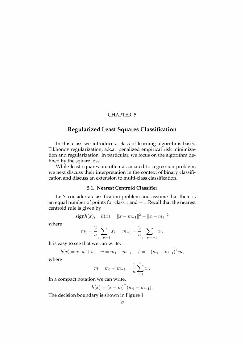
5.1. Nearest Centroid Classifier
Let’s consider a classification problem and assume that there isan equal number of points for class 1 and −1. Recall that the nearestcentroid rule is given by
signh(x), h(x) = ‖x−m−1‖2 − ‖x−m1‖2
wherem1 =
2
n
∑i | yi=1
xi, m−1 =2
n
∑i | yi=−1
xi.
It is easy to see that we can write,
h(x) = x>w + b, w = m1 −m−1, b = −(m1 −m−1)>m,
where
m = m1 +m−1 =1
n
n∑i=1
xi.
In a compact notation we can write,
h(x) = (x−m)>(m1 −m−1).
The decision boundary is shown in Figure 1.17
18 5. REGULARIZED LEAST SQUARES CLASSIFICATION
FIGURE 1. Nearest centroid classifier’s decisionboundary h(x) = 0.
5.2. RLS for Binary Classification
If we consider an offset, the classification rule given by RLS is
signf(x), f(x) = x>w + b,
whereb = −m>w,
since 1n
∑ni=1 yi = 0 by assumption, and
w = (X>nXn + λnI)−1X
>nYn = (
1
nX>nXn + λI)−1 1
nX>nYn,
with Xn the centered data matrix having rows xi −m, i = 1, . . . ,m.It is easy to show a connection between the RLS classification rule
and the nearest centroid rule. Note that,1
nX>NYn =
1
nX>NYn = m1 −m−1,
so that, if we let Cλ = 1nX>nXn + λI
b = −m>C−1λ (m1 −m−1) = −m>w
and
f(x) = (x−m)>C−1λ (m1 −m−1) = x>w + b = (x−m)>w
If λ is large, then ( 1nX>nXn + λI) ∼ λI , and we see that
f(x) ∼ 1
λh(x)⇔ signf(x) = signh(x).
If λ is small Cλ ∼ C = 1nX>nXn, the inner product x>w is replaced
with a new inner product (x − m)>C−1(x − m). The latter is the socalled Mahalanobis distance. If we consider the eigendecomposition
5.3. RLS FOR MULTICLASS CLASSIFICATION 19
of C = V ΣV > we can better understand the effect of the new innerproduct. We have
f(x) = (x−m)>V Σ−1λ−1V >(m1 −m−1) = (x− m)>(m1 − m−1),
where u = Σ1/2V >u. The data are rotated and then stretched in di-rections along which the eigenvalues are small.
5.3. RLS for Multiclass Classification
RLS can be adapted to problems with T > 2 classes by consider-ing
(5.1) (X>nXn + λnI)W = X>n Yn,
where W is a D × T matrix, and Yn is a n × T matrix where the i-th column has entry 1 if the corresponding input belongs to the i-thclass and−1 otherwise. If we letWt, t = 1, . . . , T , denote the columnsof W , then the corresponding classification rule c : X → 1, . . . , Tis
c(x) = arg maxt=1,...,T
x>W t
The above scheme can be seen as a reduction scheme from multiclass to a collection of binary classification problems. Indeed, thesolution of 5.1 can be shown to solve the minimization problem
minW 1,...,WT
T∑t=1
(1
n
n∑i=1
(yti − x>i W t)2 + λ‖W t‖2).
where yti = 1 if xi belongs to class t and yti = −1 otherwise. Theabove minimization can be done separately for all Wi, i = 1, . . . , T .Each minimization problem can be interpreted as performing a ”onevs all” binary classification.


CHAPTER 6
Feature, Kernels and Representer Theorem
In this class we introduce the concepts of feature map and kernel,that allow to generalize Regularization Networks, and not only, wellbeyond linear models. Our starting point will be again Tikhonovregularization,
(6.1) minw∈RD
1
n
n∑i=1
`(yi, fw(xi)) + λ‖w‖2.
6.1. Feature Maps
A feature map is a map
Φ : X → F
from the input space X into a new space F called feature spacewhere there is a scalar product Φ(x)>Φ(x′). The feature space canbe infinite dimensional and the following notation is used for thescalar product 〈Φ(x),Φ(x′)〉F .
6.1.1. Beyond Linear Models. The simplest case is when F =Rp, and we can view the entries Φ(x)j , j = 1, . . . , p as novel mea-surements on the input points. For illustrative purposes, considerX = R2. An example of feature map could be x = (x1, x2) 7→ Φ(x) =
(x21,√
2x1x2, x22). With this choice, if we now consider
fw(x) = w>Φ(x) =
p∑j=1
wjΦ(x)j,
we effectively have that the function is no longer linear but it is apolynomial of degree 2. Clearly the same reasoning holds for muchmore general choices of measurements (features), in fact any finiteset of measurements. Although seemingly simple, the above obser-vation allows to consider very general models. Figure 1 gives a geo-metric interpretation of the potential effect of considering a featuremap. Points which are not easily classified by a linear model, canbe easily classified by a linear model in the feature space. Indeed, themodel is no longer linear in the original input space.
21

22 6. FEATURE, KERNELS AND REPRESENTER THEOREM
FIGURE 1. A pictorial representation of the potentialeffect of considering a feature map in a simple two di-mensional example.
6.1.2. Computations. While feature maps allow to consider non-linear models, the computations are essentially the same as in the lin-ear case. Indeed, it is easy to see that the computations consideredfor linear models, under different loss functions, remain unchanged,as long as we change x ∈ RD into Φ(x) ∈ Rp. For example, for leastsquares we simply need to replace the n × D matrix Xn with a newn×p matrix Φn, where each row is the image of an input point in thefeature space, as defined by the feature map.
6.2. Representer Theorem
In this section we discuss how the above reasoning can be fur-ther generalized. The key result is that the solution of regularizationproblems of the form (6.1) can always be written as
(6.2) w> =n∑i=1
x>i ci,
where x1, . . . , xn are the inputs in the training set and c = (c1, . . . , cn)a set of coefficients. The above result is an instance of the so calledrepresenter theorem. We first discuss this result in the context ofRLS.
6.2.1. Representer Theorem for RLS. The result follows notingthat the following equality holds,
(6.3) (X>nXn + λnI)−1X>n = X>n (XnX>n + λnI)−1,

6.3. KERNELS 23
so that we have,
w = X>n (XnX>n + λnI)−1Yn︸ ︷︷ ︸
c
=n∑i=1
x>i ci.
Equation (6.3) follows from considering the SVD of Xn, that is Xn =UΣV >. Indeed we have X>n = V ΣU> so that
(X>nXn + λnI)−1X>n = V (Σ2 + λ)−1ΣU>
andX>n (XnX
>n + λnI)−1 = V Σ(Σ2 + λ)−1U>.
6.2.2. Representer Theorem Implications. Using Equations 7.2and 6.3, it is possible to show how the vector c of coefficients canbe computed considering different loss functions. In particular, forthe square loss the vector of coefficients satisfies the following linearsystem
(Kn + λnI)c = Yn.
where Kn is the n× n matrix with entries (Kn)i,j = x>i xj . The matrixKn is called the kernel matrix and is symmetric and positive semi-definite.
6.3. Kernels
One of the main advantages of using the representer theorem isthat the solution of the problem depends on the input points onlythrough inner products x>x′. Kernel methods can be seen as replac-ing the inner product with a more general function K(x, x′). In thiscase, the representer theorem 7.2, that is fw(x) = w>x =
∑ni=1 x
>i xci,
becomes
(6.4) f(x) =n∑i=1
K(xi, x)ci.
and we can promptly derive kernelized versions of RegularizationNetworks induced by different loss functions.
The function K is often called a kernel and to be admissible itshould behave like an inner product. More precisely it should be:1) symmetric, and 2) positive definite, that is the kernel matrix Kn
should be positive semi-definite for any set of n input points. Whilethe symmetry property is typically easy to check, positive semi def-initeness is trickier. Popular examples of positive definite kernelsinclude:
• linear kernel K(x, x′) = x>x′,

24 6. FEATURE, KERNELS AND REPRESENTER THEOREM
• polynomial kernel K(x, x′) = (x>x′ + 1)d,
• Gaussian kernel K(x, x′) = e−‖x−x′‖2
2σ2 ,where the last two kernels have a tuning parameter, the degree d andGaussian width σ, respectively.
A positive definite kernel is often called a reproducing kernel andit is a key concept in the theory of reproducing kernel Hilbert spaces.
We end noting that there are some basic operations that can beused to build new kernels. In particular it is easy to see that, ifK1, K2
are reproducing kernels, then K1 +K2 is also a kernel.
CHAPTER 7
Regularization Networks
In this class we introduce a class of learning algorithms based onTikhonov regularization, a.k.a. penalized empirical risk minimiza-tion and regularization. In particular, we study common computa-tional aspects of these algorithms introducing the so called represen-ter theorem.
7.1. Empirical Risk Minimization
Among different approaches to design learning algorithms, em-pirical risk minimization (ERM) is probably the most popular one.The general idea behind this class of methods is to consider the em-pirical error
E(f) =1
n
n∑i=1
`(yi, f(xi)),
as a proxy for the expected error
E(f) = E[`(y, f(x))] =
∫dxdyp(x, y)`(y, f(x)).
Recall that ` is a loss function and measures the price we pay pre-dicting f(x) when in fact the right label is y. Also, recall that theexpected error cannot be directly computed, since the data distribu-tion is fixed but unknown.
In practice, to turn the above idea into an actual algorithm weneed to fix a suitable hypotheses spaceH on which we will minimizeE .
7.2. Hypotheses Space
The hypotheses space should be such that computations are fea-sible and, at the same time, it should be rich, since the complexity ofthe problem is not known a priori. As we have seen, the simplestexample of hypotheses space is the space of linear functions, that is
H = f : RD → R : ∃w ∈ RD such that f(x) = xTw, ∀x ∈ RD.25

26 7. REGULARIZATION NETWORKS
Each function f is defined by a vector w and we let fw(x) = xTw. Wehave also seen how we can vastly extend the class of functions wecan consider by introducing a feature map
Φ : RD → Rp,
where typically p D, and considering functions of the form fw(x) =Φ(x)Tw. We have also seen how this model can be pushed furtherconsidering so called reproducing kernels
K : RD × RD → Rthat are symmetric and positive definite functions, implicitly defin-ing a feature map via the equation
Φ(x)TΦ(x′) = K(x, x′).
If the hypotheses space is rich enough, solely minimizing the em-pirical risk is not enough to ensure a generalizing solution. Indeed,simply solving ERM would lead to estimators which are highly de-pendent on the data and could overfit. Regularization is a generalclass of techniques that allow to restore stability and ensure general-ization.
7.3. Tikhonov Regularization and Representer Theorem
We consider the following Tikhonov regularization scheme,
(7.1) minw∈RD
E(fw) + λ‖w‖2.
The above scheme describes a large class of methods sometimes calledRegularization Networks. The term ‖w‖2 is called regularizer andcontrols the stability of the solution. The parameter λ balances theerror term and the regularizer.
Different classes of methods are induced by the choice of differ-ent loss functions. In the following, we will see common aspects anddifferences in considering different loss functions.
There is no general computational scheme to solve problems ofthe form (7.1), and the actual solution for each algorithm depends onthe considered loss function. However, we show next that for linearfunctions the solution of problem (7.1) can always be written as
(7.2) w = XTn c, f(x) =
n∑i=1
xTxici
where Xn is the n × D data matrix and c = (c1, . . . , cn). This allowson the one hand to reduce computational complexity when n D,or n p in the case of a feature map.

7.4. LOSS FUNCTIONS AND TARGET FUNCTIONS 27
7.3.1. Representer Theorem for General Loss Functions. Herewe discuss the general proof of the representer theorem for loss func-tions other than the square loss.
• The vectors of the form (7.2) form a linear subspace W ofRD. Hence, for every w ∈ RD we have the decompositionw = w + w⊥, where w ∈ W and w⊥ belongs to the space W⊥
of vectors orthogonal to those in W , i.e.
(7.3) wT w⊥ = 0.
• The following is the key observation: for all i = 1, . . . , n xi ∈W , so that
fw(xi) = xTi w = xTi (w + w⊥) = xTi w.
It follows that the empirical error depends only on w!• For the regularizer we have
‖w‖2 = ‖w + w⊥‖2 = ‖w‖2 + ‖w⊥‖2,
because of (7.3). Clearly the above expression is minimizedif we take w⊥ = 0.
The theorem is hence proved, the first term in (7.1) depends only onvector of the form (7.2) and the same form is the best to minimize thesecond term
7.4. Loss Functions and Target Functions
It is useful to recall that different loss functions might define dif-ferent goals via the corresponding target functions.
A simple calculation shows what is the target function corre-sponding to the square loss. Recall that the target function minimizethe expected squared loss error
E(f) =
∫p(x, y)dxdy(y − f(x))2 =
∫p(x)dx
∫p(y|x)dy(y − f(x))2.
To simplify the computation we let
f ∗(x) = arg mina∈R
∫p(y|x)dy(y − a)2,
for all x ∈ X . It is easy to see that the solution is given by
f ∗(x) =
∫dyp(y|x)y
In classification
f ∗(x) = (+1)(p) + (−1)(1− p) = 2p− 1, p = p(1|x), 1− p = p(−1|x)

28 7. REGULARIZATION NETWORKS
which justifies taking the sign of f .Similarly, we can derive the target function of the logistic loss
function,
f ∗(x) = arg mina∈R
∫p(y|x)dy log(1+e−ya) = arg min
a∈Rp log(1+e−a)+(1−p) log(1+ea).
We can simply take the derivative and set it equal to zero,
p−e−a
(1 + e−a)+ (1− p) ea
(1 + ea)= −p 1
(1 + e−a)+ (1− p) ea
(1 + ea)= 0,
so thatp =
ea
(1 + ea)=⇒ a = log
p
1− p

CHAPTER 8
Logistic Regression
We consider logistic regression, that is Tikhonov regularization
(8.1) minw∈RD
E(fw) + λ‖w‖2, E(fw) =1
n
n∑i=1
`(yi, fw(xi))
where the loss function is `(y, fw(x)) = log(1 + e−yfw(x)), namely thelogistic loss function (see Figure 1).
1 2
0.5
1.0
1.5
2.0
0 1 loss
square loss
Hinge loss
Logistic loss
0.5
FIGURE 1. Logistic loss (green) and other loss functions.
Since the logistic loss function is differentiable, the natural can-didate to compute a minimizer is a the gradient descent algorithmwhich we describe next.
8.1. Interlude: Gradient Descent and Stochastic Gradient
Before starting, let’s recall the following basic definition29

30 8. LOGISTIC REGRESSION
• Gradient of G : RD → R,
∇G = (∂G
∂w1, . . . ,
∂G
∂wD)
• Hessian of G : RD → R,
H(G)i,j =∂2G
∂wi∂wj
• Jacobian of F : RD → RD
J(F )i,j =∂F i
∂wj
Note that H(G) = J(∇G).
Consider the minimization problem
minw∈RD
G(w) G : RD → R
when G is a differentiable (strictly convex) function. A general ap-proach to find an approximate solution of the problem is the gradientdescent (GD) algorithm, based on the following iteration
(8.2) wt+1 = wt − γ∇G(wt)
for a suitable initialization w0. Above, ∇G(w) is the gradient of Gat w and γ is a positive constant (or a sequence) called the step-size.Choosing the step-size appropriately ensures the iteration to con-verge to a minimizing solution. In particular, a suitable choice canbe shown to be
γ = 1/L,
where L is the Lipschitz constant of the gradient, that is L such that
‖∇G(w)−∇G(w′)‖ ≤ L‖w − w′‖∀w,w′.
It can be shown that L is less or equal than the biggest eigenvalue ofthe Hessian matrix H(G)(w) for all w. The term descent comes fromthe fact that it can be shown that
G(wt) ≥ G(wt+1)∀wt.
A related technique is called stochastic gradient or also incrementalgradient. To describe this method, we consider an objective functionof the form
G(w) =n∑i=1
gi(w), gi : RD → R, i = 1, . . . , n,

8.2. REGULARIZED LOGISTIC REGRESSION 31
so that ∇G(w) =∑n
i=1∇gi(w). The stochastic gradient algorithmcorresponds to replacing (8.2) with
wt+1 = wt − γ∇git(wt)
where it denotes a deterministic or stochastic sequence of indices. Inthis case, the step size needs to be chosen as sequence γt going tozero but not too fast. For example the choice γt = 1/t can be shownto suffice.
8.2. Regularized Logistic Regression
The corresponding regularized empirical risk minimization prob-lem is called regularized logistic regression. Its solution can be com-puted via gradient descent or stochastic gradient. Note that
∇E(fw) =1
n
n∑i=1
xi−yie−yix
Ti wt−1
1 + e−yixTi wt−1
=1
n
n∑i=1
xi−yi
1 + eyixTi wt−1
so that, for w0 = 0, the gradient descent algorithm applied to (8.1) is
wt = wt−1 − γ
(1
n
n∑i=1
xi−yi
1 + eyixTi wt−1
+ 2λwt−1
)
for t = 1, . . . T , where
1
n
n∑i=1
−yixie−yixTi w
1 + e−yixTi w
+ 2λw = ∇(E(fw) + λ‖w‖2)
A direct computation shows that
J(∇E(fw)) =1
n
n∑i=1
xixTi `′′(yiw
Txi) + 2λI
where `′′(a) = e−a
(1+e−a)2 ≤ 1 is the second derivative of the function`(a) = log(1 + e−a). In particular it can be shown that
L ≤ σmax(1
nXTnXn + 2λI)
where σmax(A) is the largest eigenvalue of a (symmetric positive semi-definite) matrix A.

32 8. LOGISTIC REGRESSION
8.3. Kernel Regularized Logistic Regression
The vector of coefficients can be computed by the following iter-ation
ct = ct−1 − γB(ct−1), t = 1, . . . , T
for c0 = 0, and where B(ct−1) ∈ Rn with
B(ct−1)i = − 1
n
yi
1 + eyi∑nk=1 x
Tk xic
kt−1
+ 2λcit−1.
Here again we choose a constant step-size. Note that
σmax(1
nXTnXn + λI) = σmax(
1
nXnX
Tn + λI) = σmax(
1
nKn + λI).
8.4. Logistic Regression and Confidence Estimation
We end recalling that a main feature of logistic regression is that,as discussed, the solution can be shown to have a probabilistic inter-pretation, in fact it can be derived from the following model
p(1|x) =ex
Tw
1 + exTw,
where the right hand side is called logistic function. This latter ob-servation can be used to compute a confidence on each prediction ofthe logistic regression estimator.

CHAPTER 9
From Perceptron to SVM
We next introduce the support vector machine discussing one ofthe most classical learning algorithms, namely the perceptron algo-rithm.
9.1. Perceptron
The perceptron algorithm finds a linear classification rule accord-ing to the following iterative procedure. Set w0 = 0 and update
wi = wi−1 + γyixi, if yiwTxi ≤ 0
and let wi = wi−1 otherwise. In words, if an example is correctly clas-sified, then the perceptron does not do anything. If the perceptronincorrectly classifies a training example, each of the input weights ismoved a little bit in the correct direction for that training example.The above procedure can be seen as the stochastic (sub) gradient as-sociated to the objective function
n∑i=1
| − yiwTxi|+
where the |a|+ = max0, a. Indeed if yiwTxi < 0, then |−yiwTxi|+ =−yiwTxi and∇|−yiwTxi|+ = −yixi, if yiwTxi > 0, then |−yiwTxi|+ =0 hence∇|− yiwTxi|+ = 0. Clearly, an off-set can also be considered,replacing wTx by wTx+ b and an analogous iteration can be derived.
The above method can be shown to converge for γ = const ifthe data are linearly separable. If the data are not separable, with aconstant step size the perception will typically cycle. Moreover, theperceptron does not implement any specific form of regularizationso in general it is prone to overfitting the data.
9.2. Margin
The quantity α = ywTx defining the objective function of theperceptron is a natural error measure and is sometimes called thefunctional margin. Next we look at a geometric interpretation of thefunctional margin that will lead to a different derivation of Tikhonov
33

34 9. FROM PERCEPTRON TO SVM
regularization for the so called hinge loss function. We begin by con-sidering a binary classification problem where the classes are linearlyseparable.
Consider the decision surface S = x : wTx = 0 defined bya vector w and x such that wTx > 0. It is easy to check that theprojection of x on S is a point xw satisfying
xw = x− β w
‖w‖
where β is the distance between x and S. Clearly, xw ∈ S so that
wT (x− β w
‖w‖) = 0⇔ β =
wT
‖w‖x.
If x is x such that wTx < 0, then β = − wT
‖w‖x so, in general we have
β = ywT
‖w‖x
The above quantity is often called the geometric margin and clearlyif ‖w‖ = 1 it coincides with the geometric margin. Note that themargin is scale invariant, in the sense that β = y w
T
‖w‖x = y 2wT
‖2w‖x, as isthe decision rule sign(wTx).
FIGURE 1. Plot of the margin β between the decisionfunction and the nearest samples.

9.3. MAXIMIZING THE MARGIN 35
9.3. Maximizing the Margin
Maximizing the margin is a natural approach to select a linearseparating rule in the separable case (see Figure 1).
More precisely, consider
βw = mini=1,...,n
βi, βi = yiwT
‖w‖xi, i = 1, . . . , n,
maxw∈RD
βw, subj. to, βw ≥ 0, ‖w‖ = 1.(9.1)
Note that the last constraint is needed to avoid the solution w = ∞(check what happens if you consider a solution w and then scale itby a constant k).
In the following, we manipulate the above expression to obtain aproblem of the form
minw∈RD
F (w), Aw + c ≥ 0,
where F is convex, A is a matrix and c a vector. These are convexprogramming problems which can be efficiently solved.
We begin by rewriting problem (9.1) by introducing a dummyvariable β = βw to obtain
max(w,β)∈RD+1
β, subj. to, yiwT
‖w‖xi ≥ β; β ≥ 0, ‖w‖ = 1
(we are basically using the definition of minimum as the maximumof the infimal points). We next would like to avoid the constraint‖w‖ = 1. It can be shown that the above problem is equivalent toconsidering
max(w,α)∈RD+1
α
‖w‖, subj. to, yiw
Txi ≥ α;α ≥ 0.
with β = α‖w‖ , where the key idea is that the latter problem is scale
invariant. More precisely that we can always restrict ourselves to‖w‖ = 1 by appropriately rescaling the solutions. Using again scaleinvariance (check what happens if you consider a solution w andthen scale it by a constant (kw, kα)), without loss of generality wecan fix α = 1 to obtain
maxw∈RD
1
‖w‖, subj. to, yiw
Txi ≥ 1 , i = 1, . . . , n,
or equivalently
(9.2) minw∈RD
1
2‖w‖2, subj. to, yiw
Txi ≥ 1 , i = 1, . . . , n,

36 9. FROM PERCEPTRON TO SVM
In the above reasoning we assumed data to be separable; if thisis not the case, one could consider slack variables ξ = (ξ1, . . . , ξn) torelax the constraints in the above problem, considering(9.3)
minw∈RD,ξ∈Rn
1
2‖w‖2+C
n∑i=1
, subj. to, yiwTxi ≥ 1−ξi, ξi ≥ 0 , i = 1, . . . , n.
9.4. From Max Margin to Tikhonov Regularization
Note that ξi = max0, 1 − yiwTxi = |1 − yiw
Txi|+, for all i =1, . . . , n. Then if we set λ = 1
2Cn, we have that problem (9.3) is equiv-
alent to
minw∈RD,ξ∈Rn
1
n
n∑i=1
|1− yiwTxi|+ + λ‖w‖2.
9.5. Computations
The derivation of a solution to the SVM problem requires no-tions of convex optimization, specifically considering so called La-grangian duality. Indeed, it can be shown that the solution of prob-lem (9.3) is of the form
w =n∑i=1
yiαixi
where the coefficients αi for i = 1, . . . , n are given by the solution ofthe so called dual problem,(9.4)
minα∈Rn
n∑i=1
αi−1
2
n∑i,j=1
αiαjyiyjxTi xj, subject to 0 ≤ αi ≤ C, i = 1, . . . , n.
where in particular it can be shown that
αi = 0 =⇒ yiwTxi ≥ 1.
9.6. Dealing with an off-set
Finally, it can be shown that the above reasoning can be general-ized to consider an offset, that is wTx + b, in which case we simplyhave to add the constraint
n∑i=1
yiαixi = 0
to the dual problem (9.4).

CHAPTER 10
Dimensionality Reduction
In many practical applications it is of interest to reduce the di-mensionality of the data. In particular, this is useful for data visu-alization, or for investigating the ”effective” dimensionality of thedata. This problem is often referred to as dimensionality reductionand can be seen as the problem of defining a map
M : X = RD → Rk, k D,
according to some suitable criterion.
FIGURE 1. Principal components of a 2D dataset.
37

38 10. DIMENSIONALITY REDUCTION
10.1. PCA & Reconstruction
PCA is arguably the most popular dimensionality reduction pro-cedure. It is a data driven procedure that given an (unsupervised)sample S = (x1, . . . , xn) derives a dimensionality reduction definedby a linear map M . PCA can be derived from several perspectives.Here we provide a geometric/analytical derivation.
We begin by considering the case where k = 1. We are interestedin finding the single most relevant dimension according to somesuitable criterion. Recall that, if w ∈ RD with ‖w‖ = 1, then the (or-thogonal) projection of a point x on w is given by (wTx)w. Considerthe problem of finding the direction p which allows the best possibleaverage reconstruction of the training set, that is the solution of theproblem
(10.1) minw∈SD−1
1
n
n∑i=1
‖xi − (wTxi)w‖2,
where SD−1 = w ∈ RD | ‖w‖ = 1 is the sphere in D dimensions.The norm ‖xi − (wTxi)w‖2 measures how much we lose by project-ing x along the direction w, and the solution p to problem (10.1) iscalled the first principal component of the data. A direct compu-tation shows that ‖xi − (wTxi)w‖2 = ‖xi‖ − (wTxi)
2, so that prob-lem (10.1) is equivalent to
(10.2) maxw∈SD−1
1
n
n∑i=1
(wTxi)2.
This latter observation is useful for two different reasons that the wediscuss in the following.
10.2. PCA and Maximum Variance
If the data are centered, that is x = 1nxi = 0, problem (10.2) has
the following interpretation: we look for the direction along whichthe data have (on average) maximum variance. Indeed, we can in-terpret the term (wTx)2 as the variance of x in the direction w. If thedata are not centered, to keep this interpretation we should replaceproblem (10.2) with
(10.3) maxw∈SD−1
1
n
n∑i=1
(wT (xi − x))2,

10.4. BEYOND THE FIRST PRINCIPAL COMPONENT 39
which corresponds to the original problem on the centered data xc =x − x. In the terms of problem (10.1), it is easy to see that this corre-sponds to considering
(10.4) minw,b∈SD−1
1
n
n∑i=1
‖xi − ((wT (xi − b))w + b)‖2.
where ((wT (xi − b))w + b is an affine transformation (rather than anorthogonal projection).
10.3. PCA and Associated Eigenproblem
A simple further manipulation allows to write problem (10.2) asan eigenvalue problem. Indeed, using the symmetry of the innerproduct we have
1
n
n∑i=1
(wTxi)2 =
1
n
n∑i=1
wTxiwTxi =
1
n
n∑i=1
wTxixTi w = wT (
1
n
n∑i=1
xixTi )w
so that problem (10.2) can be written as
(10.5) maxw∈SD−1
wTCnw, Cn =1
n
n∑i=1
xixTi .
We need two observations. First, in matrix notation Cn = XTnXn and
it is easy to see that Cn is symmetric and positive semi-definite. If thedata are centered, the matrix Cn is the so called covariance matrix.Clearly, the objective function in (10.5) can be written as
wTCnw
wTwwhere the latter quantity is the so called Rayleigh quotient. Notethat, if Cnu = λu then uTCnu
uTu= λ, since the eigenvector u is nor-
malized. In fact, it is possible to show that the Rayleigh quotientachieves its maximum at a vector which corresponds to the maxi-mum eigenvalue of Cn (the proof of this latter fact uses basic resultsin linear programming). Then, computing the first principal compo-nent of the data is reduced to computing the biggest eigenvalue ofthe covariance and the corresponding eigenvector.
10.4. Beyond the First Principal Component
Next, we discuss how the above reasoning can be generalized tok > 1, that is more than one principle component. The idea is simplyto iterate the above reasoning to describe the input data beyond whatis allowed by the first principal component. Towards this end, we

40 10. DIMENSIONALITY REDUCTION
consider the one-dimensional projection which can best reconstructthe residuals
ri = xi − (pTxi)pi,
that is we replace problem (10.1) by
(10.6) minw∈SD−1,w⊥p
1
n
n∑i=1
‖ri − (wT ri)w‖2.
Note that for all i = 1, . . . , n,
‖ri − (wT ri)w‖2 = ‖ri‖2 − (wT ri)2 = ‖ri‖2 − (wTxi)
2
since w ⊥ p. Then, following the reasoning from (10.1) to (10.2),problem (10.6) can equivalently be written as
(10.7) maxw∈SD−1,w⊥p
1
n
n∑i=1
(wTxi)2 = wTCnw.
Again, we have to minimize the Rayleigh quotient of the covariancematrix. However, when compared to (10.2), we see that there is thenew constraint w ⊥ p. Indeed, it can be proven that the solutionof problem (10.7) is given by the second eigenvector of Cn, and thecorresponding eigenvalue. The proof of this latter fact follows thesame line of the one for the first principal component. Clearly, theabove reasoning can be generalized to consider more than two com-ponents. The computation of the principal components reduces tothe problem of finding the eigenvalues and eigenvectors of Cn. Thecomplexity of this problem is roughly O(kD2), being k the numberof components (note that the complexity of forming Cn is O(nD2)).
The principal components can be stacked as rows of a k ×D ma-trix M , and in fact, because of the orthogonality constraint, the ma-trix M is orthogonal, MMT = I . The dimensionality reduction in-duced by PCA is hence linear.
10.5. Singular Value Decomposition
We recall the notion of singular value decomposition of a matrixwhich allows in some situations to improve the computations of theprincipal components, while suggesting a possible way to generalizethe algorithm to consider non linear dimensionality reduction.
Considering the data matrixXn, its singular value decompositionis given by
Xn = UΣP T .
where U is a n × d orthogonal matrix, P is a D × d orthogonal ma-trix, Σ is a diagonal matrix such that Σi,i =
√λi, i = 1, . . . , d and

10.6. KERNEL PCA 41
d ≤ minn,D. The columns of U and the columns of V are called re-spectively the left and right singular vectors and the diagonal entriesof Σ the singular values. The singular value decomposition can beequivalently described by the following equations, for j = 1, . . . , d,
Cnpj = λjpj,1
nKnuj = λjuj,
Xnpj =√λjuj,
1
nXTn uj =
√λjpj,(10.8)
where Cn = 1nXTnXn and 1
nKn = 1
nXnX
Tn .
If n p the above equations can be used to speed up the com-putation of the principal components. Indeed, we can consider thefollowing procedure:
(1) form the matrix Kn, which is O(Dn2),(2) find the first k eigenvectors of Kn, which is O(kn2),(3) find the principal components using (10.8), i.e.
(10.9) pj =1√λjXTn uj =
1√λj
n∑i=1
xiuij, j = 1, . . . , d
where u = (u1, . . . , un), which is again O(knd) if we considerk principal components.
10.6. Kernel PCA
The latter reasoning suggests how to generalize the intuition be-hind PCA beyond linear dimensionality reduction by using kernels(or feature maps). Indeed, from equation (10.9) we can see that theprojection of a point x on a principal component p can be written as
(10.10) (M(x))j = xTpj =1√λjxTXT
n uj =1√λj
n∑i=1
xTxiuij,
for j = 1, . . . , d.What if we were to map the data using a possibly non linear fea-
ture map Φ : X → F , before performing PCA? If the feature map isfinite dimensional, e.g. F = Rp we could simply replace x 7→ Φ(x)and follow exactly the same reasoning as in the previous sections.Note in particular that equation (10.10) becomes
(10.11) (M(x))j = Φ(x)Tpj =1√λj
n∑i=1
Φ(x)TΦ(xi)uij,

42 10. DIMENSIONALITY REDUCTION
for j = 1, . . . , d. More generally, one could consider a positive defi-nite kernel K : X ×X → R, in which case (10.10) becomes
(10.12) (M(x))j =1√λj
n∑i=1
K(x, xi)uij,
for j = 1, . . . , d. Note that in this latter case, while it is not clear howto form Cn, we can still form and diagonalize Kn, which is in fact thekernel matrix.

CHAPTER 11
Variable Selection
In many practical situations, beyond predictions it is importantto obtain interpretable results. Interpretability is often related to de-tecting which factors have determined our prediction. We look atthis question from the perspective of variable selection.
Consider a linear model
(11.1) fw(x) = wTx =v∑i=1
wjxj.
Here we can think of the components xjof an input as of specificmeasurements: pixel values in the case of images, dictionary wordcounting in the case of texts, etc. Given a training set, the goal ofvariable selection is to detect which variables are important for pre-diction. The key assumption is that the best possible prediction ruleis sparse, that is only few of the coefficients in (11.1) are differentfrom zero.
11.1. Subset Selection
A brute force approach would be to consider all the training setsobtained considering all the possible subsets of variables. More pre-cisely we could begin by considering only the training set where weretain the first variable of each input points. Then the one where weretain only the second, and so on and so forth. Next, we could passto consider a training set with pairs of variables, then triplets etc. Foreach training set one would solve the learning problem and eventu-ally end selecting the variables for which the corresponding trainingset achieves the best performance.
The described approach has an exponential complexity and be-comes unfeasible already for relatively small D. If we consider thesquare loss, it can be shown that the corresponding problem couldbe written as
(11.2) minw∈RD
1
n
n∑i=1
(yi − fw(xi))2 + λ‖w‖0,
43

44 11. VARIABLE SELECTION
where‖w‖0 = |j | wj 6= 0|
is called the `0 norm and counts the number of non zero componentsin w. In the following we focus on the least squares loss and con-sider different approaches to find approximate solution to the aboveproblem, namely greedy methods and convex relaxation.
11.2. Greedy Methods: (Orthogonal) Matching Pursuit
Greedy approaches are often considered to find approximate so-lutions to problem (11.2). This class of approaches to variable selec-tion generally encompasses the following steps:
(1) initialize the residual, the coefficient vector, and the indexset,
(2) find the variable most correlated with the residual,(3) update the index set to include the index of such variable,(4) update/compute coefficient vector,(5) update residual.
The simplest such procedure is called forward stage-wise regressionin statistics and matching pursuit (MP) in signal processing. To de-scribe the procedure we need some notation. Let Xn be the n × Ddata matrix and Xj ∈ Rn, j = 1, . . . , D be the columns of Xn. LetYn ∈ Rn be the output vector. Let r, w, I denote the residual, thecoefficient vector, an index set, respectively.
The MP algorithm starts by initializing the residual r ∈ Rn, thecoefficient vector w ∈ RD, and the index set I ⊆ 1, . . . , D,
r0 = Yn, , w0 = 0, I0 = ∅.The following procedure is then iterated for i = 1, . . . , T − 1. Thevariable most correlated with the residual is given by
k = arg maxj=1,...,D
aj, aj =(rTi−1X
j)2
‖Xj‖2,
where we note that
vj =rTi−1X
j
‖Xj‖2= arg min
v∈R‖ri−1−Xjv‖2, ‖ri−1−Xjvj‖2 = ‖ri−1‖2− aj
The selection rule has then two interpretations. We select the vari-able such that the projection of the output on the corresponding col-umn is larger, or, equivalently, we select the variable such that thecorresponding column best explains the the output vector in a leastsquares sense.

11.3. CONVEX RELAXATION: LASSO & ELASTIC NET 45
Then, the index set is updated as Ii = Ii−1 ∪ k, and the coeffi-cients vector is given by
(11.3) wi = wi−1 + wk, wkk = vkek
where ek is the element of the canonical basis in RD, with k-th com-ponent different from zero. Finally, the residual is updated
ri = ri−1 −Xwk.A variant of the above procedure, called Orthogonal Matching Pur-suit, is also often considered. The corresponding iteration is analo-gous to that of MP, but the coefficient computation (11.3) is replacedby
wi = arg minw∈RD
‖Yn −XnMIiw‖2,
where the D × D matrix MI is such that (MIw)j = wj if j ∈ I and(MIw)j = 0 otherwise. Moreover, the residual update is replaced by
ri = Yn −Xnwi.
11.3. Convex Relaxation: LASSO & Elastic Net
Another popular approach to find an approximate solution toproblem (11.2) is based on a convex relaxation. Namely, the `0 normis replaced by the `1 norm,
‖w‖1 =D∑j=1
|wj|,
so that, in the case of least squares, problem (11.2) is replaced by
(11.4) minw∈RD
1
n
n∑i=1
(yi − fw(xi))2 + λ‖w‖1.
The above problem is called LASSO in statistics and Basis Pursuit insignal processing. The objective function defining the correspondingminimization problem is convex but not differentiable. Tools fromnon-smooth convex optimization are needed to find a solution. Asimple yet powerful procedure to compute a solution is based onthe so called Iterative Soft Thresholding Algorithm (ISTA). The latteris an iterative procedure where, at each iteration, a non linear softthresholding operator is applied to a gradient step. More precisely,ISTA is defined by the following iteration
w0 = 0, wi = Sλγ(wi−1 −2γ
nXTn (Yn −Xnwi−1)), i = 1, . . . , Tmax

46 11. VARIABLE SELECTION
which should be run until a convergence criterion is met, e.g. ‖wi −wi−1‖ ≤ ε, for some precision ε, or a prescribed maximum number ofiterations Tmax is reached. To ensure convergence we should choosethe step-size γ = n
2‖XTnXn‖
.Note that the argument of the soft thresholding operator corre-
sponds to a step of gradient descent. Indeed,
2
nXTn (Yn −Xnwi−1)
The soft thresholding operator acts component-wise on a vector w,so that
Sα(u) = ||u| − α|+u
|u|.
A depiction of the sof thresholding is shown in Figure 1.The above expression shows that the coefficients of the solution
of problem (11.2) as computed by ISTA can be exactly zero: this canbe contrasted with Tikhonov regularization where this is hardly thecase.
Indeed, it is possible to see that, on the one hand, while Tikhonovallows to compute a stable solution, in general its solution is notsparse. On the other hand, the solution of LASSO might not be sta-ble. The elastic net algorithm, defined as
(11.5) minw∈RD
1
n
n∑i=1
(yi−fw(xi))2+λ(α‖w‖1+(1−α)‖w‖2
2), α ∈ [0, 1],
can be seen as hybrid algorithm which is interpolated between Tikhonovand LASSO. The ISTA procedure can be adapted to solve the elastic
FIGURE 1. The 1-dimensional soft thresholding opera-tor Sλ with threshold λ.

11.3. CONVEX RELAXATION: LASSO & ELASTIC NET 47
net problem, where the gradient descent step incorporates also thederivative of the `2 penalty term. The resulting algorithm is
w0 = 0, wi = Sλαγ((1−λγ(1−α))wi−1−2γ
nXTn (Yn−Xnwi−1)), i = 1, . . . , Tmax
To ensure convergence, we should choose the step-size γ = n2(‖XT
nXn‖+λ(1−α)).


CHAPTER 12
A Glimpse Beyond The Fence
We next try to give a brief overview of 1) topics in machine learn-ing that we have not touched upon, 2) some of the current and futurechallenges in machine learning.
12.1. Different Kinds of Data
Different machine learning approaches arise to deal with differ-ent kinds of input and output. Recall that the input/output pairs areassumed to belong to an input space X and an output space Y , re-spectively. We call Z = X×Y the data space. We list a few examplesof input and output spaces.
• Euclidean/Vector Spaces. Perhaps the simples example, cov-ering many practical situations, is X = Rd, d ∈ N.• Probability distributions. We could setX = x ∈ Rd
+ :∑d
j=1 xj =
1, d ∈ N, and view elements of the space as probability dis-tributions on a finite set Ω of dimension d. More generallygiven any probability space Ω we can view X as the space ofprobability distribution on Ω.• Strings/Words. Given an alphabet Σ of symbols (letters),
one could consider X = Σp, p ∈ N, the (finite) space ofstrings (words) of p letters.• Graphs. We can view X as collection of graphs, i.e. X = .
Clearly more exotic examples can be constructed considering com-positions of the above examples, for example X = Rd × Σp, d, p ∈ Netc.
Next, we discuss different choices of the output space and seehow they often correspond to problems with different names.
• Regression, Y = R.• Binary classification, Y = −1, 1. Where we note that here
we could have taken Y = 0, 1– as well as any other pair ofdistinct numeric values.• Multivariate regression, Y = RT , T ∈ N, each output is a
vector.49

50 12. A GLIMPSE BEYOND THE FENCE
• Functional regression, Y is a Hilbert space, for example eachoutput is a function.• Multi-category classification, Y = 1, 2, . . . , T, T ∈ N, the
output is one of T categories.• Multilabel, Y = 21,2,...,T, T ∈ N, each output is any subset
of T categories.
An interesting case is that of so called multitask learning. HereZ = (X1, Y1) × (X2, Y2) × · · · × (XT , YT )) and the training set is isS = (S1, S2, . . . , ST ). We can view each data space/training set ascorresponding to different, yet related, tasks. In full generality, in-put/output spaces and data cardinality can be different.
12.2. Data and Sampling Models
The standard data model we consider is a training set as an i.i.d.sample from a distribution p on the data space Z.
• Semisupervised, the more general situation where unlabelleddata Su are available together with the labelled data S.• Transductive, related to the above setting, unlabelled dataSu are available together with the labelled data and the goalis to predict the label of the unlabeled data set Su.• Online/Dynamic Learning, the data are not i.i.d. The sam-
ples can be dependent, can come from varying distribution,or both.
12.3. Learning Approaches
• Online/Incremental• Randomized• Distributed• Online/Dynamic Learning, the data are not i.i.d. The sam-
ples can be dependent, the samples can come from varyingdistribution or both.
• Active• Reinforcement Learning
12.4. Some Current and Future Challenges in Machine Learning
Challenges
1← Data Size→∞
12.4. SOME CURRENT AND FUTURE CHALLENGES IN MACHINE LEARNING 51
12.4.1. Big Data? Recent times have seen the development oftechnologies for gathering data-set of unprecedented size and com-plexity both in natural science and technology. On the one handthis has opened novel opportunities (e.g. online teaching), on theother had it has posed new challenges. In particular, the necessityhas emerged to develop learning techniques capable to leverage pre-defined budgets and requisites in terms of
• Computations,• Communications,• Privacy.
12.4.2. Or Small Data? One of the most evident differences be-tween biological and artificial intelligence is the astounding ability ofhumans to generalize from limited supervised data. Indeed, whileimpressive, current artificial intelligent systems based on supervisedlearning require huge amounts of humanly annotated data.
• Unsupervised learning of data representation• Learning under weak supervision.• Learning and exploiting structure among learning tasks.


APPENDIX A
Mathematical Tools
These notes present a brief summary of some of the basic defini-tions from calculus that we will need in this class. Throughout thesenotes, we assume that we are working with the base field R.
A.1. Structures on Vector Spaces
A vector space V is a set with a linear structure. This means wecan add elements of the vector space or multiply elements by scalars(real numbers) to obtain another element. A familiar example of avector space is Rn. Given x = (x1, . . . , xn) and y = (y1, . . . , yn) inRn, we can form a new vector x + y = (x1 + y1, . . . , xn + yn) ∈ Rn.Similarly, given r ∈ R, we can form rx = (rx1, . . . , rxn) ∈ Rn.
Every vector space has a basis. A subset B = v1, . . . , vn of Vis called a basis if every vector v ∈ V can be expressed uniquelyas a linear combination v = c1v1 + · · · + cmvm for some constantsc1, . . . , cm ∈ R. The cardinality (number of elements) of V is calledthe dimension of V . This notion of dimension is well defined be-cause while there is no canonical way to choose a basis, all bases ofV have the same cardinality. For example, the standard basis on Rn
is e1 = (1, 0, . . . , 0), e2 = (0, 1, 0, . . . , 0), . . . , en = (0, . . . , 0, 1). Thisshows that Rn is an n-dimensional vector space, in accordance withthe notation. In this section we will be working with finite dimen-sional vector spaces only.
We note that any two finite dimensional vector spaces over R areisomorphic, since a bijection between the bases can be extended lin-early to be an isomorphism between the two vector spaces. Hence,up to isomorphism, for every n ∈ N there is only one n-dimensionalvector space, which is Rn. However, vector spaces can also haveextra structures that distinguish them from each other, as we shallexplore now.
A distance (metric) on V is a function d : V × V → R satisfying:• (positivity) d(v, w) ≥ 0 for all v, w ∈ V , and d(v, w) = 0 if
and only if v = w.• (symmetry) d(v, w) = d(w, v) for all v, w ∈ V .
53

54 A. MATHEMATICAL TOOLS
• (triangle inequality) d(v, w) ≤ d(v, x)+d(x,w) for all v, w, x ∈V .
The standard distance function on Rn is given by d(x, y) =√
(x1 − y1)2 + · · ·+ (xn − yn)2.Note that the notion of metric does not require a linear structure, orany other structure, on V ; a metric can be defined on any set.
A similar concept that requires a linear structure on V is norm,which measures the “length” of vectors in V . Formally, a norm is afunction ‖ · ‖ : V → R that satisfies the following three properties:
• (positivity) ‖v‖ ≥ 0 for all v ∈ V , and ‖v‖ = 0 if and only ifv = 0.• (homogeneity) ‖rv‖ = |r|‖v‖ for all r ∈ R and v ∈ V .• (subadditivity) ‖v + w‖ ≤ ‖v‖+ ‖w‖ for all v, w ∈ V .
For example, the standard norm on Rn is ‖x‖2 =√x2
1 + · · ·+ x2n,
which is also called the `2-norm. Also of interest is the `1-norm‖x‖1 = |x1| + · · · + |xn|, which we will study later in this class inrelation to sparsity-based algorithms. We can also generalize theseexamples to any p ≥ 1 to obtain the `p-norm, but we will not do thathere.
Given a normed vector space (V, ‖ ·‖), we can define the distance(metric) function on V to be d(v, w) = ‖v − w‖. For example, the`2-norm on Rn gives the standard distance function
d(x, y) = ‖x− y‖2 =√
(x1 − y1)2 + · · ·+ (xn − yn)2,
while the `1-norm on Rn gives the Manhattan/taxicab distance,
d(x, y) = ‖x− y‖1 = |x1 − y1|+ · · ·+ |xn − yn|.As a side remark, we note that all norms on a finite dimensional
vector space V are equivalent. This means that for any two norms µand ν on V , there exist positive constants C1 and C2 such that for allv ∈ V , C1µ(v) ≤ ν(v) ≤ C2µ(v). In particular, continuity or conver-gence with respect to one norm implies continuity or convergencewith respect to any other norms in a finite dimensional vector space.For example, on Rn we have the inequality ‖x‖1/
√n ≤ ‖x‖2 ≤ ‖x‖1.
Another structure that we can introduce to a vector space is theinner product. An inner product on V is a function 〈·, ·〉 : V ×V → Rthat satisfies the following properties:
• (symmetry) 〈v, w〉 = 〈w, v〉 for all v, w ∈ V .• (linearity) 〈r1v1+r2v2, w〉 = r1〈v1, w〉+r2〈v2, w〉 for all r1, r2 ∈R and v1, v2, w ∈ V .• (positive-definiteness) 〈v, v〉 ≥ 0 for all v ∈ V , and 〈v, v〉 = 0
if and only if v = 0.

A.1. STRUCTURES ON VECTOR SPACES 55
For example, the standard inner product on Rn is 〈x, y〉 = x1y1 + · · ·+xnyn, which is also known as the dot product, written x · y.
Given an inner product space (V, 〈·, ·〉), we can define the normof v ∈ V to be ‖v‖ =
√〈v, v〉. It is easy to check that this definition
satisfies the axioms for a norm listed above. On the other hand, notevery norm arises from an inner product. The necessary and suffi-cient condition that has to be satisfied for a norm to be induced byan inner product is the paralellogram law:
‖v + w‖2 + ‖v − w‖2 = 2‖v‖2 + 2‖w‖2.
If the parallelogram law is satisfied, then the inner product can bedefined by polarization identity:
〈v, w〉 =1
4
(‖v + w‖2 − ‖v − w‖2
).
For example, you can check that the `2-norm on Rn is induced bythe standard inner product, while the `1-norm is not induced by aninner product since it does not satisfy the parallelogram law.
A very important result involving inner product is the followingCauchy-Schwarz inequality:
〈v, w〉 ≤ ‖v‖‖w‖ for all v, w ∈ V.Inner product also allows us to talk about orthogonality. Two
vectors v and w in V are said to be orthogonal if 〈v, w〉 = 0. In par-ticular, an orthonormal basis is a basis v1, . . . , vn that is orthogonal(〈vi, vj〉 = 0 for i 6= j) and normalized (〈vi, vi〉 = 1). Given an or-thonormal basis v1, . . . , vn, the decomposition of v ∈ V in terms ofthis basis has the special form
v =n∑i=1
〈v, vn〉vn.
For example, the standard basis vectors e1, . . . , en form an orthonor-mal basis of Rn. In general, a basis v1, . . . , vn can be orthonormalizedusing the Gram-Schmidt process.
Given a subspace W of an inner product space V , we can definethe orthogonal complement ofW to be the set of all vectors in V thatare orthogonal to W ,
W⊥ = v ∈ V | 〈v, w〉 = 0 for all w ∈ W.If V is finite dimensional, then we have the orthogonal decompo-sition V = W ⊕ W⊥. This means every vector v ∈ V can be de-composed uniquely into v = w + w′, where w ∈ W and w′ ∈ W⊥.
56 A. MATHEMATICAL TOOLS
The vector w is called the projection of v on W , and represents theunique vector in W that is closest to v.
A.2. Matrices
In addition to talking about vector spaces, we can also talk aboutoperators on those spaces. A linear operator is a function L : V → Wbetween two vector spaces that preserves the linear structure. In fi-nite dimension, every linear operator can be represented by a matrixby choosing a basis in both the domain and the range, i.e. by workingin coordinates. For this reason we focus the first part of our discus-sion on matrices.
If V is n-dimensional and W is m-dimensional, then a linear mapL : V → W is represented by an m × n matrix A whose columnsare the values of L applied to the basis of V . The rank of A is thedimension of the image of A, and the nullity of A is the dimensionof the kernel of A. The rank-nullity theorem states that rank(A) +nullity(A) = m, the dimension of the domain of A. Also note thatthe transpose of A is an n×m matrix A> satisfying
〈Av,w〉Rm = (Av)>w = v>A>w = 〈v, A>w〉Rn
for all v ∈ Rn and w ∈ Rm.Let A be an n × n matrix with real entries. Recall that an eigen-
value λ ∈ R of A is a solution to the equation Av = λv for somenonzero vector v ∈ Rn, and v is the eigenvector of A correspondingto λ. If A is symmetric, i.e. A> = A, then the eigenvalues of A arereal. Moreover, in this case the spectral theorem tells us that there isan orthonormal basis of Rn consisting of the eigenvectors of A. Letv1, . . . , vn be this orthonormal basis of eigenvectors, and let λ1, . . . , λnbe the corresponding eigenvalues. Then we can write
A =n∑i=1
λiviv>i ,
which is called the eigendecomposition of A. We can also write thisas
A = V ΛV >,
where V is the n×n matrix with columns vi, and Λ is the n×n diag-onal matrix with entries λi. The orthonormality of v1, . . . , vn makesV an orthogonal matrix, i.e. V −1 = V >.
A symmetric n×nmatrixA is positive definite if v>Av > 0 for allnonzero vectors v ∈ Rn. A is positive semidefinite if the inequality

A.2. MATRICES 57
is not strict (i.e.≥ 0). A positive definite (resp. positive semidefinite)matrix A has positive (resp. nonnegative) eigenvalues.
Another method for decomposing a matrix is the singular valuedecomposition (SVD). Given an m × n real matrix A, the SVD of Ais the factorization
A = UΣV >,
where U is an m × m orthogonal matrix (U>U = I), Σ is an m × ndiagonal matrix, and V is an n × n orthogonal matrix (V >V = I).The columns u1, . . . , um of U form an orthonormal basis of Rm, andthe columns v1, . . . , vn of V form an orthonormal basis of Rn. Thediagonal elements σ1, . . . , σminm,n in Σ are nonnegative and calledthe singular values of A. This factorization corresponds to the de-composition
A =
minm,n∑i=1
σiuiv>i .
This decomposition shows the relations between σi, ui, and vi moreclearly: for 1 ≤ i ≤ minm,n,
Avi = σiui AA>ui = σ2i ui
A>ui = σivi A>Avi = σ2i vi
This means the ui’s are eigenvectors ofAA>with corresponding eigen-values σ2
i , and the vi’s are eigenvectors ofA>A, also with correspond-ing eigenvalues σ2
i .Given an m × n matrix A, we can define the spectral norm of A
to be largest singular value of A,
‖A‖spec = σmax(A) =√λmax(AA>) =
√λmax(A>A).
Another common norm on A is the Frobenius norm,
‖A‖F =
√√√√ m∑i=1
n∑j=1
a2ij =
√trace(AA>) =
√trace(A>A) =
√√√√minm,n∑i=1
σ2i .
However, since the space of all matrices can be identified with Rm×n,the discussion in Section A.1 still holds and all norms onA are equiv-alent.