Embed Size (px)
Citation preview

Introductory LATEX
Dr N.L.C. Talbot
for
UEA Centre for Staff and Educational Development
Introductory LATEX 1

Course Summary
• Getting Started
– Basic text, punctuation, accents and symbols.
– Simple font changing commands.
– Document styles, sectioning commands, and title pages.
– Paragraph justification.
– Defining new commands.
– Converting to PostScript
• Basic Formatting
– Lists and tabulated material.
• Basic mathematics.
Introductory LATEX 2

Course Summary Continued
• Cross-referencing
• Packages
• Citations
• Lengths
• Boxes and minipages
• Incorporating PostScript pictures
• Figures and tables
• Creating slides
• Defining new environments
• Counters
Introductory LATEX 3

Course Materials
• Each participant should have been given a handout.
• In addition, the following material is available on the web:
– PostScript versions of the handouts and slides
– LaTeX source code for the handouts and slides
– On-line version of the slides
– Advice and solutions to the exercises
– Terminology so that you can check the definition of a keyword.
These can be found at:http://theoval.sys.uea.ac.uk/~gcc/family/nicky/csed.html
Introductory LATEX 4

Some Notes
• At the end of each topic there will be an exercise for you to do togive you some practical experience with the topic.
• Be sure to read the instructions given in the handout, and payparticular attention to any Notes.
• Advice and explanations to common errors are available on-line.
• LATEX and UNIX are both case-sensitive, so be sure to typecommands exactly as they appear in the handout.
• A triangle I indicates something to be typed in at the UNIXcommand prompt. For example:Ilatex filename
(Remember to press the return key at the end of the line.)
Introductory LATEX 5

Logging On
• We will be using eXceed.
• eXceed allows us to access CPC’s UNIX computers fromWindows NT.
• You should all have a username and password for this course.
• To run eXceed, double-click on the icon Staff1.
Introductory LATEX 6

Using UNIX
• UNIX is command line driven.
• Commands are typed in at the command prompt.
• Some simple commands:
ls lists the contents of the current directory.
mkdir makes a new directory. e.g.Imkdir latex
will create a directory called latex.
cd change directory. e.g.Icd latex
will change to the directory called latex.
cp copies a file to a new location. We will be using thiscommand in some of the exercises.
Introductory LATEX 7

Initialising Your Account
• If you want to use dxnotepad, you will have to fix a bug in thekey findings. To do this type:
Icd
I/sw1/bin/dxnotepadfix
• To initialise your account so that you can use LATEX, you musttype the following commands at the command prompt:
Icd .uea-options
Itouch tex
Ilogout
This will exit eXceed, so you will now have to run eXceed again.
Once you have done this, you don’t need to do it again next time youlogon.
Introductory LATEX 8

What is TEX/LATEX?
• TEX is a typesetting language written by Donald Knuth.
• Original format of TEX called: “plain TEX”.
• Plain TEX is not very easy to use.
• Leslie Lamport wrote a format of TEX called LATEX.
• LATEX much easier to use.
• Since LATEX is a format of TEX, some of the errors you mayencounter will be TEX errors, and some errors will be LATEXerrors.
• We will be using LATEX2e version.
Introductory LATEX 9

Getting Started
• Unlike a word processor, you must first write the source code in afile (input file) which is then converted into typeset output.
• LATEX source code is written in a file with extension .tex usingan ordinary text editor.
• Any standard keyboard character may be used, but there are 10special characters:
# $ % & { } _ ~ \ ^
These characters only occur in LATEX commands.
• To produce the first seven of the above characters, you mustprecede it with a backslash, for example, \$ will print a dollarsign.
Introductory LATEX 10

Commands (Macros)
• Commands are available to specify how to format parts of thedocument. For example, \twocolumn will start a new page andchange the document to two column layout.
• Almost all LATEX commands start with a backslash, e.g. \today,which prints the current date.
• Any spaces following a command are ignored. For example:
\TeX pert
Input
TEXpert
Output
Note that \TeXpert will give an error.
Introductory LATEX 11

Grouping
• Segments of code may be grouped by placing it within { and }• Most commands occurring within a group will be local to that
group.
Some text. {This text
is \em within a group.}
Some more text.
Input
Some text. This textis within a group.Some more text.
Output
• A command may be grouped to avoid placing a space after it:
{\TeX}pert
Input
TEXpert
Output
Introductory LATEX 12

Command Arguments
• Some commands take one or more arguments. For example, thecommand \textbf takes one argument, and will typeset thatargument in a bold font.
\textbf{Some bold text}
Input
Some bold text
Output
• Note that if the argument consists of more that one character, itmust be grouped using braces { }, if not, only the first object willbe taken as the argument:
\textbf Some bold text
Input
Some bold text
Output
Introductory LATEX 13

Optional Arguments
• Some commands have optional arguments.
• Optional arguments are always enclosed in square brackets [ ]:
A new\\
line.
Input
A newline.
Output
A new\\[10pt]
line.
Input
A new
line.
Output
• Optional arguments almost always come before mandatoryarguments (although there are a few exceptions.)
Introductory LATEX 14

Environments
• An environment is different to a command.
• \begin{〈name〉} indicates the beginning of an environment.
• \end{〈name〉} indicates the end of an environment.
• \begin{sffamily}
Some sans-serif text.
\end{sffamily}
Input
Some sans-serif text.
Output
• Environments form implicit grouping. Changes made within anenvironment are usually local.
• Environments may also have optional or mandatory arguments.
Introductory LATEX 15

Spaces
• Consecutive spaces are treated as one single space.
Some text.
Input
Some text.
Output
• Newline characters are treated as a space.• To force a space after a command, use \Ã:
\LaTeX\ is great!
Input
LATEX is great!
Output
• Also use \Ã after lowercase abbreviations:
e.g.\ like this.
Input
e.g. like this.
Output
Introductory LATEX 16

Paragraphs
• Completely blank lines indicate the end of a paragraph.
Here is the first
paragraph.
This is the start
of the second
paragraph.
Input
Here is the firstparagraph.This is the start
of the second para-graph.
Output
• A paragraph break can also be specified by the command \par
Introductory LATEX 17

Creating a Document
• At the start of any LATEX2e file, you must have the command\documentclass, which declares what class to use. For example:
\documentclass[a4paper,12pt]{article}
• All the text that is actually contained in the document must beenclosed between the commands:
\begin{document}
which specifies the start of the document, and
\end{document}
which specifies the end of the document.
Introductory LATEX 18

Exercise 1 : Creating a Simple Document
(See Page 1)
• Open dxnotepad, and type in the contents of Figure 1 on page 2of the handouts.
• Save your file as exercise1.tex.
• Go to the command window, and type:Ilatex exercise1
• If there were no errors, you should now have three extra files:exercise1.aux, exercise1.log and exercise1.dvi.
• To view the typeset document, type the following at thecommand prompt:
Ixdvi exercise1.dvi
Introductory LATEX 19

Font Changing Commands
verses
Font Changing Declarations
A Font Changing Command is something that does not affectthe rest of the document. It effectively says: do this to thefollowing object. For example, \textbf{A} says: “make thefollowing object bold”, where the following object is the letter‘A’.
A Font Changing Declaration is something that affects thedocument from that point onwards. For example, \bfseries willswitch to a bold font from the point where it is declared, onwards.
Introductory LATEX 20

Font Changing Commands
Command Sample Input Sample Output
\textrm{〈text〉} \textrm{Roman} Roman
\textsf{〈text〉} \textsf{Sans serif} Sans serif
\texttt{〈text〉} \texttt{typewriter} typewriter
\textmd{〈text〉} \textmd{medium} medium
\textbf{〈text〉} \textbf{bold} bold
\textup{〈text〉} \textup{upright} upright
\textit{〈text〉} \textit{italic} italic
\textsl{〈text〉} \textsl{slanted} slanted
\textsc{〈text〉} \textsc{Small Caps} Small Caps
\emph{〈text〉} \emph{emphasized} emphasized
\textnormal{〈text〉} \textnormal{default} default
Introductory LATEX 21

Font Changing Declarations
Declaration Sample Input Sample Output
\rmfamily \rmfamily Roman Roman
\sffamily \sffamily Sans serif Sans serif
\ttfamily \ttfamily typewriter typewriter
\mdseries \mdseries medium medium
\bfseries \bfseries bold bold
\upshape \upshape upright upright
\itshape \itshape italic italic
\slshape \slshape slanted slanted
\scshape \scshape Small Caps Small Caps
\em \em emphasized emphasized
\normalfont \normalfont default default
Introductory LATEX 22
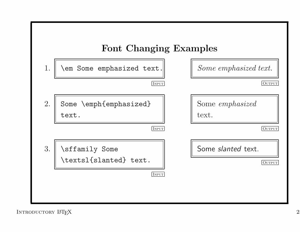
Font Changing Examples
1. \em Some emphasized text.
Input
Some emphasized text.
Output
2. Some \emph{emphasized}
text.
Input
Some emphasizedtext.
Output
3. \sffamily Some
\textsl{slanted} text.
Input
Some slanted text.
Output
Introductory LATEX 23

Font Changing Examples
4. \scshape Some more
\upshape text.
Input
Some more text.
Output
5. \itshape Some
\emph{emphasized} text.
Input
Some emphasized text.
Output
6. {\bfseries Some
bold} text.
Input
Some bold text.
Output
Introductory LATEX 24

Font Changing Environments
• Environments can also be used to change font locally.
• The name of the environment is the same as the declaration,without the preceding \.
• Example:
Some normal text.
\begin{bfseries}
Some bold text.
\end{bfseries}
Back to normal text.
Input
Some normal text. Somebold text. Back tonormal text.
Output
Introductory LATEX 25

Font Size Changing Declarations
\tiny tiny text
\scriptsize script sized text
\footnotesize footnote sized text
\small small text
\normalsize normal sized text
\large large text
\Large even larger
\LARGE larger still\huge huge\Huge really huge
Introductory LATEX 26

Font Size Changing Examples
1. Some normal sized text.
{\small Some small
text.}
Input
Some normal sizedtext. Some small text.
Output
2. Some \textbf{\large
large bold} text.
Input
Some large boldtext.
Output
Introductory LATEX 27
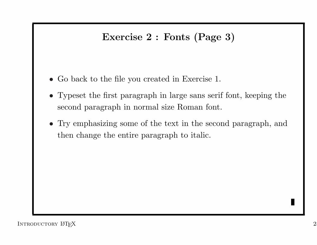
Exercise 2 : Fonts (Page 3)
• Go back to the file you created in Exercise 1.
• Typeset the first paragraph in large sans serif font, keeping thesecond paragraph in normal size Roman font.
• Try emphasizing some of the text in the second paragraph, andthen change the entire paragraph to italic.
Introductory LATEX 28

Symbols
\& & \_ \P ¶ - -
\# # \$ $ \dag † -- –
\{ { \pounds £ \ddag ‡ --- —
\} } \copyright c© \i ı ?‘ ¿
\% % \S § \j !‘ ¡
‘ ‘ ‘‘ “ ’ ’ ’’ ”
\ldots . . . \yen U
Introductory LATEX 29

Examples
1. \pounds 43.50
Input
£43.50
Output
2. See pages 23--30
Input
See pages 23–30
Output
3. A, B \& C
Input
A, B & C
Output
4. ‘‘She said to me:
‘is that it?’\,’’
Input
“She said to me: ‘isthat it?’ ”
Output
Introductory LATEX 30
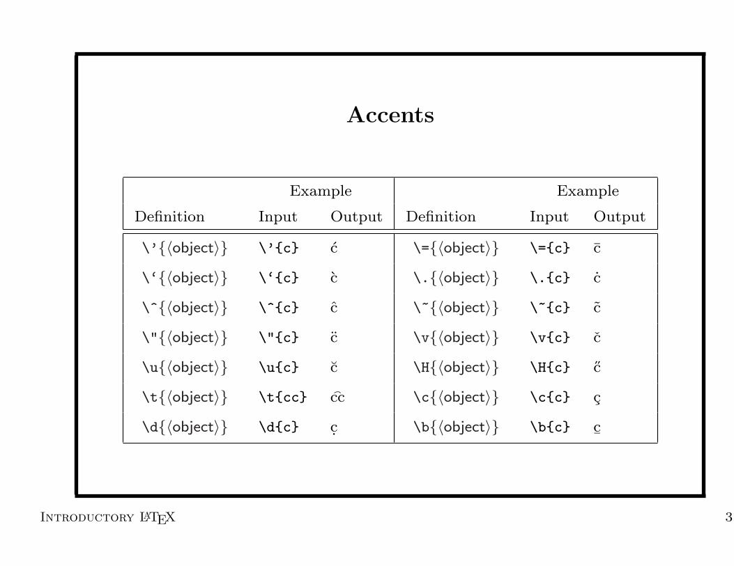
Accents
Example Example
Definition Input Output Definition Input Output
\’{〈object〉} \’{c} c \={〈object〉} \={c} c
\‘{〈object〉} \‘{c} c \.{〈object〉} \.{c} c
\^{〈object〉} \^{c} c \~{〈object〉} \~{c} c
\"{〈object〉} \"{c} c \v{〈object〉} \v{c} c
\u{〈object〉} \u{c} c \H{〈object〉} \H{c} c
\t{〈object〉} \t{cc} Äcc \c{〈object〉} \c{c} c
\d{〈object〉} \d{c} c. \b{〈object〉} \b{c} c¯
Introductory LATEX 31

Example of Words with Accents
1. Caf\’e
Input
Cafe
Output
2. R\^ole
Input
Role
Output
3. P\^at\’e
Input
Pate
Output
4. Na\"{\i}ve
Input
Naıve
Output
Introductory LATEX 32

Ligatures
\AE Æ \ae æ \OE Œ \oe œ
fi fi ffi ffi fl fl ffl ffl
Foreign Symbols
\AA A \aa a \L ÃL \l Ãl
\O Ø \o ø \ss ß
Introductory LATEX 33

Examples of Words Containing Ligatures
1. Man{\oe}uvre
Input
Manœuvre
Output
2. {\AE}olian
Input
Æolian
Output
3. {\OE}sophagus
Input
Œsophagus
Output
4. fluffier
Input
fluffier
Output
Introductory LATEX 34

Exercise 3 : Punctuation, Accents and Symbols
(Page 5)
Create a LATEX document that will produce the output shown inFigure 2 on page 5 of the handouts.
Make note of the following:
• Accent commands take one argument which must be thecharacter you want the accent over.
• If you want an accent over an i use a dotless i (ı).
• Remember to either group a command that produces a ligature,or place a space after it.
Introductory LATEX 35

Document Classes and Sectioning Commands
Standard Class Files
article report book slides letter
Standard Sectioning Commands
\part \subsubsection[〈short title〉]{〈Title〉}\chapter[〈short title〉]{〈Title〉} \paragraph{〈Title〉}\section[〈short title〉]{〈Title〉} \subparagraph{〈Title〉}\subsection[〈short title〉]{〈Title〉}
Introductory LATEX 36

Examples of Sectioning Commands
1. \section{Introduction}
\LaTeX\ documents
are\ldots
Input
1 Introduction
LATEX documents are. . .
Output
2. \subsection{Macros}
Macros\ldots
Input
1.1 Macros
Macros. . .
Output
3. \section*{Unnumbered
Sections}
Input
Unnumbered
SectionsOutput
Introductory LATEX 37

Abstract
• Some class files such as article and report define an abstract
environment.
• Example:
\begin{abstract}
This is the body of
the abstract.
The format depends
on the class
file you use.
\end{abstract}
Input
Abstract
This is the body
of the abstract. The
format depends on
the class file you use.
Output
Introductory LATEX 38

Title Pages and Table of Contents
• To create a title page, you first need to store information usingthe commands:
\author{〈Author Names〉}\title{〈Document Title〉}\date{〈Date〉}
• The information is then displayed using the command:
\maketitle
• The table of contents can be produced by using the command:
\tableofcontents
Introductory LATEX 39

Example Title Page
\author{N.L.C. Talbot}
\title{Introductory
\LaTeX}
\date{October 2002}
\maketitle
Input
Introductory
LATEX
N.L.C. Talbot
October 2002Output
Introductory LATEX 40

Appendices
• To switch to appendices, use the command:
\appendix
at the start of the appendices.
• Continue to use \chapter or \section commands, depending onthe class file.
Introductory LATEX 41

Example
% This is the 4th section
\section{Conclusions}
Here are the conclusions.
\appendix
\section{Tables}
This is the first appendix.
\section{Proofs}
This is the second
appendix.
Input
4 Conclusions
Here are the conclusions.
A Tables
This is the first appendix.
B Proofs
This is the second appendix.
Output
Introductory LATEX 42

Standard Class File Options
Some of the more common options:onecolumn Format document in one column format
twocolumn Format document in two column format
titlepage Make the title page appear on a separate page
notitlepage Make the title appear at the top of the first page of the
document
oneside Format the document for one-sided printing
twoside Format the document for two-sided printing
portrait Format the document in portrait orientation
landscape Format the document in landscape orientation
10pt Make the normal font be 10pt
11pt Make the normal font be 11pt
12pt Make the normal font be 12pt
Introductory LATEX 43

Page Styles
• Page numbers appear automatically
• By default, in the article class file the page numbers appearcentred in the footer.
• The page style (how headers and footers appear) can be changedusing the command:
\pagestyle{〈style〉}
• The most common styles are: plain, empty and headings.
Introductory LATEX 44

Exercise 4 : Sectioning Commands etc (Page 7)
• Copy over the file sectioning.tex following the instructions inthe handout. Load the file sectioning.tex into a text editor,and find the line that says:
% SECTION : Introduction
On the following line, insert the line
\section{Introduction}
• Go through the rest of the file, and insert the appropriatesectioning commands
• Make the table of contents appear, by placing the command\tableofcontents at the place where you want it to appear.
• Use \maketitle to make the title information appear.
Introductory LATEX 45

Paragraph Formatting
By default, paragraphs are fully justified, however the justificationcan be changed, either by a declaration, or an environment.
Declaration \flushleft \flushright \centering
Environment flushleft flushright centering
Introductory LATEX 46

Examples
• Only whole paragraphs can be justified.
{\flushright Some right
justified text.\par}
Input
Some right justifiedtext.
Output
• Alternatively:
\begin{flushright}
Some right
justified text.\par
\end{flushright}
Input
Some right justifiedtext.
Output
Introductory LATEX 47

Centering a Single Line of Text
There is also a command to centre a single line of text:
\centerline{〈text〉}
Example:
\centerline{Some centred text}
Input
Some centred text
Input
Introductory LATEX 48

New Lines
• To force a new line: \\[〈length〉] or \newline
• Line one\\
Line two\\[20pt]
Line three
Input
Line oneLine two
Line three
Output
• \flushright
Line one\\
Line two\\[20pt]
Line three\par
Input
Line oneLine two
Line three
Output
Introductory LATEX 49

Line breaks
• To break a line but keeping the text fully justified use:\linebreak[〈n〉]
• A short fully
justified paragraph.
Input
A short fully justifiedparagraph.
Output
• A short \linebreak fully
justified paragraph.
Input
A shortfully justified para-graph.
Output
Introductory LATEX 50

Preventing Line breaks
• To prevent a line break use: \nolinebreak[〈n〉]
• A short fully
justified paragraph.
Input
A short fully justifiedparagraph.
Output
• A short fully
justified\nolinebreak\
paragraph.
Input
A short fully justi-fied paragraph.
Output
Introductory LATEX 51

Unbreakable Spaces
Alternatively, use a tilde ~ to produce a space that can not bebroken by a new line. For example:
Numbers such as the 3
in Example 3, should
never occur at the
start of a new line.
Input
Numbers such as the 3 in Example3, should never occur at the startof a new line.
Output
Numbers such as the 3
in Example~3, should
never occur at the
start of a new line.
Input
Numbers such as the 3 in Exam-ple 3, should never occur at thestart of a new line.
Output
Introductory LATEX 52

Page Breaks
• To force a ragged page break, use:
\newpage
• To force a vertically justified page break, use:
\pagebreak[〈n〉]• To prevent a page break, use:
\nopagebreak[〈n〉]• To force a page break, and process all unprocessed floats, use:
\clearpage
Introductory LATEX 53

Exercise 5 : Paragraph Formatting (Page 9)
• Reproduce the output shown in Figure 3 on page 9 of thehandouts.
• First use declarations, then try using environments.
Introductory LATEX 54

Defining New Commands
• To define a new command use:
\newcommand{〈cmd-name〉}[〈nargs〉][〈default〉]{〈text〉}• 〈cmd-name〉 is the name of the new command (remember the
backslash)
• 〈nargs〉 is the numbers of arguments the new command takes(default 0)
• 〈default〉 is the default value for the first argument should anoptional argument be required
• 〈text〉 is what LATEX should do every time it encounters thiscommand.
• Never redefine a command whose existing meaning is unknownto you.
Introductory LATEX 55

Why Define New Commands?
• To reduce lengthy typing:
\newcommand{\introLaTeX}{%
\emph{Introductory \LaTeX}}
The \introLaTeX\ course
is run by CSED\ldots
Input
The Introductory LATEXcourse is run by CSED. . .
Output
Introductory LATEX 56

Why Define New Commands?
• To ensure consistency:
\newcommand{\envname}[1]{%
\textsf{#1}}
The \envname{abstract}
environment\ldots
Input
The abstract environ-ment. . .
Output
Introductory LATEX 57

Examples
% First define the new command
\newcommand{\price}[2]{\pounds #1.#2}
%
The price is \price{2}{50}.
Input
The price is £2.50.
Output
\newcommand{\cost}[2][17.5]{%
The cost is \pounds #2 excl.\ VAT
@ #1\%}
%
\cost{100}.\\
\cost[0.0]{50}
Input
The cost is £100 excl.
VAT @ 17.5%.
The cost is £50 excl.
VAT @ 0.0%
Output
Introductory LATEX 58

Exercise 6 : Defining New Commands (Page 11)
• Create a new document called exercise6.tex.
• Define the command \timeofday. This command should taketwo parameters, the first is the hour and the second is thenumber of minutes passed the hour. For example, the command\timeofday{10}{25} should produce the output: 10:25.
• Create the output shown in Figure 4 on page 11 where the timeis produced using the \timeofday command.
• Once you have done this, change the definition of the commandso that the time is displayed in bold.
Introductory LATEX 59
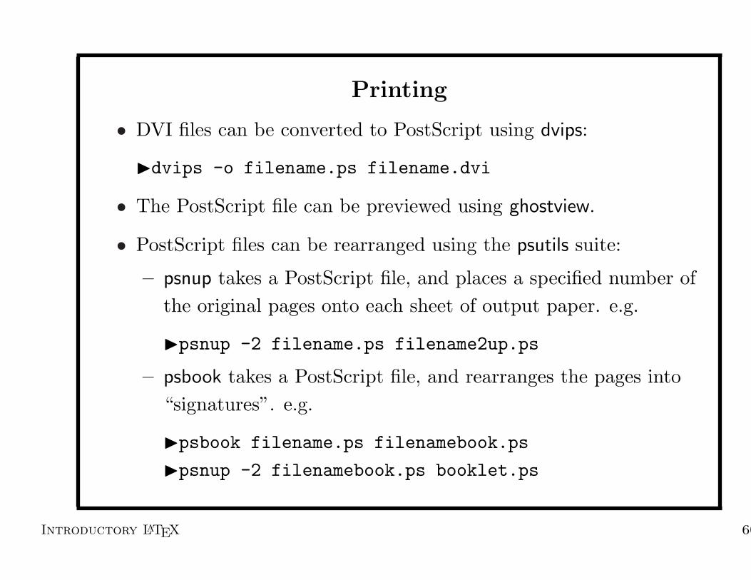
Printing
• DVI files can be converted to PostScript using dvips:
Idvips -o filename.ps filename.dvi
• The PostScript file can be previewed using ghostview.
• PostScript files can be rearranged using the psutils suite:
– psnup takes a PostScript file, and places a specified number ofthe original pages onto each sheet of output paper. e.g.
Ipsnup -2 filename.ps filename2up.ps
– psbook takes a PostScript file, and rearranges the pages into“signatures”. e.g.
Ipsbook filename.ps filenamebook.ps
Ipsnup -2 filenamebook.ps booklet.ps
Introductory LATEX 60

Exercise 7 (Page 12)
• Try converting the document (sectioning.tex) that youmodified in Exercise 4 into a PostScript file:
Idvips -o sectioning.ps sectioning
• Now view it using ghostview:
Ighostview sectioning.ps
Introductory LATEX 61

List Making Environments
The itemize environment produces an unordered list.
\begin{itemize}
\item The first item
\item The second item
\item The third item
\end{itemize}
Input
• The first item
• The second item
• The third item
Output
Introductory LATEX 62

Nested itemize environments
Up to four itemize environments may be nested:
\begin{itemize}
\item The first item
\begin{itemize}
\item First item
of nested list
\item Second item
of nested list
\end{itemize}
\item The second item
\end{itemize}
Input
• The first item
– First item of nested list
– Second item of nestedlist
• The second item
Output
Introductory LATEX 63

Numbered Lists
The enumerate environment produces an ordered list.
\begin{enumerate}
\item The first item
\item The second item
\item The third item
\end{enumerate}
Input
1. The first item
2. The second item
3. The third item
Output
Introductory LATEX 64

Nested enumerate environments
Up to four enumerate environments may be nested:
\begin{enumerate}
\item The first item
\begin{enumerate}
\item First item
of nested list
\item Second item
of nested list
\end{enumerate}
\item The second item
\end{enumerate}
Input
1. The first item
(a) First item of nested list
(b) Second item of nestedlist
2. The second item
Output
Introductory LATEX 65

Nested itemize and enumerate environments
itemize and enumerate environments may be nested:
\begin{enumerate}
\item The first item
\begin{itemize}
\item First item
of nested list
\item Second item
of nested list
\end{itemize}
\item The second item
\end{enumerate}
Input
1. The first item
• First item of nested list
• Second item of nestedlist
2. The second item
Output
Introductory LATEX 66

Description
\begin{description}
\item[Cabbage] A large
round green vegetable
\item[Brussel sprout] A
small round
green vegetable
\end{description}
Input
Cabbage A large roundgreen vegetable
Brussel sprout Asmall round greenvegetable
Output
Introductory LATEX 67

Exercise 8 : Lists (Page 12)
• Create a document that produces the output shown in Figure 5on page 13 of the handouts.
• You will need to use an enumerate environment and nesteditemize environments.
• The default labels for each level of nested itemize environmentsare: • – ∗ and ·. The corresponding commands used to produceeach label are: \labelitemi \labelitemii \labelitemiii and\labelitemiv. These can be redefined, e.g.
\renewcommand{\labelitemi}{\S}
but they must be redefined prior to use.
Introductory LATEX 68

Tabulated Material
Material can be aligned in rows and columns using the tabular
environment.
\begin{tabular}{lc}
Item & Cost\\
CD & \pounds 11.75\\
Video & \pounds 14.10\\
Total & \pounds 25.85
\end{tabular}
Input
Item Cost
CD £11.75
Video £14.10
Total £25.85
Output
Introductory LATEX 69

Adding Horizontal and Vertical Lines
\begin{tabular}{|l|c|}
\hline
Item & Cost\\\hline\hline
CD & \pounds 11.75\\
Video & \pounds 14.10\\\hline
Total & \pounds 25.85\\\hline
\end{tabular}
Input
Item Cost
CD £11.75
Video £14.10
Total £25.85
Output
Introductory LATEX 70

\begin{tabular}{|l|cc|}\hline
& \multicolumn{2}{c|}{Cost}\\
Item & ex VAT & inc VAT (@17.5\%)\\\hline\hline
CD & \pounds 10.00 & \pounds 11.75\\
Video & \pounds 12.00 & \pounds 14.10\\\hline
\multicolumn{1}{l|}{Total} & \pounds 22.00 &
\pounds 25.85\\\cline{2-3}
\end{tabular}
Input
Cost
Item ex VAT inc VAT (@17.5%)
CD £10.00 £11.75
Video £12.00 £14.10
Total £22.00 £25.85
Output
Introductory LATEX 71

Exercise 9 : Tabulated Material (Page 14)
• Create the table shown in Figure 6 on page 15 of the handouts.
• The table is created using just one tabular environment. Thelines Equipment Expenditure and Travel Expenditure spanall 5 columns.
• It’s best to start with a simple table, and then gradually add themore complicated bits.
• Once you’ve finished it, centre the table, using the \centerline
command.
Introductory LATEX 72

Basic Mathematics
• In-line maths:\begin{math} . . . \end{math}
\( . . . \)
$ . . . $
• One line of displayed maths:
\begin{equation} . . . \end{equation}
\begin{displaymath} . . . \end{displaymath}
\[ . . . \]
Introductory LATEX 73

Examples
I can refer to the
variable $x$, or the
formula \(y = mx+c\).
Input
I can refer to the variable x,or the formula y = mx + c.
Output
The function is:
\[f(x) = 4x + 1\]
Input
The function is:
f(x) = 4x + 1
Output
\begin{equation}
f(x) = 4x + 1
\end{equation}
Input
f(x) = 4x + 1 (1)
Output
Introductory LATEX 74

Subscripts and Superscripts
• Subscripts are created using the command _{〈subscript〉}
• Superscripts are created using the command ^{〈superscript〉}• Example:
\begin{displaymath}
y = a_0 + a_1 x + a_2 x^2
\end{displaymath}
Input
y = a0 + a1x + a2x2
Output
• Nested superscripts or subscripts should be grouped to avoid
confusion:
Compare $a_b^c$ with $a_{b^c}$.
Input
Compare acb with abc .
Output
Introductory LATEX 75

Fractions and Square Roots
• Fractions are produced using:\frac{〈numerator〉}{〈denominator〉}
• Roots are produced using:\sqrt[〈n〉]{〈maths〉}
• Example:
\begin{displaymath}
f(x_1, x_2) = x_1^2
+ e^{x_2} +
\frac{\sqrt[3]{a}}%
{1+\sqrt{x_2}}
\end{displaymath}
Input
f(x1, x2) = x21+ex2+
3√
a
1 +√
x2
Output
Introductory LATEX 76

Greek Letters and Log-like Symbols
• Greek letters can be produced by typing a backslash followed bythe Greek name, e.g. \alpha produces α.
• Capitalizing the first letter will produce the upper case character.e.g. \Gamma produces Γ.
• Log-like symbols such as log and sin, can simply be producedusing the commands \log, \sin, etc.
\begin{displaymath}
e^{i\theta} = \cos\theta
+ i\sin\theta
\end{displaymath}
Input
eiθ = cos θ + i sin θ
Output
Introductory LATEX 77

Summations, Products and Limits
• Summations and products can be produced using the commands:\sum_{〈start〉}^{〈end〉}\prod_{〈start〉}^{〈end〉}
• Limits are produced using the command:\lim_{〈limit〉}
\begin{displaymath}
\lim_{\theta\rightarrow\pi}
\sum_{i=1}^{n}
\theta^i\sin\theta
\end{displaymath}
Input
limθ→π
n∑
i=1
θi sin θ
Output
Introductory LATEX 78

Examples
\begin{displaymath}
f(x) = \sum_{i=0}^{n}
\alpha_i \xi^i
\end{displaymath}
Input
f(x) =n∑
i=0
αiξi
Output
In text :
\begin{math}
f(x) = \sum_{i=0}^n
\alpha_i \xi^i
\end{math}
Input
In text : f(x) =∑n
i=0 αiξi
Output
Introductory LATEX 79

Exercise 10 : Basic Mathematics (Page 16)
• Produce the output shown in Figure 7 on page 16 of thehandouts.
• Remember to typeset the f(x), f and x in the text in mathsmode.
• Try making the equation a numbered equation.
Introductory LATEX 80

Delimiters
• Placing brackets around a tall object in maths mode, such asfractions, does not look right if you use normal sized brackets.For example:
\begin{displaymath}
(\frac{1}{1+x})
\end{displaymath}
Input
(1
1 + x)
Output
• Under such circumstances, it is better to use the commands:\left〈delimiter〉 and \right〈delimiter〉
• Note that you must always have matching \left and \right
commands, although the delimiters used may be different.
Introductory LATEX 81

Delimiters
( ( ) ) [ [ ] ]
\{ { \} } | | \| ‖/ / \backslash \ \langle 〈 \rangle 〉\lfloor b \rfloor c \lceil d \rceil e\uparrow ↑ \downarrow ↓ \Uparrow ⇑ \Downarrow ⇓\updownarrow l \Updownarrow m
If you want one of the delimiters to be invisible, use a . (full stop) asthe delimiter.
Introductory LATEX 82

Examples
\begin{displaymath}
\left(
\frac{1}{1+x}
\right)
\end{displaymath}
Input
(1
1 + x
)
Output
\begin{displaymath}
\left|
\frac{1}{1+x}
\right|
\end{displaymath}
Input
∣∣∣∣1
1 + x
∣∣∣∣
Output
Introductory LATEX 83

Arrays
• Arrays can be created using the array environment.
• Similar to the tabular environment, but must be in maths mode.
• Elements are arranged in rows and columns to formmathematical structures such as vectors and matrices.
Introductory LATEX 84

\begin{displaymath}
\begin{array}{cc}
0 & 1 \\
2 & 3
\end{array}
\end{displaymath}
Input
0 1
2 3
Output
\begin{displaymath}
\left (
\begin{array}{cc}
0 & 1 \\
2 & 3
\end{array}
\right )
\end{displaymath}
Input
0@ 0 1
2 3
1AOutput
Introductory LATEX 85

\begin{displaymath}
\left[
\begin{array}{cc}
0 & 1 \\
2 & 3
\end{array}
\right\}
\end{displaymath}
Input
0 1
2 3
Output
Introductory LATEX 86

\begin{displaymath}
f(x) =
\left \{
\begin{array}{cl}
0 & x \leq 0 \\
1 & x > 0
\end{array}
\right .
\end{displaymath}
Input
f(x) =
0 x ≤ 0
1 x > 0
Output
Introductory LATEX 87

Exercise 11 : Arrays (Page 18)
• Create the output shown in Figure 8 on page 18 of the handouts.
• You will need the following commands:
\cdots · · ·\vdots
...
\ddots. . .
\neq 6=
Introductory LATEX 88

Multiline Formulæ
• The displaymath and equation environments only allow one line ofmathematics.
• The eqnarray environment allows multiple equations to bealigned.
• The eqnarray environment has three columns: the first is rightaligned, the second is centrally aligned and the third is leftaligned.
• Each line is numbered in the eqnarray environment.
• The eqnarray* environment is unnumbered.
• To suppress line numbering in the eqnarray, use the command\nonumber on the appropriate line.
Introductory LATEX 89

\begin{eqnarray}
\ln(f(x)) & = & x^2 + \frac{1}{x+3}\\
f(x) & = & \exp \left ( x^2
+ \frac{1}{x+3} \right )
\end{eqnarray}
Input
ln(f(x)) = x2 +1
x + 3(2)
f(x) = exp(
x2 +1
x + 3
)(3)
Output
Introductory LATEX 90

\begin{eqnarray}
\ln(f(x)) & = & x^2 + \frac{1}{x+3} \nonumber\\
f(x) & = & \exp \left ( x^2
+ \frac{1}{x+3} \right )
\end{eqnarray}
Input
ln(f(x)) = x2 +1
x + 3
f(x) = exp(
x2 +1
x + 3
)(4)
Output
Introductory LATEX 91

Exercise 12 : Multiline Formulæ (Page 19)
• Produce the output shown in Figure 9 on page 19 of thehandouts.
• You will need the following commands:
\approx ≈ \pm ±\partial ∂ \leq ≤\varepsilon ε
Introductory LATEX 92

Cross-Referencing
• Assign a textual label using \label{〈string〉}Example:
\section{Introduction}
\label{sec:intro}
Example:
\begin{equation}
E = mc^2
\label{eqn:einstein}
\end{equation}
• Refer to the object using \ref{〈string〉} .
• Refer to the page that the object is on using\pageref{〈string〉} .
Introductory LATEX 93

Examples
\section{Introduction}
\label{sec:intro}
\ldots
See Section~\ref{sec:intro}
for a brief introduction.
Input
1 Introduction. . . See Section 1 for abrief introduction.
Output
\subsection{Examples}
\label{sec:ex}
\ldots
See subsection~\ref{sec:ex}
for examples.
Input
2.3 Examples. . . See subsection 2.3for examples.
Output
Introductory LATEX 94

Examples
See Appendix~\ref{apd:tables}
for tables\ldots
\appendix
\section{Tables}\label{apd:tables}
Input
See Appendix A for ta-
bles. . .
A Tables
Output
\begin{equation}
\label{eqn:Emc}
E = mc^2
\end{equation}
\ldots
See Equation~\ref{eqn:Emc}
on page~\pageref{eqn:Emc}.
Input
E = mc2 (5)
. . . See Equation 5 on
page 95.
Output
Introductory LATEX 95

Exercise 13 (Page 20)
• Reproduce the document shown in Figure 10 on page 21 of thehandouts using \label and \ref. You will need to rememberhow to:
– create sections
– emphasize text
– create numbered equations
– have in-line mathematics
• Try adding a title and table of contents
• Try inserting an extra section between the introductory sectionand the section on Bayes’ Theorem, and try inserting anotherequation, to see how LATEX automatically updates thecross-references.
Introductory LATEX 96

Packages
• Packages are files with the extension .sty
• Packages can redefine existing commands, or provide newcommands.
• Any package you may wish to use with your document must bespecified with the command
\usepackage[〈options〉]{〈package-name〉}
This command can only be used in the preamble.
Introductory LATEX 97
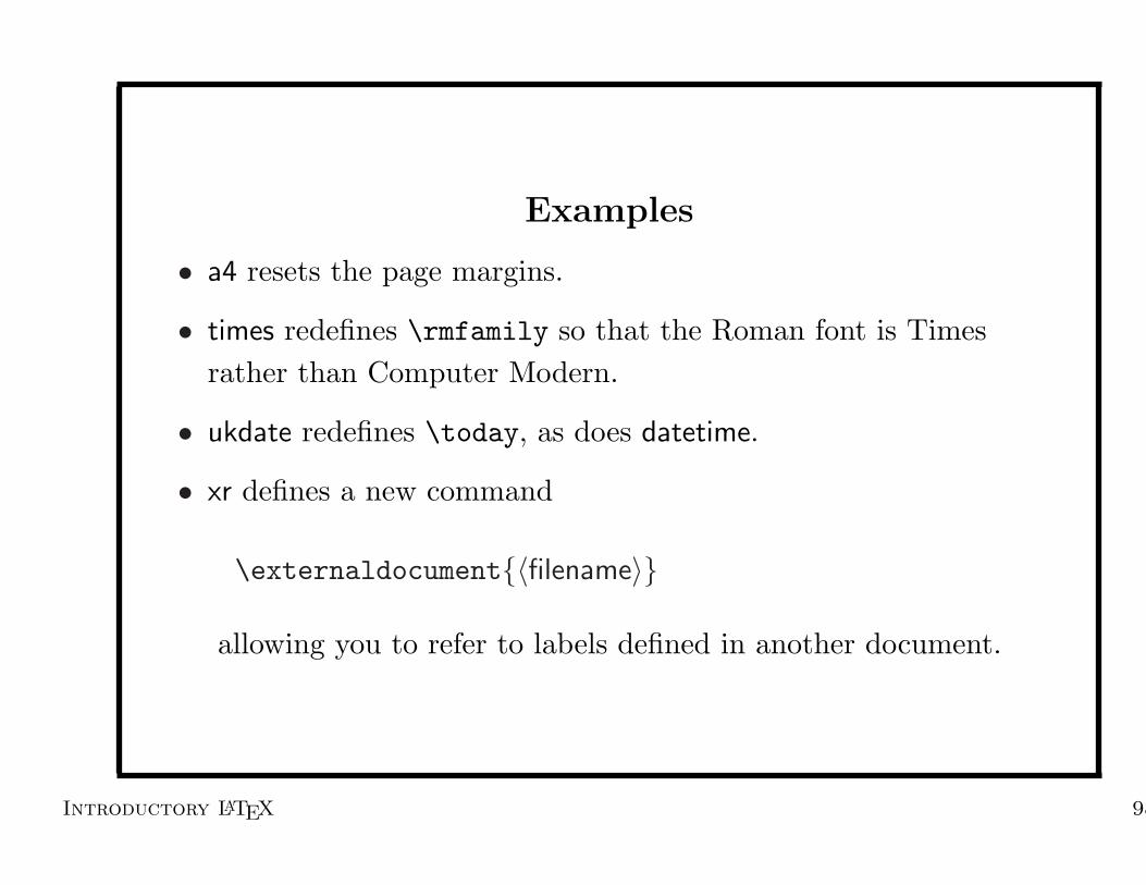
Examples
• a4 resets the page margins.
• times redefines \rmfamily so that the Roman font is Timesrather than Computer Modern.
• ukdate redefines \today, as does datetime.
• xr defines a new command
\externaldocument{〈filename〉}
allowing you to refer to labels defined in another document.
Introductory LATEX 98

Example
\documentclass[a4paper]{article}
\begin{document}
\today
\end{document}
Input
April 29, 2003
Output
\documentclass[a4paper]{article}
\usepackage[short]{datetime}
\begin{document}
\today
\end{document}
Input
Tue 29th Apr, 2003
Output
Introductory LATEX 99

Self-Extracting Documentation
• Packages not currently on your TEX installation can bedownloaded from the TEX archive.
• Increasingly packages are bundled up with their documentationin a file with the extension .dtx
• The package should also come with a driver or installation script(.ins)
• The documentation can usually be obtained by LATEXing the.dtx file. For example:Ilatex datetime.dtx
• The package can be extracted by LATEXing the installation script.For example:Ilatex datetime.ins
Introductory LATEX 100

Exercise 14 (Page 22)
• Go back to the document from the previous exercise.
• Typeset the first paragraph in Times Roman instead of thedefault Computer Modern Roman.
• Typeset the second paragraph in Avant Garde — defined in thefile avant.sty. (Hint : Avant Garde is a sans serif font.)
• Change the way today’s date is formatted using ukdate package.
• If you want to try extracting documentation and code from a.dtx file, you can copy the datetime package over:
Icp /home/sys/gcc/insecure/datetime.* .
Introductory LATEX 101

Citations
• thebibliography environment
\begin{thebibliography}{2}
\bibitem{clarke83} G. M. Clarke and D. Cooke.
\emph{A basic course in statistics}.
Chapman and Hall, 2nd edition, 1983.
\bibitem{goossens93} M. Goossens and F. Mittelbach.
\emph{The \LaTeX\ companion}.
Addison-Wesley, 1993.
\end{thebibliography}
• Use \cite[〈text〉]{〈key〉} to cite a reference in the bibliography
Introductory LATEX 102

Example
See Goossens \emph{et
al.}~\cite{goossens93}
\ldots
\begin{thebibliography}{2}
\bibitem{goossens93}
M. Goossens and
F. Mittelbach.
\emph{The \LaTeX\
companion}.
Addison-Wesley, 1993.
\end{thebibliography}
Input
See Goossens et al. [1]. . .
References
[1] M. Goossens andF. Mittelbach. TheLATEX companion.Addison-Wesley,1993.
Output
Introductory LATEX 103

BiBTEX
Use BiBTEX to automatically generate thebibliography environment.
• Large database containing many references.
• BiBTEX will only include those that are cited in the document.
• Entries sorted.
• Entries consistently formatted.
Introductory LATEX 104

Bibliography Database (.bib)
@entry type{keyword,
field = "text",...
field = "text"
}@book{kreyszig88,
author = "Kreyszig, Erwin",
title = "Advanced Engineering Mathematics",
publisher = "Wiley",
edition = "6th",
year = 1988
}
Introductory LATEX 105

Author Format
Authors should be entered in one of the following formats:
• 〈forenames〉 〈von〉 〈surname〉• 〈von〉 〈surname〉, 〈forenames〉• 〈von〉 〈surname〉, 〈jr〉, 〈forenames〉
Examples:
Entry Output (“abbrev” style)
"Alex Thomas von Neumann" A.T. von Neumann
"John Chris {Smith Jones}" J.C. Smith Jones
"van de Klee, Mary-Jane" M.-J. van de Klee
"Smith, Jr, Fred John" F.J. Smith, Jr
"Maria {\uppercase{d}e La} Cruz" M. De La Cruz
Compare last example with:
"Maria De La Cruz" M. D. L. Cruz (Incorrect!)
Introductory LATEX 106

Multiple Authors
Multiple authors should be separated by the keyword and
@book{goossens97,
author = "Goossens, Michel and Rahtz, Sebastian and
Mittelbach, Frank",
title = "The \LaTeX\ graphics companion: illustrating
documents with \TeX\ and {PostScript}",
publisher = "Addison Wesley Longman, Inc",
year = 1997
}
Introductory LATEX 107

Month Entries
• Bibliography styles always have three-letter abbreviations formonths: jan, feb, mar, . . .
• Always use these abbreviations for consistency.
@inproceedings{talbot97,
author = "Talbot, Nicola and Cawley, Gavin",
title = "A fast index assignment algorithm for
robust vector quantisation of image data",
booktitle = "Proceedings of the I.E.E.E. International
Conference on Image Processing",
address = "Santa Barbara, California, USA",
month = oct,
year = 1997
}
Introductory LATEX 108

Example (incollection)
@incollection{wainwright,
author = "Wainwright, Robert B.",
title = "Hazards from {Northern} Native Foods",
booktitle = "\emph{Clostridium botulinum}: Ecology and
Control in Foods",
chapter = 12,
pages = "305--322",
editor = "Hauschild, Andreas H. W. and Dodds,
Karen L.",
publisher = "Marcel Dekker, Inc",
year = 1993
}
Introductory LATEX 109

Declaring Databases and Bibliography Style
In your LATEX source code (.tex):
• Declare the bibliography style:\bibliographystyle{〈style-name〉}
Common Styles:plain Entries sorted alphabetically with numeric labels.
unsrt Entries printed in order of citation with numeric labels.
alpha Entries sorted alphabetically with labels formed fromauthor’s name and year of publication.
abbrev Entries sorted alphabetically with first name, month andjournal names abbreviated.
• Declare the bibliography database:\bibliography{〈name〉}
Introductory LATEX 110

Example
In filename.tex (where database.bib contains the bibliographydatabase):
This is the document \ldots
\bibliographystyle{plain}
\bibliography{database}
Input
At the command prompt:Ilatex filename
Ibibtex filename
Ilatex filename
Ilatex filename
Introductory LATEX 111

LATEX/BiBTEX Process
-
?
?
LATEX
BiBTEX
LATEX
.tex .aux .bib
.bbl
Introductory LATEX 112

Exercise 15 (Page 24)
• Produce a BiBTEX database that contains the references shownin Figure 11 on page 25, and create the document shown in thatfigure.
• Try changing the bibliography style so that the entries areprinted in order of citation. (You need the unsrt style for this).Try other styles, such as alpha, abbrv and acm, to see thedifferences between styles.
• If you have a number of citations, such as [3,2,4], you mightprefer to have it printed as a range, such as [2–4], instead. Thereis a package called citesort that redefines the \cite commandthat will do this. Try using this package with the unsrt
bibliography style.
Introductory LATEX 113

Lengths
• LATEX has commands that represent lengths, such as \textwidth.
• There are two types of lengths: rigid and rubber.
• A rigid length is a fixed length, such as 4in,
• a rubber length is a length with a certain amount of elasticity,for example 2in plus 0.1in minus 0.1in. A rubber length is away of telling LATEX your preferred length, and the amount ofdeviation from that length which you are prepared to put upwith. Most LATEX lengths are rigid lengths.
Introductory LATEX 114

Units
pt Point ( 172.27 in)
bp Big point, or PostScript point ( 172 in)
mm Millimetre (2.845pt)
cm Centimetre (28.45pt)
in Inch (25.4mm)
ex Height of lowercase x in current font
em Width of capital M in current font
Introductory LATEX 115

Changing Lengths
• A length can be assigned a new value using the command:
\setlength{〈cmd〉}{〈length〉}
For example:
\setlength{\textwidth}{6in}
• A length can be incremented using the command:
\addtolength{〈cmd〉}{〈length〉}
so to make the text width 1in wider than it was previously, do:
\addtolength{\textwidth}{1in}
Introductory LATEX 116

Lengths
• There are three more commands that can change a length, andthey are:
\settowidth{〈cmd〉}{〈text〉}\settoheight{〈cmd〉}{〈text〉}\settodepth{〈cmd〉}{〈text〉}
These set the length 〈cmd〉 to the width, height or depth of the〈text〉. Note that the actual text itself is not typeset.
• To create a new length:
\newlength〈cmd〉• To display the value of a length:
\the〈cmd〉
Introductory LATEX 117

Example
% define new length
\newlength\mylen
% set it to the width of the text
\settowidth{\mylen}{Hello}
% Display the value
Width = \the\mylen.
Input
Width = 22.50005pt.
Output
Introductory LATEX 118

Layout Lengths
����������
��� ��
����������
��������� ����������
� ! "
��#
$
%
�'&! "
!"�(� &*)! "
!"�+
%
$� &�&
�,
$
%
%$��-
%$�.
%$
�/
021�3�465�3�78:9<;�8=1'>�>=?'4�@ AB1�3�4<5�3�78<9C;'D�1'>�>=?'4�@EF;�1'G�G=?H5GH4�I=J'K�L�5�3NMCO�E'PH@ QR;'@�1P�I=J�K�L�5�36MN0�S�PH@OF;�8�4�J�G�8�4=5L�8�@<MN0�A'PH@ TB;�8�4�J�G=?'4'P6M:A�O'PH@SF;'@H4�U�@�8�4=5L�8�@<MCO�V�W'PH@ WB;'@H4'U�@�X�5G�@�86MCE�Q�O'PH@VF;I=J�K�L�5�3�P�J�K�?'4'PNM60�0�PH@ 0�YB;I=J'K�L�5�3�P�J�K�X�5G�@�8NM:O�S'PH@0�02;'>�1�1'@=?Z�5�P<M:E�Y'PH@ ;I=J'K�L�5�3�P�J�K�P�[�?86MCO'PH@]\*3=1'@6?�8=1�X�3�^
;�8=1'>�>=?'4�@CM:Y'PH@ ;'D�1�>�>=?'4�@<M:Y'PH@;�P�J'P�4�K�X�5G�@'86MCO�V�S'PH@ ;�P�J�P�4�K�8�4=5L�8H@6M_W�QHO'PH@
1 one inch + \hoffset
2 one inch + \voffset
3 \oddsidemargin
4 \topmargin
5 \headheight
6 \headsep
7 \textheight
8 \textwidth
9 \marginparsep
10 \marginparwidth
11 \footskip
Introductory LATEX 119

Exercise 16 (Page 28)
• Go back to the document you created in Exercise 1
• Change the page layout dimensions so that the document is onA4 paper with 1in margins.
• Change the paragraph indentation (\parindent) to 0pt
• Change the gap between paragraphs (\parskip) to 3ex.
Introductory LATEX 120

Boxes and Minipages
• Boxes are treated as a single object.
• They can appear in the middle of a line.
• They can never be broken across a line.
• They can be vertically aligned:
– centrally :
– along the bottom :
– along the top :
Introductory LATEX 121

Basic Types of Boxes
• \mbox{〈contents〉}Simplest type of box.
– Prevents text inside it from being broken across a line
– Provides normal text inside a maths environment.
– Dimensions of the box automatically computed to fit thecontents of the box.
• \makebox[〈width〉][〈alignment〉]{〈contents〉}Like \mbox, but you can specify the width of the box, and howthe text is justified within it.
Introductory LATEX 122

Examples
\begin{displaymath}
y = x \mbox{ and }
z = x + y
\end{displaymath}
Input
y = x and z = x + y
Output
Box some in-line
$x = 1, \ldots, n$ maths.
Input
Box some in-line x =
1, . . . , n maths.
Output
Box some in-line
\mbox{$x = 1, \ldots, n$}
maths.
Input
Box some in-line
x = 1, . . . , n maths.
Output
Introductory LATEX 123

Examples
Here is \makebox[1in][r]{\em a 1in} box
Input
Here is a 1in box
Output
\makebox[0pt][l]{/////}Hello!
Input
/////Hello!
Input
Introductory LATEX 124

Boxes with Frames
\fbox and \framebox : These are the same as \mbox and \makebox,but they put a rectangular frame around the box.
Here is a \fbox{box}
Input
Here is a box
Output
Here is \framebox[1in][r]{\em a 1in} box
Input
Here is a 1in box
Output
Introductory LATEX 125

fancybox package
The fancybox package provides the following commands, that work inthe same way as \fbox, but produce different types of frames:
Input Output
\ovalbox{An oval frame}¤£
¡¢An oval frame
\Ovalbox{A thicker oval frame}¤£
¡¢A thicker oval frame
\doublebox{A double frame} A double frame
\shadowbox{A shadow frame}A shadow frame
Introductory LATEX 126

Examples
Here is a \ovalbox{box}
Input
Here is a¤£
¡¢box
Output
Here is \ovalbox{\makebox[1in][r]{\em a 1in}}
box
Input
Here is¤£
¡¢a 1in box
Output
Introductory LATEX 127

Examples
Here is a \Ovalbox{box}
Input
Here is a¤£
¡¢box
Output
Here is \Ovalbox{\makebox[1in][r]{\em a 1in}}
box
Input
Here is¤£
¡¢a 1in box
Output
Introductory LATEX 128

Examples
Here is a \doublebox{box}
Input
Here is a box
Output
Here is \doublebox{\makebox[1in][r]{\em a 1in}}
box
Input
Here is a 1in box
Output
Introductory LATEX 129
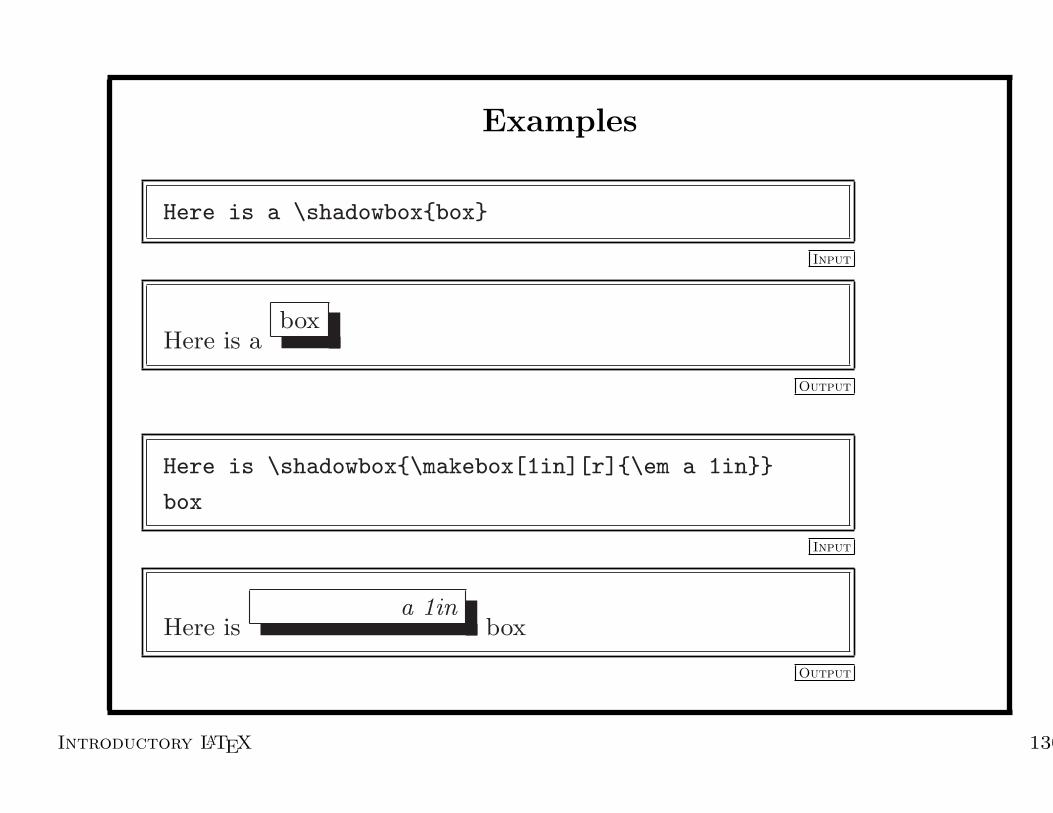
Examples
Here is a \shadowbox{box}
Input
Here is abox
Output
Here is \shadowbox{\makebox[1in][r]{\em a 1in}}
box
Input
Here isa 1in
box
Output
Introductory LATEX 130

Typesetting a Paragraph Inside a Box
\parbox[〈alignment〉][〈height〉]{〈width〉}{〈contents of box〉}
For example:
A paragraph within a box : \parbox{0.75in}{This box is
three quarters of an inch wide} so there!
Input
A paragraph within a box :
This box isthree quar-ters of aninch wide
so there!
Output
Introductory LATEX 131

The minipage Environment
\begin{minipage}[〈alignment〉][〈height〉]{〈width〉}
Some text. \begin{minipage}{0.4\textwidth} This width of this
minipage is 0.4 times the width of the text body\footnote{Note
we can also have a footnote}.
\end{minipage} Some more text.
Input
Some text.
This width of this minipage
is 0.4 times the width of the
text bodya.
aNote we can also have a
footnote
Some more text.
Output
Introductory LATEX 132

Raising and Lowering Boxes
• Boxes can be raised or lowered
• Syntax: \raisebox{〈lift〉}[〈depth〉][〈height〉]{〈contents〉}
some text \raisebox{2ex}{some raised}
\raisebox{-1ex}{some lowered}
Input
some textsome raised
some lowered
Output
Introductory LATEX 133

Rules
• A rule is a rectangular blob of ink
• Syntax: \rule[〈lift〉]{〈width〉}{〈height〉}
Some text
\rule{0.5in}{10pt}
\rule[-3pt]{0.5in}{10pt}
some text.
Input
Some text some text.
Output
Introductory LATEX 134

Example
\newlength\mylen
\settowidth{\mylen}{Some Text}%
\makebox[0pt][l]{\rule[0.5ex]{\mylen}{1pt}}%
Some Text
Input
Some Text
Output
Introductory LATEX 135

Example
\newlength\mylen
\newcommand{\strikethrough}[1]{%
\settowidth{\mylen}{#1}%
\makebox[0pt][l]{\rule[0.5ex]{\mylen}{1pt}}%
#1}
\strikethrough{Some More Text}
Input
Some More Text
Output
Introductory LATEX 136

Struts
A zero width rule is called a strut :
\fbox{text}
\fbox{\rule[-10pt]{0pt}{20pt}text}
text\rule{1in}{0pt}text
Input
text text text text
Output
Introductory LATEX 137

Saveboxes
• A savebox allows you to save some typeset text for later use.
• Define new savebox: \newsavebox{cmd}.
• To save text to a savebox:
– command:\sbox{〈cmd〉}{〈text〉}
– environment:\begin{lrbox}{〈cmd〉}〈text〉\end{lrbox}
• To display the contents of a savebox: \usebox{〈cmd〉}
Introductory LATEX 138

Example
\newsavebox{\mysbox}
\sbox{\mysbox}{Some interesting text}
\usebox{\mysbox}\\
\fbox{\usebox{\mysbox}}\\
\Ovalbox{\usebox{\mysbox}}
Input
Some interesting textSome interesting text¨
§¥¦Some interesting text
Output
Introductory LATEX 139

Example
\newsavebox{\mysbox}
\begin{lrbox}{\mysbox}
Some more interesting text.
\end{lrbox}
\usebox{\mysbox}\\
\fbox{\usebox{\mysbox}}
Input
Some more interesting text.Some more interesting text.
Output
Introductory LATEX 140

Macros verses Saveboxes
Using a macro (or command):
\newcommand{\sometext}{Some text}
\sometext.\\
\sffamily \sometext.\\
\ttfamily \sometext.
Input
Some text.Some text.
Some text.
Output
TEX has to work out how to typeset “Some text” three times.
Introductory LATEX 141

Macros verses Saveboxes
Using a savebox:
\newsavebox{\mysbox}
\sbox{\mysbox}{Some text}
\usebox{\mysbox}.\\
\sffamily \usebox{\mysbox}.\\
\ttfamily \usebox{\mysbox}.
Input
Some text.Some text.Some text.
Output
TEX only has to work out how to typeset “Some text” once.
Introductory LATEX 142

Exercise 17 (Page 30)
• Try reproducing the output shown in Figure 13 on Page 30 of thehandout.
• Try changing the vertical alignment of the minipage.
• Try experimenting with footnotes insides and outside of theminipage environment.
• Try using a \parbox instead of a minipage.
• Try experimenting with different frames around the minipage.
Introductory LATEX 143

Incorporating PostScript Pictures
• PostScript pictures are a convenient way of including graphicsinto a LATEX document.
• PostScript files can be created using a normal graphicsapplication, and printing to a file using a PostScript printerdriver. Some graphics applications have an option to save animage as a PostScript file.
• A PostScript file can be included into a LATEX document usingthe command
\includegraphics[〈options〉]{〈filename〉}
supplied by the package graphicx.
Introductory LATEX 144

Syntax
\includegraphics[〈options〉]{〈filename〉}Some of the more common options are:
angle=〈x〉 rotate the picture by 〈x〉◦width=〈len〉 scale the picture so that the width is 〈len〉.height=〈len〉 scale the picture so that the height is 〈len〉.scale=〈x〉 scale the picture.
bb=〈lx〉 〈by〉 〈rx〉 〈ty〉 set the bounding box so that the bottom leftco-ordinate is (〈lx〉, 〈by〉) and the top rightco-ordinate is (〈rx〉, 〈ty〉).
clip clip the picture.
draft don’t display the image, just draw the bound-ing box with the filename inside.
Introductory LATEX 145

An Example
\includegraphics[angle=90,width=1in]{shapes.ps}
Input
Output
Introductory LATEX 146

Exercise 18 (Page 32)
• Copy the file shapes.ps to your directory (following theinstructions in the handout), and include it in a document.
• Try to centre the image, using \centerline.
• Try putting a frame around it.
• Try scaling and rotating it.
• Try passing the option draft to the graphicx package and seewhat happens.
Introductory LATEX 147

Figures and Tables
• Figures and Tables are floats — they are floated to the nearestconvenient location according to certain typographical rules.
• A figure or table has a caption and an associated number.Captions are produced using the command:\caption[〈short caption〉]{〈caption text〉}
• LATEX handles numbering automatically. Floats can becross-referenced using \label and \ref.
• Figures are created using the figure environment.
• Tables are created using the table environment.
• figure and table environments can not have a page break in them.
Introductory LATEX 148

An Example Figure
\begin{figure}[tbh]
\centerline{\includegraphics[height=1.25cm]{shapes.ps}}
\caption{Some shapes}
\label{fig:shapes}
\end{figure}
Input
Figure 1: Some shapes
Output
Introductory LATEX 149

An Example Table
\begin{table}[tbh]
\caption{An example table}
\label{tab:example}
\vspace{10pt}
\centerline{
\begin{tabular}{l|ll}
& A & B\\\hline
I & 0.5 & 1.0\\
II & 12 & 14
\end{tabular}
}
\end{table}
Input
Table 1: An example table
A B
I 0.5 1.0
II 12 14
Output
Introductory LATEX 150

Adjacent Figures
Two figures can be placed side by side in one figure environment:
\begin{figure}[tbh]
\begin{minipage}{0.4\textwidth}
\centerline{\includegraphics{circle.ps}}
\caption{A Circle}\label{fig:circ}
\end{minipage}
\begin{minipage}{0.5\textwidth}
\centerline{\includegraphics{rectangle.ps}}
\caption{A Rectangle}\label{fig:rect}
\end{minipage}
\end{figure}
Figure~\ref{fig:circ} shows a circle.
Figure~\ref{fig:rect} shows a rectangle.
Input
Introductory LATEX 151

Adjacent Figures
Figure 2: A Circle Figure 3: A Rectangle
Figure 2 shows a circle. Figure 3 shows a rectangle.
Output
Introductory LATEX 152

Subfigures
Subfigures can be created using \subfigure[〈caption〉]{〈contents〉} command,
defined in the package subfigure.
\begin{figure}[tbh]
\centering \subfigure[A Circle]{\label{fig:circle}%
\includegraphics[height=1in,clip]{circle.ps}}
\hspace{0.5in}
\subfigure[A Rectangle]{\label{fig:rectangle}%
\includegraphics[height=1in,clip]{rectangle.ps}}
\caption{(a) A Circle, (b) A Rectangle}
\label{fig:subfigex}
\end{figure}
Figure~\ref{fig:circle} shows a circle,
Figure~\ref{fig:rectangle} shows a rectangle.
Input
Introductory LATEX 153

(a) A Circle (b) A Rectangle
Figure 4: (a) A Circle, (b) A Rectangle
Figure 4(a) shows a circle, Figure 4(b) shows a rectangle.
Output
Introductory LATEX 154

List of Figures/Tables
• A list of figures can be produced using the command:\listoffigures
• A list of tables can be produced using the command:\listoftables
• These commands should usually be placed at the start of thedocument, after the table of contents.
• The document should be LATEXed twice to ensure that the list offigures and list of tables are up-to-date.
Introductory LATEX 155

Exercise 19 (Page 34)
• Copy the files circle.ps, rectangle.ps and shapes.ps to yourdirectory (following the instructions in the handout).
• Make a document that contains Figures 14 and 15 and Table 10in the handout.
• Add a list of figures and list of tables at the start of thedocument.
Introductory LATEX 156

Creating Slides using LATEX
• Slides can be created either using the slides class file or theseminar class file.
• The seminar class file has greater versility.
• Each slide is contained in a slide (landscape) or slide* (portrait)environment.
• To change the page layout to portrait, use the option portrait:\documentclass[portrait]{seminar}
• To use A4 paper, instead of the default US letter, use the sem-a4
package.
• To display only the landscape or only portrait slides, use thecommand \landscapeonly or \portraitonly in the preamble.
Introductory LATEX 157

Title Slides
As with the other class files we have looked at, we can use the \title, \author,
\date and \maketitle commands.
\title{\LARGE Introductory \LaTeX}
\author{Dr N.L.C. Talbot\\
\mdseries\slshape for\\
\mdseries\slshape UEA Centre for Staff and Educational
Development}
\date{}
\begin{slide}
\maketitle
\end{slide}
Input
Introductory LATEX 158

Notes
• Any text that appears outside a slide or slide* environment willbe treated as a note.
– \documentclass[slidesonly]{seminar}
– \documentclass[notesonly]{seminar}
• A set of slides, and their corresponding notes can be turned intoan article (for handouts, say) by using the article option:
\documentclass[article]{seminar}
Introductory LATEX 159

This is how a note will appear.
Introductory LATEX 159-1

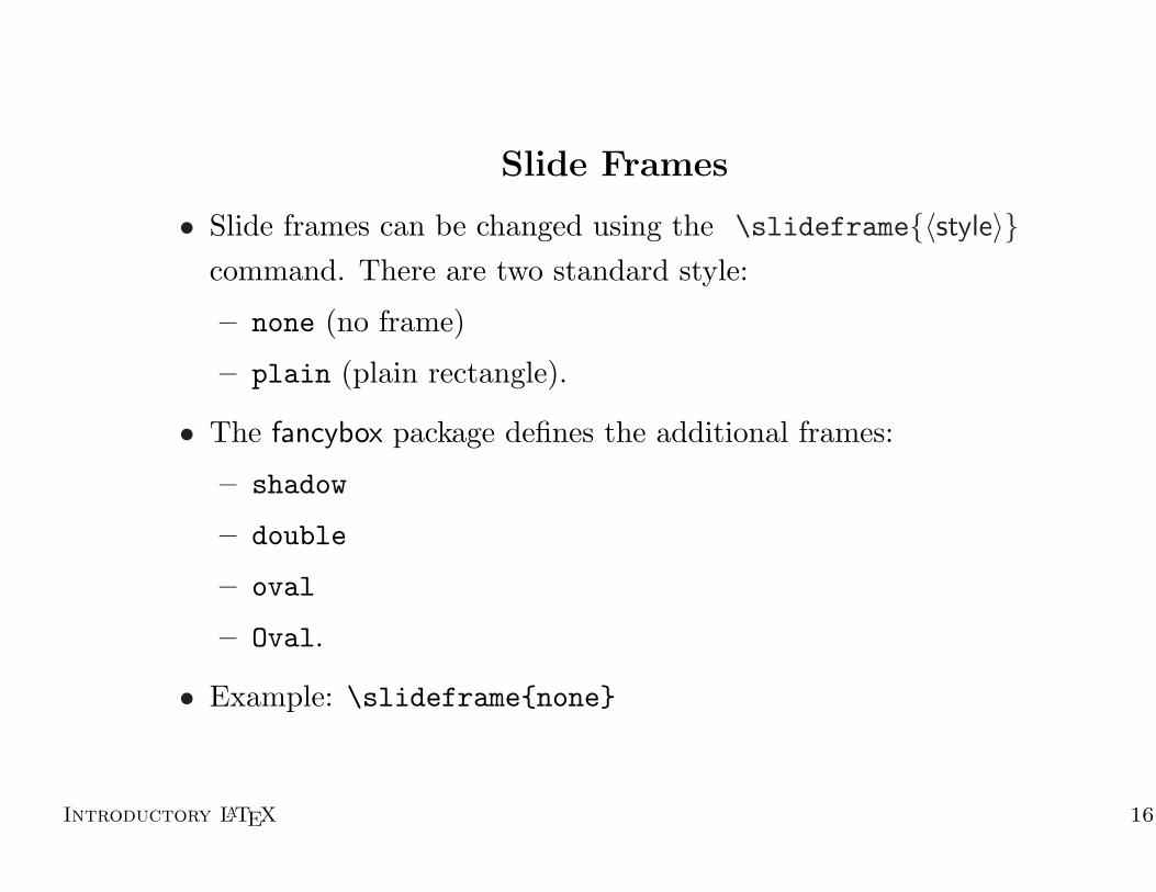
Slide Frames
• Slide frames can be changed using the \slideframe{〈style〉}command. There are two standard styles:
– none (no frame)
– plain (plain rectangle).
• The fancybox package defines the additional styles:
– shadow
– double
– oval
– Oval.
• Example: \slideframe{plain}
Introductory LATEX 160
Slide Frames
• Slide frames can be changed using the \slideframe{〈style〉}command. There are two standard style:
– none (no frame)
– plain (plain rectangle).
• The fancybox package defines the additional frames:
– shadow
– double
– oval
– Oval.
• Example: \slideframe{none}
Introductory LATEX 161

'
&
$
%
Slide Frames
• Slide frames can be changed using the \slideframe{〈style〉}command. There are two standard style:
– none (no frame)
– plain (plain rectangle).
• The fancybox package defines the additional frames:
– shadow
– double
– oval
– Oval.
• Example: \slideframe{Oval}
Introductory LATEX 162

Slide Frames
• Slide frames can be changed using the \slideframe{〈style〉}command. There are two standard style:
– none (no frame)
– plain (plain rectangle).
• The fancybox package defines the additional frames:
– shadow
– double
– oval
– Oval.
• Example: \slideframe{shadow}
Introductory LATEX 163

Slide Frames
• Slide frames can be changed using the \slideframe{〈style〉}command. There are two standard style:
– none (no frame)
– plain (plain rectangle).
• The fancybox package defines the additional frames:
– shadow
– double
– oval
– Oval.
• Example: \slideframe{double}
Introductory LATEX 164

Colour
• Use color or pstcol package.
\usepackage[usenames]{pstcol}
• Page colour is set using \pagecolor{〈colour〉}\pagecolor{Blue}
• Text colour can be set using:
– \color{〈colour〉} (declaration)
\color{Yellow}
– \textcolor{〈colour〉}{〈text〉}\textcolor{Green}{Some green text}
Introductory LATEX 165

Customising Slide Frames using PostScript
• It is possible to design more interesting slide frames usingPostScript. See the LATEX Graphics Companion for more details.
• The seminar class file allows new page styles to be defined usingthe command:
\newpagestyle{〈name〉}{〈header〉}{〈footer〉}
\newpagestyle{csedlatex}{}{%
\textsc{Introductory \LaTeX}\hfill\thepage}
\pagestyle{csedlatex}
Introductory LATEX 166

Exercise 20 (Page 35)
• Try to produce some of the slides used during this course.
• Try experimenting with different slide frames, and different pagestyles.
• Try including some notes about the slides.
• Try using the article option.
• With the article option, the slide caption is displayed accordingto the style specified by the command \slidestyle{〈style〉} .Available options are: empty, left, bottom. Try experimentingwith the slide style.
Introductory LATEX 167

Defining New Environments
New environments can be defined using:
\newenvironment{〈env-name〉}[〈n〉][〈default〉]{〈begin-code〉}{〈end-code〉}
\newenvironment{bfitemize}%
{\begin{bfseries}\begin{itemize}}%
{\end{itemize}\end{bfseries}}
\begin{bfitemize}
\item First item
\item Second item
\end{bfitemize}
Input
� First item
� Second item
Output
Introductory LATEX 168

Example Environment with Argument
\newsavebox{\fminibox}
\newenvironment{fminipage}[2][c]%
{\begin{lrbox}{\fminibox}\begin{minipage}[#1]{#2}}%
{\end{minipage}\end{lrbox}%
\shadowbox{\usebox{\fminibox}}}
Input
\begin{fminipage}{1.5in}
Some text in a 1.5
inch framed minipage
\end{fminipage}
Input
Some text in a 1.5 inch
framed minipage
Output
Introductory LATEX 169
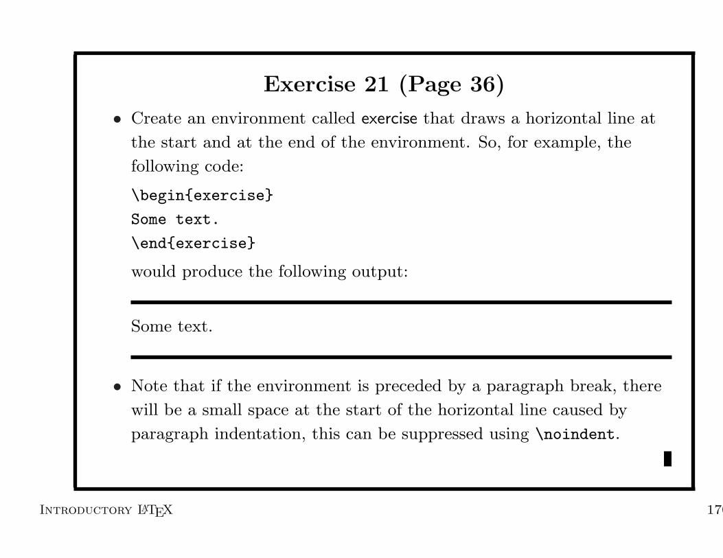
Exercise 21 (Page 36)
• Create an environment called exercise that draws a horizontal line at
the start and at the end of the environment. So, for example, the
following code:
\begin{exercise}
Some text.
\end{exercise}
would produce the following output:
Some text.
• Note that if the environment is preceded by a paragraph break, there
will be a small space at the start of the horizontal line caused by
paragraph indentation, this can be suppressed using \noindent.
Introductory LATEX 170

Counters
• Counters contain integers that can be incremented ordecremented.
• To define a new counter:
\newcounter{〈ctr-name〉}[〈outer-ctr〉]For example: \newcounter{exercise}.
• To reset the counter every time another counter is incremented:\newcounter{exercise}[chapter]
Introductory LATEX 171

Changing the Value of a Counter
• \stepcounter{〈ctr〉} increment the counter
• \refstepcounter{〈ctr〉} as above, but allows you to referencethe counter using \ref and \label.
• \setcounter{〈ctr〉}{〈value〉} set the counter to 〈value〉
• \addtocounter{〈ctr〉}{〈value〉} add 〈value〉 to the counter
• \value{〈ctr〉} This command produces the value for use in the
〈value〉 part of \setcounter and \addtocounter commands.
Introductory LATEX 172

Displaying the Value of a Counter
• The command \the〈ctr〉 prints a representation of the value associated
with 〈ctr〉.
• \arabic{〈ctr〉} print 〈ctr〉 as an arabic numeral
• \roman{〈ctr〉} print 〈ctr〉 as a lowercase roman numeral
• \Roman{〈ctr〉} print 〈ctr〉 as an uppercase Roman numeral
• \alph{〈ctr〉} print 〈ctr〉 as a lowercase letter (value of counter must be less
than 26)
• \Alph{〈ctr〉} print 〈ctr〉 as an uppercase letter (value of counter must be
less than 26)
• \fnsymbol{〈ctr〉} print 〈ctr〉 as a footnote symbol. (This command may
only be used in maths mode)
Introductory LATEX 173

Examples
• \thechaper displays the value of the chapter counter.
• \renewcommand{\thechapter}{\Roman{chapter}} redefines\thechapter so that it displays the chapter number as anuppercase Roman numeral.
• \renewcommand{\thefootnote}{\alph{footnote}} will displaythe footnote counter as a lowercase letter
• \newcounter{lemma}[section] defines a new counter calledlemma that will be reset at the start of each section.
• \renewcommand{\thelemma}{\thesection.\arabic{lemma}} Ifthe section number is 4 and the lemma number is 3, \thelemmawill display 4.3
Introductory LATEX 174

Other ways of displaying the value of a counter
The datetime package also provides the following commands fordisplaying the value of a counter:
\ordinal{〈counter〉} Display the value of 〈counter〉 as anordinal
\ordinalstring{〈counter〉} Display the value of 〈counter〉 as anordinal written out in full
\Ordinalstring{〈counter〉} As above, but with the initial let-ters in uppercase
\numberstring{〈counter〉} Display the value of 〈counter〉 as astring
\Numberstring{〈counter〉} As above but with the initial letterin uppercase
Introductory LATEX 175

Examples
\ordinal{slide}
Input
176th
Output
\ordinalstring{slide}
Input
one hundred and seventy-sixth
Output
\Ordinalstring{slide}
Input
One Hundred and Seventy-Sixth
Output
\numberstring{slide}
Input
one hundred and seventy-six
Output
\Numberstring{slide}
Input
One Hundred and Seventy-Six
Output
Introductory LATEX 176

Enumeration Counters
Up to four nested enumerate environments are permitted. Each levelhas an associated counter:
Counter Representation Default Example
enumi \theenumi \arabic{enumi} 1
\labelenumi \theenumi. 1.
enumii \theenumii \alph{enumii} a
\labelenumii \theenumii) a)
enumiii \theenumiii \roman{enumiii} i
\labelenumiii \theenumiii. i.
enumiv \theenumiv \Alph{enumiv} A
\labelenumiv \theenumiv. A.
Introductory LATEX 177

Changing enumerate Counter Format
\renewcommand{\theenumi}{\Roman{enumi}}
Input
\begin{enumerate}
\item\label{itm:first} First item
\item Second item
\end{enumerate}
Item~\ref{itm:first} \ldots
Input
I. First item
II. Second item
Item I . . .
Output
Introductory LATEX 178

Changing enumerate Label
\renewcommand{\labelenumi}{\#\theenumi}
Input
\begin{enumerate}
\item\label{itm:first} First item
\item Second item
\end{enumerate}
Item~\ref{itm:first} \ldots
Input
#1 First item
#2 Second item
Item 1 . . .
Output
Introductory LATEX 179

Changing enumerate Format
\renewcommand{\theenumi}{\Numberstring{enumi}}
\renewcommand{\labelenumi}{\theenumi:}
Input
\begin{enumerate}
\item\label{itm:first} First item
\item Second item
\end{enumerate}
Item~\ref{itm:first} \ldots
Input
One: First item
Two: Second item
Item One . . .
Output
Introductory LATEX 180

Exercise 22 (Page 38)
• Modify the environment you created in Exercise 21 so that for
example, the following code:
\begin{exercise}
Some text.
\end{exercise}
would produce the following output:
Exercise 1Some text.
• The value of the counter will need to be incremented at the start of
each exercise.
• Try referencing it using \label and \ref.
Introductory LATEX 181

Web Sites
• TEX archive site:
http://www.tex.ac.uk/
• These slides are available at:
http://theoval.sys.uea.ac.uk/~gcc/family/nicky/latex/csed.html
Introductory LATEX 182