Embed Size (px)
Citation preview

Introductory Examples for
System Identification
Munther A. Dahleh
Lecture 2 6.435, System Identification Prof. Munther A. Dahleh
1
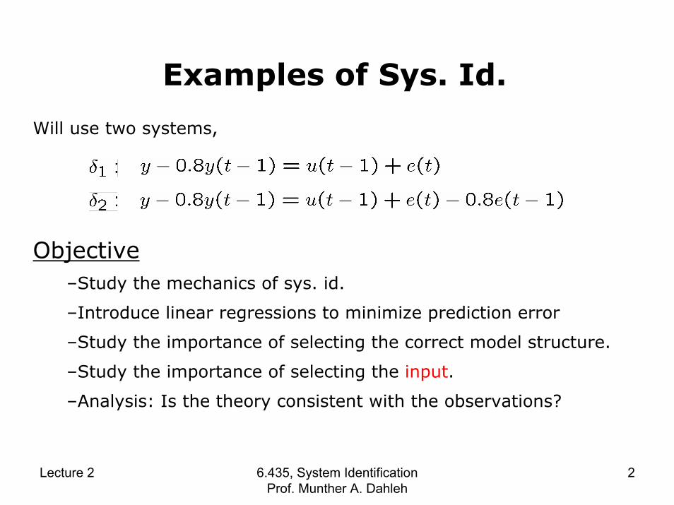
Examples of Sys. Id.
Will use two systems,
Objective–Study the mechanics of sys. id.
–Introduce linear regressions to minimize prediction error
–Study the importance of selecting the correct model structure.
–Study the importance of selecting the input.
–Analysis: Is the theory consistent with the observations?
Lecture 2 6.435, System Identification Prof. Munther A. Dahleh
2
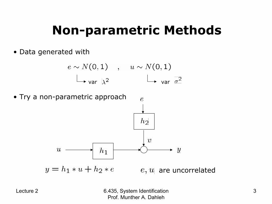
Non-parametric Methods
• Data generated with
var var
• Try a non-parametric approach
are uncorrelated
Lecture 2 6.435, System Identification Prof. Munther A. Dahleh
3

• One way of recovering is to correlate the data with and thus get rid of the noise.
• Method called: Correlation analysis
• Note: If are uncorrelated , then
are uncorrelated
• The method does not estimate .
Lecture 2 6.435, System Identification Prof. Munther A. Dahleh
4

Correlation Analysis
•
• Compute exactly.
•
• Approximation: Ergodicity assumptions.
• The Frequency response
• Comparisons!
Lecture 2 6.435, System Identification Prof. Munther A. Dahleh
5

actualspa
Lecture 2 6.435, System Identification Prof. Munther A. Dahleh
6
actualspa
Lecture 2 6.435, System Identification Prof. Munther A. Dahleh
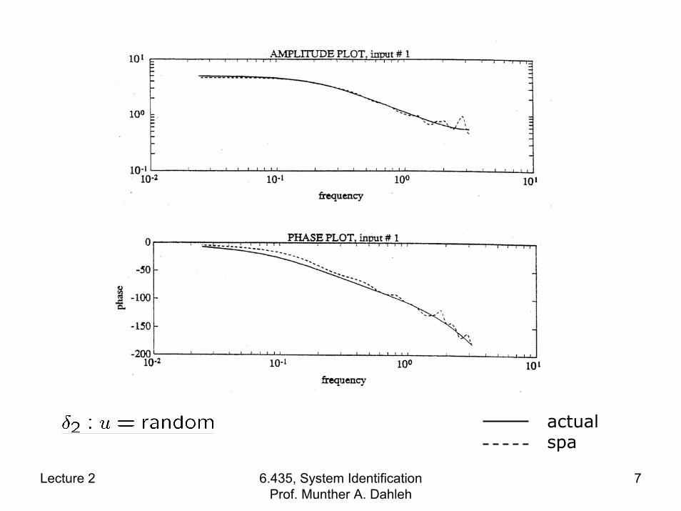
7

Comments
• Both systems have a “fairly” good low-freq approximation.
• For system 1, there is an error in the low frequency range.
•
noise for is amplified in the low frequency range.
Lecture 2 6.435, System Identification Prof. Munther A. Dahleh
8
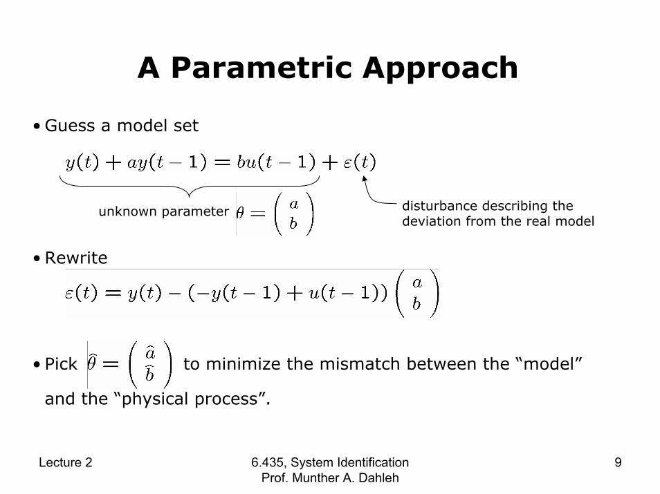
A Parametric Approach
• Guess a model set
disturbance describing the deviation from the real model
unknown parameter
• Rewrite
• Pick to minimize the mismatch between the “model”
and the “physical process”.
Lecture 2 6.435, System Identification Prof. Munther A. Dahleh
9

• Define
• Estimate at time , is given by:
Lecture 2 6.435, System Identification Prof. Munther A. Dahleh
10

Calculation of
• Expand in a matrix form
•
Lecture 2 6.435, System Identification Prof. Munther A. Dahleh
11

•
(see 6.241)
pseudo-inverse
•
all •
Lecture 2 6.435, System Identification Prof. Munther A. Dahleh
12
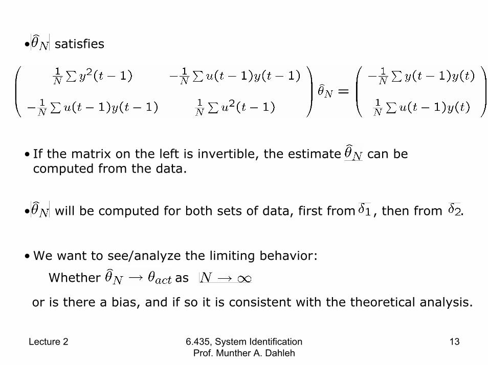
• satisfies
• If the matrix on the left is invertible, the estimate can be computed from the data.
• will be computed for both sets of data, first from , then from .
• We want to see/analyze the limiting behavior:
Whether as
or is there a bias, and if so it is consistent with the theoretical analysis.
Lecture 2 6.435, System Identification Prof. Munther A. Dahleh
13
Simulations
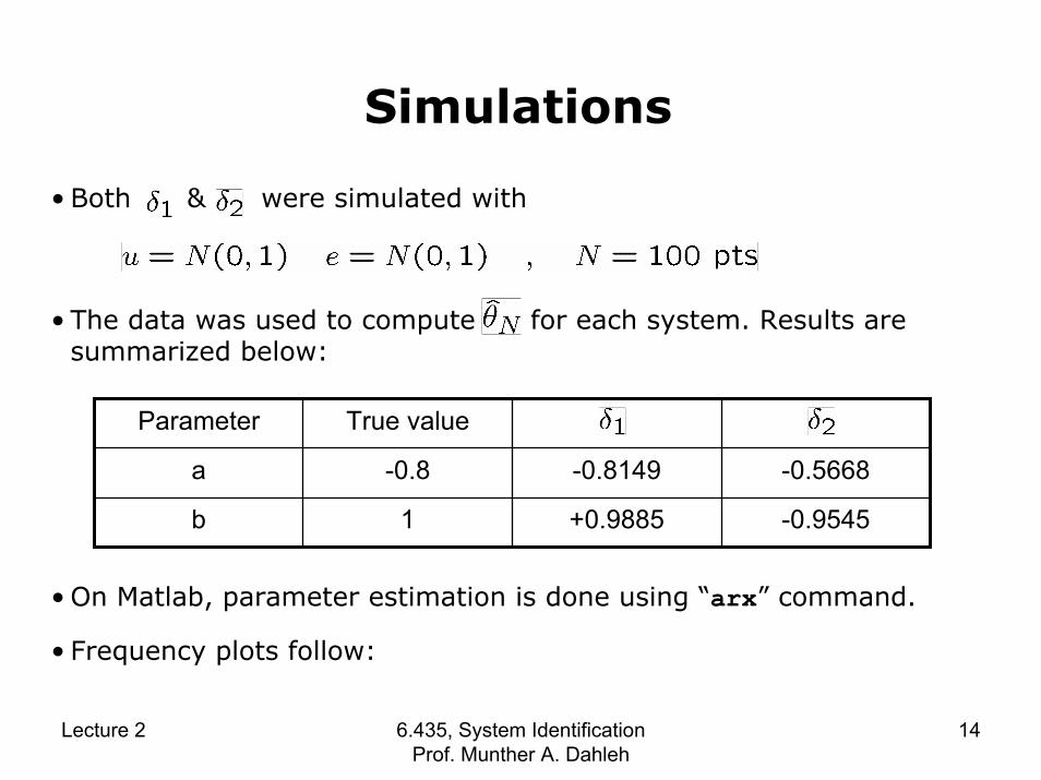
• Both & were simulated with
• The data was used to compute for each system. Results are summarized below:
Parameter True value
a -0.8 -0.8149 -0.5668
b 1 +0.9885 -0.9545
• On Matlab, parameter estimation is done using “arx” command.
• Frequency plots follow:
Lecture 2 6.435, System Identification Prof. Munther A. Dahleh
14

actualarx
Lecture 2 6.435, System Identification Prof. Munther A. Dahleh
15
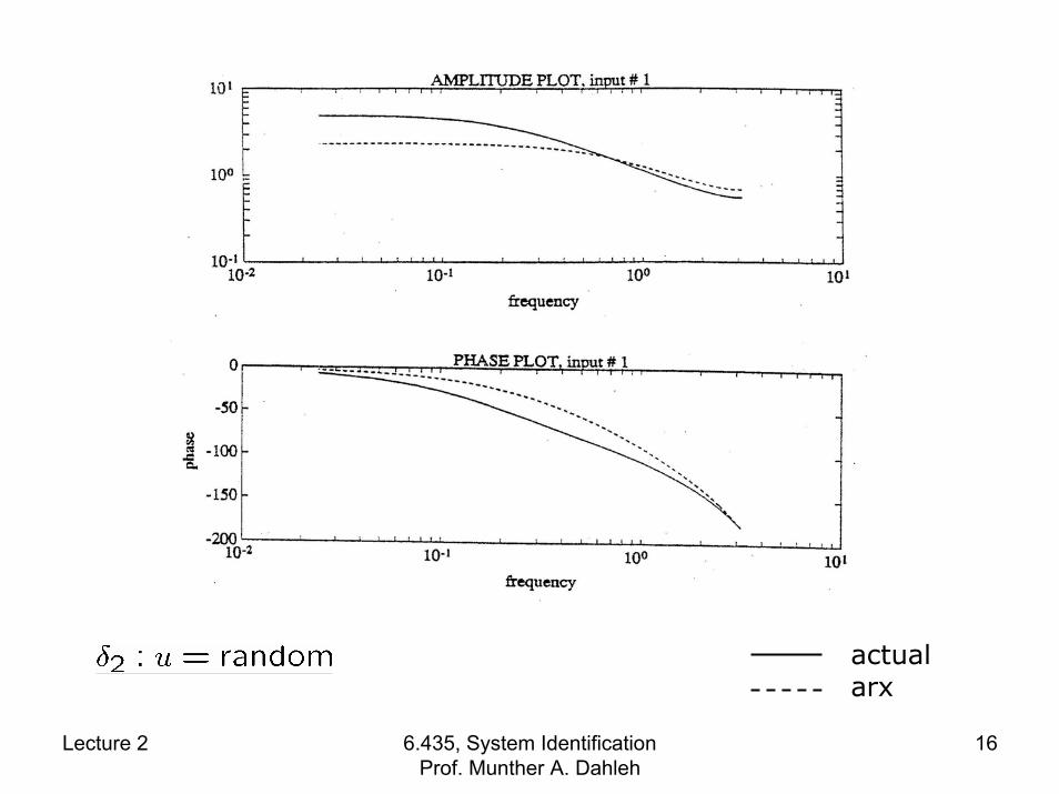
actualarx
Lecture 2 6.435, System Identification Prof. Munther A. Dahleh
16

Comments
• For System I, the model structure is identical to the model of the processes. Thus, the parameters converged to the real parameters.
• For System II, the model structure is different from the actual model. The estimated parameters had a bias.
• Is this consistent with the theoretical analysis? Are the numbers that we got meaningful or is it possible that a different simulation can yield drastically different estimated parameters?
• Theoretical analysis will explain the observations.
Lecture 2 6.435, System Identification Prof. Munther A. Dahleh
17
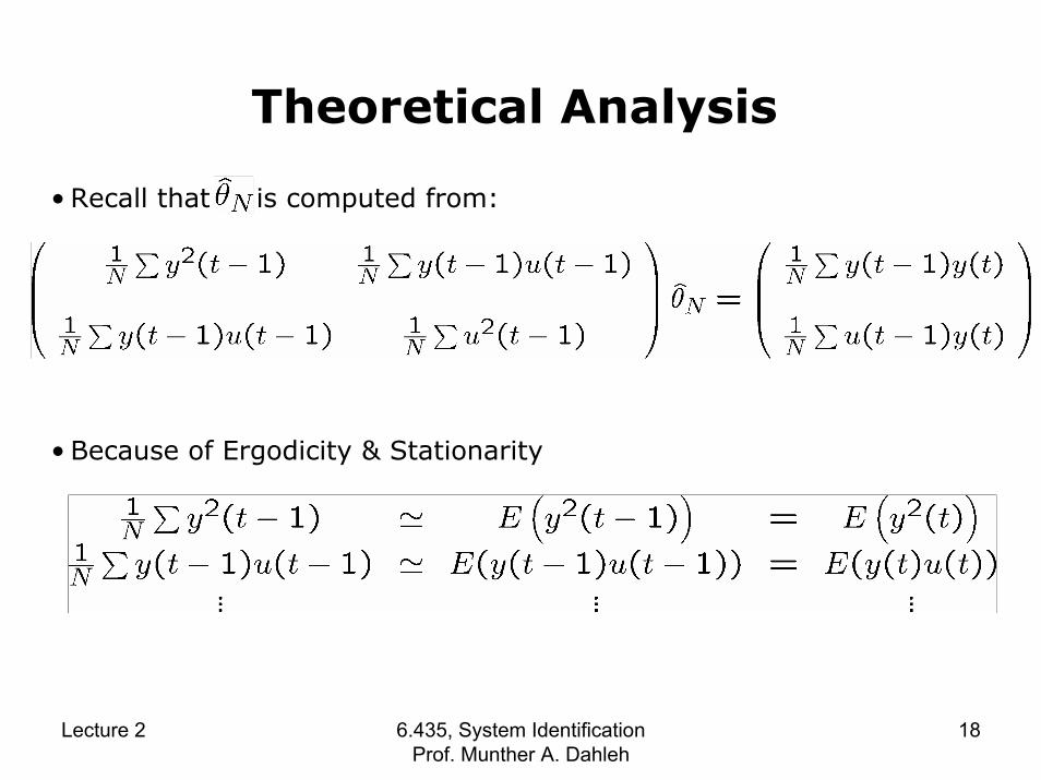
Theoretical Analysis
• Recall that is computed from:
• Because of Ergodicity & Stationarity
Lecture 2 6.435, System Identification Prof. Munther A. Dahleh
18
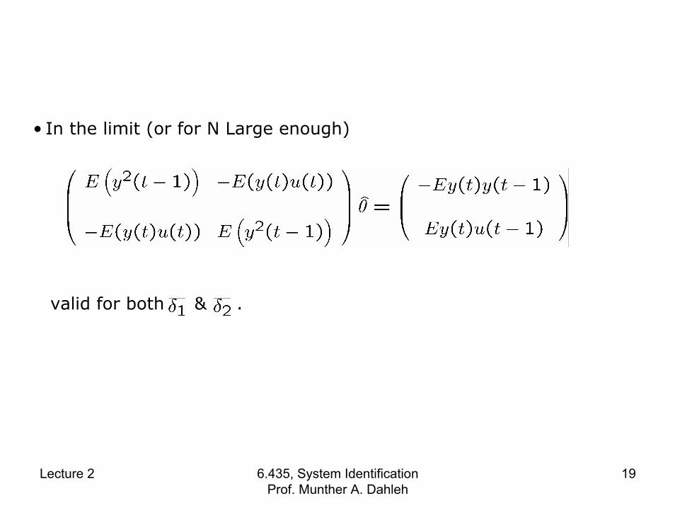
• In the limit (or for N Large enough)
valid for both & .
Lecture 2 6.435, System Identification Prof. Munther A. Dahleh
19

The General Case
are uncorrelated
• Compute
=0 =0
=0 =0 =0
Lecture 2 6.435, System Identification Prof. Munther A. Dahleh
20

•
•=0 =0
Lecture 2 6.435, System Identification Prof. Munther A. Dahleh
21

•
• Compute the estimate in the general case:
Lecture 2 6.435, System Identification Prof. Munther A. Dahleh
22
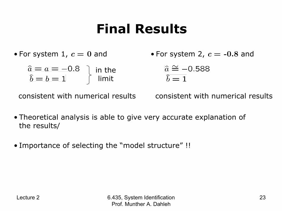
Final Results
• For system 1, c = 0 and • For system 2, c = -0.8 and
in the limit
consistent with numerical results consistent with numerical results
• Theoretical analysis is able to give very accurate explanation of the results/
• Importance of selecting the “model structure” !!
Lecture 2 6.435, System Identification Prof. Munther A. Dahleh
23
Experiment Design
• All the previous results were based on data generated white Gaussian. (In fact, the signals are called PRBS, pseudo-random binary sequence). Such inputs are quite rich.
• How about using an input which is not very rich
e.g. a step input
• Observe
– Non-parametric results
– Parametric results
– Theoretical analysis
Lecture 2 6.435, System Identification Prof. Munther A. Dahleh
24

Step Input
• & were simulated with
step
• Results from the parameter estimation are given below:
Parameter True value
a -0.8 -0.72 0.0136
b 1 1.377 5.0324
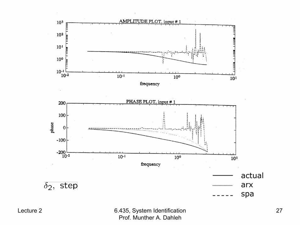
• Frequency plots follow for the actual system, the parametric estimated system, and the nonparametric estimate (based on correlation / freq methods).
Lecture 2 6.435, System Identification Prof. Munther A. Dahleh
25

actualarxspa
Lecture 2 6.435, System Identification Prof. Munther A. Dahleh
26
actualarxspa
Lecture 2 6.435, System Identification Prof. Munther A. Dahleh
27
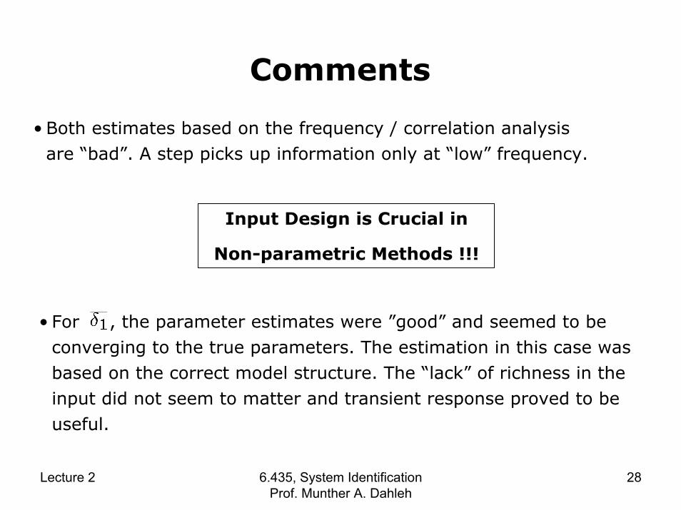
Comments
• Both estimates based on the frequency / correlation analysis are “bad”. A step picks up information only at “low” frequency.
Input Design is Crucial in
Non-parametric Methods !!!
• For , the parameter estimates were ”good” and seemed to be converging to the true parameters. The estimation in this case was based on the correct model structure. The “lack” of richness in the input did not seem to matter and transient response proved to beuseful.
Lecture 2 6.435, System Identification Prof. Munther A. Dahleh
28

• For , the parameters were “way off”, and the frequency plot is quite bad.
Lack of richness + incorrect model structure ⇒ bad results
• Question: Are these results dependent on the simulations? If not, can they be analyzed theoretically?
• We will show that the theoretical analysis will in fact predict this behavior.
Lecture 2 6.435, System Identification Prof. Munther A. Dahleh
29

Theoretical Analysis
• Recall
for deterministic signals.• Remember
step, with amplitude .
• In general
need to compute all the quantities:
Lecture 2 6.435, System Identification Prof. Munther A. Dahleh
30
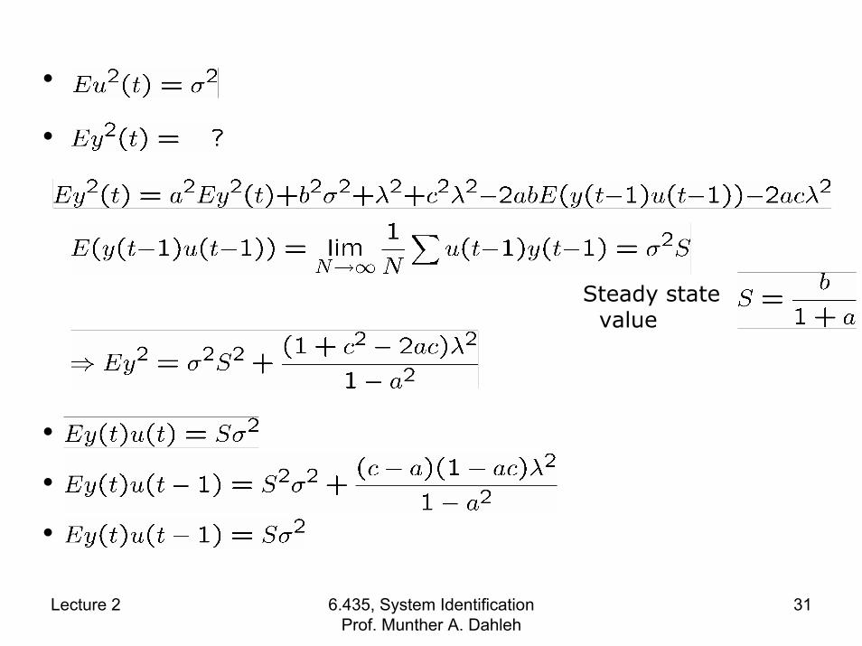
•
•
Steady state value
•
•
•
Lecture 2 6.435, System Identification Prof. Munther A. Dahleh
31

• The estimates
• For , c = 0 and
consistent with numerical results
• For , c = -0.8 and
consistent with numerical results
– Note that the s.s gain is correctly estimated.
• Complete agreement. Results are independent of the calculations!
Lecture 2 6.435, System Identification Prof. Munther A. Dahleh
32
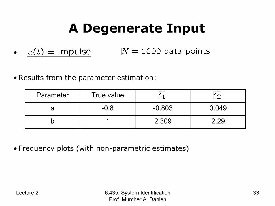
A Degenerate Input
•
• Results from the parameter estimation:
Parameter True value
a -0.8 -0.803 0.049
b 1 2.309 2.29
• Frequency plots (with non-parametric estimates)
Lecture 2 6.435, System Identification Prof. Munther A. Dahleh
33
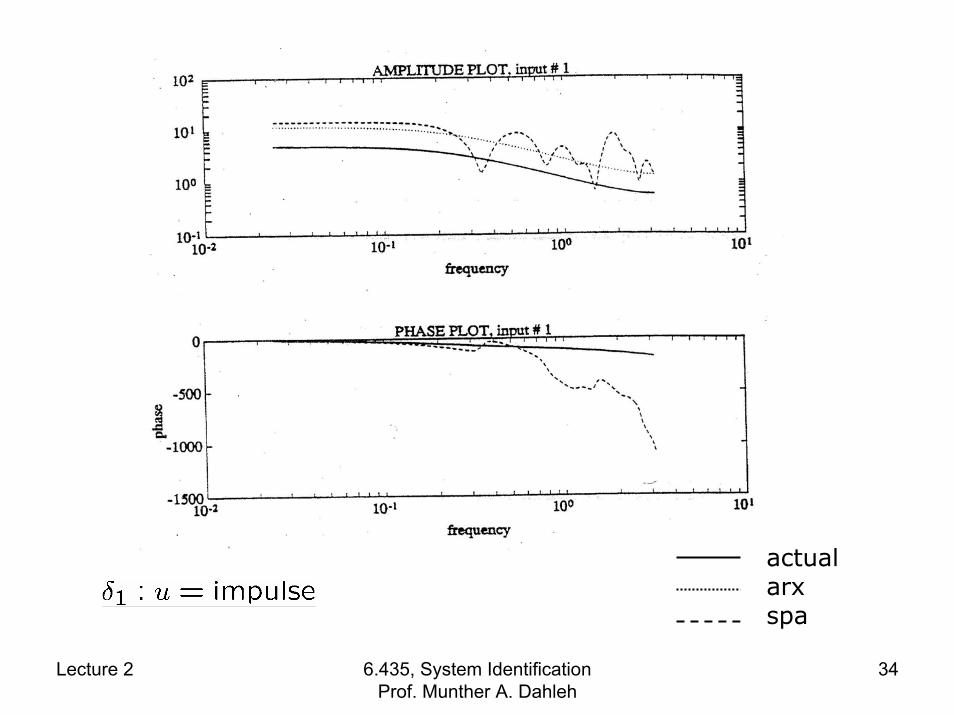
actualarxspa
Lecture 2 6.435, System Identification Prof. Munther A. Dahleh
34

actualarxspa
Lecture 2 6.435, System Identification Prof. Munther A. Dahleh
35
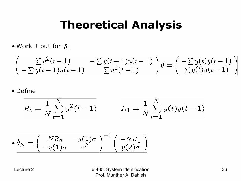
Theoretical Analysis
• Work it out for
• Define
•
Lecture 2 6.435, System Identification Prof. Munther A. Dahleh
36

• As and
• The estimates
Lecture 2 6.435, System Identification Prof. Munther A. Dahleh
37

Comments
• is estimated accurately,
depends on the particular sample function for e, in particular .
• Different simulations yield different results !!
• Get better results if σ is very large.
• Impulse is not a rich input!
Lecture 2 6.435, System Identification Prof. Munther A. Dahleh
38