Cosmology

V.A. RubakovInstitute for Nuclear Research of the Russian Academy of Sciences, Moscow, Russia

AbstractIn these lectures we first concentrate on the cosmological problems which,hopefully, have to do with the new physics to be probed at the LHC: the natureand origin of dark matter and generation of matter-antimatter asymmetry. Wegive several examples showing the LHC cosmological potential. These areWIMPs as cold dark matter, gravitinos as warm dark matter, and electroweakbaryogenesis as a mechanism for generating matter-antimatter asymmetry. Inthe remaining part of the lectures we discuss the cosmological perturbationsas a tool for studying the epoch preceeding the conventional hot stage of thecosmological evolution.

1 IntroductionThe more we learn about our Universe, the better we understand that it is full of mysteries. These fallinto three broad classes. One major mystery is dark energy, which deserves a separate class. We brieflydiscuss dark energy in Section 5, although, honestly speaking, we do not have much to say about it. Thesecond class most likely has to do with the early hot epoch of the cosmological evolution, and the thirdone with an even earlier stage which preceeded the hot epoch. Along with dark energy, we encountermysteries of the second class when studying the present composition of the Universe. It hosts matterbut not antimatter, and after 40 years after it was understood that this is a problem, we do not have anestablished theory explaining this asymmetry. The Universe hosts dark matter, and we do not know whatit is made of. In this context, one of the key players is the Large Hadron Collider. Optimistically, the LHCexperiments may discover dark matter particles and their companions, and establish physics behind thematter-antimatter asymmetry. Otherwise they will rule out some very plausible scenarios; this will alsohave profound impact on our understanding of the early Universe. Let us mention also exotic hypotheseson physics beyond the Standard Model, like TeV scale gravity; their support by the LHC will have aneffect on the early cosmology, which is hard to overestimate.

In the first part of these lectures we concentrate on a few examples showing the LHC cosmologicalpotential. Before coming to that, we briefly introduce the basic notions of cosmology that are useful forour main discussion. We then turn to dark matter, and present the WIMP scenario for cold dark matter,which is currently the most popular one — for good reason. We also consider light gravitino scenariofor warm dark matter. Both are probed by the LHC, as they require rather particular new physics inthe LHC energy range. We then discuss electroweak baryogenesis — a mechanism for the generationof matter-antimatter asymmetry that may have operated at temperature of order 100 GeV in the earlyUniverse. This mechanism also needs new physics at energies 100− 300 GeV, so it will be confirmed orruled out by the LHC.

The third class of mysteries is related to cosmological perturbations, i.e., inhomogeneities in en-ergy density and associated gravitational potentials and, possibly, relic gravity waves. As we explain inthe second part of these lectures, the observed properties of density perturbations show that they weregenerated at some epoch that preceeded the hot stage of the cosmological evolution. Obviously, the veryfact that we are confident about the existence of such an epoch is a fundamental result of theoretical andobservational cosmology. The most plausible hypothesis on that epoch is cosmological inflation, thoughthe observational support of this hypothesis is presently not particularly strong, and alternative scenarioshave not been ruled out. We will briefly discuss the potential of future cosmological observations indiscriminating between different options.

arX

iv:1

504.

0358

7v1

[as

tro-

ph.C

O]

14

Apr

201

5

These lectures are meant to be self-contained, but we necessarily omit numerous details, whiletrying to make clear the basic ideas and results. More complete accounts of particle physics aspects ofcosmology may be found in reviews [1]. Dark matter, including various hypotheses about its particles,is reviewed in Ref. [2]. Electroweak baryogenesis is discussed in detail in reviews [3]. For reviews ondark energy, see, e.g., Ref. [4]. The theory and observations of cosmological perturbations are presentedin Ref. [5].

2 Homogeneous isotropic Universe2.1 Friedmann–Lemaître–Robertson–Walker metricTwo basic facts about our visible Universe are that it is homogeneous and isotropic at large spatial scales,and that it expands.

There are three types of homogeneous and isotropic three-dimensional spaces. These are1 three-sphere, flat (Euclidean) space and three-hyperboloid. Accordingly, one speaks about closed, flat andopen Universe; in the latter two cases the spatial size of the Universe is infinite, whereas in the formerthe Universe is compact.

The homogeneity and isotropy of the Universe mean that its hypersurfaces of constant time areeither three-spheres or Euclidean spaces or three-hyperboloids. The distances between points may (and,indeed, do) depend on time, i.e., the interval has the form

ds2 = dt2 − a2(t)dx2 , (1)

where dx2 is the distance on unit three-sphere/Euclidean space/hyperboloid. The metric (1) is usuallycalled Friedmann–Lemaître–Robertson–Walker (FLRW) metric, and a(t) is called the scale factor. Inour Universe a ≡ da

dt > 0, which means that the distance between points of fixed spatial coordinates xgrows, dl2 = a2(t)dx2. The space stretches out; the Universe expands.

The coordinates x are often called comoving coordinates. It is straightforward to check that x =const is a time-like geodesic, so a galaxy put at a certain x at zero velocity will stay at the same x.Furthermore, as the Universe expands, non-relativistic objects loose their velocities x, i.e., they getfrozen in the comoving coordinate frame.

Observational data set strong constraints on the spatial curvature of the Universe. They tell that toa very good approximation our Universe is spatially flat, i.e., our 3-dimensional space is Euclidean. Inwhat follows dx2 is simply the line interval in the Euclidean 3-dimensional space.

2.2 RedshiftLike the distances between free particles in the expanding Universe, the photon wavelength increasestoo. We will always label the present values of time-dependent quantities by subscript 0: the presentwavelength of a photon is thus denoted by λ0, the present time is t0, the present value of the scale factoris a0 ≡ a(t0), etc. If a photon was emitted at some moment of time t in the past, and its wavelength atthe moment of emission was λe, then we receive today a photon whose physical wavelength is longer,

λ0

λe=

a0

a(t)≡ 1 + z .

Here we introduced the redshift z. The redshift of an object is directly measurable. λe is fixed byphysics of the source, say, it is the wavelength of a photon emitted by an excited hydrogen atom. So,

1Strictly speaking, this statement is valid only locally: in principle, homogeneous and isotropic Universe may have complexglobal properties. As an example, spatially flat Universe may have topology of three-torus. There is some discussion ofsuch a possibility in literature, and fairly strong limits have been obtained by the analyses of cosmic microwave backgroundradiation [6].

2

one identifies a series of emission or absorption lines, thus determining λe, and measures their actualwavelengths λ0. These spectroscopic measurements give accurate values of z even for distant sources.On the other hand, the redshift is related to the time of emission, and hence to the distance to the source.

Let us consider a “nearby” source, for which z 1. This corresponds to relatively small (t0− t).Expanding a(t), one writes

a(t) = a0 − a(t0)(t0 − t) . (2)

To the leading order in z, the difference between the present time and the emission time is equal to thedistance to the source r (the speed of light is set equal to 1). Let us define the Hubble parameter

H(t) =a(t)

a(t)

and denote its present value by H0. Then Eq. (2) takes the form a(t) = a0(1−H0r), and we get for theredshift, again to the leading non-trivial order in z,

1 + z =1

1−H0r= 1 +H0r .

In this way we obtain the Hubble law,

z = H0r , z 1 . (3)

Traditionally, one tends to interpret the expansion of the Universe as runaway of galaxies from eachother, and redshift as the Doppler effect. Then at small z one writes z = v, where v is the radial velocityof the source with respect to the Earth, so H0 is traditionally measured in units “velocity per distance”.Observational data give [8]

H0 = [71.0± 2.5]km/sMpc

≈ (14 · 109 yrs)−1 , (4)

where 1 Mpc = 3 · 106 light yrs = 3 · 1024 cm is the distance measure often used in cosmology.Traditionally, the present value of the Hubble parameter is written as

H0 = h · 100km

s ·Mpc. (5)

Thus h ≈ 0.71. We will use this value in further estimates.

Let us point out that the interpretation of redshift in terms of the Doppler shift is actually notadequate, especially for large enough z. In fact, there is no need in this interpretation at all: the “ra-dial velocity” enters neither theory nor observations, so this notion may be safely dropped. Physicallymeaningful quantity is redshift z itself.

A final comment is that H−10 has dimension of time, or length, as indicated in Eq. (4). Clearly,

this quantity sets the cosmological scales of time and distance at the present epoch.

2.3 Hot UniverseOur Universe is filled with cosmic microwave background (CMB). Cosmic microwave background asobserved today consists of photons with excellent black-body spectrum of temperature

T0 = 2.726± 0.001 K . (6)

The spectrum has been precisely measured by various instruments and does not show any deviation fromthe Planck spectrum [7].

3

Thus, the present Universe is “warm”. Earlier Universe was warmer; it cooled down because ofthe expansion. While the CMB photons freely propagate today, it was not so at early stage. When theUniverse was hot, the usual matter (electrons and protons with rather small admixture of light nuclei)was in the plasma phase. At that time photons strongly interacted with electrons due to the Thomsonscattering and protons interacted with electrons via Coulomb force, so all these particles were in thermalequilibrium. As the Universe cooled down, electrons “recombined” with protons into neutral hydrogenatoms, and the Universe became transparent to photons. The temperature scale of recombination is, verycrudely speaking, determined by the ionisation energy of hydrogen, which is of order 10 eV. In fact,recombination occured at lower temperature2, Trec ≈ 3000 K. An important point is that the duration ofthe period of recombination was considerably shorter than the Hubble time at that epoch; to a reasonableapproximation, recombination occured instantaneously.

The importance of the recombination epoch (more precisely, the epoch of photon last scattering;we will use the term recombination for brevity) is that the CMB photons travel freely after it: the densityof hydrogen atoms was so small (about 250 cm−3 right after recombination) that the gas was transparentto photons. So, CMB photons give the photographic picture of the Universe at recombination, i.e., atredshift and age

zrec = 1090 , trec = 370 000 years . (7)

It is worth noting that even though after recombination photons no longer were in thermal equi-librium with anything, the shape of the photon distribution function has not changed, except for overallredshift. Indeed, the thermal distribution function for ultra-relativistic particles, the Planck distribution,depends only on the ratio of frequency to temperature, fPlanck(p, T ) = f (ωp/T ), ωp = |p|. As the Uni-verse expands, the photon momentum gets redshifted, p(t) = p(trec) · a(trec)

a(t) , the frequency is redshiftedin the same way, but the shape of the spectrum remains Planckian, with redshifted temperature. Hence,the Planckian form of the observed spectrum is no surprise. Generaly speaking, this property does nothold for massive particles.

At even earlier times, the temperature of the Universe was even higher. The earliest time at the hotstage which has been observationally probed so far is the Big Bang Nucleosynthesis epoch; that epochbegan at temperature of order 1 MeV, when the lifetime of the Universe was about 1 s. At that time theweak processes like

e− + p←→ n+ νe

switched off, and the comoving number density of neutrons freezed out. Somewhat later, these neutronscombined with protons into light elements in thermonuclear reactions

p+ n → 2H + γ ,2H + p → 3He+ γ ,

3He+2 H → 4He+ p , (8)

etc., up to 7Li. Comparison of the Big Bang Nucleosynthesis theory with the observational determinationof the composition of cosmic medium gives us confidence that we understand the Universe at that epoch.Notably, we are convinced that the cosmological expansion was governed by General Relativity.

2.4 Properties of components of cosmic mediumLet us come back to photons. Their effective temperature after recombination scales as

T (t) ∝ a−1(t) . (9)2The reason is that the number density of electrons and protons is small compared to the number density of photons. At

temperature above 3000 K, a hydrogen atom formed in an electron-proton encounter is quickly destroyed by absorbing aphoton from the high energy tail of the Planck distribution, and after that the electron/proton lives long time before it meetsproton/electron and forms a hydrogen atom again. In thermodynamical terms, at temperatures above 3000 K there is largeentropy per electron/proton, and recombination is not thermodynamically favourable because of entropy considerations.

4

This behaviour is characteristic of ultra-relativistic free species (at zero chemical potential). The sameformula is valid for ultra-relativistic particles (at zero chemical potential) which are in thermal equilib-rium. Thermal equilibrium means adiabatic expansion; during adiabatic expansion, the temperature ofultra-relativistic gas scales as the inverse size of the system, according to usual thermodynamics. Theenergy density of ultra-relativistic gas scales as ρ ∝ T 4, and pressure is p = ρ/3.

Both for free photons, and for photons in thermal equilibrium, the number density behaves asfollows,

nγ = const · T 3 ∝ a−3 ,

and the energy density is given by the Stefan–Boltzmann law,

ργ =π2

30· 2 · T 4 ∝ a−4 , (10)

where the factor 2 accounts for two photon polarizations. The present number density of relic photons is

nγ,0 = 410 cm−3 , (11)

and their energy density is

ργ,0 = 2.7 · 10−10 GeVcm3

. (12)

An important characteristic of the early Universe is the entropy density of cosmic plasma in ther-mal equilibrium. It is given by

s =2π2

45g∗T 3 , (13)

where g∗ is the number of degrees of freedom with m . T , that is, the degrees of freedom which arerelativistic at temperature T ; each spin state counts as an independent degree of freedom, and fermionscontribute to g∗ with a factor of 7/8. The point is that the entropy density scales exactly as a−3,

sa3 = const , (14)

while temperature scales approximately as a−1. The property (14) is nothing but the reflection of the factthat the Universe expands relatively slowly, and the evolution is adiabatic (barrig fairly exotic scenarioswith strong entropy generation at some early cosmological epoch). The temperature would scale asa−1 if the number of relativistic degrees of freedom would be independent of time. This is not thecase, however. Indeed, the value of g∗ depends on temperature: at T ∼ 10 MeV relativistic speciesare photons, neutrinos, electrons and positrons, while at T ∼ 1 GeV four flavors of quarks, gluons,muons and τ -leptons are relativistic too. The number of degrees of freedom in the Standard Model atT & 100 GeV is

g∗(100 GeV) ≈ 100 .

The present value of the entropy density (taking into account neutrinos as if they were massless) is

s0 ≈ 3000 cm−3 . (15)

The parameter g∗ determines not only the entropy density but also the energy density of the cosmicplasma in thermal equilibrium. The Stefan–Boltzmann law gives

ρrad =π2

30g∗T 4 , (16)

where subscript rad indicates that we are talking about the relativistic component (radiation in broadsense).

5

Let us now turn to non-relativistic particles: baryons, massive neutrinos, dark matter particles,etc. If they are not destroyed during the evolution of the Universe (that is, they are stable and do notannihilate), their number density merely gets diluted,

n ∝ a−3 . (17)

This means, in particular, that the baryon-to-photon ratio stays constant in time (we consider for definite-ness the late Universe, T . 100 keV),

ηB ≡nBnγ

= const ≈ 6.1 · 10−10 . (18)

The numerical value here is determined by two independent methods: one is Big Bang Nucleosynthesistheory and measurements of the light element abundances, and another is the measurements of the CMBtemperature anisotropy. It is reassuring that these methods give consistent results (with comparableprecision).

The energy density of non-relativistic particles scales as

ρ(t) = m · n(t) ∝ a−3(t) , (19)

in contrast to more rapid fall off (10) characteristic of relativistic species.

Finally, dark energy density does not decrease in time as fast as in Eqs. (10) or (19). In fact, to areasonable approximation dark energy density does not depend on time at all,

ρΛ = const . (20)

Dark energy with exactly time-independent energy density is the same thing as the cosmological constant,or Λ-term.

2.5 Composition of the present UniverseThe basic equation governing the expansion rate of the Universe is the Friedmann equation, which wewrite for the case of spatially flat Universe,

H2 ≡(a

a

)2

=8π

3Gρ , (21)

where dot denotes derivative with respect to time t, ρ is the total energy density in the Universe and Gis Newton’s gravity constant; in natural units G = M−2

Pl where MPl = 1.2 · 1019 GeV is the Planckmass. The Friedmann equation is nothing but the (00)-component of the Einstein equations of GeneralRelativity,

R00 −1

2g00R = 8πT00 ,

specified to FLRW metric.

Let us introduce the parameter

ρc =3

8πGH2

0 ≈ 5 · 10−6 GeVcm3

. (22)

According to Eq. (21), it is equal to the sum of all forms of energy density in the present Universe. Asa side remark, we note that the latter statement would not be true if our Universe were not spatially flat.However, according to observations, spatial flatness holds to a very good precision, corresponding to lessthan 1 per cent deviation of the total energy density from ρc [9].

As we now discuss, the cosmological data correspond to a very weird composition of the Universe.

6

Before proceeding, let us introduce a notion traditional in the analysis of the composition of thepresent Universe. For every type of matter i with the present energy density ρi,0, one defines the param-eter

Ωi =ρi,0ρc

.

Then Eq. (21) tells that∑

i Ωi = 1 where the sum runs over all forms of energy. Let us now discusscontributions of different species to this sum.

We begin with baryons. The result (18) gives

ρB,0 = mB · nB,0 ≈ 2.4 · 10−7 GeVcm3

. (23)

Comparing this result with the value of ρc given in Eq. (22), one finds

ΩB = 0.045 .

Thus, baryons constiute rather small fraction of the present energy density in the Universe.

Photons contribute even smaller fraction, as is clear from Eq. (12), namely Ωγ ≈ 5 · 10−5. Fromelectric neutrality, the number density of electrons is about the same as that of baryons, so electrons con-tribute negligible fraction to the total mass density. The remaining known stable particles are neutrinos.Their number density is calculable in Hot Big Bang theory and these calculations are nicely confirmedby Big Bang Nucleosynthesis. The present number density of each type of neutrinos is

nνα,0 = 110 cm−3 ,

where να = νe, νµ, ντ (more appropriately, να are neutrino mass eigenstates). Direct limit on the mass ofelectron neutrino, mνe < 2 eV, together with the observations of neutrino oscillations suggest that everytype of neutrino has mass smaller than 2 eV (neutrinos with masses above 0.05 eV must be degenerate,according to neutrino oscillation data). The energy density of all types of neutrinos is thus smaller thanρc:

ρν,total =∑

α

mναnνα < 3 · 2 eV · 1101

cm3∼ 6 · 10−7 GeV

cm3,

which means that Ων,total < 0.12. This estimate does not make use of any cosmological data. In fact,cosmological observations give stronger bound

Ων,total . 0.014 . (24)

This bound is mostly due to the analysis of the structures at relatively small length scales, and has todo with streaming of neutrinos from the gravitational potential wells at early times when neutrinos weremoving fast. In terms of the neutrino masses the bound (24) reads [10, 11]

∑mνα < 0.6 eV ,

so every neutrino must be lighter than 0.2 eV. It is worth noting that the atmospheric neutrino data, aswell as K2K, Minos and T2K experiments tell us that the mass of at least one neutrino must be larger thanabout 0.05 eV. Comparing these numbers, one sees that it may be feasible to measure neutrino masses bycosmological observations (!) in the future.

Coming back to our main topic here, we conclude that most of the energy density in the presentUniverse is not in the form of known particles; most energy in the present Universe must be in “somethingunknown”. Furthermore, this “something unknown” has two components: clustered (dark matter) andunclustered (dark energy).

7

Clustered dark matter consists presumably of new stable massive particles. These make clumpsof energy (mass) which constitute most of the mass of galaxies and clusters of galaxies. There arevarious ways of estimating the contribution of non-baryonic dark matter into the total energy density ofthe Universe (see Ref. [2] for details):

– Composition of the Universe affects the angular anisotropy of cosmic microwave background.Quite accurate measurements of the CMB anisotropy, available today, enable one to estimate the totalmass density of dark matter.

– Composition of the Universe, and especially the density of non-baryonic dark matter, is crucialfor structure formation of the Universe. Comparison of the results of numerical simulations of structureformation with observational data gives reliable estimate of the mass density of non-baryonic clustereddark matter.

The bottom line is that the non-relativistic component constitutes about 27 per cent of the totalpresent energy density, which means that non-baryonic dark matter has

ΩDM ≈ 0.22 , (25)

the rest is due to baryons.

There is direct evidence that dark matter exists in the largest gravitationally bound objects – clus-ters of galaxies. There are various methods to determine the gravitating mass of a cluster, and even massdistribution in a cluster, which give consistent results. To name a few:

– One measures velocities of galaxies in galactic clusters, and makes use of the gravitational virialtheorem,

Kinetic energy of a galaxy =1

2Potential energy .

In this way one obtains the gravitational potential, and thus the distribution of the total mass in a cluster.

– Another measurement of masses of clusters makes use of intracluster gas. Its temperature ob-tained from X-ray measurements is also related to the gravitational potential.

– Fairly accurate reconstruction of mass distributions in clusters is obtained from the observationsof gravitational lensing of background galaxies by clusters.

These methods enable one to measure mass-to-light ratio in clusters of galaxies. Assuming thatthis ratio applies to all matter in the Universe3, one arrives at the estimate for the mass density of clumpedmatter in the present Universe. Remarkably, this estimate agrees with Eq. (25).

Finally, dark matter exists also in galaxies. Its distribution is measured by the observations ofrotation velocities of distant stars and gas clouds around a galaxy.

Thus, cosmologists are confident that much of the energy density in our Universe consists of newstable particles. We will see that there is good chance for the LHC to produce these particles.

Unclustered dark energy. Non-baryonic clustered dark matter is not the whole story. Makinguse of the above estimates, one obtains an estimate for the energy density of all particles, Ωγ + ΩB +Ων,total + ΩDM ≈ 0.27. This implies that 73 per cent of the energy density is unclustered. Thiscomponent is called dark energy; it has the properties similar to those of vacuum. We will briefly discussdark energy in Section 5.

All this fits nicely all cosmological observations, but does not fit to the Standard Model of particlephysics. It is our hope that the LHC will shed light at least on some of the properties of the Universe.

3This is a fairly strong assumption, since only about 10 per cent of galaxies are in clusters.

8

2.6 Regimes of cosmological expansionThe cosmological expansion at the present epoch is determined mostly by dark energy, since its contri-bution to the right hand side of the Friedmann equation (21) is the largest,

ΩΛ = 0.73 .

Non-relativistic matter (dark matter and baryons) is also non-negligible,

ΩM = 0.27 , (26)

while the energy density of relativistic matter (photons and neutrinos, if one of the neutrino species ismassless or very light) is negligible today. This was not always the case. Making use of Eq. (10) forphotons and relativistic neutrinos, Eq. (17) for non-relativistic matter, and assuming for definiteness thatdark energy density is constant in time, we can rewrite the Friedmann equation (21) in the followingform

H2(t) =8π

3M2Pl

[ρΛ + ρM (t) + ρrad(t)]

= H20

[ΩΛ + ΩM

(a0

a(t)

)3

+ Ωrad

(a0

a(t)

)4]. (27)

It is appropriate for our purposes to treat neutrinos as massless particles; including their contribution toΩrad one has

Ωrad = 8.4 · 10−5 . (28)

Equation (27) tells that at early times, when the scale factor a(t) was small, the expansion was dominatedby relativistic matter (“radiation”), later on there was long period of domination of the non-relativisticmatter, and in future the expansion will be dominated by dark energy,

. . . =⇒ Radiation domination =⇒ Matter domination =⇒ Λ–domination .

Dots here denote some cosmological epoch preceding the hot stage of evolution; as we discuss in Sec-tion 6, we are confident that such an epoch existed, but do not quite know what it was. Making use of(26) and (28), it is straightforward to find the redshift at radiation–matter equality, when the first twoterms in (27) are equal,

1 + zeq =a0

a(teq)=

ΩM

Ωrad≈ 3000 ,

and using the Friedmann equation one finds the age of the Universe at equality

teq ≈ 60 000 years .

Note that recombination occured at matter domination, but rather soon after equality, see (7).

It is useful for what follows to find the evolution of the scale factor at the radiation dominationepoch. At that time the energy density is given by Eq. (16), so that the Friedmann equation can be writtenas follows

H =T 2

M∗Pl, (29)

where M∗Pl = MPl/(1.66√g∗). Now, we neglect for simplicity the dependence of g∗ on temperature,

and hence on time, and recall that in this case the temperature scales as a−1, see Eq. (14). Hence, weobtain

a

a=

consta2

.

9

This gives the desired evolution lawa(t) = const ·

√t . (30)

The constant here does not have physical significance, as one can rescale the coordinates x at some fixedmoment of time, thus changing the normailzation of a.

There are several points to note regarding the result (30). First, the expansion decelerates:

a < 0 .

This property holds also for the matter dominated epoch, but, as we see momentarily, it does not hold fordomination of the dark energy.

Second, time t = 0 is the Big Bang singularity (assuming erroneously that the Universe startsbeing radiation dominated). The expansion rate

H(t) =1

2t

diverges as t → 0, and so does the energy density ρ(t) ∝ H2(t) and temperature T ∝ ρ1/4. Of course,the classical General Relativity and usual notions of statistical mechanics (e.g., temperature itself) arenot applicable very near the singularity, but our result suggests that in the picture we discuss (hot epochright after the Big Bang), the Universe starts its classical evolution in a very hot and dense state, andits expansion rate is very high in the beginning. It is customary to assume for illustrational purposesthat the relevant quantities in the beginning of the classical expansion take the Planck values, ρ ∼ M4

Pl,H ∼MPl, etc.

Third, at a given moment of time the size of a causally connected region is finite. Consider signalsemitted right after the Big Bang and travelling with the speed of light. These signals travel along thelight cone with ds = 0, and hence a(t)dx = dt. So, the coordinate distance that a signal travels from theBig Bang to time t is

x =

∫ t

0

dt

a(t)≡ η . (31)

In the radiation dominated Universeη = const ·

√t .

The physical distance from the emission point to the position of the signal is

lH,t = a(t)x = a(t)

∫ t

0

dt

a(t)= 2t .

As expected, this physical distance is finite, and it gives the size of a causally connected region at timet. It is called the horizon size (more precisely, the size of particle horizon). A related property is thatan observer at time t can see only the part of the Universe whose current physical size is lH,t. Both atradiation and matter domination one has, modulo numerical constant of order 1,

lH,t ∼ H−1(t) .

To give an idea of numbers, the horizon size at the present epoch is

lH,t0 ≈ 15 Gpc ' 4.5 · 1028 cm .

One property of the Universe that starts its expansion from rafiation domination is puzzling. UsingEq. (31) one sees that the size of the observable Universe increases in time. For example, the coordinatesize of the present horizon is about 50 times larger that the coordinate size of the horizon at recombi-nation. Hence, when performing CMB observations we see 502 regions on the sphere of last scattering

10

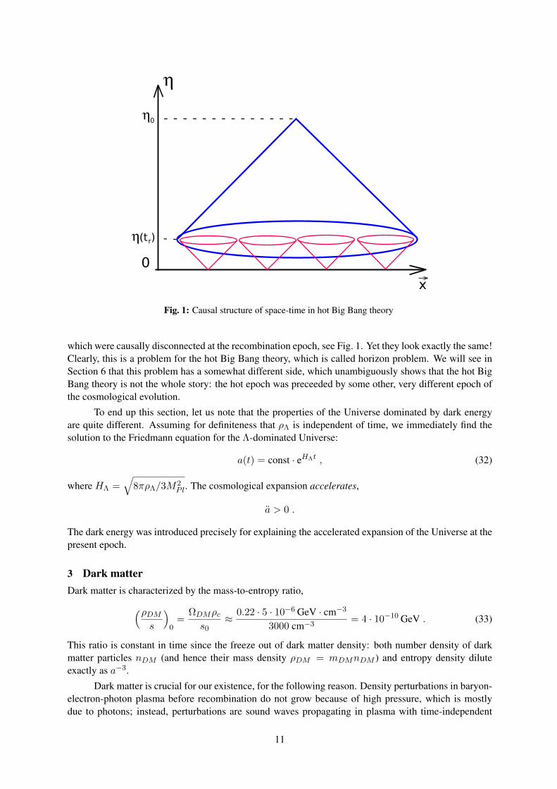
Fig. 1: Causal structure of space-time in hot Big Bang theory

which were causally disconnected at the recombination epoch, see Fig. 1. Yet they look exactly the same!Clearly, this is a problem for the hot Big Bang theory, which is called horizon problem. We will see inSection 6 that this problem has a somewhat different side, which unambiguously shows that the hot BigBang theory is not the whole story: the hot epoch was preceeded by some other, very different epoch ofthe cosmological evolution.

To end up this section, let us note that the properties of the Universe dominated by dark energyare quite different. Assuming for definiteness that ρΛ is independent of time, we immediately find thesolution to the Friedmann equation for the Λ-dominated Universe:

a(t) = const · eHΛt , (32)

where HΛ =√

8πρΛ/3M2Pl. The cosmological expansion accelerates,

a > 0 .

The dark energy was introduced precisely for explaining the accelerated expansion of the Universe at thepresent epoch.

3 Dark matterDark matter is characterized by the mass-to-entropy ratio,

(ρDMs

)0

=ΩDMρcs0

≈ 0.22 · 5 · 10−6 GeV · cm−3

3000 cm−3= 4 · 10−10 GeV . (33)

This ratio is constant in time since the freeze out of dark matter density: both number density of darkmatter particles nDM (and hence their mass density ρDM = mDMnDM ) and entropy density diluteexactly as a−3.

Dark matter is crucial for our existence, for the following reason. Density perturbations in baryon-electron-photon plasma before recombination do not grow because of high pressure, which is mostlydue to photons; instead, perturbations are sound waves propagating in plasma with time-independent

11

amplitudes. Hence, in a Universe without dark matter, density perturbations in baryonic componentwould start to grow only after baryons decouple from photons, i.e., after recombination. The mechanismof the growth is pretty simple: an overdense region gravitationally attracts surrounding matter; this matterfalls into the overdense region, and the density contrast increases. In the expanding matter dominatedUniverse this gravitational instability results in the density contrast growing like (δρ/ρ)(t) ∝ a(t).Hence, in a Universe without dark matter, the growth factor for baryon density perturbations would be atmost4

a(t0)

a(trec)= 1 + zrec =

TrecT0≈ 103 . (34)

The initial amplitude of density perturbations is very well known from the CMB anisotropy measure-ments, (δρ/ρ)i = 5 · 10−5. Hence, a Universe without dark matter would still be pretty homogeneous:the density contrast would be in the range of a few per cent. No structure would have been formed, nogalaxies, no life. No structure would be formed in future either, as the accelerated expansion due to darkenergy will soon terminate the growth of perturbations.

Since dark matter particles decoupled from plasma much earlier than baryons, perturbations indark matter started to grow much earlier. The corresponding growth factor is larger than Eq. (34), so thatthe dark matter density contrast at galactic and sub-galactic scales becomes of order one, perturbationsenter non-linear regime and form dense dark matter clumps at z = 5 − 10. Baryons fall into poten-tial wells formed by dark matter, so dark matter and baryon perturbations develop together soon afterrecombination. Galaxies get formed in the regions where dark matter was overdense originally. Thedevelopment of perturbations in our Universe is shown in Fig. 2. For this picture to hold, dark matterparticles must be non-relativistic early enough, as relativistic particles fly through gravitational wellsinstead of being trapped there. This means, in particular, that neutrinos cannot constitute a considerablepart of dark matter, hence the bound (24).

tΛtrecteq t

Φ

δB

δDM

δγ

Fig. 2: A sketch of the time dependence, in the linear regime, of density contrasts of dark matter, baryons and pho-tons, δDM ≡ δρDM/ρDM , δB and δγ , respectively, as well as the Newtonian potential Φ. teq and tΛ correspondto the transitions from radiation domination to matter domination, and from decelerated expansion to acceleratedexpansion, trec refers to the recombination epoch.

4Because of the presence of dark energy, the growth factor is even somewhat smaller.

12

Depending on the mass of the dark matter particles and mechanism of their production in theearly Universe, dark matter may be cold (CDM) and warm (WDM). Roughly speaking, CDM consistsof heavy particles, while the masses of WDM particles are smaller,

CDM : mDM & 100 keV , (35a)

WDM : mDM = 3 − 30 keV . (35b)

This assumes that the dark matter particles were in thermal (kinteic) equilibrium at some early times, or,more generally, that their kinetic energy was comparable to temperature. This need not be the case forvery weakly interacting particles; a well known example is axions which are cold dark matter candidatesdespite their very small mass. Likewise, very weakly interacting warm dark matter particles may bemuch heavier than Eq. (35b) suggests.

We will discuss warm dark matter option later on, and now we move on to CDM.

3.1 WIMPS: best guess for cold dark matterThere is a simple mechanism of the dark matter generation in the early Universe. It applies to cold darkmatter. Because of its simplicity and robustness, it is considered by many as a very likely one, and thecorresponding dark matter candidates — weakly interacting massive particles, WIMPs — as the bestcandidates. Let us describe this mechanism in some detail.

Let us assume that there exists a heavy stable neutral particle Y , and that Y -particles can only bedestroyed or created via their pair-annihilation or creation, with annihilation products being the particlesof the Standard Model. We will see that the overall cosmological behaviour of Y -particles is as follows.At high temperatures, T mY , the Y -particles are in thermal equilibrium with the rest of cosmicplasma; there are lots of Y -particles in the plasma, which are continuously created and annihilate. Asthe temperature drops below mY , the equilibrium number density decreases. At some “freeze-out”temperature Tf the number density becomes so small, that Y -particles can no longer meet each otherduring the Hubble time, and their annihilation terminates. After that the number density of survived Y ’sdecreases like a−3, and these relic particles contribute to the mass density in the present Universe. Ourpurpose is to estimate the range of properties of Y -particles, in which they serve as dark matter.

Assuming thermal equilibrium, elementary considerations of mean free path of a particle in gasgive for the lifetime of a non-relativistic Y -particle in cosmic plasma, τann,

σann · v · τann · nY ∼ 1 ,

where v is the velocity of Y -particle, σann is the annihilation cross section at velocity v and nY is theequilibrium number density given by the Boltzmann law at zero chemical potential,

nY = gY ·(mY T

2π

)3/2

e−mYT ,

where gY is the number of spin states of Y -particle. Note that we consider non-relativistic regime,mY T . Let us introduce the notation

σannv = σ0

(in fact, the left hand side is to be understood as thermal average). If the annihilation occurs in s-wave,then σ0 is a constant independent of temperature, for p-wave it is somewhat suppressed at T mY .One should compare the lifetime with the Hubble time, or annihilation rate Γann ≡ τ−1

ann with theexpansion rate H . At T ∼ mY , the equilibrium density is of order nY ∼ T 3, and Γann H for nottoo small σ0. This means that annihilation (and, by reciprocity, creation) of Y -pairs is indeed rapid, andY -particles are indeed in thermal equilibrium with the plasma. At very low temperature, on the otherhand, the equilibrium number density n(eq)

Y is exponentially small, and the equilibrium rate is small,

13

Γ(eq)ann H . At low temperatures we cannot, of course, make use of the equilibrium formulas: Y -

particles no longer annihilate (and, by reciprocity, are no longer created), there is no thermal equilibriumwith respect to creation–annihilation processes, and the number density nY gets diluted only because ofthe cosmological expansion.

The freeze-out temperature Tf is determined by the relation

τ−1ann ≡ Γann ∼ H ,

where we can still use the equilibrium formulas, as Y -particles are in thermal equilibrium (with respectto annihilation and creation) just before freeze-out. Making use of the relation (29) between the Hubbleparameter and temperature at radiation domination, we obtain

σ0(Tf ) · nY (Tf ) ∼T 2f

M∗Pl, (36)

or

σ0(Tf ) · gY ·(mY Tf

2π

)3/2

e−mYTf ∼

T 2f

M∗Pl.

The latter equation gives the freeze-out temperature, which, up to loglog corrections, is

Tf ≈mY

ln(M∗PlmY σ0)(37)

(the possible depndence of σ0 on temperature is irrelevant in the right hand side: we are doing thecalculation in the leading-log approximation anyway). Note that this temperature is somewhat lower thanmY , if the relevant microscopic mass scale is much below MPl. This means that Y -particles freeze outwhen they are indeed non-relativistic, hence the term “cold dark matter”. The fact that the annihilationand creation of Y -particles terminate at relatively low temperature has to do with rather slow expansionof the Universe, which should be compensated for by the smallness of the number density nY .

At the freeze-out temperature, we make use of Eq. (36) and obtain

nY (Tf ) =T 2f

M∗Plσ0(Tf ).

Note that this density is inversely proportional to the annihilation cross section (modulo logarithm). Thereason is that for higher annihilation cross section, the creation–annihilation processes are longer inequilibrium, and less Y -particles survive.

Up to a numerical factor of order 1, the number-to-entropy ratio at freeze-out is

nYs' 1

g∗(Tf )M∗PlTfσ0(Tf ). (38)

This ratio stays constant until the present time, so the present number density of Y -particles is nY,0 =s0 · (nY /s)freeze−out, and the mass-to-entropy ratio is

ρY,0s0

=mY nY,0s0

' ln(M∗PlmY σ0)

g∗(Tf )M∗Plσ0(Tf )' ln(M∗PlmY σ0)√

g∗(Tf )MPlσ0(Tf ),

where we made use of Eq. (37). This formula is remarkable. The mass density depends mostly on oneparameter, the annihilation cross section σ0. The dependence on the mass of Y -particle is through thelogarithm and through g∗(Tf ); it is very mild. The value of the logarithm here is between 30 and 40,depending on parameters (this means, in particular, that freeze-out occurs when the temperature drops30 to 40 times below the mass of Y -particle). Plugging in other numerical values (g∗(Tf ) ∼ 100,

14

M∗Pl ∼ 1018 GeV), as well as numerical factor omitted in Eq. (38), and comparing with Eq. (33) weobtain the estimate

σ0(Tf ) ≡ 〈σv〉(Tf ) = (1÷ 2) · 10−36 cm2 . (39)

This is a weak scale cross section, which tells us that the relevant energy scale is TeV. We note in passingthat the estimate (39) is quite precise and robust.

If the annihilation occurs in s-wave, the annihilation cross section may be parametrized as σ0 =α2/M2 where α is some coupling constant, andM is a mass scale (which may be higher thanmY ). Thisparametrization is suggested by the picture of Y pair-annihilation via the exchange by another particleof mass M . With α ∼ 10−2, the estimate for the mass scale is roughly M ∼ 1 TeV. Thus, withvery mild assumptions, we find that the non-baryonic dark matter may naturally originate from the TeV-scale physics. In fact, what we have found can be understood as an approximate equality between thecosmological parameter, mass-to-entropy ratio of dark matter, and the particle physics parameters,

mass-to-entropy ' 1

MPl

(TeVαW

)2

.

Both are of order 10−10 GeV, and it is very tempting to think that this is not a mere coincidence. If it isnot, the dark matter particle should be found at the LHC.

Of course, the most prominent candidate for WIMP is neutralino of the supersymmetric exten-sions of the Standard Model. The situation with neutralino is somewhat tense, however. The point isthat the pair-annihilation of neutralinos often occurs in p-wave, rather than s-wave. This gives the sup-pression factor in σ0 ≡ 〈σannv〉, proportional to v2 ∼ Tf/mY ∼ 1/30. Hence, neutralinos tend to beoverproduced in most of the parameter space of MSSM and other models. Yet neutralino remains a goodcandidate, especially at high tanβ.

3.2 Warm dark matter: light gravitinosThe cold dark matter scenario successfully describes the bulk of the cosmological data. Yet, there areclouds above it. First, according to numerical simulations, CDM scenario tends to overproduce smallobjects — dwarf galaxies: it predicts hundreds of satellite dwarf galaxies in the vicinity of a large galaxylike Milky Way, whereas only dozens of satellites have been observed so far. Second, again accordingto simulations, CDM tends to produce too high densities in galactic centers (cusps in density profiles);this feature is not confirmed by observations either. There is no strong discrepancy yet, but one may bemotivated to analyse a possibility that dark matter is not that cold.

An alternative to CDM is warm dark matter whose particles decouple being relativistic. Let usassume for definiteness that they are in kinetic equilibrium with cosmic plasma when their number den-sity freezes out (thermal relic). After kinetic equilibrium breaks down, and WDM particles decouplecompletely, their spatial momenta decrease as a−1, i.e., the momenta are of order T all the time afterdecoupling. WDM particles become non-relativistic at T ∼ m, where m is their mass. Only afterthat the WDM perturbations start to grow5: as we mentioned above, relativistic particles escape fromgravitational potentials, so the gravitational potentials get smeared out instead of getting deeper. Beforebecoming non-relativistic, WDM particles travel the distance of the order of the horizon size; the WDMperturbations therefore are suppressed at those scales. The horizon size at the time tnr when T ∼ m isof order

l(tnr) ' H−1(T ∼ m) =M∗PlT 2∼ M∗Pl

m2.

Due to the expansion of the Universe, the corresponding length at present is

l0 = l(tnr)a0

a(tnr)∼ l(tnr)

T

T0∼ MPl

mT0, (40)

5The situation in fact is somewhat more complicated, but this simplified picture will be sufficient for our estimates.

15

where we neglected (rather weak) dependence on g∗. Hence, in WDM scenario, structures of sizessmaller than l0 are less abundant as compared to CDM. Let us point out that l0 refers to the size of theperturbation as if it were in the linear regime; in other words, this is the size of the region from whichmatter collapses into a compact object.

The present size of a dwarf galaxy is a few kpc, and the density is about 106 of the average densityin the Universe. Hence, the size l0 for these objects is of order 100 kpc ' 3 · 1023 cm. Requiring thatperturbations of this size, but not much larger, are suppressed, we obtain from Eq. (40) the estimate (35b)for the mass of WDM particles.

Among WDM candidates, light gravitino is probably the best motivated. The gravitino mass is oforder

m3/2 'F

MPl,

where√F is the supersymmetry breaking scale. Hence, gravitino masses are in the right ballpark for

rather low supersymmetry breaking scales,√F ∼ 106 − 107 GeV. This is the case, e.g., in gauge

mediation scenario. With so low mass, gravitino is the lightest supersymmetric particle (LSP), so it isstable in many supersymmetric extensions of the Standard Model. From this viewpoint gravitinos canindeed serve as dark matter particles. For what follows, important parameters are the widths of decaysof other superpartners into gravitino and the Standard Model particles. These are of order

ΓS 'M5S

F 2'

M5S

m23/2M

2Pl

, (41)

where MS is the mass of the superpartner.

One mechanism of the gravitino production in the early Universe is decays of other superpartners.Gravitino interacts with everything else so weakly, that once produced, it moves freely, without inter-acting with cosmic plasma. At production, gravitinos are relativistic, hence they are indeed warm darkmatter candidates. Let us assume that production in decays is the dominant mechanism and considerunder what circumstances the present mass density of gravitinos coincides with that of dark matter.

The rate of gravitino production in decays of superpartners of the type S in the early Universe is

d(n3/2/s)

dt=nSs

ΓS ,

where n3/2 and nS are number densities of gravitinos and superpartners, respectively, and s is the entropydensity. For superpartners in thermal equilibrium, one has nS/s = const ∼ g−1

∗ for T & MS , andnS/s ∝ exp(−MS/T ) at T MS . Hence, the production is most efficient at T ∼ MS , when thenumber density of superpartners is still large, while the Universe expands most slowly. The density ofgravitinos produced in decays of S’s is thus given by

n3/2

s'(d(n3/2/s)

dt·H−1

)

T∼MS

' ΓSg∗H−1(T ∼MS) ' 1

g∗·

M5S

m23/2M

2Pl

· M∗Pl

M2S

.

This gives the mass-to-entropy ratio today:

m3/2n3/2

s'∑

S

M3S

g3/2∗ MPlm3/2

, (42)

where the sum runs over all superpartner species which have ever been relativistic in thermal equilibrium.The correct value (33) is obtained for gravitino masses in the range (35b) at

MS = 100− 300 GeV . (43)

16

Thus, the scenario with gravitino as warm dark matter particle requires light superpartners, which are tobe discovered at the LHC.

A few comments are in order. First, decays of superpartners is not the only mechanism of gravitinoproduction: gravitinos may also be produced in scattering of superpartners. To avoid overproduction ofgravitinos in the latter processes, one has to assume that the maximum temperature in the Universe(reached after post-inflationary reheating stage) is quite low, Tmax ∼ 1 − 10 TeV. This is not a par-ticularly plausible assumption, but it is consistent with everything else in cosmology and can indeedbe realized in some models of inflation. Second, existing constraints on masses of strongly interactingsuperpartners (gluinos and squarks) suggest that their masses exceed Eq. (43). Hence, these particlesshould not contribute to the sum in Eq. (42), otherwise WDM gravitinos would be overproduced. Thisis possible, if masses of squarks and gluinos are larger than Tmax, so that they were never abundant inthe early Universe. Third, gravitino produced in decays of superpartners is not a thermal relic, as it wasnever in thermal equilibrium with the rest of cosmic plasma. Nevertheless, since gravitinos are producedat T ∼ MS and at that time have energy E ∼ MS ∼ T , our estimate (40) does apply. Finally, thedecay into gravitino and the Standard Model particles is the only decay channel for the next-to-lightestsuperpartner (NLSP). Hence, the estimate for the total width of NLSP is given by Eq. (41), so that

cτNLSP = a few ·mm− a few · 100 m

form2/3 = 3−30 keV andMNLSP = 100−300 GeV. Thus, NLSP should either be visible in a detector,or fly it through.

Needless to say, the warm gravitino scenario is a lot more contrived than the WIMP option. It isreassuring, however, that it can be ruled out or confirmed at the LHC.

3.3 DiscussionIf dark matter particles are indeed WIMPs, and the relevant energy scale is of order 1 TeV, then the HotBig Bang theory will be probed experimentally up to temperature of (a few) · (10− 100) GeV and downto age 10−9 − 10−11 s in relatively near future (compare to 1 MeV and 1 s accessible today through BigBang Nucleosynthesis). With microscopic physics to be known from collider experiments, the WIMPdensity will be reliably calculated and checked against the data from observational cosmology. Thus,WIMP scenario offers a window to a very early stage of the evolution of the Universe.

If dark matter particles are gravitinos, the prospect of probing quantitatively so early stage of thecosmological evolution is not so bright: it would be very hard, if at all possible, to get an experimentalhandle on the gravitino mass; furthermore, the present gravitino mass density depends on an unknownreheat temperature Tmax. On the other hand, if this scenario is realized in Nature, then the whole pictureof the early Universe will be quite different from our best guess on the early cosmology. Indeed, gravitinoscenario requires low reheat temperature, which in turn calls for rather exotic mechanism of inflation.

The mechanisms discussed here are by no means the only ones capable of producing dark matter,and WIMPs and gravitinos are by no means the only candidates for dark matter particles. Other darkmatter candidates include axions, sterile neutrinos, Q-balls, very heavy relics produced towards the endof inflation, etc. Hence, even though there are grounds to hope that the dark matter problem will besolved by the LHC, there is no guarantee at all.

4 Baryon asymmetry of the UniverseIn the present Universe, there are baryons and almost no antibaryons. The number density of baryonstoday is characterized by the ratio ηB , see Eq. (18). In the early Universe, the appropriate quantity is

∆B =nB − nB

s,

17

where nB is the number density of antibaryons, and s is the entropy density. If the baryon numberis conserved, and the Universe expands adiabatically, ∆B is constant, and its value, up to a numericalfactor, is equal to η (cf. Eqs. (11) and (15)). More precisely,

∆B ≈ 0.8 · 10−10 .

At early times, at temperatures well above 100 MeV, cosmic plasma contained many quark-antiquarkpairs, whose number density was of the order of the entropy density,

nq + nq ∼ s ,

while the baryon number density was related to densities of quarks and antiquarks as follows (baryonnumber of a quark equals 1/3),

nB =1

3(nq − nq) .

Hence, in terms of quantities characterizing the very early epoch, the baryon asymmetry may be ex-pressed as

∆B ∼nq − nqnq + nq

.

We see that there was one extra quark per about 10 billion quark-antiquark pairs! It is this tiny excessthat is responsible for the entire baryonic matter in the present Universe: as the Universe expanded andcooled down, antiquarks annihilated with quarks, and only the excessive quarks remained and formedbaryons.

There is no logical contradiction to suppose that the tiny excess of quarks over antiquarks was builtin as an initial condition. This is not at all satisfactory for a physicist, however. Furthermore, inflationaryscenario does not provide such an initial condition for the hot Big Bang epoch; rather, inflation theorypredicts that the Universe was baryon-symmetric just after inflation. Hence, one would like to explainthe baryon asymmetry dynamically.

The baryon asymmetry may be generated from initially symmetric state only if three necessaryconditions, dubbed Sakharov’s conditions, are satisfied. These are

(i) baryon number non-conservation;

(ii) C- and CP-violation;

(iii) deviation from thermal equilibrium.

All three conditions are easily understood. (i) If baryon number were conserved, and initial netbaryon number in the Universe was zero, the Universe today would still be symmetric. (ii) If C or CPwere conserved, then the rate of reactions with particles would be the same as the rate of reactions withantiparticles, and no asymmetry would be generated. (iii) Thermal equilibrium means that the systemis stationary (no time dependence at all). Hence, if the initial baryon number is zero, it is zero forever,unless there are deviations from thermal equilibrium.

There are two well understood mechanisms of baryon number non-conservation. One of thememerges in Grand Unified Theories and is due to the exchange of super-massive particles. It is similar,say, to the mechanism of charm non-conservation in weak interactions, which occurs via the exchange ofheavy W -bosons. The scale of these new, baryon number violating interactions is the Grand Unificationscale, presumably of order MGUT ' 1016 GeV. It is rather unlikely that the baryon asymmetry wasgenerated due to this mechanism: the relevant temperature would be of order MGUT , while so highreheat temperature after inflation is difficult to obtain.

Another mechanism is non-perturbative [12] and is related to the triangle anomaly in the baryoniccurrent (a keyword here is “sphaleron” [13, 14]). It exists already in the Standard Model, and, possiblywith slight modifications, operates in all its extensions. The two main features of this mechanism, as

18

applied to the early Universe, is that it is effective over a wide range of temperatures, 100 GeV < T <1011 GeV, and that it conserves (B − L).

Let us pause here to discuss the physics behind electroweak baryon and lepton number non-conservation in little more detail, though still at a qualitative level. A detailed analysis can be foundin the book [15] and in references therein.

The first object to consider is the baryonic current,

Bµ =1

3·∑

i

qiγµqi ,

where the sum runs over quark flavors. Naively, the baryonic current is conserved, but at the quantumlevel its divergence is non-zero, the effect called triangle anomaly (similar effect goes under the name ofaxial anomaly in the context of QED and QCD),

∂µBµ =

1

3· 3colors · 3generations ·

g2

32π2εµνλρF aµνF

aλρ ,

where F aµν and g are the field strength of the SU(2)W gauge field and the SU(2)W gauge coupling,respectively. Likewise, each leptonic current (n = e, µ, τ ) is anomalous,

∂µLµn =

g2

32π2· εµνλρF aµνF aλρ .

A non-trivial fact is that there exist large field fluctuations, F aµν(x, t) ∝ g−1 which have

Q ≡∫

d3xdtg2

32π2· εµνλρF aµνF aλρ 6= 0 .

Furthermore, for any such fluctuation the value of Q is integer. Suppose now that a fluctuation withnon-vanishing Q has occured. Then the baryon numbers in the end and beginning of the process aredifferent,

Bfin −Bin =

∫d3xdt ∂µB

µ = 3Q . (44)

LikewiseLn, fin − Ln, in = Q . (45)

This explains the selection rule mentioned above: B is violated, (B − L) is not.

At zero temprature, the large field fluctuations that induce baryon and lepton number violationare vacuum fluctuations, called instantons, which to a certain extent are similar to virtual fields thatemerge and disappear in vacuum of quantum field theory at the perturbative level. The peculiarity is thatinstantons are large field fluctuations. The latter property results in the exponential suppression of theprobability of their emergence, and hence the rate of baryon number violating processes, by a factor

e−16π2

g2 ∼ 10−165 .

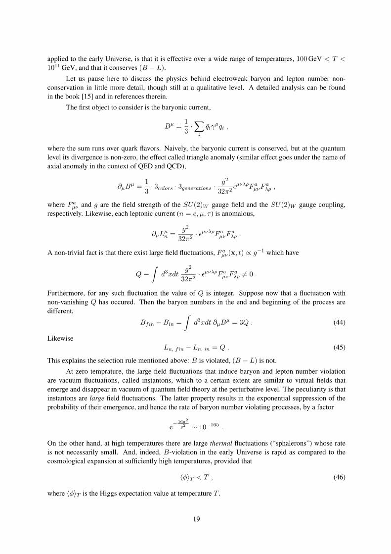
On the other hand, at high temperatures there are large thermal fluctuations (“sphalerons”) whose rateis not necessarily small. And, indeed, B-violation in the early Universe is rapid as compared to thecosmological expansion at sufficiently high temperatures, provided that

〈φ〉T < T , (46)

where 〈φ〉T is the Higgs expectation value at temperature T .

19

One may wonder how baryon number may be not conserved even though there are no baryonnumber violating terms in the Lagrangian of the Standard Model. To understand what is going on, letus consider a massless left handed fermion field in the background of the SU(2) gauge field A(x, t),which depends on space-time coordinates in a non-trivial way. As a technicality, we set the temporalcomponent of the gauge field equal to zero, A0 = 0, by the choice of gauge. One way to understand thebehavior of the fermion field in the gauge field background is to study the system of eigenvalues of theDirac Hamiltonian ω(t). The Hamiltonian is defined in the standard way

HDirac(t) = iαi (∂i − igAi(x, t))1− γ5

2,

where αi = γ0γi, so that the Dirac equation has the Schrödinger form,

i∂ψ

∂t= HDiracψ .

We are going to discuss the eigenvalues ωn(t) of the operator HDirac(t), treating t as a parameter. Theseeigenvalues are found from

HDirac(t)ψn = ωn(t)ψn .

At A = 0 the system of levels is shown schematically in Fig. 3. Importantly, there are both positive-and negative-energy levels. According to Dirac, the lowest energy state (Dirac vacuum) has all negativeenergy levels occupied, and all positive energy levels empty. Occupied positive energy levels (three ofthem in Fig. 3) correspond to real fermions, while empty negative energy levels describe antifermions(one in Fig. 3). Fermion-antifermion annihilation in this picture is a jump of a fermion from a positiveenergy level to an unoccupied negative energy level.

As a side remark, this original Dirac picture is, in fact, equivalent to the more conventional (bynow) procedure of the quantization of fermion field, which does not make use of the notion of negativeenergy levels. The discussion that follows can be translated into the conventional language; however, theoriginal Dirac picture turnd out to be a lot more transparent in our context. This is a nice example of thecomplementarity of various approaches in quantum field theory.

Let us proceed with the discussion of the fermion energy levels in gauge field backgrounds. Inweak background fields, the energy levels depend on time (move), but nothing dramatic happens. Foradiabatically varying background fields, the fermions merely sit on their levels, while fast changingfields generically give rise to jumps from, say, negative- to positive-energy levels, that is, creation offermion-antifermion pairs. Needless to say, fermion number (Nf −Nf ) is conserved.

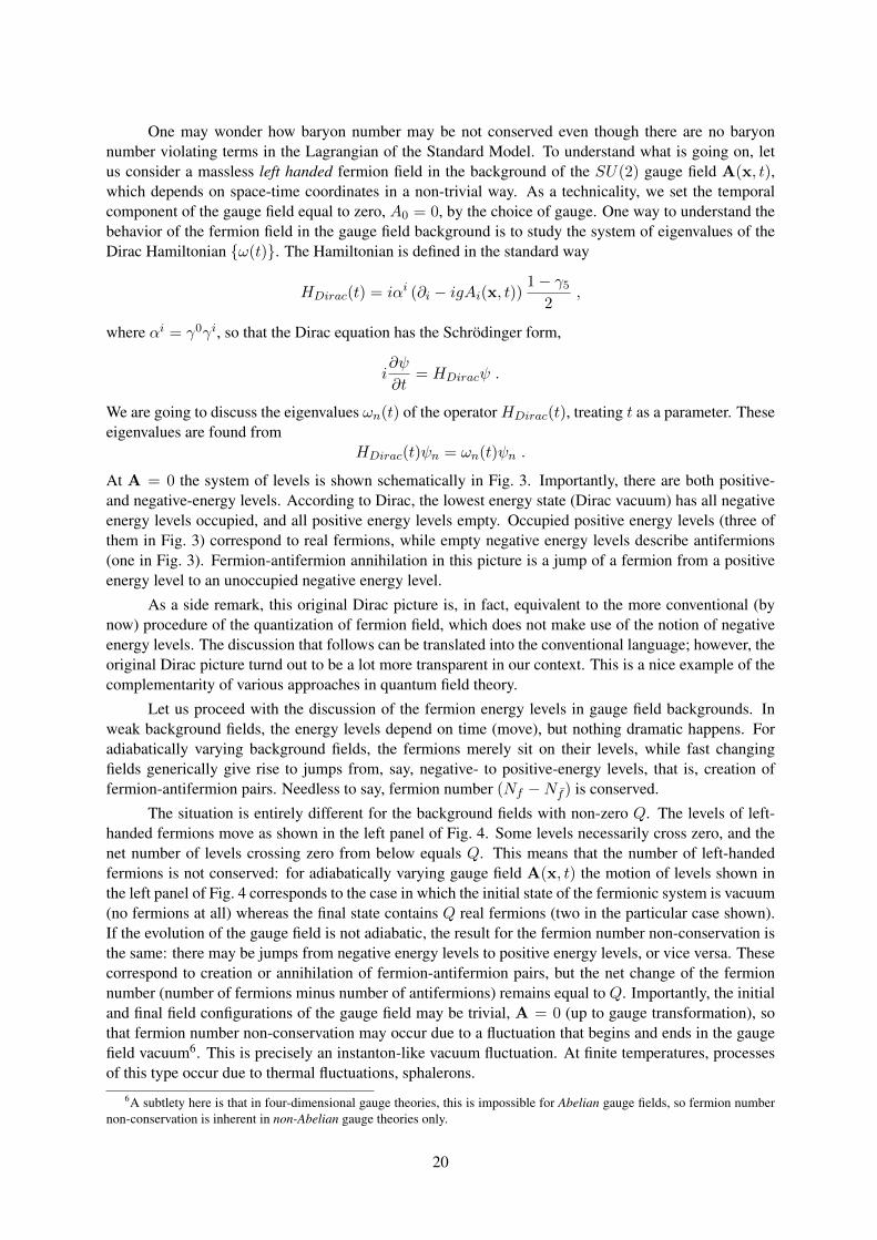
The situation is entirely different for the background fields with non-zero Q. The levels of left-handed fermions move as shown in the left panel of Fig. 4. Some levels necessarily cross zero, and thenet number of levels crossing zero from below equals Q. This means that the number of left-handedfermions is not conserved: for adiabatically varying gauge field A(x, t) the motion of levels shown inthe left panel of Fig. 4 corresponds to the case in which the initial state of the fermionic system is vacuum(no fermions at all) whereas the final state contains Q real fermions (two in the particular case shown).If the evolution of the gauge field is not adiabatic, the result for the fermion number non-conservation isthe same: there may be jumps from negative energy levels to positive energy levels, or vice versa. Thesecorrespond to creation or annihilation of fermion-antifermion pairs, but the net change of the fermionnumber (number of fermions minus number of antifermions) remains equal to Q. Importantly, the initialand final field configurations of the gauge field may be trivial, A = 0 (up to gauge transformation), sothat fermion number non-conservation may occur due to a fluctuation that begins and ends in the gaugefield vacuum6. This is precisely an instanton-like vacuum fluctuation. At finite temperatures, processesof this type occur due to thermal fluctuations, sphalerons.

6A subtlety here is that in four-dimensional gauge theories, this is impossible for Abelian gauge fields, so fermion numbernon-conservation is inherent in non-Abelian gauge theories only.

20

ω

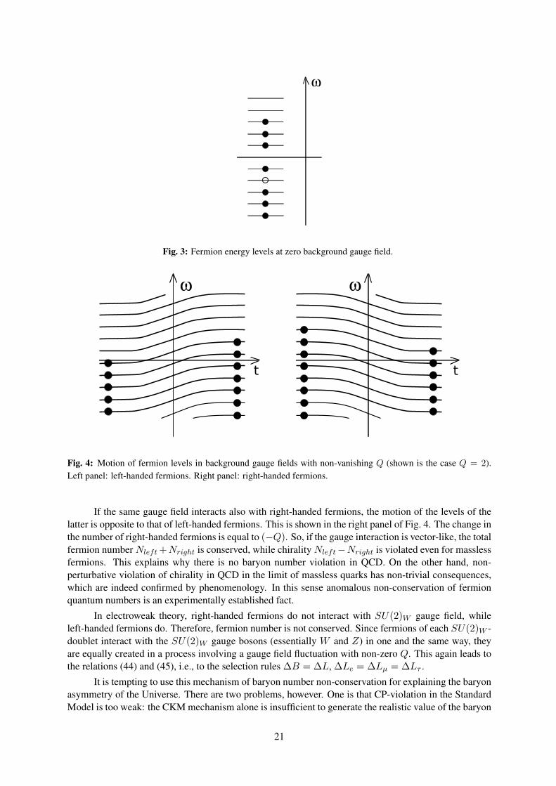
Fig. 3: Fermion energy levels at zero background gauge field.

ω

t

ω

t

Fig. 4: Motion of fermion levels in background gauge fields with non-vanishing Q (shown is the case Q = 2).Left panel: left-handed fermions. Right panel: right-handed fermions.

If the same gauge field interacts also with right-handed fermions, the motion of the levels of thelatter is opposite to that of left-handed fermions. This is shown in the right panel of Fig. 4. The change inthe number of right-handed fermions is equal to (−Q). So, if the gauge interaction is vector-like, the totalfermion number Nleft+Nright is conserved, while chirality Nleft−Nright is violated even for masslessfermions. This explains why there is no baryon number violation in QCD. On the other hand, non-perturbative violation of chirality in QCD in the limit of massless quarks has non-trivial consequences,which are indeed confirmed by phenomenology. In this sense anomalous non-conservation of fermionquantum numbers is an experimentally established fact.

In electroweak theory, right-handed fermions do not interact with SU(2)W gauge field, whileleft-handed fermions do. Therefore, fermion number is not conserved. Since fermions of each SU(2)W -doublet interact with the SU(2)W gauge bosons (essentially W and Z) in one and the same way, theyare equally created in a process involving a gauge field fluctuation with non-zero Q. This again leads tothe relations (44) and (45), i.e., to the selection rules ∆B = ∆L, ∆Le = ∆Lµ = ∆Lτ .

It is tempting to use this mechanism of baryon number non-conservation for explaining the baryonasymmetry of the Universe. There are two problems, however. One is that CP-violation in the StandardModel is too weak: the CKM mechanism alone is insufficient to generate the realistic value of the baryon

21

asymmetry. Hence, one needs extra sources of CP-violation. Another problem has to do with departurefrom thermal equilibrium that is necessary for the generation of the baryon asymmetry. At temperatureswell above 100 GeV electroweak symmetry is restored, the expectation value of the Higgs field φ iszero7, the relation (46) is valid, and the baryon number non-conservation is rapid as compared to thecosmological expansion. At temperatures of order 100 GeV the relation (46) may be violated, but theUniverse expands very slowly: the cosmological time scale at these temperatures is

H−1 =M∗PlT 2∼ 10−10 s , (47)

which is very large by the electroweak physics standards. The only way in which strong departure fromthermal equilibrium at these temperatures may occur is through the first order phase transition.

Veff (φ) Veff (φ)

φ φ

Fig. 5: Effective potential as function of φ at different temperatures. Left: first order phase transition. Right:second order phase transition. Upper curves correspond to higher temperatures.

The property that at temperatures well above 100 GeV the expectation value of the Higgs field iszero, while it is non-zero in vacuo, suggests that there may be a phase transition from the phase with〈φ〉 = 0 to the phase with 〈φ〉 6= 0. The situation is pretty subtle here, as φ is not gauge invariant, andhence cannot serve as an order parameter, so the notion of phases with 〈φ〉 = 0 and 〈φ〉 6= 0 is vague.In fact, neither electroweak theory nor most of its extensions have a gauge-invariant order parameter, sothere is no real distinction between these “phases”. This situation is similar to that in liquid-vapor system,which does not have an order parameter and may or may not experience vapor-liquid phase transition astemperature decreases, depending on other parameters characterizing this system, e.g., pressure. In theStandard Model the role of such a parameter is played by the Higgs self-coupling λ or, in other words,the Higgs boson mass.

Continuing to use somewhat sloppy terminology, we observe that the interesting case for us isthe first order phase transition. In this case the effective potential (free energy density as function of

7There are subtleties at this point, see below.

22

φ) behaves as shown in the left panel of Fig. 5. At high temperatures, there exists one minimum ofVeff at φ = 0, and the expectation value of the Higgs field is zero. As the temperature decreases,another minimum appears at finite φ, and then becomes lower than the minimum at φ = 0. However,the probability of the transition from the phase φ = 0 to the phase φ 6= 0 is very small for some time,so the system gets overcooled. The transition occurs when the temperature becomes sufficiently low, asshown schematically by an arrow in Fig. 5. This is to be contrasted to the case, e.g., of the second orderphase transition with the behavior of the effective potential shown in the right panel of Fig. 5. In thelatter case, the field slowly evolves, as the temperature decreases, from zero to non-zero vacuum value,and the system remains very close to the thermal equilibrium at all times.

φ = 0

φ 6= 0φ 6= 0

φ = 0

φ 6= 0

φ = 0

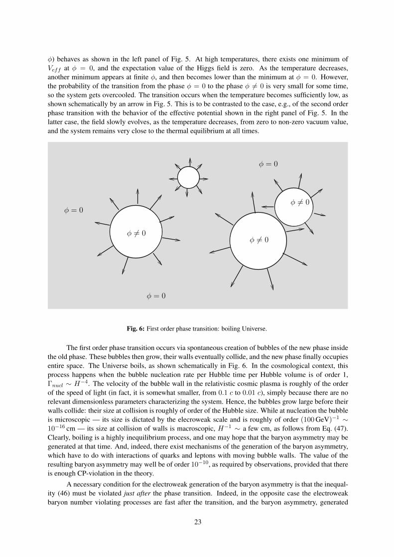
Fig. 6: First order phase transition: boiling Universe.

The first order phase transition occurs via spontaneous creation of bubbles of the new phase insidethe old phase. These bubbles then grow, their walls eventually collide, and the new phase finally occupiesentire space. The Universe boils, as shown schematically in Fig. 6. In the cosmological context, thisprocess happens when the bubble nucleation rate per Hubble time per Hubble volume is of order 1,Γnucl ∼ H−4. The velocity of the bubble wall in the relativistic cosmic plasma is roughly of the orderof the speed of light (in fact, it is somewhat smaller, from 0.1 c to 0.01 c), simply because there are norelevant dimensionless parameters characterizing the system. Hence, the bubbles grow large before theirwalls collide: their size at collision is roughly of order of the Hubble size. While at nucleation the bubbleis microscopic — its size is dictated by the elecroweak scale and is roughly of order (100 GeV)−1 ∼10−16 cm — its size at collision of walls is macroscopic, H−1 ∼ a few cm, as follows from Eq. (47).Clearly, boiling is a highly inequilibrium process, and one may hope that the baryon asymmetry may begenerated at that time. And, indeed, there exist mechanisms of the generation of the baryon asymmetry,which have to do with interactions of quarks and leptons with moving bubble walls. The value of theresulting baryon asymmetry may well be of order 10−10, as required by observations, provided that thereis enough CP-violation in the theory.

A necessary condition for the electroweak generation of the baryon asymmetry is that the inequal-ity (46) must be violated just after the phase transition. Indeed, in the opposite case the electroweakbaryon number violating processes are fast after the transition, and the baryon asymmetry, generated

23

during the transition, is washed out afterwards. Hence, the phase transition must be of strong enoughfirst order. This is not the case in the Standard Model. To see why this is so, and to get an idea in whichextensions of the Standard Model the phase transition may be of strong enough first order, let us considerthe effective potential in some detail. At zero temperature, the Higgs potential has the standard fom,

V (φ) = −m2

2|φ|2 +

λ

4|φ|4 .

Here

|φ| ≡(φ†φ)1/2

(48)

is the length of the Higgs doublet φ, m2 = λv2 and v = 247 GeV is the Higgs expectation value invacuo. The Higgs boson mass is related to the latter as follows,

mH =√

2λv . (49)

Now, to the leading order of perturbation theory, the finite temperature effects modify the effective po-tential into

Veff (φ, T ) =α

2|φ|2 − β

3T |φ|3 +

λ

4|φ|4 , (50)

with α(T ) = −m2 + g2T 2, where g2 is a positive linear combination of squares of coupling constantsof all fields to the Higgs field (in the Standard Model, a linear combination of g2, g′ 2 and y2

i , where gand g′ are gauge couplings and yi are Yukawa couplings), while β is a positive linear combination ofcubes of coupling constants of all bosonic fields to the Higgs field. In the Standard Model, β is a linearcombination of g3 and g′ 3, i.e., a linear combination of M3

W /v3 and M3

Z/v3,

β =1

2π

2M3W +M3

Z

v3. (51)

The cubic term in Eq. (50) is rather peculiar: in view of Eq. (48) it is not analytic in the original Higgsfield φ. Yet this term is crucial for the first order phase transition: for β = 0 the phase transition wouldbe of the second order. The origin of the non-analytic cubic term can be traced back to the enhancementof the Bose–Einstein thermal distribution at low momenta, p,m T ,

fBose(p) =1

e

√p2+m2

aT − 1

' T√p2 +m2

a

,

where ma ' ga|φ| is the mass of the boson a that is generated due to the non-vanishing Higgs field, andga is the coupling constant of the field a to the Higgs field. Clearly, at p ga|φ| the distribution functionis non-analytic in φ,

fBose(p) 'T

ga|φ|.

It is this non-analyticity that gives rise to the non-analytic cubic term in the effective potential. Impor-tantly, the Fermi–Dirac distribution,

fFermi(p) =1

e

√p2+m2

aT + 1

,

is analytic in m2a, and hence φ†φ, so fermions do not contribute to the cubic term.

With the cubic term in the effective potential, the phase transition is indeed of the first order:at high temperatures the coefficient α is positive and large, and there is one minimum of the effective

24

potential at φ = 0, while for α small but still positive there are two minima. The phase transition ocursat α ≈ 0; at that moment

Veff (φ, T ) ≈ −βT3|φ|3 +

λ

4|φ|4 .

We find from this expression that immediately after the phase transition the minimum of Veff is at

φ ' βT

λ.

Hence, the necessary condition for successfull electroweak baryogenesis, φ > T , translates into

β > λ . (52)

According to Eq. (49), λ is proportional to m2H , whereas in the Standard Model β is proportional to

(2M3W + M3

Z). Therefore, the relation (52) holds for small Higgs boson masses only; in the StandardModel one makes use of Eqs. (49) and (51) and finds that this happens for mH < 50 GeV, which is ruledout8.

This discussion indicates a possible way to make the electroweak phase transition strong. Whatone needs is the existence of new bosonic fields that have large enough couplings to the Higgs field(s),and hence provide large contriutions to β. To have an effect on the dynamics of the transition, the newbosons must be present in the cosmic plasma at the transition temperature, T ∼ 100 GeV, so their massesshould not be too high, M . 300 GeV. In supersymmetric extensions of the Standard Model, the naturalcandidate for long time has been stop (superpartner of top-quark) whose Yukawa coupling to the Higgsfield is the same as that of top, that is, large. The light stop scenario for electroweak baryogenesis wouldindeed work, as has been shown by the detailed analysis in Ref. [16].

Yet another issue is CP-violation, which has to be strong enough for successfull electroweak baryo-genesis. As the asymmetry is generated in the interactions of quarks and leptons (and their superpartnersin supersymmetric extensions) with the bubble walls, CP-violation must occur at the walls. Recall nowthat the walls are made of the Higgs field(s). This points towards the necessity of CP-violation in theHiggs sector, which may only be the case in a theory with more than one Higgs fields.

To summarize, electroweak baryogenesis requires a considerable extension of the Standard Model,with masses of new particles in the range 100− 300 GeV. Hence, this mechanism will definitely be ruledout or confirmed by the LHC. We stress, however, that electroweak baryogenesis is not the only option atall: an elegant and well motivated competitor is leptogenesis [17]; several other mechanisms have beenproposed that may be responsible for the baryon asymmetry of the Universe.

5 Dark energyDark energy, the famous “substance”, does not clump, unlike dark matter. It gives rise to the acceleratedexpansion of the Universe. As we see from Eq. (32), the Universe with constant energy density shouldexpand exponentially; if the energy density is almost constant, the expansion is almost exponential. Letus make use of the first law of thermodynamics, which for the adiabatic expansion reads

dE = −pdV ,

and apply it to comoving volume, E = ρV , V = a3. We obtain for dark energy

dρΛ = −3da

a(ρΛ + pΛ) ,

8In fact, in the Standard Model with mH > 114GeV, there is no phase transition at all; the electroweak transition is smoothcrossover instead. The latter fact is not visible from the expression (50), but that expression is the lowest order perturbativeresult, while the perturbation theory is not applicable for describing the transition in the Standard Model with large mH .

25

ordρΛ

ρΛ= −3

da

a(1 + w) ,

where we introduced the equation of state parameter w such that

pΛ = wρΛ .

Thus, (almost) time-independent dark energy density corresponds to w ≈ −1, i.e., effective pressure ofdark energy is negative. We emphasize that pressure is by definition a spatial component of the energy-momentum tensor, which in the homogeneous and isotropic situation has the general form

Tµν = diag (ρ, p, p, p) .

Dark energy density does not depend on time at all, if pΛ = −ρΛ, i.e.,

Tµν = ρΛηµν ,

where ηµν is the Minkowski tensor. This is characteristic of vacuum, whose energy-momentum tensormust be Lorentz-covariant. Observationally, w is close to−1 to reasonably good precision. The most ac-curate detrmination, which, however, does not include systematic errors in supernovae data and possibletime-dependence of w, is [9]

w = −0.98± 0.05 . (53)

So, the dark energy density is almost time-independent, indeed.

The problem with dark energy is that its present value is extremely small by particle physicsstandards,

ρDE ≈ 4 GeV/m3 = (2× 10−3 eV)4 .

In fact, there are two hard problems. One is that particle physics scales are much larger than the scalerelevant to the dark energy density, so the dark energy density is zero to an excellent approximation.Another is that it is non-zero nevertheless, and one has to understand its energy scale. To quantify thefirst problem, we recall the known scales of particle physics and gravity,

Strong interactions : ΛQCD ∼ 1 GeV ,Electroweak : MW ∼ 100 GeV ,

Gravitational : Mpl ∼ 1019 GeV .

In principle, vacuum should contribute to ρΛ, and there is absolutely no reason for vacuum to be as lightas it is. The discrepancy here is huge, as one sees from the above numbers.

To elaborate on this point, let us note that the action of gravity plus, say, the Standard Model hasthe general form

S = SEH + SSM − ρΛ,0

∫ √−g d4x ,

where SEH = −(16πGN )−1∫R√−g d4x is the Einstein–Hilbert action of General Relativity, SSM

is the action of the Standard Model and ρΛ,0 is the bare cosmological constant. In order that the vacuumenergy density be almost zero, one needs fantastic cancellations between the contributions of the SandardModel fields into the vacuum energy density, on the one hand, and ρΛ,0 on the other. For example, weknow that QCD has a complicated vacuum structure, and one would expect that the energy density ofQCD combined with ρΛ,0 should be of order (1 GeV)4. Nevertheless, it is not, so at least for QCD,one needs a cancellation on the order of 10−44. If one goes further and considers other interactions, thenumbers get even worse.

26

What are the hints from this “first” cosmological constant problem? There are several options,though not many. One is that the Universe could have a very long prehistory. Extremely long. Thisoption has to do with relaxation mechanisms. Suppose that the original vacuum energy density is indeedlarge, say, comparable to the particle physics scales. Then there must be a mechanism which can relaxthis value down to an acceptably small number. It is easy to convince oneself that this relaxation couldnot happen in the history of the Universe we know of. Instead, the Universe should have a very longprehistory during which this relaxation process might occur. At that prehistoric time, the vacuum in theUniverse must have been exactly the same as our vacuum, so the Universe in its prehistory must havebeen exactly like ours, or almost exactly like ours. Only in that case could a relaxation mechanism work.There are concrete scenarios of this sort [18]. However, at the moment it seems that these scenarios arehardly testable, since this is prehistory.

Another possible hint is towards anthropic selection. The argument that goes back to Weinberg andLinde [19, 20] is that if the cosmological constant were larger, say, by a factor of 100, we simply wouldnot exist: the stars would not have formed because of the fast expansion of the Universe. So, the vacuumenergy density may be selected anthropically. The picture is that the Universe may be much, muchlarger than what we can see, and different large regions of the Universe may have different properties. Inparticular, vacuum energy density may be different in different regions. Now, we are somewhere in theplace where one can live. All the rest is empty of human beings, because there the parameters such asvacum energy density are not suitable for their existence. This is disappointing for a theorist, as this pointof view allows for arbitrary tuning of fundamental parameters. It is hard to disprove this option, on theother hand. We do exist, and this is an experimental fact. The anthropic viewpoint may, though hopefullywill not, get more support from the LHC, if no or insufficient new physics is found there. Indeed, anothercandidate for an environmental quantity is the electroweak scale.

Let us recall in this regard the gauge hierarchy problem: the electroweak scale MW ∼ 100 GeV ismuch lower than the natural scale in gravitational physics, the Planck mass, MPl ∼ 1019 GeV. The elec-troweak scale in the Standard Model is unprotected from large contributions due to high energy physics,and in this sense it is very similar to the cosmological constant. There are various anthropic argumentsshowing that the electroweak scale must be small. A simple example is that if one makes it larger withouttouching other parameters, then quarks would be too heavy. Neutron would be the lightest baryon, andproton would be unstable. There would be no stable hydrogen, and that is presumably inconsistent withour existence. Hence, one of the “solutions” to the gauge hierarchy problem is anthropic.

An interesting part of the story is that unlike the cosmological constant, there are natural waysto make the electroweak scale small and render it small in extensions of the Standard Model, like lowenergy supersymmetry. All these extensions require new physics at TeV energies. So we are in a situationwhere the experiment has to say its word. If it says that none of these extensions is there in Nature, thenwe will have to take the anthropic viewpoint much more seriously than before.

Turning to the “second” cosmological constant problem, we note that the scale 10−3 eV may beassociated with some new light field(s), rather than with vacuum. This implies, in general, that ρΛ

depends on time, i.e., w 6= −1 and w may well depend on time itself. “Normal” field (called quitessencein this context) has w > −1, but there are examples (rather contrived) of fields with w < −1 (calledphantom fields). Current data are compatible with time-independent w equal to −1, but their precisionis not particularly high. We conclude that future cosmological observations may shed new light on thefield content of fundamental theory.

6 Cosmological perturbations and the very early UniverseWith Big Bang nucleosynthesis theory and observations, we are confident of the theory of the earlyUniverse at temperatures up to T ' 1 MeV, that corresponds to age of t ' 1 second. With the LHC, wehope to be able to go up to temperatures T ∼ 100 GeV and age t ∼ 10−10 second. The question is: are

27

we going to have a handle on even earlier epoch?

The key issue in this regard is cosmological perturbations. These are inhomogeneities in the energydensity and assoiated gravitational potentials, in the first place. This type of inhomogeneities is calledscalar perturbations, as they are described by 3-scalars. There may exist perturbations of another type,called tensor; these are primordial gravity waves. We will mostly concentrate on scalar perturbations,since they are observed; tensor perturbations are important too, and we comment on them later on. Itis worth pointing out that perturbations of the present size below ten Megaparsec have large amplitudestoday and are non-linear, but in the past their amplitudes were small, and they can be described within thelinearized theory. Indeed, CMB temperature anisotropy tells us that the perturbations at recombinationepoch were roughly at the level

δ ≡ δρ

ρ= 10−4 − 10−5 .

Thus, the linearized theory works very well before recombination and somewhat later.

Properties of scalar perturbations are mesured in various ways. Perturbations of large spatial scalesleave their imprint in CMB temperature anisotropy and polarization, so we have very detailed knowledgeof them. Shorter wavelength perturbations are studied by analysing distributions of galaxies and quasarsat present and in relatively near past. There are several other methods, some of which can probe evenshorter wavelengths. As we discuss in more detail below, scalar perturbations in the linear regime areactually Gaussian random field, and the first thing to measure is its power spectrum. Overall, independentmethods give consistent results, see Fig. 7.

Cosmic medium in our Universe has several components that interact only gravitationally: baryons,photons, neutrinos, dark matter. Hence, there may be and, in fact, there are perturbations in each of thesecomponents. As we pointed out in the beginning of Section 3, electromagnetic interactions betweenbaryons, electrons and photons were strong before recombination, so these species made single fluid,and it is appropriate to talk about perturbations in this fluid. After recombination, baryons and photonsevolved independently.

The main point of this part of lectures is that by analysing the density perturbations, we have al-ready learned a number of very important things. To appreciate what they are, it is instructive to considerfirst the baryon-electron-photon fluid before recombination. Perturbations in this fluid are nothing butsound waves; they obey a wave equation. So, let us turn to the wave equation in the expanding Universe.

6.1 Wave equation in expanding Universe. Subhorizon and superhorizon regimes.The actual system of equations for density perturbations in the baryon-electron-photon fluid and associ-ated gravitational potentials is fairly cumbersome. So, let us simplify things. Instead of writing and thensolving the equations for sound waves, let us consider a toy example, the case of massless scalar field.The general properties of density perturbations are similar to this case, although there are a few places inwhich they differ; we comment on the differences in due course.

The action for the massless scalar field is

S =1

2

∫d4x√−g gµν∂µφ∂νφ =

∫d3xdt a3

[1

2φ2 − 1

2a2(∂iφ)2

],

where we specified to FLRW metric in the second expression. The field equation thus reads:

− d

dt(a3φ) + a∂i∂iφ = 0,

i.e.,

φ+ 3Hφ− 1

a2∂2i φ = 0 , (54)

28

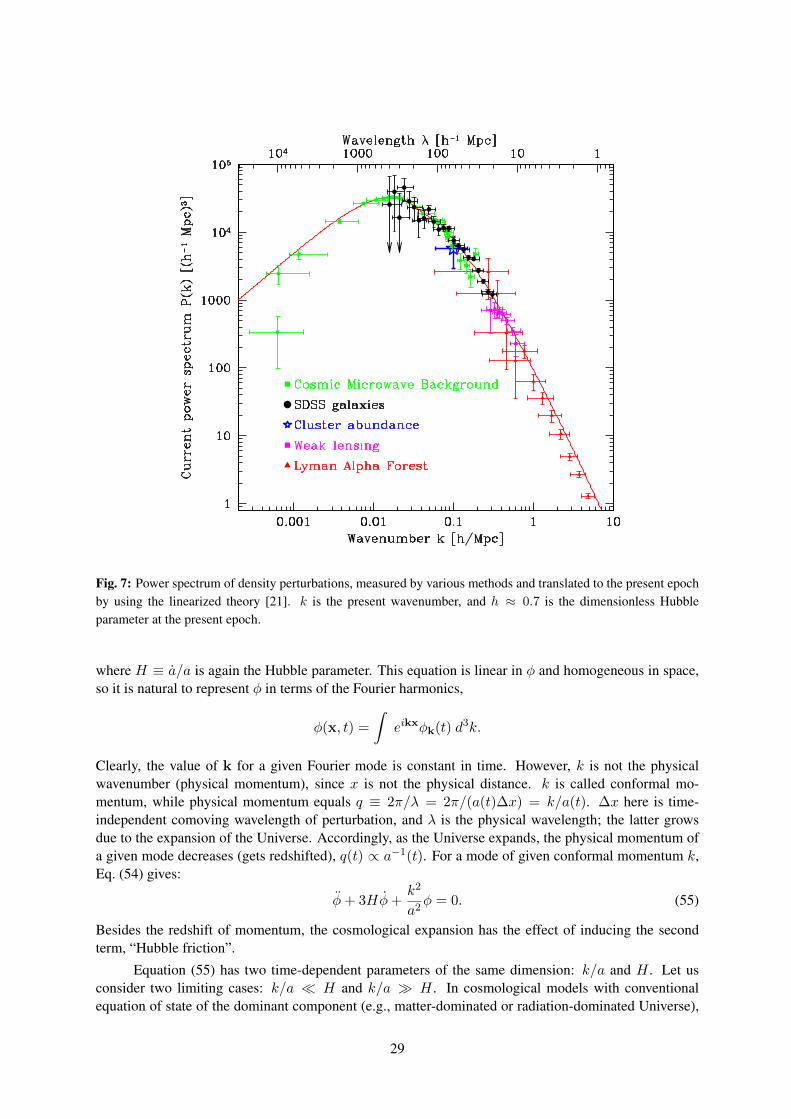
Fig. 7: Power spectrum of density perturbations, measured by various methods and translated to the present epochby using the linearized theory [21]. k is the present wavenumber, and h ≈ 0.7 is the dimensionless Hubbleparameter at the present epoch.

where H ≡ a/a is again the Hubble parameter. This equation is linear in φ and homogeneous in space,so it is natural to represent φ in terms of the Fourier harmonics,

φ(x, t) =

∫eikxφk(t) d3k.

Clearly, the value of k for a given Fourier mode is constant in time. However, k is not the physicalwavenumber (physical momentum), since x is not the physical distance. k is called conformal mo-mentum, while physical momentum equals q ≡ 2π/λ = 2π/(a(t)∆x) = k/a(t). ∆x here is time-independent comoving wavelength of perturbation, and λ is the physical wavelength; the latter growsdue to the expansion of the Universe. Accordingly, as the Universe expands, the physical momentum ofa given mode decreases (gets redshifted), q(t) ∝ a−1(t). For a mode of given conformal momentum k,Eq. (54) gives:

φ+ 3Hφ+k2

a2φ = 0. (55)

Besides the redshift of momentum, the cosmological expansion has the effect of inducing the secondterm, “Hubble friction”.

Equation (55) has two time-dependent parameters of the same dimension: k/a and H . Let usconsider two limiting cases: k/a H and k/a H . In cosmological models with conventionalequation of state of the dominant component (e.g., matter-dominated or radiation-dominated Universe),

29

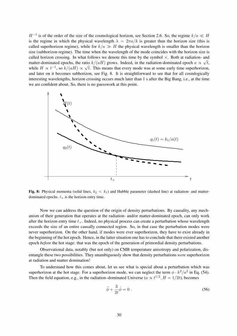
H−1 is of the order of the size of the cosmological horizon, see Section 2.6. So, the regime k/a His the regime in which the physical wavelength λ = 2πa/k is greater than the horizon size (this iscalled superhorizon regime), while for k/a H the physical wavelength is smaller than the horizonsize (subhorizon regime). The time when the wavelength of the mode coincides with the horizon size iscalled horizon crossing. In what follows we denote this time by the symbol ×. Both at radiation- andmatter-dominated epochs, the ratio k/(aH) grows. Indeed, in the radiation-dominated epoch a ∝

√t,

while H ∝ t−1, so k/(aH) ∝√t. This means that every mode was at some early time superhorizon,

and later on it becomes subhorizon, see Fig. 8. It is straightforward to see that for all cosmlogicallyinteresting wavelengths, horizon crossing occurs much later than 1 s after the Big Bang, i.e., at the timewe are confident about. So, there is no guesswork at this point.

t

q2(t)

q1(t) = k1/a(t)

H(t)

t×

Fig. 8: Physical momenta (solid lines, k2 < k1) and Hubble parameter (dashed line) at radiation- and matter-dominated epochs. t× is the horizon entry time.

Now we can address the question of the origin of density perturbations. By causality, any mech-anism of their generation that operates at the radiation- and/or matter-dominated epoch, can only workafter the horizon entry time t×. Indeed, no physical process can create a perturbation whose wavelengthexceeds the size of an entire causally connected region. So, in that case the perturbation modes werenever superhorizon. On the other hand, if modes were ever superhorizon, they have to exist already inthe beginning of the hot epoch. Hence, in the latter situation one has to conclude that there existed anotherepoch before the hot stage: that was the epoch of the generation of primordial density perturbations.

Observational data, notably (but not only) on CMB temperature anisotropy and polarization, dis-entangle these two possibilities. They unambiguously show that density perturbations were superhorizonat radiation and matter domination!

To understand how this comes about, let us see what is special about a perturbation which wassuperhorizon at the hot stage. For a superhorizon mode, we can neglect the term φ · k2/a2 in Eq. (54).Then the field equation, e.g., in the radiation–dominated Universe (a ∝ t1/2, H = 1/2t), becomes

φ+3

2tφ = 0 . (56)

30

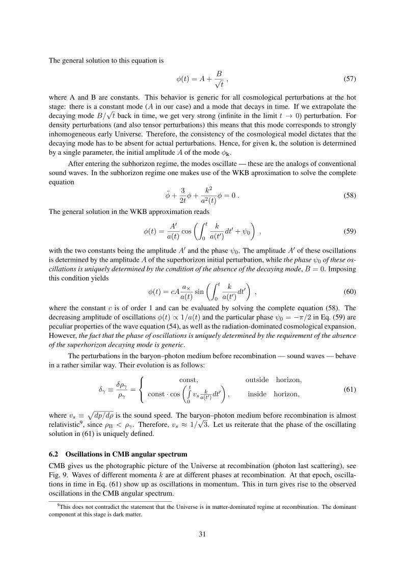
The general solution to this equation is

φ(t) = A+B√t, (57)

where A and B are constants. This behavior is generic for all cosmological perturbations at the hotstage: there is a constant mode (A in our case) and a mode that decays in time. If we extrapolate thedecaying mode B/

√t back in time, we get very strong (infinite in the limit t → 0) perturbation. For

density perturbations (and also tensor perturbations) this means that this mode corresponds to stronglyinhomogeneous early Universe. Therefore, the consistency of the cosmological model dictates that thedecaying mode has to be absent for actual perturbations. Hence, for given k, the solution is determinedby a single parameter, the initial amplitude A of the mode φk.

After entering the subhorizon regime, the modes oscillate — these are the analogs of conventionalsound waves. In the subhorizon regime one makes use of the WKB aproximation to solve the completeequation

φ+3

2tφ+

k2

a2(t)φ = 0 . (58)

The general solution in the WKB approximation reads

φ(t) =A′

a(t)cos

(∫ t

0

k

a(t′)dt′ + ψ0

), (59)

with the two constants being the amplitude A′ and the phase ψ0. The amplitude A′ of these oscillationsis determined by the amplitudeA of the superhorizon initial perturbation, while the phase ψ0 of these os-cillations is uniquely determined by the condition of the absence of the decaying mode, B = 0. Imposingthis condition yields

φ(t) = cAa×a(t)

sin

(∫ t

0

k

a(t′)dt′), (60)

where the constant c is of order 1 and can be evaluated by solving the complete equation (58). Thedecreasing amplitude of oscillations φ(t) ∝ 1/a(t) and the particular phase ψ0 = −π/2 in Eq. (59) arepeculiar properties of the wave equation (54), as well as the radiation-dominated cosmological expansion.However, the fact that the phase of oscillations is uniquely determined by the requirement of the absenceof the superhorizon decaying mode is generic.

The perturbations in the baryon–photon medium before recombination — sound waves — behavein a rather similar way. Their evolution is as follows:

δγ ≡δργργ

=

const, outside horizon,

const · cos

(t∫

0

vsk

a(t′)dt′), inside horizon,

(61)

where vs ≡√dp/dρ is the sound speed. The baryon–photon medium before recombination is almost

relativistic9, since ρB < ργ . Therefore, vs ≈ 1/√

3. Let us reiterate that the phase of the oscillatingsolution in (61) is uniquely defined.

6.2 Oscillations in CMB angular spectrumCMB gives us the photographic picture of the Universe at recombination (photon last scattering), seeFig. 9. Waves of different momenta k are at different phases at recombination. At that epoch, oscilla-tions in time in Eq. (61) show up as oscillations in momentum. This in turn gives rise to the observedoscillations in the CMB angular spectrum.

9This does not contradict the statement that the Universe is in matter-dominated regime at recombination. The dominantcomponent at this stage is dark matter.

31

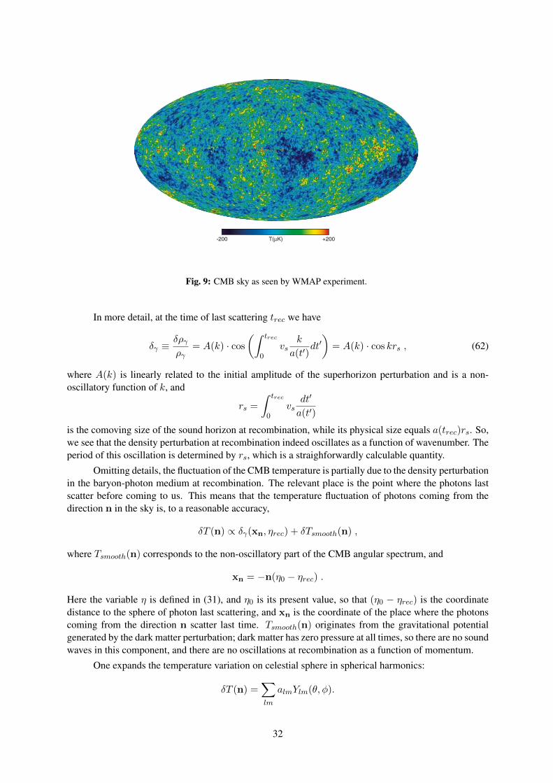
this condition yields

!(t) = cAa!a(t)

sin

!" t

0

k

a(t")dt"

#, (60)

where the constant c is of order 1 and can be evaluated by solving the com-plete equation (58). The decreasing amplitude of oscillations !(t) ! 1/a(t)and the particular phase "0 = "#/2 in (59) are peculiar properties of thewave equation (54), as well as the radiation-dominated cosmological expan-sion. However, the fact that the phase of oscillations is uniquely determined bythe requirement of the absence of the superhorizon decaying mode is generic.

The perturbations in the baryon–photon medium before recombination — soundwaves — behave in a rather similar way. Their evolution is as follows:

$! #$%!

%!=

$%&

const, outside horizon,

const · cos!

t'0

vsk

a(t!)dt"#

, inside horizon,(61)

where vs #(

dp/d% is the sound speed. The baryon–photon medium beforerecombination is almost relativistic9, since %B < %! . Therefore, vs $ 1/

%3.

Let us reiterate that the phase of the oscillating solution in (61) is uniquelydefined.

6.2 Oscillations in CMB angular spectrumCMB gives us the photographic picture of the Universe at recombination (pho-ton last scattering), see Fig. 9. Waves of different momenta k are at differentphases at recombination. At that epoch, oscillations in time in Eq. (61) showup as oscillations in momentum. This in turn gives rise to the observed oscil-lations in the CMB angular spectrum.

Fig. 9: CMB sky as seen by WMAP experiment.

9This does not contradict the statement that the Universe is in matter-dominated regime at recombination. The dominantcomponent at this stage is dark matter.

37

Fig. 9: CMB sky as seen by WMAP experiment.

In more detail, at the time of last scattering trec we have

δγ ≡δργργ

= A(k) · cos

(∫ trec

0vs

k

a(t′)dt′)

= A(k) · cos krs , (62)

where A(k) is linearly related to the initial amplitude of the superhorizon perturbation and is a non-oscillatory function of k, and

rs =

∫ trec

0vs

dt′

a(t′)

is the comoving size of the sound horizon at recombination, while its physical size equals a(trec)rs. So,we see that the density perturbation at recombination indeed oscillates as a function of wavenumber. Theperiod of this oscillation is determined by rs, which is a straighforwardly calculable quantity.

Omitting details, the fluctuation of the CMB temperature is partially due to the density perturbationin the baryon-photon medium at recombination. The relevant place is the point where the photons lastscatter before coming to us. This means that the temperature fluctuation of photons coming from thedirection n in the sky is, to a reasonable accuracy,

δT (n) ∝ δγ(xn, ηrec) + δTsmooth(n) ,

where Tsmooth(n) corresponds to the non-oscillatory part of the CMB angular spectrum, and

xn = −n(η0 − ηrec) .

Here the variable η is defined in (31), and η0 is its present value, so that (η0 − ηrec) is the coordinatedistance to the sphere of photon last scattering, and xn is the coordinate of the place where the photonscoming from the direction n scatter last time. Tsmooth(n) originates from the gravitational potentialgenerated by the dark matter perturbation; dark matter has zero pressure at all times, so there are no soundwaves in this component, and there are no oscillations at recombination as a function of momentum.

One expands the temperature variation on celestial sphere in spherical harmonics:

δT (n) =∑

lm

almYlm(θ, φ).

32

The multipole number l characterizes the temperature fluctuations at the angular scale ∆θ = π/l. Thesound waves of momentum k are seen roughly at an angle ∆θ = ∆x/(η0 − ηrec), where ∆x = π/k iscoordinate half-wavelength. Hence, there is the correspondence

l←→ k(η0 − ηrec) .

Oscillations in momenta in (62) thus translate into oscillations in l, and these are indeed observed, seeFig. 10.

Fig. 10: The angular spectrum of the CMB temperature anisotropy [22]. The quantity in vertical axis is Dl definedin Eq. (65).

To understand what is shown in Fig. 10, we note that all observations today support the hypothesisthat alm are independent Gaussian random variables. Gaussianity means that

P (alm)dalm =1√

2πCle−a

2lm

2Cl dalm, (63)

where P (alm) is the probability density for the random variable alm. For a hypothetical ensemble ofUniverses like ours, the average values of products of the coefficients alm would obey

〈almal′m′〉 = Clδll′δmm′ . (64)

This gives the expression for the temperature fluctuation:

〈[δT (n)]2〉 =∑

l

2l + 1

4πCl ≈

∫dl

lDl ,

where

Dl =l(l + 1)

2πCl . (65)

It is the latter quantity that is usually shown in plots, in particular, in Fig. 10. Note the unconventionalscale on the horizontal axis, aimed at showing both small l region (large angular scales) and large lregion.

The fact that the CMB angular spectrum has oscillatory behavior unambiguously tells us thatdensity perturbations were indeed superhorizon at hot cosmological stage. If these perturbations were

33

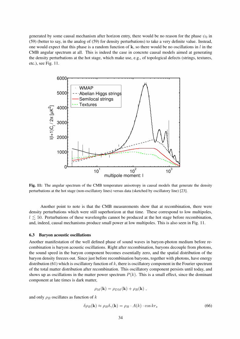
generated by some causal mechanism after horizon entry, there would be no reason for the phase ψ0 in(59) (better to say, in the analog of (59) for density perturbations) to take a very definite value. Instead,one would expect that this phase is a random function of k, so there would be no oscillations in l in theCMB angular spectrum at all. This is indeed the case in concrete causal models aimed at generatingthe density perturbations at the hot stage, which make use, e.g., of topological defects (strings, textures,etc.), see Fig. 11.

101

102

103

0

1000

2000

3000

4000

5000

6000

multipole moment: l

l(l+

1)C

l / 2

π [

µK

2]

WMAP

Abelian Higgs strings

Semilocal strings

Textures

Fig. 11: The angular spectrum of the CMB temperature anisotropy in causal models that generate the densityperturbations at the hot stage (non-oscillatory lines) versus data (sketched by oscillatory line) [23].

Another point to note is that the CMB measurements show that at recombination, there weredensity perturbations which were still superhorizon at that time. These correspond to low multipoles,l . 50. Perturbations of these wavelengths cannot be produced at the hot stage before recombination,and, indeed, causal mechanisms produce small power at low multipoles. This is also seen in Fig. 11.

6.3 Baryon acoustic oscillationsAnother manifestation of the well defined phase of sound waves in baryon-photon medium before re-combination is baryon acoustic oscillations. Right after recombination, baryons decouple from photons,the sound speed in the baryon component becomes essentially zero, and the spatial distribution of thebaryon density freezes out. Since just before recombination baryons, together with photons, have energydistribution (61) which is oscillatory function of k, there is oscillatory component in the Fourier spectrumof the total matter distribution after recombination. This oscillatory component persists until today, andshows up as oscillations in the matter power spectrum P (k). This is a small effect, since the dominantcomponent at late times is dark matter,

ρM (k) = ρDM (k) + ρB(k) ,

and only ρB oscillates as function of k

δρB(k) ≈ ρBδγ(k) = ρB ·A(k) · cos krs (66)

34

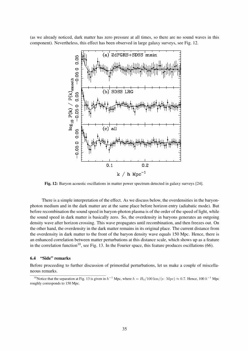
(as we already noticed, dark matter has zero pressure at all times, so there are no sound waves in thiscomponent). Nevertheless, this effect has been observed in large galaxy surveys, see Fig. 12.

Fig. 12: Baryon acoustic oscillations in matter power spectrum detected in galaxy surveys [24].

There is a simple interpretation of the effect. As we discuss below, the overdensities in the baryon-photon medium and in the dark matter are at the same place before horizon entry (adiabatic mode). Butbefore recombination the sound speed in baryon-photon plasma is of the order of the speed of light, whilethe sound speed in dark matter is basically zero. So, the overdensity in baryons generates an outgoingdensity wave after horizon crossing. This wave propagates until recombination, and then freezes out. Onthe other hand, the overdensity in the dark matter remains in its original place. The current distance fromthe overdensity in dark matter to the front of the baryon density wave equals 150 Mpc. Hence, there isan enhanced correlation between matter perturbations at this distance scale, which shows up as a featurein the correlation function10, see Fig. 13. In the Fourier space, this feature produces oscillations (66).

6.4 “Side” remarksBefore proceeding to further discussion of primordial perturbations, let us make a couple of miscella-neous remarks.

10Notice that the separation at Fig. 13 is given in h−1 Mpc, where h = H0/100 km/(s ·Mpc) ≈ 0.7. Hence, 100 h−1 Mpcroughly corresponds to 150 Mpc.

35

Fig. 13: Baryon acoustic oscillations in galaxy correlation function [25].

6.4.1 Cosmic variance.We can measure only one Universe, and the best one can do is to define the angular spectrum Cl obtainedfrom the data as

Cl =1

2l + 1

l∑

m=−l|alm|2 .

This is not the same thing as Cl defined in (64), as the latter definition involves averaging over anensemble of Universes. For given l, there are (2l+1) independent coefficients alm only, so there exists anirreducible statistical uncertainty of order δCl/Cl ∼ 1/

√2l + 1, called cosmic variance. It is particularly

pronounced at small l and, indeed, it is much larger than the experimental errors in this part of the angularspectrum (as an example, error bars in the left part of Fig. 10 are precisely due to the cosmic variance).

6.4.2 Measuring the cosmological parameters.The angular spectrum of CMB temperature anisotropy and polarization, as well as other cosmologicaldata, encodes information on the cosmological parameters. As an example, the sound horizon at recom-bination is a good standard ruler back at that epoch. It is seen at an angle that depends on the geometryof 3-dimensional space (an interval is seen at larger angle on a sphere than on a plane) and on the darkenergy density (since dark energy affects the distance to the sphere of photon last scattering). This isshown in Fig. 14.

Likewise, the baryon acoustic oscillations provide a standard ruler at relatively late times (lowredshifts z ∼ 0.2 − 0.4). A combination of their measurement with CMB anisotropy give quite precisedetermination of both spatial curvature (which is found to be zero within error bars) and dark energydensity. Notably, this determination of ρΛ is in good agreement with various independent data, notably,with the data on SNe 1a, which were the first unambiguous evidence for dark energy [27, 28].

There are many other ways in which the cosmological parameters, including ΩB and ΩDM , affect

36

Fig. 14: Effect of spatial curvature (left) and dark energy (right) on the CMB temperature angular spectrum [26].Ωk = ±(RH0)2 is the relative contribution of spatial curvature to the Friedmann equation, withR being the radiusof spatial curvature. Negative sign corresponds to 3-sphere. As Ωk decreases, the curves in the left plot move left.Likewise, the curves on the right plot move left as ΩΛ increases.

the CMB anisotropies. In particular, the hights of the acoustic peaks in the CMB temperature angularspectrum are very sensitive to the baryon-to-photon ratio ηB (and hence to ΩB), the overall shape of thecurve in Fig. 10 stronfly depends on ΩDM , etc. By fitting the CMB data and combining them with theresults of other cosmological observations, one is able to obtain quite precise knowledge of our Universe.

6.5 Properties of primordial density perturbations — hints about the earliest cosmological epochAs we emphasized above, the density perturbations were generated at a very early, pre-hot epoch of thecosmological evolution. Obviously, it is of fundamental importance to figure out what precisely thatepoch was. One of its properties is clear right away: it must be such that the cosmologically relevantwavelengths, including the wavelengths of the present horizon scale, were subhorizon early at that epoch.Only in that case the perturbations of these wavelengths could be generated in a causal manner at thepre-hot epoch. Notice that this is another manifestation of the horizon problem discussed in Section 2.6:we know from the observational data on density perturbtions that our entire visible Universe was causallyconnected by the beginning of the hot stage.

An excellent hypothesis on the pre-hot stage is inflation, the epoch of nearly exponential expan-sion,

a(t) = e∫Hdt , H ≈ const .

Originally [29], inflation was designed to solve the problems of the hot Big Bang cosmology, such asthe horizon problem, as well as the flatness, entropy and other problems. It does this job very well: thehorizon size at inflation is at least

lH(t) = a(t)

∫ t

ti

dt′

a(t′)= H−1eH(t−ti) ,

where ti is the time inflation begins, and we set H = const for illustrational purposes. This size is hugefor t− ti H−1, so the entire visible Universe is naturally causally connected.

From the viewpoint of perturbations, the physical momentum q(t) = k/a(t) decreases (gets red-shifted) at inflation, while the Hubble parameter stays almost constant. So, every mode is first subhorizon(q(t) H(t)), and later superhorizon (q(t) H(t)) at inflation. This situation is opposite to what hap-pens at radiation and matter domination, see Fig. 15; this is precisely the pre-requisite for generatingthe density perturbations. In fact, inflation does generate primordial density perturbations [30], whoseproperties are consistent with everything we know about them.

37

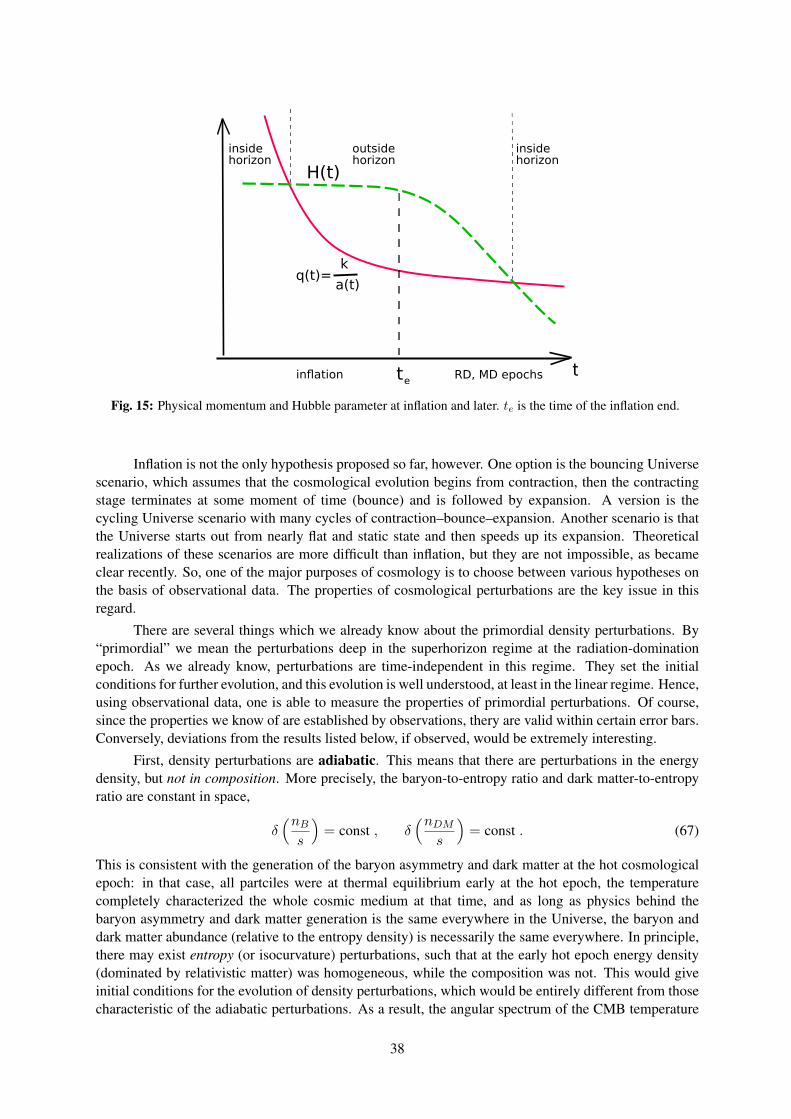
inflation RD, MD epochs

H(t)

q(t)=a(t)

k

tte

insidehorizon

insidehorizon

outsidehorizon

Fig. 15: Physical momentum and Hubble parameter at inflation and later. te is the time of the inflation end.

Inflation is not the only hypothesis proposed so far, however. One option is the bouncing Universescenario, which assumes that the cosmological evolution begins from contraction, then the contractingstage terminates at some moment of time (bounce) and is followed by expansion. A version is thecycling Universe scenario with many cycles of contraction–bounce–expansion. Another scenario is thatthe Universe starts out from nearly flat and static state and then speeds up its expansion. Theoreticalrealizations of these scenarios are more difficult than inflation, but they are not impossible, as becameclear recently. So, one of the major purposes of cosmology is to choose between various hypotheses onthe basis of observational data. The properties of cosmological perturbations are the key issue in thisregard.

There are several things which we already know about the primordial density perturbations. By“primordial” we mean the perturbations deep in the superhorizon regime at the radiation-dominationepoch. As we already know, perturbations are time-independent in this regime. They set the initialconditions for further evolution, and this evolution is well understood, at least in the linear regime. Hence,using observational data, one is able to measure the properties of primordial perturbations. Of course,since the properties we know of are established by observations, thery are valid within certain error bars.Conversely, deviations from the results listed below, if observed, would be extremely interesting.

First, density perturbations are adiabatic. This means that there are perturbations in the energydensity, but not in composition. More precisely, the baryon-to-entropy ratio and dark matter-to-entropyratio are constant in space,

δ(nBs

)= const , δ

(nDMs

)= const . (67)

This is consistent with the generation of the baryon asymmetry and dark matter at the hot cosmologicalepoch: in that case, all partciles were at thermal equilibrium early at the hot epoch, the temperaturecompletely characterized the whole cosmic medium at that time, and as long as physics behind thebaryon asymmetry and dark matter generation is the same everywhere in the Universe, the baryon anddark matter abundance (relative to the entropy density) is necessarily the same everywhere. In principle,there may exist entropy (or isocurvature) perturbations, such that at the early hot epoch energy density(dominated by relativistic matter) was homogeneous, while the composition was not. This would giveinitial conditions for the evolution of density perturbations, which would be entirely different from thosecharacteristic of the adiabatic perturbations. As a result, the angular spectrum of the CMB temperature

38

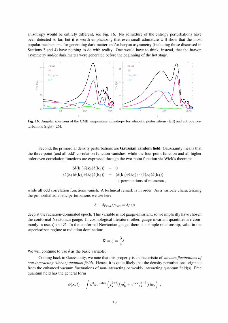
anisotropy would be entirely different, see Fig. 16. No admixture of the entropy perturbations havebeen detected so far, but it is worth emphasizing that even small admixture will show that the mostpopular mechanisms for generating dark matter and/or baryon asymmetry (including those discussed inSections 3 and 4) have nothing to do with reality. One would have to think, instead, that the baryonasymmetry and/or dark matter were generated before the beginning of the hot stage.

Fig. 16: Angular spectrum of the CMB temperature anisotropy for adiabatic perturbations (left) and entropy per-turbations (right) [26].

Second, the primordial density perturbations are Gaussian random field. Gaussianity means thatthe three-point (and all odd) correlation function vanishes, while the four-point function and all higherorder even correlation functions are expressed through the two-point function via Wick’s theorem:

〈δ(k1)δ(k2)δ(k3)〉 = 0

〈δ(k1)δ(k2)δ(k3)δ(k4)〉 = 〈δ(k1)δ(k2)〉 · 〈δ(k3)δ(k4)〉+ permutations of momenta ,

while all odd correlation functions vanish. A technical remark is in order. As a varibale characterizingthe primordial adiabatic perturbations we use here

δ ≡ δρrad/ρrad = δρ/ρ

deep at the radiation-dominated epoch. This variable is not gauge-invariant, so we implicitly have chosenthe conformal Newtonian gauge. In cosmological literature, other, gauge-invariant quantities are com-monly in use, ζ and R. In the conformal Newtonian gauge, there is a simple relationship, valid in thesuperhorizon regime at radiation domination:

R = ζ =3

4δ .

We will continue to use δ as the basic variable.

Coming back to Gaussianity, we note that this property is characteristic of vacuum fluctuations ofnon-interacting (linear) quantum fields. Hence, it is quite likely that the density perturbations originatefrom the enhanced vacuum fluctuations of non-interacting or weakly interacting quantum field(s). Freequantum field has the general form

φ(x, t) =

∫d3ke−ikx

(f

(+)k (t)a†k + eikxf

(−)k (t)ak

),

39

where a†k and ak are creation and annihilation operators. For the field in Minkowski space-time one hasf

(±)k (t) = e±iωkt, while enhancement, e.g. due to the evolution in time-dependent background, means

that f (±)k are large. But in any case, Wick’s theorem is valid, provided that the state of the system is

vacuum, ak|0〉 = 0.

Inflation does the job very well: fluctuations of all light fields get enhanced greatly due to the fastexpansion of the Universe. This is true, in particular, for the field that dominates the energy density atinflation, called inflaton. Enhanced vacuum fluctuations of the inflaton are nothing but perturbations inthe energy density at inflationary epoch in the simplest inflationary models, which are reprocessed intoperturbations in the hot medium after the end of inflation. The generation of the density perturbations isless automatic in scenarios alternative to inflation, but there are various examples showing that this is nota particularly difficult problem.

Non-Gaussianity is an important topic of current research. It would show up as a deviation fromWick’s theorem. As an example, the three-point function (bispectrum) may be non-vanishing,

〈δ(k1)δ(k2)δ(k3)〉 = δ(k1 + k2 + k3) G(k2i ; k1k2; k1k3) 6= 0 .

The shape of G(k2i ; k1k2; k1k3) is different in different models, so this shape is a potential discrim-

inator. In some models the bispectrum vanishes, e.g., due to symmetries. In that case the trispectrum(connected 4-point function) may be measurable instead. Non-Gaussianity is very small in the simplestinflationary models, but it can be sizeable in more contrived models of inflation and in alternatives toinflation. It is worth emphasizing that non-Gaussianity has not been detected yet.

Another important property is that the primordial power spectrum of density perturbations is flat(or almost flat). A convenient definition of the power spectrum for homogeneous and anisotropic Gaus-sian random field is11

〈δ(k)δ(k′)〉 =1

4πk3P(k)δ(k + k′) . (68)

The power spectrum P(k) defined in this way determines the fluctuation in a logarithmic interval ofmomenta,

〈δ2(x)〉 =

∫ ∞

0

dk

kP(k) .

By definition, the flat spectrum is such that P is independent of k. It is worth noting that the flat spectrumwas conjectured by E. Harrison [31] and Ya. Zeldovich [32] in the beginning of 1970’s, long beforerealistic mechanisms of the generation of density perturbations have been proposed.

In view of the approximate flatness, a natural parametrization is

P(k) = As

(k

k∗

)ns−1

, (69)

whereAs is the amplitude, (ns−1) is the tilt and k∗ is a fiducial momentum, chosen at one’s convenience.The flat spectrum in this parametrization has ns = 1. Cosmological data favor the value ns ≈ 0.96 (i.e.,slightly smaller than 1), see below, but it is fair to say that ns = 1 is still consistent with observations.

The flatness of the power spectrum calls for some symmetry behind this property. In inflationarytheory this is the symmetry of the de Sitter space-time, which is the space time of constant Hubble rate,

ds2 = dt2 − e2Htdx2 , H = const .

This metric is invariant under spatial dilatations supplemented by time translations,

x→ λx , t→ t− 1

2Hlog λ .

11Note that the the definition of the power spectrum used in Figs. 7 and 12 is different from (68).

40

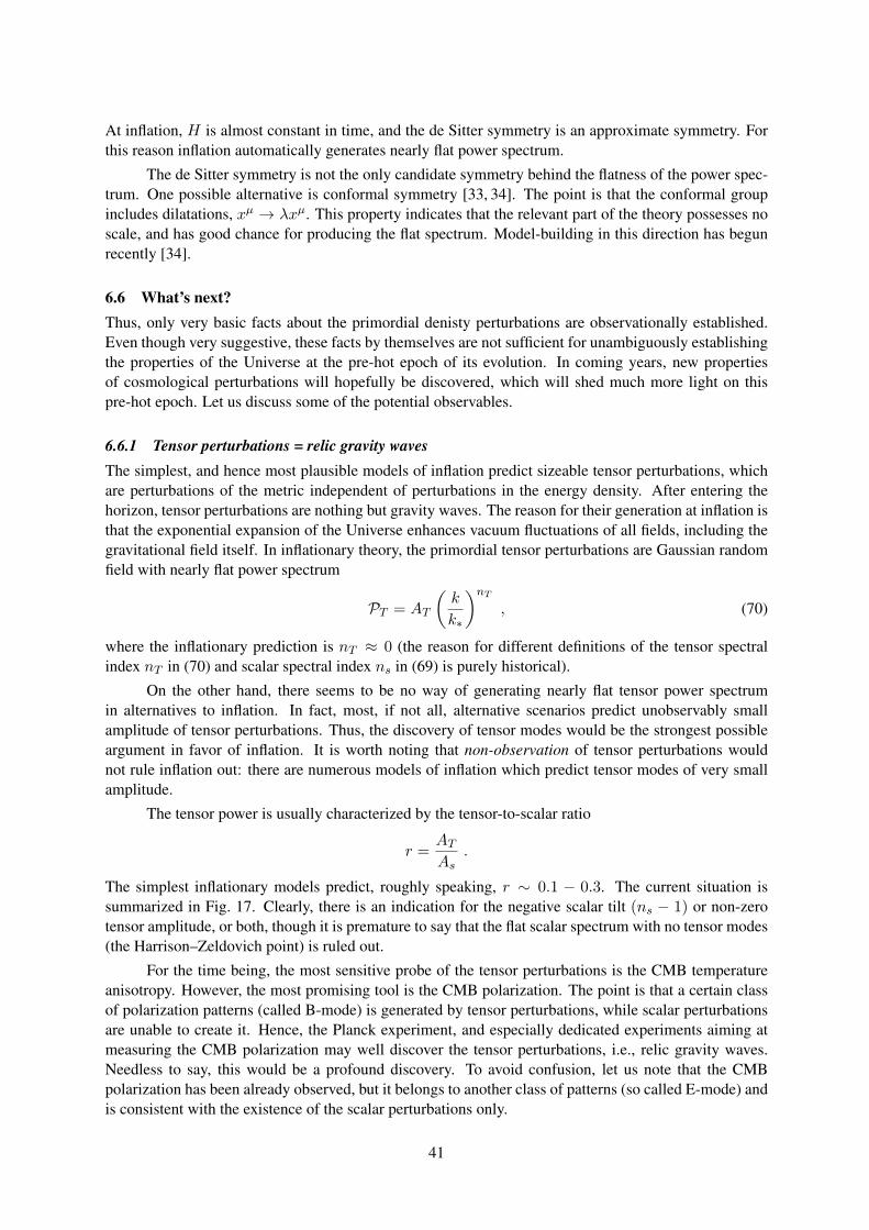
At inflation, H is almost constant in time, and the de Sitter symmetry is an approximate symmetry. Forthis reason inflation automatically generates nearly flat power spectrum.

The de Sitter symmetry is not the only candidate symmetry behind the flatness of the power spec-trum. One possible alternative is conformal symmetry [33, 34]. The point is that the conformal groupincludes dilatations, xµ → λxµ. This property indicates that the relevant part of the theory possesses noscale, and has good chance for producing the flat spectrum. Model-building in this direction has begunrecently [34].

6.6 What’s next?Thus, only very basic facts about the primordial denisty perturbations are observationally established.Even though very suggestive, these facts by themselves are not sufficient for unambiguously establishingthe properties of the Universe at the pre-hot epoch of its evolution. In coming years, new propertiesof cosmological perturbations will hopefully be discovered, which will shed much more light on thispre-hot epoch. Let us discuss some of the potential observables.

6.6.1 Tensor perturbations = relic gravity wavesThe simplest, and hence most plausible models of inflation predict sizeable tensor perturbations, whichare perturbations of the metric independent of perturbations in the energy density. After entering thehorizon, tensor perturbations are nothing but gravity waves. The reason for their generation at inflation isthat the exponential expansion of the Universe enhances vacuum fluctuations of all fields, including thegravitational field itself. In inflationary theory, the primordial tensor perturbations are Gaussian randomfield with nearly flat power spectrum

PT = AT

(k

k∗

)nT, (70)

where the inflationary prediction is nT ≈ 0 (the reason for different definitions of the tensor spectralindex nT in (70) and scalar spectral index ns in (69) is purely historical).

On the other hand, there seems to be no way of generating nearly flat tensor power spectrumin alternatives to inflation. In fact, most, if not all, alternative scenarios predict unobservably smallamplitude of tensor perturbations. Thus, the discovery of tensor modes would be the strongest possibleargument in favor of inflation. It is worth noting that non-observation of tensor perturbations wouldnot rule inflation out: there are numerous models of inflation which predict tensor modes of very smallamplitude.

The tensor power is usually characterized by the tensor-to-scalar ratio

r =ATAs

.

The simplest inflationary models predict, roughly speaking, r ∼ 0.1 − 0.3. The current situation issummarized in Fig. 17. Clearly, there is an indication for the negative scalar tilt (ns − 1) or non-zerotensor amplitude, or both, though it is premature to say that the flat scalar spectrum with no tensor modes(the Harrison–Zeldovich point) is ruled out.

For the time being, the most sensitive probe of the tensor perturbations is the CMB temperatureanisotropy. However, the most promising tool is the CMB polarization. The point is that a certain classof polarization patterns (called B-mode) is generated by tensor perturbations, while scalar perturbationsare unable to create it. Hence, the Planck experiment, and especially dedicated experiments aiming atmeasuring the CMB polarization may well discover the tensor perturbations, i.e., relic gravity waves.Needless to say, this would be a profound discovery. To avoid confusion, let us note that the CMBpolarization has been already observed, but it belongs to another class of patterns (so called E-mode) andis consistent with the existence of the scalar perturbations only.

41

Fig. 17: Allowed regions (at 68% and 95% CL) in the plane (ns, r), where ns is the scalar spectral index and r isthe tensor-to-scalar ratio. Rectangle shows the Harrison–Zeldovich point (flat scalar spectrum, no tensor modes).Points on the lines show predictions of popular inflationary models.

6.6.2 Scalar tilt.Inflationary models and their alternatives will be constrained by the precise determination of the scalartilt (ns − 1) and its dependence on momentum k. It appears, however, that the information on ns(k)that will be obtained in reasonably near future will be of limited significance from the viewpoint ofdiscriminating between different (and even grossly different) scenarios.

6.6.3 Non-Gaussianity.As we pointed out already, non-Gaussianity of density perturbations is very small in the simplest infla-tionary models. Hence, its discovery will signalize that either inflation and inflationary generation ofdensity perturbations occured in a rather complicated way, or an alternative scenario was realized. Oncethe non-Gaussianity is discovered, and its shape is revealed even with moderate accuracy, many concretemodels will be ruled out, while at most a few will get strong support.

6.6.4 Statistical anisotropy.In principle, the power spectrum of density perturbations may depend on the direction of momentum,e.g.,

P(k) = P0(k)

(1 + wij(k)

kikjk2

+ . . .

)

where wij is a fundamental tensor in our part of the Universe (odd powers of ki would contradict com-mutativity of the Gaussian random field δ(k), see Eq. (68)). Such a dependence would definitely implythat the Universe was anisotropic at the pre-hot stage, when the primordial perturbations were generated.This statistical anisotropy is rather hard to obtain in inflationary models, though it is possible in inflationwith strong vector fields [35]. On the other hand, statistical anisotropy is natural in some other scenarios,including conformal models [36]

The statistical anisotropy would show up in correlators [37]

〈almal′m′〉 with l′ 6= l and/or m′ 6= m

At the moment, the situation with observational data is controversial [38], and the new data, notably fromthe Planck experiment, will hopefully clear it up.

42

6.6.5 Admixture of entropy perturbations.As we explained above, even small admixture of entropy perturbations would force us to abandon themost popular scenarios of the generation of baryon asymmetry and/or dark matter, which assumed thatit happened at the hot epoch. The WIMP dark matter would no longer be well motivated, while other,very weakly interacting dark matter candidates, like axion or superheavy relic, would be prefered. Thiswould make the direct searches for dark matter rather problematic.

7 ConclusionWe are at the eve of new era not only in particles physics, but also in cosmology. There is reasonablywell justified expectation that the LHC will shed light on long-standing cosmological problems of theorigin of the baryon asymmetry and nature of dark matter in our Universe. The ideas we discussed inthese lectures in this regard may well be not the right ones: we can only hypothesize on physics beyondthe Standard Model and its role in the early Universe.

In fact, the TeV scale physics may be dramatically different from physics we get used to. As anexample, it is not excluded that TeV is not only electroweak, but also gravitational scale. This is the casein models with large extra dimensions, in which the Planck scale is related to the fundamental gravityscale in a way that involves the volume of extra dimensions, and hence the fundamental scale can bemuch below MPl (for a review see, e.g., Ref. [39]). If the LHC will find that, indeed, the fundamentalgravity scale is in the TeV range, this would have most profound consequences for both microscopicphysics and cosmology. On the microscopic physics side, this would enable one to study at collidersquantum gravity and its high-energy extension — possibly string theory, while on the cosmological side,the entire picture of the early Universe would have to be revised. Inflation, if any, would have to occureither at low energy density or in the regime of strong quantum gravity effects. The highest temperaturesin the usual expansion history would be at most in the TeV range, so dark matter and baryon asymmetrywould have to be generated either below TeV temperatures or in quantum gravity regime. Even moreintriguing will be the study of quantum gravity cosmological epoch, with hints from colliders graduallycoming. This, probably, is too bright a prospective to be realistic.

It is more likely that the LHC will find something entirely new, something theorists have notthought about. Or, conversely, find so little that one will have to get serious about anthropic principle.In any case, the LHC results will definitely change the landscape of fundamental physics, cosmologyincluded.

The observational data unequivocally tell us that the hot stage of the cosmological evolution waspreceeded by some other epoch, at which the cosmological perturbations were generated. The bestguess for this epoch is inflation, but one should bear in mind that there are alternative possibilities. Itis fascinating that with new observational data, there is good chance to learn what precisely that pre-hotepoch was. It may very well be that in this way we will be able to probe physics at the energy, distanceand time scales well beyond the reach of the LHC.

References[1] R. H. Brandenberger, Particle physics aspects of modern cosmology, arXiv:hep-ph/9701276;

W. L. Freedman and M. S. Turner, Rev. Mod. Phys. 75 (2003) 1433 [arXiv:astro-ph/0308418];V. Rubakov, PoS RTN2005 (2005) 003; J. A. Peacock, Cosmology and particle physics, in Proc.1998 European School of High-Energy Physics, St. Andrews, Scotland; M. Shaposhnikov, Cosmol-ogy and astrophysics, in Proc. 2000 European School of High-Energy Physics, Caramulo, Portu-gal; I. I. Tkachev, Astroparticle physics, in Proc. 2003 European School on High-Energy Physics,Tsakhkadzor, Armenia, arXiv:hep-ph/0405168.

[2] G. Jungman, M. Kamionkowski and K. Griest, Phys. Rept. 267 (1996) 195 [arXiv:hep-ph/9506380]; A. Bottino and N. Fornengo, Dark matter and its particle candidates, arXiv:hep-

43

ph/9904469; K. A. Olive, Dark matter, arXiv:astro-ph/0301505; G. Bertone, D. Hooper and J. Silk,Phys. Rept. 405 (2005) 279. [arXiv:hep-ph/0404175].

[3] A. D. Dolgov, Baryogenesis, 30 years after, arXiv:hep-ph/9707419 V. A. Rubakov and M. E. Sha-poshnikov, Usp. Fiz. Nauk 166 (1996) 493 [Phys. Usp. 39 (1996) 461] [arXiv:hep-ph/9603208];A. Riotto and M. Trodden, Ann. Rev. Nucl. Part. Sci. 49 (1999) 35 [arXiv:hep-ph/9901362];M. Trodden, Rev. Mod. Phys. 71 (1999) 1463 [arXiv:hep-ph/9803479].

[4] S. Weinberg, Rev. Mod. Phys. 61 (1989) 1; V. Sahni and A. A. Starobinsky, Int. J. Mod. Phys.D 9 (2000) 373 [arXiv:astro-ph/9904398]; P. J. E. Peebles and B. Ratra, Rev. Mod. Phys. 75(2003) 559 [arXiv:astro-ph/0207347]; T. Padmanabhan, Phys. Rept. 380 (2003) 235 [arXiv:hep-th/0212290]; E. J. Copeland, M. Sami and S. Tsujikawa, Int. J. Mod. Phys. D 15 (2006) 1753[arXiv:hep-th/0603057].

[5] V. F. Mukhanov, H. A. Feldman and R. H. Brandenberger, Phys. Rept. 215 (1992) 203; A. R. Liddleand D. H. Lyth, Phys. Rept. 231 (1993) 1 [arXiv:astro-ph/9303019]; D. H. Lyth and A. Riotto, Phys.Rept. 314 (1999) 1 [arXiv:hep-ph/9807278].

[6] A. de Oliveira-Costa, G. F. Smoot and A. A. Starobinsky, Constraining topology with the CMB,arXiv:astro-ph/9705125; N. G. Phillips and A. Kogut, Astrophys. J. 645, 820 (2006) [arXiv:astro-ph/0404400].

[7] E. Gawiser and J. Silk, Phys. Rept. 333, 245 (2000) [arXiv:astro-ph/0002044].[8] D. Larson et al., Astrophys. J. Suppl. 192 (2011) 16 [arXiv:1001.4635 [astro-ph.CO]].[9] E. Komatsu et al. [WMAP Collaboration], Astrophys. J. Suppl. 192 (2011) 18 [arXiv:1001.4538

[astro-ph.CO]].[10] E. Komatsu et al. [WMAP Collaboration], Astrophys. J. Suppl. 180 (2009) 330 [arXiv:0803.0547

[astro-ph]].[11] U. Seljak et al. [SDSS Collaboration], Phys. Rev. D 71, 103515 (2005) [arXiv:astro-ph/0407372].[12] G. ’t Hooft, Phys. Rev. Lett. 37 (1976) 8.[13] F. R. Klinkhamer and N. S. Manton, Phys. Rev. D 30, 2212 (1984).[14] V. A. Kuzmin, V. A. Rubakov and M. E. Shaposhnikov, Phys. Lett. B 155 (1985) 36.[15] V. A. Rubakov, Classical theory of gauge fields, Princeton, USA: Univ. Pr. (2002) 444 p.p.[16] M. S. Carena, M. Quiros and C. E. M. Wagner, Phys. Lett. B 380 (1996) 81 [arXiv:hep-

ph/9603420]; M. S. Carena, M. Quiros, A. Riotto, I. Vilja and C. E. M. Wagner, Nucl. Phys. B503 (1997) 387 [arXiv:hep-ph/9702409]; M. S. Carena, M. Quiros, M. Seco and C. E. M. Wagner,Nucl. Phys. B 650 (2003) 24 [arXiv:hep-ph/0208043].

[17] B. Kayser, Neutrino Oscillation Physics, in these proceedings.[18] V. A. Rubakov, Phys. Rev. D 61, 061501 (2000) [arXiv:hep-ph/9911305]; P. J. Steinhardt and

N. Turok, Science 312, 1180 (2006) [arXiv:astro-ph/0605173].[19] S. Weinberg, Phys. Rev. Lett. 59, 2607 (1987).[20] A. D. Linde, Inflation And Quantum Cosmology, in: Three hundred years of gravitation. Cambridge

Univ. Press, Eds. Hawking, S.W. and Israel, W., 604-630 (1987).[21] M. Tegmark et al. [SDSS Collaboration], Astrophys. J. 606 (2004) 702 [arXiv:astro-ph/0310725].[22] C. L. Reichardt et al., Astrophys. J. 694 (2009) 1200 [arXiv:0801.1491 [astro-ph]].[23] J. Urrestilla, N. Bevis, M. Hindmarsh, M. Kunz and A. R. Liddle, JCAP 0807, 010 (2008)

[arXiv:0711.1842 [astro-ph]].[24] W. J. Percival, S. Cole, D. J. Eisenstein, R. C. Nichol, J. A. Peacock, A. C. Pope and A. S. Szalay,

Mon. Not. Roy. Astron. Soc. 381 (2007) 1053 [arXiv:0705.3323 [astro-ph]].[25] D. J. Eisenstein et al. [SDSS Collaboration], Astrophys. J. 633 (2005) 560 [arXiv:astro-

ph/0501171].

44

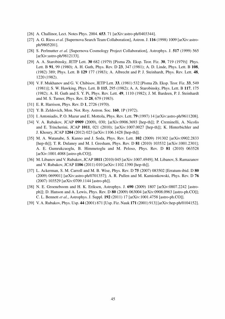
[26] A. Challinor, Lect. Notes Phys. 2004. 653. 71 [arXiv:astro-ph/0403344].[27] A. G. Riess et al. [Supernova Search Team Collaboration], Astron. J. 116 (1998) 1009 [arXiv:astro-

ph/9805201].[28] S. Perlmutter et al. [Supernova Cosmology Project Collaboration], Astrophys. J. 517 (1999) 565

[arXiv:astro-ph/9812133].[29] A. A. Starobinsky, JETP Lett. 30 682 (1979) [Pisma Zh. Eksp. Teor. Fiz. 30, 719 (1979)] Phys.

Lett. B 91, 99 (1980); A. H. Guth, Phys. Rev. D 23, 347 (1981); A. D. Linde, Phys. Lett. B 108,(1982) 389; Phys. Lett. B 129 177 (1983); A. Albrecht and P. J. Steinhardt, Phys. Rev. Lett. 48,1220 (1982).

[30] V. F. Mukhanov and G. V. Chibisov, JETP Lett. 33, (1981) 532 [Pisma Zh. Eksp. Teor. Fiz. 33, 549(1981)]; S. W. Hawking, Phys. Lett. B 115, 295 (1982); A. A. Starobinsky, Phys. Lett. B 117, 175(1982); A. H. Guth and S. Y. Pi, Phys. Rev. Lett. 49, 1110 (1982); J. M. Bardeen, P. J. Steinhardtand M. S. Turner, Phys. Rev. D 28, 679 (1983).

[31] E. R. Harrison, Phys. Rev. D 1, 2726 (1970).[32] Y. B. Zeldovich, Mon. Not. Roy. Astron. Soc. 160, 1P (1972).[33] I. Antoniadis, P. O. Mazur and E. Mottola, Phys. Rev. Lett. 79 (1997) 14 [arXiv:astro-ph/9611208].[34] V. A. Rubakov, JCAP 0909 (2009), 030; [arXiv:0906.3693 [hep-th]]; P. Creminelli, A. Nicolis

and E. Trincherini, JCAP 1011, 021 (2010); [arXiv:1007.0027 [hep-th]]; K. Hinterbichler andJ. Khoury, JCAP 1204 (2012) 023 [arXiv:1106.1428 [hep-th]].

[35] M. A. Watanabe, S. Kanno and J. Soda, Phys. Rev. Lett. 102 (2009) 191302 [arXiv:0902.2833[hep-th]]; T. R. Dulaney and M. I. Gresham, Phys. Rev. D 81 (2010) 103532 [arXiv:1001.2301];A. E. Gumrukcuoglu, B. Himmetoglu and M. Peloso, Phys. Rev. D 81 (2010) 063528[arXiv:1001.4088 [astro-ph.CO]].

[36] M. Libanov and V. Rubakov, JCAP 1011 (2010) 045 [arXiv:1007.4949]; M. Libanov, S. Ramazanovand V. Rubakov, JCAP 1106 (2011) 010 [arXiv:1102.1390 [hep-th]].

[37] L. Ackerman, S. M. Carroll and M. B. Wise, Phys. Rev. D 75 (2007) 083502 [Erratum-ibid. D 80(2009) 069901] [arXiv:astro-ph/0701357]; A. R. Pullen and M. Kamionkowski, Phys. Rev. D 76(2007) 103529 [arXiv:0709.1144 [astro-ph]].

[38] N. E. Groeneboom and H. K. Eriksen, Astrophys. J. 690 (2009) 1807 [arXiv:0807.2242 [astro-ph]]; D. Hanson and A. Lewis, Phys. Rev. D 80 (2009) 063004 [arXiv:0908.0963 [astro-ph.CO]];C. L. Bennett et al., Astrophys. J. Suppl. 192 (2011) 17 [arXiv:1001.4758 [astro-ph.CO]].

[39] V. A. Rubakov, Phys. Usp. 44 (2001) 871 [Usp. Fiz. Nauk 171 (2001) 913] [arXiv:hep-ph/0104152].

45