Introduction - Union Collegeantipasto.union.edu/~andersoa/mer331/StarCCM Tutorial.pdf · STAR-CCM+ User Guide 6922 Version 7.06 Introduction Welcome to the STAR-CCM+ introductory

STAR-CCM+ User Guide 6922

Version 7.06

Introduction

Welcome to the STAR-CCM+ introductory tutorial. In this tutorial, you explore the important concepts and workflow. Complete this tutorial before attempting any others.

Throughout this tutorial, links to other sections of the online documentation explore important concepts. For example, for a clearer understanding of the changes to typeface in the tutorials, refer to the typographic conventions.

This tutorial is useful in addition to STAR-CCM+ training. For more help, contact your local CD-adapco office. A list of contacts is found at: http://www.cd-adapco.com/about/locations.html.

The case is a transonic flow over an idealized symmetrical blunt body in a wind tunnel.

The tutorial workflow includes:• Importing the geometry files.• Generating a polyhedral mesh.• Setting boundary names and types.

STAR-CCM+ User Guide Starting a STAR-CCM+ Simulation 6923

Version 7.06

• Defining the models in the continua and applying them to the regions.• Defining the region conditions, values, and boundary conditions.• Running the simulation.• Post-processing the results.

These steps follow the general workflow for STAR-CCM+.

Starting a STAR-CCM+ SimulationIf you have not already done so, launch STAR-CCM+ using the appropriate instructions for your operating system.

After a brief display of the splash screen, the STAR-CCM+ client workspace opens without loading an existing simulation or creating a simulation. This interface to the STAR-CCM+ software is a self-contained graphical user interface (GUI) with panes and subwindows. Some of the GUI terminology is shown in the following screenshot.


Version 7.06

The menu bar provides access to application-wide actions, with some of the more important actions being duplicated in the toolbar.• Let the mouse hover over any of the buttons in the toolbar.

A short description of what that button does appears in a tooltip.

Creating a Simulation• Start a simulation by selecting File > New Simulation from the menu bar.


Version 7.06

The Create a New Simulation dialog appears.

STAR-CCM+ is a client-server application with the client (user interface or batch interpreter) running in one process, and the server (the solver) running in another process. Start a server process on the same machine as the client using the settings from the above dialog.

Ticking the Remote Server checkbox allows you to start the server process on another machine. The client and server can run on machines of different architectures. The server can also run in parallel mode.


Version 7.06

• In the Create a New Simulation dialog, click OK.

A new window containing a simulation object tree is created in the Explorer pane, with the name Star 1. The initial folder nodes for this simulation are shown in the following screenshot. Other nodes are added to the object tree as you progress further.

As the new simulation is created, a window that is named Output appears in the lower-right portion of the STAR-CCM+ workspace. The Output window describes the progress of actions in the simulation.


Version 7.06

Working with Objects

Much of your interaction with the simulation are through the objects in the simulation tree that was added to the Explorer pane.

The tree represents all the objects in the simulation. Nodes are added in later sections when a geometry is imported and models are defined in the continuum. Most of your interaction with the simulation is by selecting nodes in the tree and:• Right-clicking to expose an action menu.• Using keys to, for example, copy and delete objects.• Dragging objects to other tree nodes or onto visualization displays.

The handle next to a node indicates that subnodes exist below that one. To open a node and show the subnodes, click the handle. To close it, do the same for an open node.

STAR-CCM+ User Guide Saving and Naming a Simulation 6928

Version 7.06

Most objects in the tree have one or more properties that define the object. Access to the properties is through the table.

To modify the properties of an object, click its node once to select it. Edit most types of properties in the value cell. Otherwise, when setting values of complex properties, click the property customizer button to the right of the value. A property-specific dialog opens.

Saving and Naming a SimulationThe simulation file (.sim) contains STAR-CCM+ analysis setup, runtime, and results information. Save this new simulation to disk and give it a sensible name:• Select File > Save As.

STAR-CCM+ User Guide Importing the Geometry 6929

Version 7.06

• Navigate to the directory where you want to locate the file.

• In the Save dialog, type bluntBody.sim into the File Name text box and click Save.

The title of the simulation window in the Explorer pane updates to reflect the new name.

It is useful to save work in progress periodically. This tutorial includes reminders to save the simulation at the end of each section. If you would like to return to a stage of the tutorial at a later stage, save it with a unique name.

Importing the GeometryBefore solving this case, you can recognize that the flow is likely to be symmetrical in two planes around the body. Hence, only a quarter of the geometry is modeled. This symmetry condition reduces computational costs and solution time without losing information or accuracy.

STAR-CCM+ provides tools to generate the geometry, but for this tutorial you start from a pre-generated Parasolid file of the design.

The first step in this tutorial is to import the geometry.• Select File > Import > Import Surface Mesh from the menu bar.


Version 7.06

• In the Open dialog, navigate to the doc/startutorialsdata/introduction/data subdirectory of your STAR-CCM+ installation directory and select file bluntBody.x_t.

• To start the import, click Open.The Import Surface Options dialog appears.


Version 7.06

• Select Create new Part from the Import Mode box.

• Click OK to import the geometry.

STAR-CCM+ provides feedback on the import process in the Output window. A new geometry scene is created in the Graphics window and shows the imported geometry.• In the simulation tree, expand the Geometry > Parts node to see the new


Version 7.06

bluntBody part.

The imported geometry represents the fluid volume around the body in the wind tunnel.• Save the simulation by clicking the (Save) button.

STAR-CCM+ User Guide Visualizing the Imported Geometry 6933

Version 7.06

Visualizing the Imported GeometryThe Geometry Scene 1 display is already present in the Graphics window. Initially, solid, colored surfaces show the surfaces of the geometry.

A new geometry scene contains:• A part displayer, Geometry 1, which contains all faces in the geometry

part and is preset to display a shaded surface.• A second part displayer, Outline, which also contains all faces in the

geometry part and is preset to display the mesh outline.

Panning, Zooming and Rotating the View

In the Graphics window, all three mouse buttons have drag operations that change the view of the geometry:• To rotate about the selected point, hold down the left mouse button and

drag.• To zoom in or out, hold down the middle mouse button and drag.

STAR-CCM+ User Guide Visualizing the Imported Geometry 6934

Version 7.06

• To translate or pan, hold down the right mouse button and drag.• To rotate around an axis perpendicular to the screen, press the <Ctrl>

key and hold down the left mouse button while dragging.

There are also several “hot” keys that rotate the view:• To align with the X-Y plane, press the <T> key.• To align with the Y-Z plane, press the <F> key.• To align with the Z-X plane, press the <S> key.• To fit the view within the Graphics window, press the <R> key.• Adjust the view as shown in the following screenshot.

• Save the simulation .

STAR-CCM+ User Guide Defining Boundary Surfaces 6935

Version 7.06

Defining Boundary SurfacesThe following illustration gives an overview of how you set up this problem.

To facilitate boundary creation, identify the surfaces to become boundaries:• Open the Geometry > Parts > bluntBody > Surfaces > Faces node.• Right-click the Faces node and from the pop-up menu, select Split by

Index Description

1 Stagnation Boundary

2 Wall

3 Symmetry Planes

4 Pressure Boundary

5 Slip Walls


Version 7.06

Patch.

The Split Part Surface by Patch dialog appears.• In Geometry Scene 1, select the face in the low X direction, rotating the


Version 7.06

geometry as necessary.

• Type Inlet in the Part Surface Name field.

• Click the Create button.

The face is removed from the scene and the new surface appears within the surfaces manager node belonging to the parent part.


Version 7.06

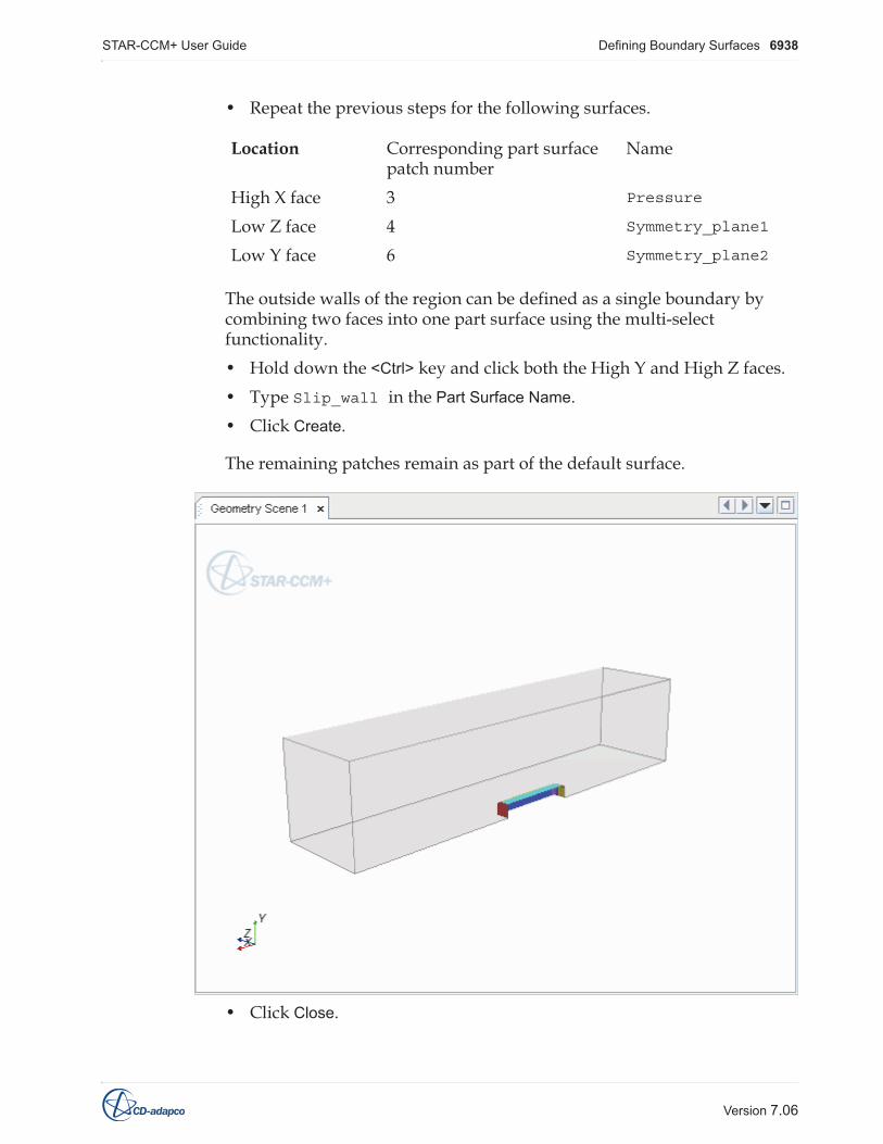
• Repeat the previous steps for the following surfaces.

The outside walls of the region can be defined as a single boundary by combining two faces into one part surface using the multi-select functionality.• Hold down the <Ctrl> key and click both the High Y and High Z faces.• Type Slip_wall in the Part Surface Name.• Click Create.

The remaining patches remain as part of the default surface.

• Click Close.

Location Corresponding part surface patch number

Name

High X face 3 Pressure

Low Z face 4 Symmetry_plane1

Low Y face 6 Symmetry_plane2


Version 7.06


Renaming the Surface and Part

Renaming nodes is a common operation in STAR-CCM+. There are two ways a node can be renamed. Rename the Faces node and the bluntBody part.• Select the Geometry > Parts > bluntBody node.• Press <F2>.• Rename the part subdomain-1

• Press <Enter> or click another node to accept.

To rename the Faces part surface, the previous method can be used. Use the alternative right-click menu option:• Right-click the Geometry > Parts > subdomain-1 > Surfaces > Faces node

STAR-CCM+ User Guide Assigning Parts to Regions 6940

Version 7.06

and select Rename...

• In the Rename dialog, enter Inner_wall and click OK.

The parts are ready to be converted to a region and boundaries.• Save the simulation .

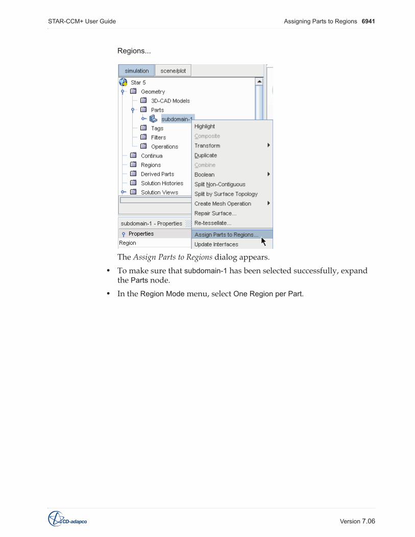
Assigning Parts to RegionsGeometry parts are used to prepare the spatial representation of the model. The computational model to which physics can be applied is defined in terms of regions, boundaries, and interfaces. Create a region and associated boundaries from the geometry part and its surfaces:• Right-click Geometry > Parts > subdomain-1 and select Assign Parts to


Version 7.06

Regions...

The Assign Parts to Regions dialog appears.• To make sure that subdomain-1 has been selected successfully, expand

the Parts node.• In the Region Mode menu, select One Region per Part.


Version 7.06

• Set the Boundary Mode to One boundary per part surface.

• Click the Create Regions button.• Close the dialog.

The portion of the object tree below the Regions node appears as shown in the following screenshot. All of the surfaces appear as individual boundaries within the region.

STAR-CCM+ User Guide Setting Boundary Types 6943

Version 7.06


Setting Boundary TypesHaving given the boundaries sensible names, you can set the boundary types. • Select the Symmetry_plane1 node and set Type to Symmetry Plane.

The boundary node icon changes to reflect the new type.• Using the same technique, change Symmetry_plane2 to Symmetry Plane.

For compressible flows, the most appropriate inflow and outflow types are stagnation inlet and pressure outlet.• Change the type of the Inlet boundary to Stagnation Inlet and the type of

the Pressure boundary to Pressure Outlet.

The Slip_wall and Inner_wall boundaries retain the default Wall type. Slip walls are boundary conditions and are set up later.• Save the simulation .

Selecting Parts• Click a part in the Geometry Scene 1 display, for example the High X face.


Version 7.06

The object becomes highlighted and a label appears with the name of the object selected.

In the bluntBody object tree, the node that corresponds to this object is also highlighted.

Conversely, if a boundary node is selected in the bluntBody tree, the surface corresponding to that boundary is highlighted in the Graphics window.

Adding and Removing Parts from a Scene

To remove and add some parts, use the part selector dialog.


Version 7.06

• Open the Scenes > Geometry Scene 1 > Displayers > Geometry 1 > Parts node and click the ellipsis (Custom Editor) for the Parts value.

The Parts dialog appears.

• Click Clear Selection.• Select Regions > subdomain-1 > Inner_wall.

• Click OK.


Version 7.06

This selection removes the solid-colored boundaries representing the wind tunnel from the scene, leaving the outlines and the blunt body.

Add those parts back to the scene using a drag-and-drop method:• Open the Regions > subdomain-1 > Boundaries node.• To extend your selection, hold down the <Ctrl> key and select all the

boundary nodes except Inner_wall.• Release the <Ctrl> key but continue to keep the left mouse button

pressed.• Drag the nodes onto the display and release the left mouse button.

A pop-up menu appears.

Use this menu to choose which of the part displayers in the scene receive the parts that you have dragged across.

STAR-CCM+ User Guide Generating the Mesh 6947

Version 7.06

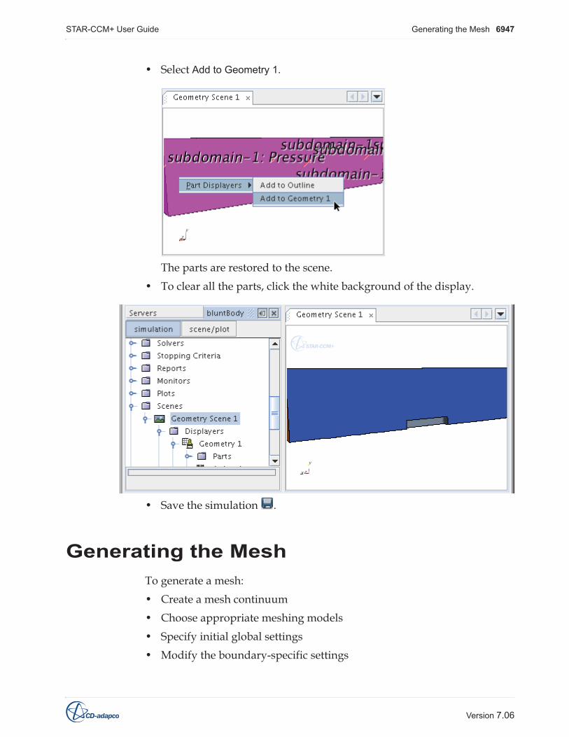
• Select Add to Geometry 1.

The parts are restored to the scene. • To clear all the parts, click the white background of the display.


Generating the MeshTo generate a mesh:• Create a mesh continuum• Choose appropriate meshing models• Specify initial global settings • Modify the boundary-specific settings


Version 7.06

Creating the Mesh Continuum

The mesh continuum is used to specify the required meshing models.• Right-click Continua.• Select New > Mesh Continuum.

A new node, Mesh 1, is added to the simulation tree.

Choosing Meshing Models

The meshing continuum has a Models node which you can now populate.


Version 7.06

• Right-click the Mesh 1 node and choose Select Meshing Models...

In the Mesh 1 Model Selection dialog:• Select Surface Remesher from the Surface Mesh group box.• Select Polyhedral Mesher and Prism Layer Mesher from the Volume Mesh

group box.

The enabled models section appears as shown in the following screenshot.

• Click Close.• Expand the Models and Reference Values managers.


Version 7.06

The simulation tree appears as shown in the following screenshot.

Specifying the Mesh Settings

Generating a mesh often requires several iterations to achieve the desired density and distribution of cells. In this tutorial, you generate a volume mesh, add some simple refinement, and regenerate. • Select the Continua > Mesh 1 > Reference Values > Base Size node and set

Value to 0.01 mWith this base size, approximately 8 cells are created across the width of the region.

• Select Continua > Mesh 1 > Reference Values > Number of Prism Layers and


Version 7.06

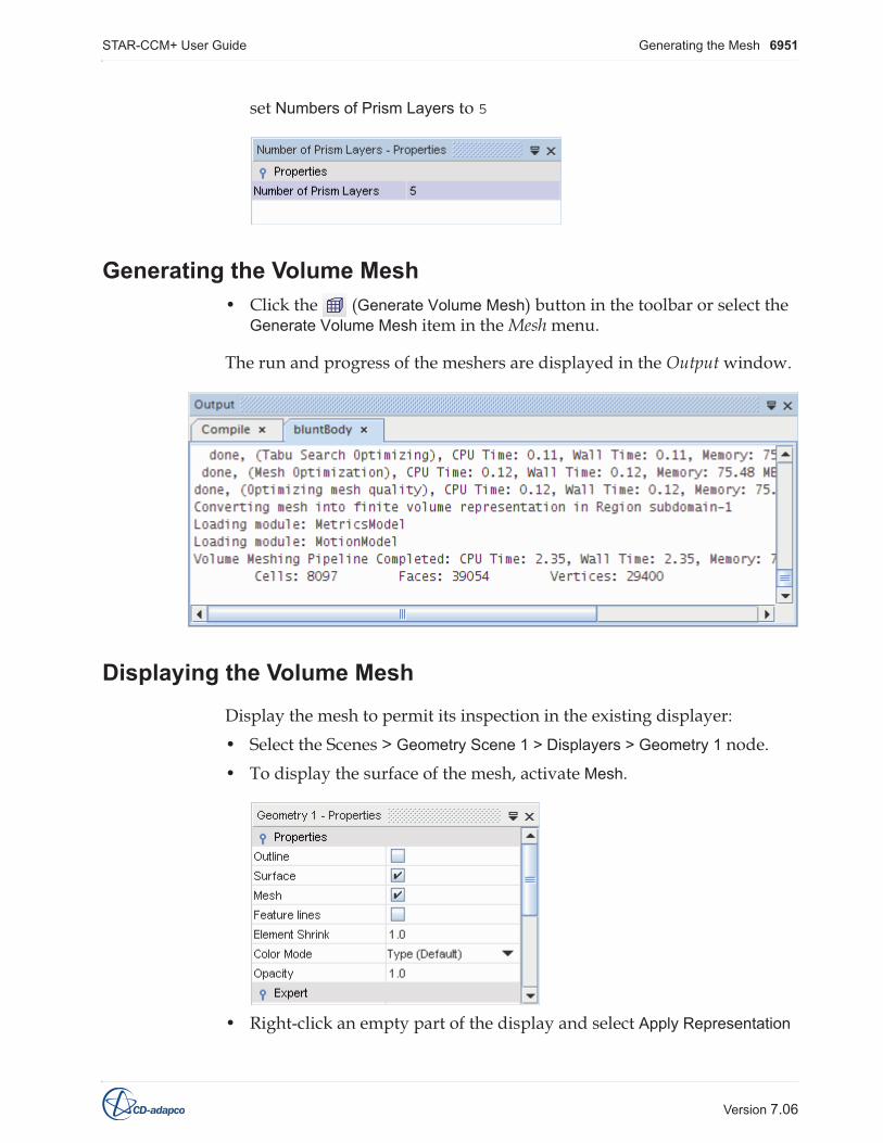
set Numbers of Prism Layers to 5

Generating the Volume Mesh• Click the (Generate Volume Mesh) button in the toolbar or select the

Generate Volume Mesh item in the Mesh menu.

The run and progress of the meshers are displayed in the Output window.

Displaying the Volume Mesh

Display the mesh to permit its inspection in the existing displayer: • Select the Scenes > Geometry Scene 1 > Displayers > Geometry 1 node.• To display the surface of the mesh, activate Mesh.

• Right-click an empty part of the display and select Apply Representation


Version 7.06

> Volume Mesh.


Version 7.06

This action reveals the mesh on the boundaries.


Refining the Mesh

The prism layer has been generated on the inner and the slip walls by default. Because a fluid boundary layer does not form on slip walls, you can customize the prism mesh settings on that boundary. • Select the Regions > subdomain-1 > Boundaries > Slip_wall > Mesh

Conditions node and set Customize Prism Mesh to Disable.


Version 7.06

To provide better definition of the blunt body, modify the surface mesh at the inner wall:• Select the Regions > subdomain-1 > Boundaries > Inner_wall > Mesh

Conditions > Custom Surface Size node and activate Custom Surface Size.

A new Mesh Values manager appears.• Select the Surface Size node and set Relative/Absolute to Absolute.

• Select the Surface Size > Absolute Minimum Size node and make sure that Value is 0.0010 m

To regenerate the mesh:• Click the (Generate Volume Mesh) button.• Zoom in to the area around the slip walls and inner walls to see the

STAR-CCM+ User Guide Setting Up the Physics Models 6955

Version 7.06

improved mesh.

This mesh is satisfactory for an initial solution.• Save the simulation .

Setting Up the Physics ModelsPhysics models define the primary variables of the simulation, including pressure, temperature and velocity, and the mathematical formulation. In this example, the flow is turbulent and compressible. You use the Coupled Flow model together with the default K-Epsilon Turbulence model.

In STAR-CCM+, the physics models are defined on a physics continuum.

Selecting Models

To access the physics continuum: • Right-click Continua and select New > Physics Continuum.


Version 7.06

• Open the Continua node, which contains the default Physics 1 node.

• Right-click the Physics 1 node and choose Select models...

The Physics Model Selection dialog appears as shown in the following


Version 7.06

screenshot.

• Select the Gas radio button from the Material group box, since this exercise involves an idealized gas (air).

Since the Auto-select recommended models checkbox is activated, the Physics Model Selection dialog guides you through the model selection process by selecting certain default models automatically as you make some choices.

Certain models, when activated in a continuum, require other models also to be activated in that continuum. For instance, once a continuum contains a liquid or a gas, it also needs a flow model. Once it has a flow model, it needs a viscous model (inviscid, laminar, or turbulent). Once turbulence is activated within a fluid continuum, select a turbulence model. The prompt


Version 7.06

Additional model selections are required alerts you to the fact that you have not completed the model selection.

The following selections are required for this simulation:• Select Coupled Flow from the Flow group box.• Select Ideal Gas from the Equation of State group box.

The Coupled Energy model is selected automatically.• Select Steady from the Time group box.• Select Turbulent from the Viscous Regime group box.• Select K-Epsilon Turbulence from the Reynolds-Averaged Turbulence group

box.The Realizable K-Epsilon Two-Layer and the Two-Layer All y+ Wall Treatment models are selected automatically.

To reverse part or all of the model selection process, simply clear the checkboxes of the models you wish to deactivate. Other active models require the selections that are grayed out. Therefore, deactivate the models that are not grayed out to begin with.


Version 7.06

When complete, the Physics Model Selection dialog appears as shown in the following screenshot:

No optional models are required for this simulation.• Click Close.• To see the selected models in the simulation tree, open the Continua

node in the bluntBody window of the Explorer pane.

The color of the Physics 1 node has turned from gray to blue to indicate that models have been selected. • To display the selected models, open the Physics 1 node and then the


Version 7.06

Models node.

Setting Model Properties

After defining the continua models, the model properties can be reviewed in the object tree.

STAR-CCM+ User Guide Setting Initial Conditions 6961

Version 7.06

When you select the Gas model, the properties of air such as dynamic viscosity are used by default. Since this problem uses air, the properties are acceptable.• Save the simulation .

Setting Initial ConditionsInitial conditions in a continuum specify the initial field data for the simulation. Examples of initial conditions are:• Pressure• Temperature• Velocity components• Turbulence quantities

Each model requires sufficient information so that the primary variables of the model can be set. For some models, such as turbulence models, the option of specifying the information in a more convenient form is presented. For example, turbulence intensity and turbulent viscosity ratio instead of turbulent kinetic energy and turbulent dissipation rate.

In steady-state simulations, the solution ought to converge independently of the initial field. However, the initial field still affects the path to convergence, and with it the cost in computing power. Therefore specify initial conditions and values judiciously, particularly when the physics is complex.

Specifying the Initial Conditions for the Case

The stagnation inlet boundary has conditions that correspond to a Mach number of 0.75. The equivalent freestream velocity is roughly 300 m/s, the value you use to initialize the velocity field.• Open the Continua > Physics 1 > Initial Conditions node.• Open the Velocity > Constant node and set Value to 300,0,0

STAR-CCM+ User Guide Defining the Region Continuum 6962

Version 7.06

STAR-CCM+ adds the decimal point and units automatically, so by simply typing 300,0,0 you get an entry of [300.0, 0.0, 0.0] m/s.• In the same Initial Conditions node, open the Turbulent Viscosity Ratio node

and select the Constant node.• Set Value to 50, which is the same as the turbulent viscosity ratio that is

set on the stagnation boundary condition.


Defining the Region ContinuumAssociate each region with a continuum. On the other hand, you can associate a continuum with zero, one or more regions. Multiple continua can be defined and each region assigned a different one. In this tutorial, only one geometry part is present, which requires a single region to represent it, which was named subdomain-1. There is a simple way to determine which set of continua models are allocated to a region.• Select the subdomain-1 node in the Regions node.

• Set the Physics Continuum property to Physics 1, the name of the continuum where you defined all the models earlier.

During this tutorial, there is one continuum in the above drop-down list, but as you add more (to the Continua node in the simulation tree), they are

STAR-CCM+ User Guide Setting Boundary Conditions and Values 6963

Version 7.06

added to the drop-down list. This process determines which continua is used in the analysis, though continua can be defined and left unused.

Setting Boundary Conditions and ValuesAlthough the concept of a boundary type is fairly unambiguous (wall, stagnation inlet, and so on.), models need more information to deal with the type. Conditions provide this information. For example, with a boundary of type wall, the conditions specify whether this wall is to be a no-slip wall, a slip wall, or a moving wall. The conditions also tell you whether you want to apply a specified temperature (Dirichlet) thermal boundary condition or a specified heat flux (Neumann) thermal boundary condition.

The types and conditions inform models how to deal with a boundary (or region or interface) but they do not specify actual numerical input. Values provide this input. Value nodes are added in response to choices made on conditions nodes.

Setting Inlet Conditions and Values

To achieve a Mach number of approximately 0.75 at the inlet, isentropic relations were used to determine the inlet total pressure and outlet static pressure for a given total temperature. For an outlet static pressure equal to one atmosphere (absolute) and a static temperature of 300 K, the inlet total pressure is 164,904 Pa (absolute). The inlet total temperature is 344.8 K.

The boundary values are specified as gauge pressures. Therefore, using the default reference pressure of 101,325 Pa (one atmosphere), set the inlet total pressure to 63,579 Pa (gauge). The outlet static pressure is 0 Pa (gauge), the default value.• Open the Regions > subdomain-1 > Boundaries node.• Open the Inlet, Physics Values and Total Pressure nodes, and select the


Version 7.06

Constant node.

• Set Value to 63579

The total pressure setting is relative to the operating pressure value of 101,325 Pa. A supersonic static pressure is also required as part of a stagnation inlet condition but is only used if the inlet velocity becomes supersonic at some instance during solution iteration. The default value of 0.0 Pa relative pressure is sufficient as long as supersonic flow does not occur.

The next value to set is the total temperature.• In the same Physics Values node, open the Total Temperature node and

select the Constant node.


Version 7.06

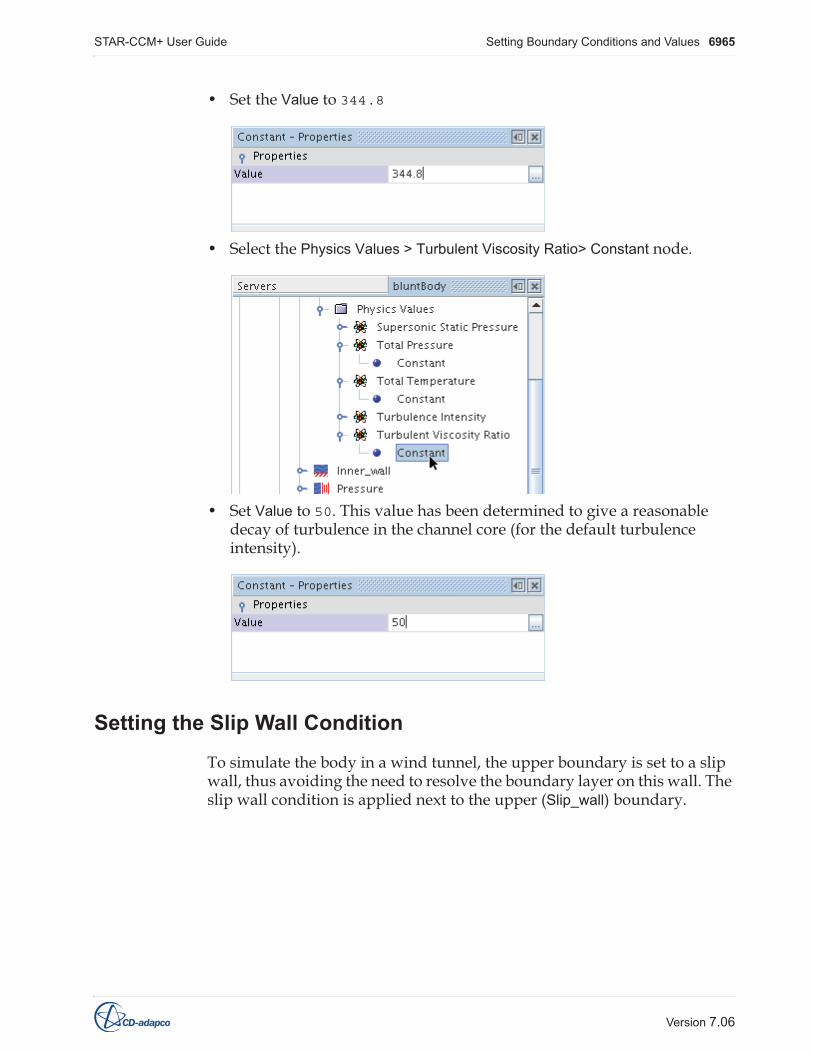
• Set the Value to 344.8

• Select the Physics Values > Turbulent Viscosity Ratio> Constant node.

• Set Value to 50. This value has been determined to give a reasonable decay of turbulence in the channel core (for the default turbulence intensity).

Setting the Slip Wall Condition

To simulate the body in a wind tunnel, the upper boundary is set to a slip wall, thus avoiding the need to resolve the boundary layer on this wall. The slip wall condition is applied next to the upper (Slip_wall) boundary.

STAR-CCM+ User Guide Setting Solver Parameters and Stopping Criteria 6966

Version 7.06

• Select the Slip_wall > Physics Conditions > Shear Stress Specification node.

• Set Method to Slip.


Setting Solver Parameters and Stopping Criteria

Use the default Courant number of 5 for this part of the calculation. To set a stopping criterion:• Select the Stopping Criteria > Maximum Steps node.

• Set the Maximum Steps to 300

STAR-CCM+ User Guide Visualizing the Solution 6967

Version 7.06

The solution does not converge in this number of iterations. The solution does not run for more than 300 iterations, unless this stopping criterion is changed or deactivated.• Save the simulation .

Visualizing the SolutionTo watch the Mach number on the blunt body and vertical symmetry plane solution developing, set up a scalar scene.• Right-click the Scenes node and select the New Scene > Scalar.

A new Scalar Scene 1 display appears.

Hide all parts except the blunt body itself and the vertical symmetry plane.• Select the new Scenes > Scalar Scene 1 > Displayers > Scalar 1 > Parts


Version 7.06

node.

• Click the (Custom Editor) in the right half of the Parts property.• In the Parts dialog, expand Regions > subdomain-1, select Inner_wall and

Symmetry_plane1, and click OK.

Define Mach number as the scalar to display:• Right-click the scalar bar (near the bottom of the Graphics window).


Version 7.06

• Select Mach Number > Lab Reference Frame from the pop-up menu.

Since the geometry of this example is symmetric, the mesh was cut into quarters with two symmetry planes to reduce computing costs. However, the symmetric repeat transform lets you create the visual effect of the complete geometry by setting up the mirror image of the model in the Graphics window. In this case, you only do one repeat so that half the model is shown.• Select the Scalar 1 node.


Version 7.06

• Set the Transform expert property to Symmetry_plane2 1.

To remove the outline:• Select the Displayers > Outline 1 node.• Clear the checkbox of the Outline property.

STAR-CCM+ User Guide Monitoring Simulation Progress 6971

Version 7.06

The scalar scene, appears as below.


Monitoring Simulation ProgressSTAR-CCM+ can dynamically monitor a quantity of interest while the solution develops. The process involves:• Setting up a report that defines the quantity of interest and the region

parts that are monitored• Defining a monitor using that report, which controls the update

frequency and normalization characteristics• Setting up an X-Y plot using that monitor

For this case, force is monitored on the body in the x-direction of the flow, which effectively is the total drag force. This process starts with the report definition.


Version 7.06

Setting Up a Report• Right-click the Reports node and select New Report > Force Coefficient.

This action creates a Force Coefficient 1 node under the Reports node.

Select the Force Coefficient 1 node and enter the settings for the report in the Properties window.

• Enter 1.277 for Reference Density, the density of the freestream air.• Enter 264.6 for Reference Velocity, the velocity at the inlet.• Enter a value of 0.0161269 for Reference Area, the projected area of the

quarter of the blunt body that is used in the simulation.• Make sure that Direction is [1.0,0.0,0.0] (for drag).


Version 7.06

Use the drag-and-drop method to select the monitored part, namely the Inner_wall boundary:• Open the Regions > subdomain-1 > Boundaries node and then drag the

Inner_wall node onto the Force Coefficient 1 node.

The Inner_wall entry is now listed in the Parts property of the Force Coefficient 1 node.

The setup for the report is now complete, and a monitor and a plot can be made from that report.

Setting Up a Monitor and a Plot• Right-click the Force Coefficient 1 node and select Create Monitor and Plot


Version 7.06

from Report.

This action creates a Force Coefficient 1 Monitor node under the Monitors node.

The existing monitors in this branch of the simulation tree are the residual monitors from the solvers that the models use. With the new monitor node selected, the default settings for the Force Coefficient 1 monitor are seen.

These settings update the plot every iteration while the solution is running.


Version 7.06

In addition to the new monitor node, a Force Coefficient 1 Monitor Plot node is created in the Plots node.

• Select the new Force Coefficient 1 Monitor Plot node.

The property settings for the plot appear.

Additional properties of the plot can be adjusted using the subnodes of the Force Coefficient 1 Plot node.

To view the plot display, either• Double-click the Force Coefficient 1 Monitor Plot node.

Or • Right-click the Force Coefficient 1 Monitor Plot node and select Open from

the pop-up menu.

STAR-CCM+ User Guide Running the Simulation 6976

Version 7.06

A Force Coefficient 1 Monitor Plot appears in the Graphics window.

This plot display is automatically updated with the drag force coefficient when the solver starts to run.

The pre-processing setup is completed. The simulation can now be run to convergence.• Save the simulation .

Running the SimulationTo run the simulation, either: • Click the (Run) button in the Solution toolbar

Or• Use the Solution > Run menu item.

The Residuals display is created automatically and shows the progress of the solver. If necessary, click the Residuals tab to bring the Residuals plot into view. An example of a residual plot is shown in a separate part of the User Guide. This example looks different from your residuals, since the plot depends on the models selected.

STAR-CCM+ User Guide Adjusting Solver Parameters and Continuing 6977

Version 7.06

The tabs at the top of the Graphics window allow you to select any one of the active displays for viewing.• To see the results, click the tab of the Scalar Scene 1 display.• Rotate and zoom if desired for a better view.

During the run, it is possible to stop the process by clicking the (Stop) button in the toolbar. If you do halt the simulation, you can resume it by clicking the (Run) button. If left alone, the simulation continues until the stopping criterion of 300 iterations is satisfied.• After the run is finished, save the simulation.

Adjusting Solver Parameters and Continuing

The default Courant number of 5 is conservative for this type of problem on a mesh of reasonable quality, so it can be increased to accelerate convergence.

Once the solution has reached the stopping criterion of 300 iterations:


Version 7.06

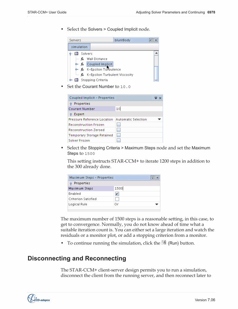
• Select the Solvers > Coupled Implicit node.

• Set the Courant Number to 10.0

• Select the Stopping Criteria > Maximum Steps node and set the Maximum Steps to 1500This setting instructs STAR-CCM+ to iterate 1200 steps in addition to the 300 already done.

The maximum number of 1500 steps is a reasonable setting, in this case, to get to convergence. Normally, you do not know ahead of time what a suitable iteration count is. You can either set a large iteration and watch the residuals or a monitor plot, or add a stopping criterion from a monitor.• To continue running the simulation, click the (Run) button.

Disconnecting and Reconnecting

The STAR-CCM+ client-server design permits you to run a simulation, disconnect the client from the running server, and then reconnect later to


Version 7.06

check on results. You can also reconnect from a different machine, even a machine of another architecture.

To disconnect the client from the server:• Open the Servers window (if it is not already open) by selecting Window

> Servers.• To see your simulation, look in the Servers window of the Explorer pane.• Reselect the simulation window in the Explorer pane, and select the File

> Disconnect menu item.

• In the OK to disconnect dialog, click OK.


Version 7.06

The client disconnects from the server, but both are still running, although the simulation window no longer appears in the client. If desired, the client can be shut down using File > Exit.

The Servers window of the Explorer pane lists all server processes (simulations) that are running locally.

Selecting the node in the tree displays the server process properties.

If the Clients property is empty (as shown above), then that server process does not have a client that is connected to it and it is possible to connect.• Connect by right-clicking the server process node in the Servers tree and

selecting Connect from the pop-up menu.

When you reconnect, none of the previously created scenes and plots are displayed in the Graphics window.

To display a scene of interest:• Double-click its node in the simulation object tree,

Or • Right-click the node and select Open.

STAR-CCM+ User Guide Visualizing Results 6981

Version 7.06

Completing the Run

At the end of the calculation, the Residuals display show most of the residuals flattening out, which is a good indicator of convergence.

To confirm that the solution has converged:• Select the Force Coefficient 1 Monitor Plot display to verify that the drag

coefficient has also flattened out.

• Once the run is finished, save the simulation.

Visualizing ResultsOnce the solution is finished, you can examine the results in scalar and vector scenes.

Examining Scalars• Make the Scalar Scene 1 display active to see the Mach number results


Version 7.06

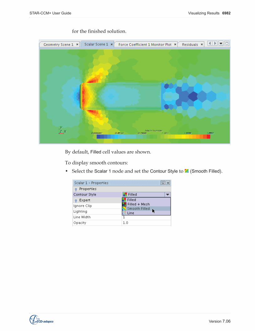
for the finished solution.

By default, Filled cell values are shown.

To display smooth contours:• Select the Scalar 1 node and set the Contour Style to (Smooth Filled).


Version 7.06

The contours of the scalar display now appear smooth.

Display two scalar values at the same time: one on the symmetry plane, the other on the inner wall:• Add another scalar displayer by right-clicking the Displayers node and

selecting New Displayer > Scalar.

The creation of the second displayer has added a second scalar bar in the display.

To view both scalar bars easily:• Point the mouse in the interior of a scalar bar to drag either one of them


Version 7.06

to a different location.

• In the display, right-click the scalar bar (blue) of the new displayer and select Pressure.

• Right-click the inner wall in the display, select Displayers, and open its submenu.

• Among the checkboxes to the right of in, clear the checkbox under Scalar1 and tick the one under Scalar 2.


Version 7.06

This single step transfers the part from one displayer to another.• Select the Scenes > Scalar Scene 1 > Displayers > Scalar 2 node.

• Set the Contour Style to (Smooth Filled).• Set the Transform expert property to Symmetry_plane2 1.

The blunt body shows pressure values while the symmetry plane shows Mach number.



Version 7.06

Examining Vectors

This section demonstrates how to examine velocity vectors in the model. In this example, you set up vectors in a reflected symmetry plane around a solid-colored blunt body.• First, create a scene by right-clicking the Scenes node.• Select New Scene > Vector.

A new Vector Scene 1 display appears.

You do not need the outlines that the Outline part displayer provides by default, so reuse that displayer to show the blunt body as a solid object.• Select the Vector Scene 1 > Displayers > Outline 1 > Parts node and click

the (Custom Editor) button. • In the Parts dialog, expand the Regions and subdomain-1 nodes.• Click Clear Selection.• Select the Inner_wall node.


Version 7.06

• Click OK.

• Select the Outline 1 node in the Displayers node.

Make the following changes to the Outline displayer properties:• Deactivate the Outline property.• Activate the Surface property.


Version 7.06

• Set the Transform expert property to Symmetry_plane2 1.

• Select the Vector 1 > Parts node and click the ellipsis (Custom Editor) for the Parts value.

• In the Parts dialog, expand the Regions and subdomain-1 nodes. Select


Version 7.06

the Symmetry_plane1 node and click OK.

• Select the Vector 1 node.

• Set the Transform expert property to Symmetry_plane2 1


Version 7.06

These settings show a solid blunt body with velocity vectors surrounding it.

It is possible to make the arrows shorter to see the vectors more clearly. • Select the Vector 1 > Glyph > Relative Length node and change Glyph

Length (%) to 2.0.

STAR-CCM+ User Guide Plotting Data on a Slice 6991

Version 7.06

The arrows now appear shorter.


Plotting Data on a SliceIn this section, you create an x-y plot to visualize the pressure coefficient (on the y-axis) along a slice of the blunt body. Create a derived part for the slice, and then create a plot using that derived part.

Creating a Derived Part

The new derived part that is created is the curve along the surface of the blunt body. It is shown in pink below.


Version 7.06

• Right-click the Scenes node and select New Scene > Geometry.

• Right-click the Derived Parts node and select New Part > Section > Plane...

A new interactive in-place dialog is activated to allow definition of the derived part.

To define the source part for this derived part:• In the Input Parts group box, click the [subdomain-1] button.• In the dialog that appears, expand the Regions and subdomain-1 nodes.• Click Clear selection.


Version 7.06

• Select the Inner_wall boundary and click OK.

The plane tool in the scene display allows interactive definition of the plane that cuts the blunt body.• Rotate and pan the image as needed so that the inner wall is in front of

the plane tool rectangle as shown.

• In the dialog, leave the Display box at its default setting.

The “barbell” represents the normal of the cutting plane, which can be changed by dragging one of the balls to another location.• The plane can also be dragged to change the origin of the cutting plane.

A bounding box slightly larger than the regions in the scene is displayed to limit the movement of the plane.


Version 7.06

• Move the mouse over the plane tool, then click-and-drag the rectangle so that it cuts the blunt body close to the symmetry plane.


Version 7.06

• Click Create and then Close.

In the bluntBody window, a node, plane section, has been added within the Derived Parts.

It is now possible to plot data on the new surface.• Save the simulation .

Plotting Simulation Data

To set up a plot of pressure coefficients for the new derived part:• In the bluntBody window, right-click the Plots node and select New Plot >

X-Y.

An empty plot node is added to the tree and opens in the Graphics window.

To select the part on which to plot:• Select the Plots > XY Plot 1 node and click the (Custom Editor) button

for the Parts property.• In the XY Plot 1 dialog, make sure that Derived parts > plane section is

ticked.• Click OK.

To set the variable to plot on the y-axis:• Select the XY Plot 1 > Y Types > Y Type 1 node and make sure that the

Type property is set to Scalar.


Version 7.06

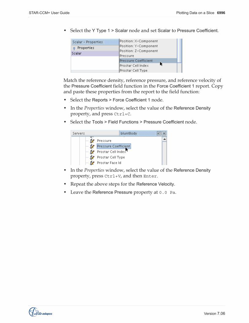
• Select the Y Type 1 > Scalar node and set Scalar to Pressure Coefficient.

Match the reference density, reference pressure, and reference velocity of the Pressure Coefficient field function in the Force Coefficient 1 report. Copy and paste these properties from the report to the field function:• Select the Reports > Force Coefficient 1 node.• In the Properties window, select the value of the Reference Density

property, and press Ctrl+C.• Select the Tools > Field Functions > Pressure Coefficient node.

• In the Properties window, select the value of the Reference Density property, press Ctrl+V, and then Enter.

• Repeat the above steps for the Reference Velocity.• Leave the Reference Pressure property at 0.0 Pa.

STAR-CCM+ User Guide Adding Streamlines 6997

Version 7.06

The plot appears as shown below.


Adding StreamlinesTo visualize streamlines in STAR-CCM+:• Create a scene • Create a streamline derived part• Add a streamline displayer, with suitable properties, to the new scene

based on the streamline derived part.

In this example, the streamline derived part is set up so that it shows the recirculating flow behind the blunt body. The part is then modified to show streamlines over the blunt body.

To create the scene:• Right-click the Scenes node.


Version 7.06

• Select New Scene > Geometry.

To create the streamline derived part:• Right-click the Derived Parts node.• Select New Part > Streamline in the bluntBody window.


Version 7.06

As with the plane section earlier, an interactive in-place dialog appears.

The entire fluid region is used as the input part for the streamline part.• Click the Input Parts button.• In the Select Objects dialog, make sure that subdomain-1 is the only part

in the Selected list.• Click Close in the Select Objects dialog.• In the Vector Field box, make sure that Velocity is selected in the

drop-down list.


Version 7.06

• For the seed mode, select Point Seed.

To position the seed point just after the back of the blunt body (in the direction of flow):• Enter the following coordinates under Seed Position: 0.05 for X, 0.01

for Y and 0.01 for Z.• Enter 0.002 for Seed Radius and 10 for Number of Points.

• Leave other settings at their defaults.• To generate the streamlines, click Create.


Version 7.06

After a few seconds, the streamlines are shown in the display.

In the bluntBody window, a streamline node appears in the Derived Parts node.

• Click Close in the interactive in-place dialog.

A new streamline displayer has been added to the scene.• Select the Displayers > Streamline Stream 1 node to modify the displayer

to customize how the streamlines appear:• Set the Mode to Tubes so that the streamlines are displayed as tubes

instead of lines.• Make sure that Orientation is set to Normals.


Version 7.06

• Specify Width at 2.0E-4, the width of the tube in meters.

• In the display, right-click the color bar and select Velocity: Magnitude.

Improve the contrast between boundaries and streamlines:• Select the Geometry 1 node and set the Color Mode to Constant.

You now fine-tune the streamline derived part.• Select the Derived Parts > streamline node and make sure that the Rotation

Scale expert property is 1.0• Select the streamline > 2nd Order Integrator node and set the Integration

Direction to Both so that the streamlines are generated both upstream and downstream.


Version 7.06

In the Expert properties:• Set Initial Integration Step to 0.1 to provide more resolution to the

streamlines.• Set Maximum Propagation to 5.0• Set Max Steps to 1000

This option, together with the maximum propagation, provide a stopping criterion to make sure that the streamlines are not calculated endlessly.

The modified streamlines appear as below.

The next step involves moving the seed point of the streamline derived part to the front of the blunt body.• Select the 2nd Order Integrator node and change Integration Direction to

Forward. • Select the streamline > Point Seed node and set the x-value of the Center

to -0.05, so that the value of the property is -0.05, 0.01, 0.01

STAR-CCM+ User Guide Closing and Reopening the Simulation 7004

Version 7.06

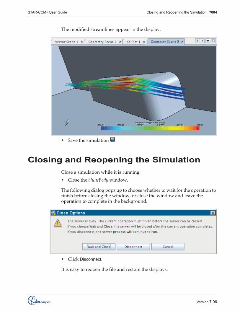
The modified streamlines appear in the display.


Closing and Reopening the SimulationClose a simulation while it is running:• Close the bluntBody window.

The following dialog pops up to choose whether to wait for the operation to finish before closing the window, or close the window and leave the operation to complete in the background.

• Click Disconnect.

It is easy to reopen the file and restore the displays.

STAR-CCM+ User Guide Summary 7005

Version 7.06

• Select File > Recent Files > /bluntBody.sim.

SummaryThis tutorial of STAR-CCM+ introduced the following steps:• Starting the code and creating a simulation.• Saving and naming the simulation.• Importing a geometry file.• Visualizing the imported geometry.• Splitting and naming the geometry surfaces.• Renaming techniques.• Changing types of boundaries.• Designing a three-dimensional mesh• Visualizing the mesh.• Selecting the physics models.• Defining the initial conditions.• Defining the boundary conditions and values.• Setting the solver parameters and stopping criteria.• Setting up a monitoring report and plot.• Running the solver until the residuals are satisfactory.• Disconnecting from a server and reconnecting during a run.• Analyzing results using the visualization, monitor-plot, and XY-plot

features.• Creating streamlines.• Reopening a simulation.

Documents

Introduction - Union Collegeantipasto.union.edu/~andersoa/mer331/StarCCM Tutorial.pdf · STAR-CCM+ User Guide 6922 Version 7.06 Introduction Welcome to the STAR-CCM+ introductory