VERSION 4.4

Introduction toPipe Flow Module

C o n t a c t I n f o r m a t i o nVisit the Contact COMSOL page at www.comsol.com/contact to submit general inquiries, contact

Technical Support, or search for an address and phone number. You can also visit the Worldwide

Sales Offices page at www.comsol.com/contact/offices for address and contact information.

If you need to contact Support, an online request form is located at the COMSOL Access page at

www.comsol.com/support/case.

Other useful links include:

• Support Center: www.comsol.com/support

• Product Download: www.comsol.com/support/download

• Product Updates: www.comsol.com/support/updates

• COMSOL Community: www.comsol.com/community

• Events: www.comsol.com/events

• COMSOL Video Center: www.comsol.com/video

• Support Knowledge Base: www.comsol.com/support/knowledgebase

Part number. CM022801

I n t r o d u c t i o n t o t h e P i p e F l o w M o d u l e © 1998–2013 COMSOL

Protected by U.S. Patents 7,519,518; 7,596,474; 7,623,991; and 8,457,932. Patents pending.

This Documentation and the Programs described herein are furnished under the COMSOL Software License Agreement (www.comsol.com/sla) and may be used or copied only under the terms of the license agreement.

COMSOL, COMSOL Multiphysics, Capture the Concept, COMSOL Desktop, and LiveLink are either registered trademarks or trademarks of COMSOL AB. All other trademarks are the property of their respective owners, and COMSOL AB and its subsidiaries and products are not affiliated with, endorsed by, sponsored by, or supported by those trademark owners. For a list of such trademark owners, see www.comsol.com/tm.

Version: November 2013 COMSOL 4.4

Contents

Introduction . . . . . . . . . . . . . . . . . . . . . . . . . . . . . . . . . . . . . . . . . . . 1

The Applications . . . . . . . . . . . . . . . . . . . . . . . . . . . . . . . . . . . . . . . . . . 2

The Pipe Flow Module Interfaces . . . . . . . . . . . . . . . . . . . . . . . . . 6

The Physics Interfaces by Space Dimension and Study Type . . . . . 7

The Model Libraries Window . . . . . . . . . . . . . . . . . . . . . . . . . . . . 9

Tutorial Example: Geothermal Heating from a Pond Loop . . . 10

| i

ii |

Introduction

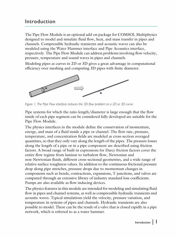
The Pipe Flow Module is an optional add-on package for COMSOL Multiphysics designed to model and simulate fluid flow, heat, and mass transfer in pipes and channels. Compressible hydraulic transients and acoustic waves can also be modeled using the Water Hammer interface and Pipe Acoustics interface, respectively. The Pipe Flow Module can address problems involving flow velocity, pressure, temperature and sound waves in pipes and channels.Modeling pipes as curves in 2D or 3D gives a great advantage in computational efficiency over meshing and computing 3D pipes with finite diameter.

Figure 1: The Pipe Flow interface reduces the 3D flow problem to a 2D or 3D curve

Pipe systems for which the ratio length/diameter is large enough that the flow inside of each pipe segment can be considered fully developed are suitable for the Pipe Flow Module.The physics interfaces in the module define the conservation of momentum, energy, and mass of a fluid inside a pipe or channel. The flow rate, pressure, temperature, and concentration fields are modeled as cross-section averaged quantities, so that they only vary along the length of the pipes. The pressure losses along the length of a pipe or in a pipe component are described using friction factors. A broad range of built-in expressions for Darcy friction factors cover the entire flow regime from laminar to turbulent flow, Newtonian and non-Newtonian fluids, different cross-sectional geometries, and a wide range of relative surface roughness values. In addition to the continuous frictional pressure drop along pipe stretches, pressure drops due to momentum changes in components such as bends, contractions, expansions, T-junctions, and valves are computed through an extensive library of industry standard loss coefficients. Pumps are also available as flow inducing devices.The physics features in this module are intended for modeling and simulating fluid flow in pipes and channel systems, as well as compressible hydraulic transients and acoustic waves. Typical simulations yield the velocity, pressure variation, and temperature in systems of pipes and channels. Hydraulic transients are also possible to model. These can be the result of a valve that is closed rapidly in a pipe network, which is referred to as a water hammer.

Introduction | 1

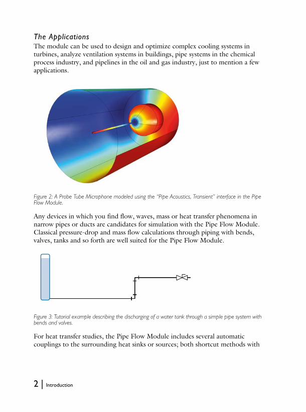
The ApplicationsThe module can be used to design and optimize complex cooling systems in turbines, analyze ventilation systems in buildings, pipe systems in the chemical process industry, and pipelines in the oil and gas industry, just to mention a few applications.

Figure 2: A Probe Tube Microphone modeled using the “Pipe Acoustics, Transient” interface in the Pipe Flow Module.

Any devices in which you find flow, waves, mass or heat transfer phenomena in narrow pipes or ducts are candidates for simulation with the Pipe Flow Module. Classical pressure-drop and mass flow calculations through piping with bends, valves, tanks and so forth are well suited for the Pipe Flow Module.

Figure 3: Tutorial example describing the discharging of a water tank through a simple pipe system with bends and valves.

For heat transfer studies, the Pipe Flow Module includes several automatic couplings to the surrounding heat sinks or sources; both shortcut methods with

2 | Introduction

semi-empirical correlations for forced and natural convection, and also direct coupling to a 3D solid, in which the pipe is embedded.

Figure 4: Methods for heat transfer to the surroundings, from left to right: forced convection, natural convection, solid conduction.

An example of an application which demonstrates the capabilities of pipe-solid coupling is the Mold Cooling model in the Pipe Flow model library. When manufacturing devices in polymeric materials, the structural integrity of the end product is very sensitive to the cooling history in the mold.

Figure 5: The heat transfer to the cooling channels embedded in a cooling mold is simulated to understand the controlled cooling of a polyurethane steering wheel. The Nonisothermal Pipe Flow interface is used in the model.

With the capabilities of modeling the transfer of chemical compounds diluted in fluids flowing through thin pipes, the pipe flow module allows for complex

Introduction | 3

chemical reaction modeling. This can include mass transfer, chemical kinetics, heat transfer, and pressure drop calculations in the same model.

Figure 6: Temperature distribution in an autothermal chemical reactor. The model includes mass transport, chemical kinetics, heat transfer, and pressure drop and flow calculations.

Thanks to COMSOL’s strong capabilities in handling so-called nonlinear materials, such as non-Newtonian fluids and materials with highly temperature dependent physical properties, oil and gas applications can be readily modeled. One example is crude oil pipelines, where the viscous heating effects combined

4 | Introduction

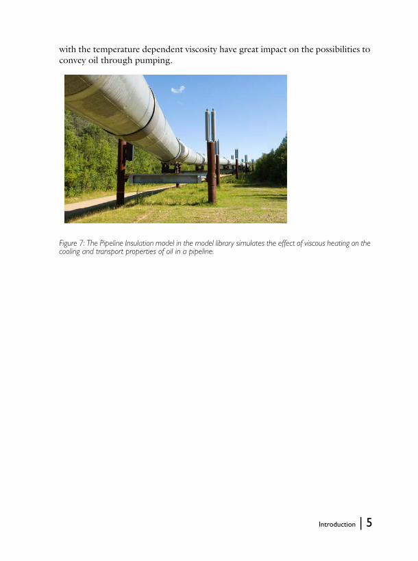
with the temperature dependent viscosity have great impact on the possibilities to convey oil through pumping.

Figure 7: The Pipeline Insulation model in the model library simulates the effect of viscous heating on the cooling and transport properties of oil in a pipeline.

Introduction | 5

The Pipe Flow Module Interfaces

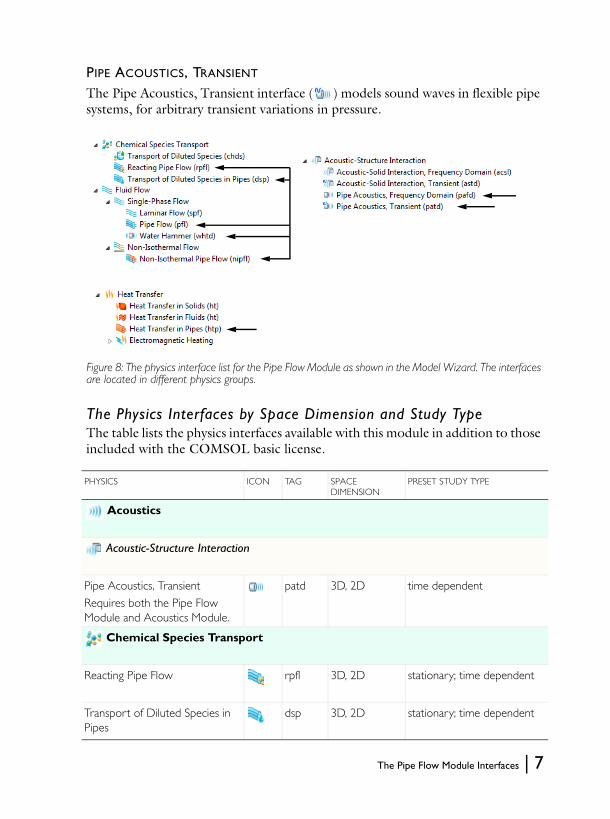
The module includes the following physics interfaces. See also the graphical view from the Model Wizard, shown in Figure 8 on page 7.

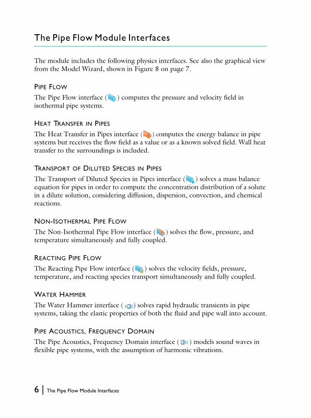
PIPE FLOW

The Pipe Flow interface ( ) computes the pressure and velocity field in isothermal pipe systems.

HEAT TRANSFER IN PIPES

The Heat Transfer in Pipes interface ( ) computes the energy balance in pipe systems but receives the flow field as a value or as a known solved field. Wall heat transfer to the surroundings is included.

TRANSPORT OF DILUTED SPECIES IN PIPES

The Transport of Diluted Species in Pipes interface ( ) solves a mass balance equation for pipes in order to compute the concentration distribution of a solute in a dilute solution, considering diffusion, dispersion, convection, and chemical reactions.

NON-ISOTHERMAL PIPE FLOW

The Non-Isothermal Pipe Flow interface ( ) solves the flow, pressure, and temperature simultaneously and fully coupled.

REACTING PIPE FLOW

The Reacting Pipe Flow interface ( ) solves the velocity fields, pressure, temperature, and reacting species transport simultaneously and fully coupled.

WATER HAMMER

The Water Hammer interface ( ) solves rapid hydraulic transients in pipe systems, taking the elastic properties of both the fluid and pipe wall into account.

PIPE ACOUSTICS, FREQUENCY DOMAIN

The Pipe Acoustics, Frequency Domain interface ( ) models sound waves in flexible pipe systems, with the assumption of harmonic vibrations.

6 | The Pipe Flow Module Interfaces

PIPE ACOUSTICS, TRANSIENT

The Pipe Acoustics, Transient interface ( ) models sound waves in flexible pipe systems, for arbitrary transient variations in pressure.

Figure 8: The physics interface list for the Pipe Flow Module as shown in the Model Wizard. The interfaces are located in different physics groups.

The Physics Interfaces by Space Dimension and Study TypeThe table lists the physics interfaces available with this module in addition to those included with the COMSOL basic license.

PHYSICS ICON TAG SPACE DIMENSION

PRESET STUDY TYPE

Acoustics

Acoustic-Structure Interaction

Pipe Acoustics, Transient

Requires both the Pipe Flow Module and Acoustics Module.

patd 3D, 2D time dependent

Chemical Species Transport

Reacting Pipe Flow rpfl 3D, 2D stationary; time dependent

Transport of Diluted Species in Pipes

dsp 3D, 2D stationary; time dependent

The Pipe Flow Module Interfaces | 7

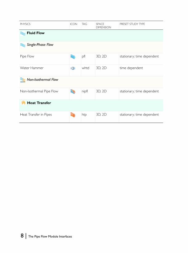
Fluid Flow

Single-Phase Flow

Pipe Flow pfl 3D, 2D stationary; time dependent

Water Hammer whtd 3D, 2D time dependent

Non-Isothermal Flow

Non-Isothermal Pipe Flow nipfl 3D, 2D stationary; time dependent

Heat Transfer

Heat Transfer in Pipes htp 3D, 2D stationary; time dependent

PHYSICS ICON TAG SPACE DIMENSION

PRESET STUDY TYPE

8 | The Pipe Flow Module Interfaces

The Model Libraries Window

To open a Pipe Flow Module model library model, click Blank Model in the New screen. Then on the Home or Main toolbar click Model Libraries . In the Model Libraries window that opens, expand the Pipe Flow Module folder and browse or search the contents. Click Open Model to open the model in COMSOL Multiphysics or click Open PDF Document to read background about the model including the step-by-step instructions to build it. The MPH-files in the COMSOL model library can have two formats—Full MPH-files or Compact MPH-files.• Full MPH-files, including all meshes and solutions. In the Model Libraries

window these models appear with the icon. If the MPH-file’s size exceeds 25MB, a tip with the text “Large file” and the file size appears when you position the cursor at the model’s node in the Model Libraries tree.

• Compact MPH-files with all settings for the model but without built meshes and solution data to save space on the DVD (a few MPH-files have no solutions for other reasons). You can open these models to study the settings and to mesh and re-solve the models. It is also possible to download the full versions—with meshes and solutions—of most of these models when you update your model library. These models appear in the Model Libraries window with the icon. If you position the cursor at a compact model in the Model Libraries window, a No solutions stored message appears. If a full MPH-file is available for download, the corresponding node’s context menu includes a Download Full Model item ( ).

To check all available Model Libraries updates, select Update COMSOL Model Library ( ) from the File>Help menu (Windows users) or from the Help menu (Mac and Linux users). The next section uses a model from the model library. Go to “Tutorial Example: Geothermal Heating from a Pond Loop” to get started.

The Model Libraries Window | 9

Tutorial Example: Geothermal Heating from a Pond Loop

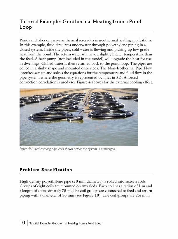
Ponds and lakes can serve as thermal reservoirs in geothermal heating applications. In this example, fluid circulates underwater through polyethylene piping in a closed system. Inside the pipes, cold water is flowing and picking up low grade heat from the pond. The return water will have a slightly higher temperature than the feed. A heat pump (not included in the model) will upgrade the heat for use in dwellings. Chilled water is then returned back to the pond loop. The pipes are coiled in a slinky shape and mounted onto sleds. The Non-Isothermal Pipe Flow interface sets up and solves the equations for the temperature and fluid flow in the pipe system, where the geometry is represented by lines in 3D. A forced convection correlation is used (see Figure 4 above) for the external cooling effect.

Figure 9: A sled carrying pipe coils shown before the system is submerged.

Problem Specif ication

High density polyethylene pipe (20 mm diameter) is rolled into sixteen coils. Groups of eight coils are mounted on two sleds. Each coil has a radius of 1 m and a length of approximately 75 m. The coil groups are connected to feed and return piping with a diameter of 50 mm (see Figure 10). The coil groups are 2.4 m in

10 | Tutorial Example: Geothermal Heating from a Pond Loop

height and sit at the bottom of a pond that is 6 m deep. The total length of the piping is 1446 m.

Figure 10: Polyethylene pipe system. Elevation above the pond bottom is indicated. Feed and return piping (gray) is 50 mm in diameter while coils (black) are 20 mm in diameter.

The heat exchange between pond water and pipe fluid will depend, among other things, on the temperature difference between the two. A slow current in the pond will make the heat transfer more effective than water at rest. The pond is warmer closer to the surface, as shown by the temperature data in the table below.

POND TEMPERATURE

Elevation (m) Temperature (K)

0 284

2 288

4 291

6 293

2.4 m

2 m

6 m9 m

9 m

2.4 m

2.4 m

0 m

0 m

feedreturn

Tutorial Example: Geothermal Heating from a Pond Loop | 11

It is easy to set up a function in the software with linear interpolation between points so that the varying pond temperature can be taken into account in the simulation.

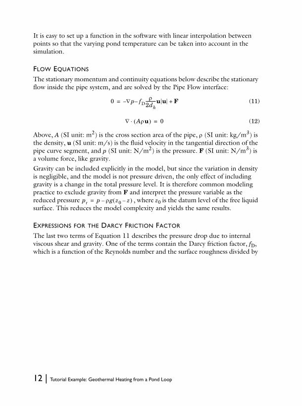
FLOW EQUATIONS

The stationary momentum and continuity equations below describe the stationary flow inside the pipe system, and are solved by the Pipe Flow interface:

(11)

(12)

Above, A (SI unit: m2) is the cross section area of the pipe, (SI unit: kg/m3) is the density, u (SI unit: m/s) is the fluid velocity in the tangential direction of the pipe curve segment, and p (SI unit: N/m2) is the pressure. F (SI unit: N/m3) is a volume force, like gravity.Gravity can be included explicitly in the model, but since the variation in density is negligible, and the model is not pressure driven, the only effect of including gravity is a change in the total pressure level. It is therefore common modeling practice to exclude gravity from F and interpret the pressure variable as the reduced pressure , where z0 is the datum level of the free liquid surface. This reduces the model complexity and yields the same results.

EXPRESSIONS FOR THE DARCY FRICTION FACTOR

The last two terms of Equation 11 describes the pressure drop due to internal viscous shear and gravity. One of the terms contain the Darcy friction factor, fD, which is a function of the Reynolds number and the surface roughness divided by

0 p– fD

2dh----------u u– F+=

Au 0=

pr p g z0 z– –=

12 | Tutorial Example: Geothermal Heating from a Pond Loop

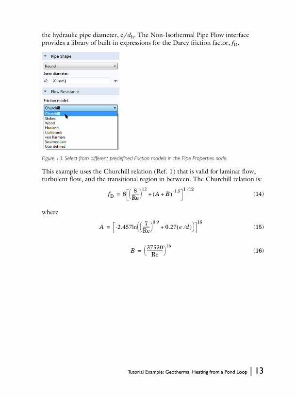
the hydraulic pipe diameter, e/dh. The Non-Isothermal Pipe Flow interface provides a library of built-in expressions for the Darcy friction factor, fD.

Figure 13: Select from different predefined Friction models in the Pipe Properties node.

This example uses the Churchill relation (Ref. 1) that is valid for laminar flow, turbulent flow, and the transitional region in between. The Churchill relation is:

(14)

where

(15)

(16)

fD 8 8Re------- 12

A B+ -1.5+

1 12=

A -2.457ln 7Re------- 0.9

0.27 e d + 16

=

B 37530Re

---------------- 16

=

Tutorial Example: Geothermal Heating from a Pond Loop | 13

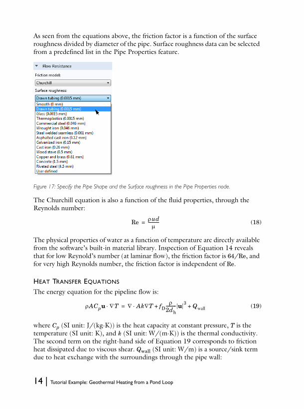
As seen from the equations above, the friction factor is a function of the surface roughness divided by diameter of the pipe. Surface roughness data can be selected from a predefined list in the Pipe Properties feature.

Figure 17: Specify the Pipe Shape and the Surface roughness in the Pipe Properties node.

The Churchill equation is also a function of the fluid properties, through the Reynolds number:

(18)

The physical properties of water as a function of temperature are directly available from the software’s built-in material library. Inspection of Equation 14 reveals that for low Reynold’s number (at laminar flow), the friction factor is 64/Re, and for very high Reynolds number, the friction factor is independent of Re.

HEAT TRANSFER EQUATIONS

The energy equation for the pipeline flow is:

(19)

where Cp (SI unit: J/(kg·K)) is the heat capacity at constant pressure, T is the temperature (SI unit: K), and k (SI unit: W/(m·K)) is the thermal conductivity. The second term on the right-hand side of Equation 19 corresponds to friction heat dissipated due to viscous shear. Qwall (SI unit: W/m) is a source/sink term due to heat exchange with the surroundings through the pipe wall:

Re ud

-----------=

ACpu T Ak T fD+

2dh---------- u 3 Qwall+=

14 | Tutorial Example: Geothermal Heating from a Pond Loop

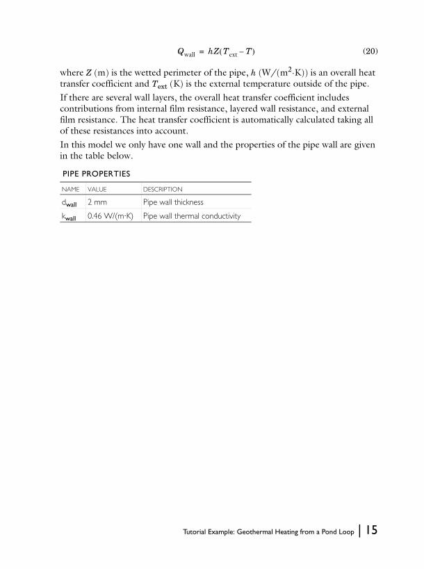
(20)

where Z (m) is the wetted perimeter of the pipe, h (W/(m2·K)) is an overall heat transfer coefficient and Text (K) is the external temperature outside of the pipe. If there are several wall layers, the overall heat transfer coefficient includes contributions from internal film resistance, layered wall resistance, and external film resistance. The heat transfer coefficient is automatically calculated taking all of these resistances into account.In this model we only have one wall and the properties of the pipe wall are given in the table below.

PIPE PROPERTIES

NAME VALUE DESCRIPTION

dwall 2 mm Pipe wall thickness

kwall 0.46 W/(m·K) Pipe wall thermal conductivity

Qwall hZ Text T– =

Tutorial Example: Geothermal Heating from a Pond Loop | 15

Results

Figure 21 shows the pressure (Pa) in the 1446 m pipe system assuming that water enters the system at a rate of 4 l/s.

Figure 21: Pressure drop over the pipe system due to flow losses.

16 | Tutorial Example: Geothermal Heating from a Pond Loop

The plot below shows the temperature (K) distribution for the pipe fluid. It enters the pipe system at 5 °C and exits with a temperature of approximately 11 °C.

Figure 22: Temperature of the pipe fluid.

Turbulent flow conditions in the loop are important for good heat exchange between the pipes and the surroundings. A plot of the Reynolds number is shown in Figure 23, confirming that flow is turbulent (Re > 3000) throughout the

Tutorial Example: Geothermal Heating from a Pond Loop | 17

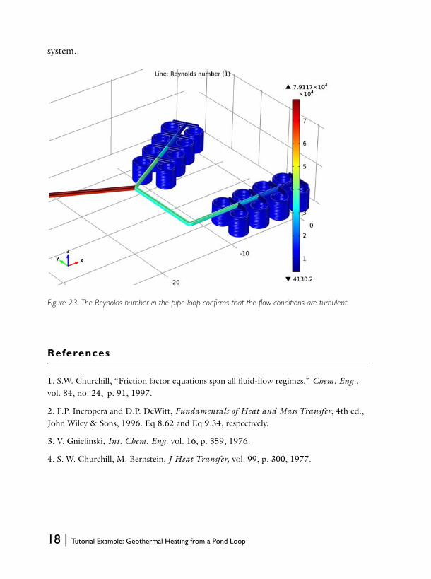
system.

Figure 23: The Reynolds number in the pipe loop confirms that the flow conditions are turbulent.

References

1. S.W. Churchill, “Friction factor equations span all fluid-flow regimes,” Chem. Eng., vol. 84, no. 24, p. 91, 1997.

2. F.P. Incropera and D.P. DeWitt, Fundamentals of Heat and Mass Transfer, 4th ed., John Wiley & Sons, 1996. Eq 8.62 and Eq 9.34, respectively.

3. V. Gnielinski, Int. Chem. Eng. vol. 16, p. 359, 1976.

4. S. W. Churchill, M. Bernstein, J Heat Transfer, vol. 99, p. 300, 1977.

18 | Tutorial Example: Geothermal Heating from a Pond Loop

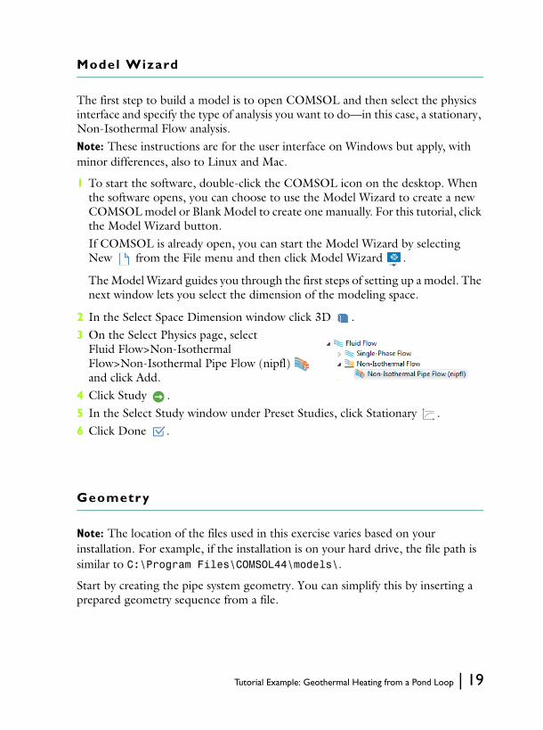
Model Wizard

The first step to build a model is to open COMSOL and then select the physics interface and specify the type of analysis you want to do—in this case, a stationary, Non-Isothermal Flow analysis.Note: These instructions are for the user interface on Windows but apply, with minor differences, also to Linux and Mac.

1 To start the software, double-click the COMSOL icon on the desktop. When the software opens, you can choose to use the Model Wizard to create a new COMSOL model or Blank Model to create one manually. For this tutorial, click the Model Wizard button.If COMSOL is already open, you can start the Model Wizard by selecting New from the File menu and then click Model Wizard .

The Model Wizard guides you through the first steps of setting up a model. The next window lets you select the dimension of the modeling space.

2 In the Select Space Dimension window click 3D .3 On the Select Physics page, select

Fluid Flow>Non-Isothermal Flow>Non-Isothermal Pipe Flow (nipfl) and click Add.

4 Click Study .5 In the Select Study window under Preset Studies, click Stationary .6 Click Done .

Geometry

Note: The location of the files used in this exercise varies based on your installation. For example, if the installation is on your hard drive, the file path is similar to C:\Program Files\COMSOL44\models\.

Start by creating the pipe system geometry. You can simplify this by inserting a prepared geometry sequence from a file.

Tutorial Example: Geothermal Heating from a Pond Loop | 19

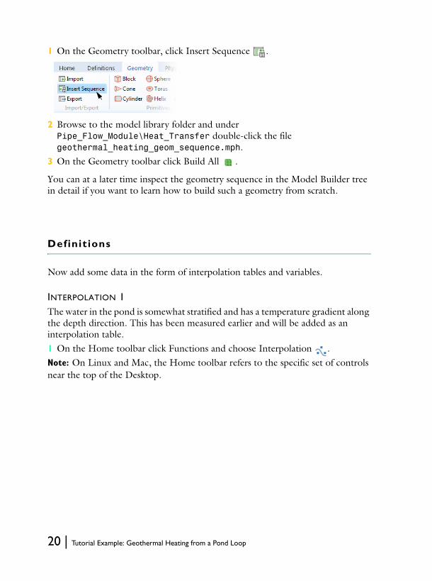
1 On the Geometry toolbar, click Insert Sequence .

2 Browse to the model library folder and under Pipe_Flow_Module\Heat_Transfer double-click the file geothermal_heating_geom_sequence.mph.

3 On the Geometry toolbar click Build All .

You can at a later time inspect the geometry sequence in the Model Builder tree in detail if you want to learn how to build such a geometry from scratch.

Definit ions

Now add some data in the form of interpolation tables and variables.

INTERPOLATION 1The water in the pond is somewhat stratified and has a temperature gradient along the depth direction. This has been measured earlier and will be added as an interpolation table.1 On the Home toolbar click Functions and choose Interpolation . Note: On Linux and Mac, the Home toolbar refers to the specific set of controls near the top of the Desktop.

20 | Tutorial Example: Geothermal Heating from a Pond Loop

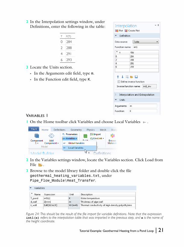
2 In the Interpolation settings window, under Definitions, enter the following in the table:

3 Locate the Units section. - In the Arguments edit field, type m.- In the Function edit field, type K.

VARIABLES 11 On the Home toolbar click Variables and choose Local Variables .

2 In the Variables settings window, locate the Variables section. Click Load from File .

3 Browse to the model library folder and double-click the file geothermal_heating_variables.txt, under Pipe_Flow_Module\Heat_Transfer.

Figure 24: This should be the result of the file import for variable definitions. Note that the expression int1(z) refers to the interpolation table that was imported in the previous step, and z is the name of the height coordinate.

T F(T)

0 284

2 288

4 291

6 293

Tutorial Example: Geothermal Heating from a Pond Loop | 21

Materials

1 On the Home toolbar click Add Material .2 In the tree, select Built-In>Water, liquid.3 Click Add to Component.

Non-Isothermal Pipe Flow

Now is the time to specify the physics settings, which include the flow and temperature conditions, as well as the pressure drop correlations to use in the pipe segments. Since piping systems typically consist of a large number of different segments, you will find it very efficient to use selections to get a manageable model.

PIPE PROPERTIES 11 In the Model Builder under Component 1>Non-Isothermal Pipe Flow, click

Pipe Properties 1.

22 | Tutorial Example: Geothermal Heating from a Pond Loop

Note: In many of the settings windows in COMSOL, there is an Equation section that you can expand (see image to the right). This shows you the equations employed by the current setting. In this case, the correlations for the default friction factor model Churchill is displayed. Also, if you are interested in the underlying theory of any settings window, press F1 or the Help button . This takes you to the documentation section describing the current settings window.

2 In the Pipe Properties settings window, locate the Pipe Shape section.- From the Shape list, choose Round.- In the di edit field, type 20[mm].

TEMPERATURE 11 In the Model Builder under Component 1>Non-Isothermal Pipe Flow

click Temperature 1.2 In the Temperature settings window, locate the Temperature section.3 In the Tin edit field, type 5[degC].

PIPE PROPERTIES 2Now you assign additional different properties to a group of pipe segments, which then deviates from the default properties added earlier.1 In the Model Builder, right-click Non-Isothermal Pipe Flow and choose

Pipe Properties.

Tutorial Example: Geothermal Heating from a Pond Loop | 23

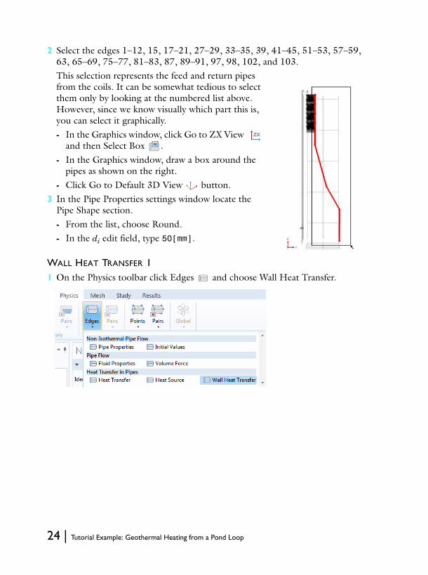
2 Select the edges 1–12, 15, 17–21, 27–29, 33–35, 39, 41–45, 51–53, 57–59, 63, 65–69, 75–77, 81–83, 87, 89–91, 97, 98, 102, and 103.This selection represents the feed and return pipes from the coils. It can be somewhat tedious to select them only by looking at the numbered list above. However, since we know visually which part this is, you can select it graphically. - In the Graphics window, click Go to ZX View

and then Select Box . - In the Graphics window, draw a box around the

pipes as shown on the right. - Click Go to Default 3D View button.

3 In the Pipe Properties settings window locate the Pipe Shape section. - From the list, choose Round.- In the di edit field, type 50[mm].

WALL HEAT TRANSFER 11 On the Physics toolbar click Edges and choose Wall Heat Transfer.

24 | Tutorial Example: Geothermal Heating from a Pond Loop

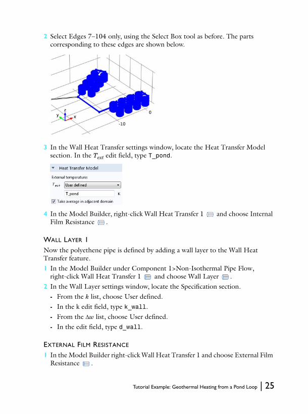
2 Select Edges 7–104 only, using the Select Box tool as before. The parts corresponding to these edges are shown below.

3 In the Wall Heat Transfer settings window, locate the Heat Transfer Model section. In the Text edit field, type T_pond.

4 In the Model Builder, right-click Wall Heat Transfer 1 and choose Internal Film Resistance .

WALL LAYER 1Now the polyethene pipe is defined by adding a wall layer to the Wall Heat Transfer feature.1 In the Model Builder under Component 1>Non-Isothermal Pipe Flow,

right-click Wall Heat Transfer 1 and choose Wall Layer .2 In the Wall Layer settings window, locate the Specification section.

- From the k list, choose User defined.- In the k edit field, type k_wall.- From the w list, choose User defined.- In the edit field, type d_wall.

EXTERNAL FILM RESISTANCE 1 In the Model Builder right-click Wall Heat Transfer 1 and choose External Film

Resistance .

Tutorial Example: Geothermal Heating from a Pond Loop | 25

2 In the External Film Resistance settings window, locate the Specification section.- In the External film heat transfer model

list, External forced convection should now be active by default.

- From the External material list, choose Water, liquid.

- In the uext edit field, type 0.2[m/s].

The external slow flow of 0.2 m/s is the mild current in the pond. This is enough to consider it forced convection outside the tubes. The temperature dependent material properties of water are all taken from the Materials node as added earlier.

Figure 25: More than one Wall Layer can be added if you want a multilayered pipe wall.

INLET 11 On the Physics toolbar click Points and choose Inlet .2 Select Point 1 only.3 In the Inlet settings window, locate the Inlet Specification section.

- From the Specification list, choose Volumetric flow rate.- In the qv,0 edit field, type 4[l/s] (as in liters/second).

HEAT OUTFLOW 11 On the Physics toolbar click Points and choose Heat Outflow .2 Select Point 2 only.

26 | Tutorial Example: Geothermal Heating from a Pond Loop

Mesh

1 In the Model Builder under Component 1, click Mesh 1 .

2 In the Mesh settings window, locate the Mesh Settings section.3 From the Element size list, choose Extremely fine.4 Click the Build All button .5 Click the Go to Default 3D View button on the Graphics toolbar.

Solve

On the Home toolbar click Compute .

View the Results

PRESSURE

The default plot groups show the pressure (Figure 21), velocity, and temperature (Figure 22) in the pipe system. To get a better view, do as follows:1 Click the Zoom Box button on the Graphics toolbar.

Tutorial Example: Geothermal Heating from a Pond Loop | 27

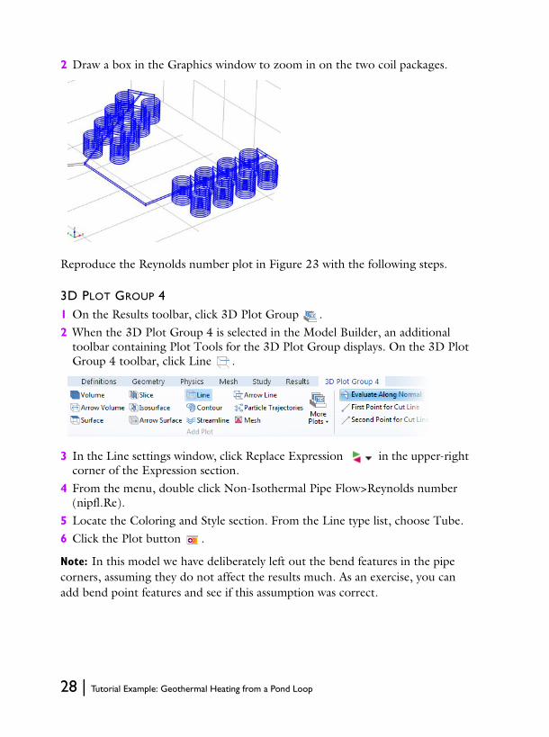
2 Draw a box in the Graphics window to zoom in on the two coil packages.

Reproduce the Reynolds number plot in Figure 23 with the following steps.

3D PLOT GROUP 41 On the Results toolbar, click 3D Plot Group . 2 When the 3D Plot Group 4 is selected in the Model Builder, an additional

toolbar containing Plot Tools for the 3D Plot Group displays. On the 3D Plot Group 4 toolbar, click Line .

3 In the Line settings window, click Replace Expression in the upper-right corner of the Expression section.

4 From the menu, double click Non-Isothermal Pipe Flow>Reynolds number (nipfl.Re).

5 Locate the Coloring and Style section. From the Line type list, choose Tube.6 Click the Plot button .

Note: In this model we have deliberately left out the bend features in the pipe corners, assuming they do not affect the results much. As an exercise, you can add bend point features and see if this assumption was correct.

28 | Tutorial Example: Geothermal Heating from a Pond Loop