Introduction to the IUCN Red List of Ecosystems Categories ... · Introduction to the IUCN Red List of Ecosystems Categories and Criteria International Union for Conservation of Nature

Introduction to the IUCN Red List of Ecosystems Categories and Criteria

International Union for Conservation of Nature

Course Manual

Version 1.0

Introduction to the IUCN Red List of Ecosystems Categories and

Criteria: course manual.Murray, N.J., Miller, R.M., Zager, I., Keith, D.A., Bland, L.M., Esteves, R., Oliveira-Miranda, M.A.,

Rodríguez, J.P

http://www.iucnrle.org/

ii | IUCN Red List of Ecosystems

IUCN Red List of Ecosystems

Web www.iucnrle.org

Email Rebecca Miller ([email protected])

Nicholas Murray ([email protected])

Irene Zager ([email protected])

Citation:

Murray, N.J., Miller, R.M., Zager, I., Keith, D.A., Bland, L.M., Esteves, R., Oliveira-Miranda, M.A.,

Rodríguez, J.P. (2016) Introduction to the IUCN Red List of Ecosystems Categories and Criteria:

course manual. Downloadable from www.iucnrle.org


mailto:[email protected]




1 | IUCN Red List of Ecosystems

1. RLE Training Course ......................................................................................................... 2

1.1 Structure of this course ............................................................................................... 2

1.2 Tools and resources .................................................................................................... 2

2. Exercises: Day 1 ............................................................................................................... 4

2.1 Mapping an ecosystem................................................................................................ 4

2.2 Some caution required ................................................................................................ 6

2.3 Importing data ............................................................................................................. 7

2.4 Projection .................................................................................................................... 8

2.5 Assessing an ecosystem ............................................................................................. 9

3. Criterion A. Reduction in geographic distribution ............................................................. 10

3.1 Calculating ecosystem areas ..................................................................................... 10

3.2 Calculating rates of declines ...................................................................................... 12

3.3 Making an assessment under Criterion A .................................................................. 13

3.4 Extra exercise ........................................................................................................... 15

4. Criterion B. Restricted Geographic Distribution ............................................................... 16

4.1 Standardised measures of geographic distribution .................................................... 16

4.2 Measuring the EOO ................................................................................................... 16

4.3 Measuring the AOO ................................................................................................... 18

4.4 Continuing declines (Subcriteria B1a, B1b, B2a, B2b) ............................................... 26

4.5 Locations (Subcriteria B1c, B2c, B3) ......................................................................... 27

4.6 Extra exercises .......................................................................................................... 28

Oyster Beds of the species Ostrea edulis..................................................................... 28

Northern Sea Sponge Aggregations ............................................................................. 31

5. Exercises: Day 2 ............................................................................................................. 33

5.1 Understanding relative severity ................................................................................. 33

6. Criterion C. Environmental degradation ........................................................................... 34

6.1 Digitising data from published studies ....................................................................... 34

6.2 Calculating relative severity ....................................................................................... 35

6.3 Extra exercises (Criterion C) ..................................................................................... 37

Karst rising-spring wetland community of south east South Australia ........................... 37

7. Criterion D. Biotic processes ........................................................................................... 38

7.1 Extra exercises (Criteria C + D) ................................................................................. 38

Montane mossy temperate forest ................................................................................. 38

Snowmelt herbfields (Criterion C and D) ...................................................................... 40

8. References ..................................................................................................................... 41

9. Appendices ..................................................................................................................... 42

9.1 Answers to the exercises ........................................................................................... 42

9.2 R Code for RLE Assessments ................................................................................... 44


Welcome to the training course for the introduction of the IUCN Red List of Ecosystems

Categories and Criteria. We will work through a range of exercises supported by lectures

over the next few days, with the aim of providing an in-depth introduction to all aspects of the

IUCN Red List of Ecosystems required to complete an assessment of one or more

ecosystems. This training course is intended to be accompanied by the Guidelines for the

application of IUCN Red List of Ecosystems Categories and Criteria, which is the definitive

source for all information required to ensure consistent application of the criteria (Bland et

al., 2016).

The training course and course manual are intended as a self-learning exercise which is

supported by experts in ecosystem risk assessment. Our course will follow the general

process for assessing ecosystems as depicted in Figure 1. We will begin with a series of

introductory lectures that provides the history, background and purpose of the IUCN Red List

of Ecosystems (RLE). Following this, we will develop the theoretical basis for assessing

ecosystems under the RLE categories and criteria, allowing us to (i) define an ecosystem

type under assessment, (ii) identify and describe the key features and processes of the

ecosystem, (iii) map the distribution of the ecosystem type and (iv) collect the data

necessary for submitting to the IUCN for publication.

The remainder of the course will follow a series of lectures and practical exercises to ensure

a thorough understanding of the application of the categories and criteria. Using a case

study provided by the course instructors, we will then work through each of the criteria,

enabling us to assess the ecosystem type with a range of tools and resources. You may

wish to use your own dataset to complete these exercises. If you move quickly or have no

access to ArcGIS, we provide extra material at the end of each chapter which can be worked

through in your own time.

Lastly, we will determine the final outcome of the ecosystem risk assessment, enabling a

final classification of the status of the focal ecosystem. At all times we will allow time for

questions, discussion and you can feel free to contact us by email.

In this course we provide a range of tools and resources for completing a Red List of

Ecosystems assessment (available from iucnrle.org). The main tools we will use include:

1. ArcGIS. Optional to use QGIS, Grass or some other open source software. We are

working towards extending our documentation to include open-source software.

2. Microsoft Excel or Google Spreadsheets.

3. We also use R and Python for many of the analyses. For analytical tools and

functions written in these programming languages please go to:

https://github.com/nick-murray

http://iucnrle.org/static/media/uploads/references/key%20documents/bland-etal-2016_iucn_rle_guidelines_v1.pdf

http://iucnrle.org/static/media/uploads/references/key%20documents/bland-etal-2016_iucn_rle_guidelines_v1.pdf



Figure 1. Process for assessing the risk of collapse of an ecosystem type.

Red List of Ecosystems Assessment Criteria

Criterion A B C D E Overall

Subcriterion 1 A1: B1a: C1: D1: E:

B1b:

B1c:

Subcriterion 2 A2a: B2a: C2a: D2a:

A2b: B2b: C2b: D2b:

B2c:

Subcriterion 3 A3: B3: C3: D3:

Table 1. Overall assessment table. Fill this table out as you work through the exercises in this

book.


We will begin the exercises with a preliminary analysis of a dataset depicting the spatial

distribution of an ecosystem type. This assumes that we have fully defined our focal

ecosystem type, its characteristic native biota and abiotic environment, and have a good

understanding of the key drivers that influence the ecosystem type. As we have discussed in

the first lectures of the course, much of this information will be based on your own expertise

of the ecosystem type, a detailed literature review of published and grey literature,

discussion with experts, and clarification with experts on ecosystem risk assessment.

In this course we will not undertake any remote sensing, vegetation classifications, map

digitization or any other work required for mapping an ecosystem type. Instead, we will use a

time series dataset that was the foundation of the RLE assessment of the Tidal Flats of the

Yellow Sea (Murray et al., 2015). The details of the mapping methods have been reported in

several scientific publications (Murray et al., 2014a, Murray & Fuller, 2015, Murray et al.,

2015, Murray et al., 2012) and the datasets are available in an online data repository

(Murray et al., 2014b).

The datasets are provided as shapefiles and raster format, but in this course we will use

shapefiles only. If you have raster data for an ecosystem type, feel free to visit our tools

website for a range of workflows that enable similar analyses of raster data

(https://github.com/nick-murray). Alternatively, it is possible to convert a raster data to

polygon (shapefile) format and follow the same workflow.

The three maps (Figure 3) that have been provided are:

1. A 1950s map of intertidal areas developed from US Army topographic maps

(1:100000)

2. A 1980s map of intertidal areas developed from Landsat TM data (originally 30m

spatial grain, generalised to 100m pixel size and converted to shapefile).

3. A 2000s map of intertidal areas developed from Landsat ETM+ data (originally 30m

spatial grain, generalised to 100m pixel size and converted to shapefile). Note that

this dataset contains stripes from a malfunction of the Landsat 7 satellite, so will only

be used for demonstration purposes only.



Figure 2. The spatial distribution of the Yellow Sea tidal flat ecosystem.

Figure 3. Example of the time-series data we will use in this course. Here, historical

topographic maps (1954) and Landsat Archive satellite imagery (1981, 2010) allowed a

standardised time-series of the area of the Yellow Sea tidal flat ecosystem to be developed

for assessment under criterion A (Murray et al., 2014a, Murray et al., 2015, Murray et al.,

2012).


As with all mapping exercises, it is essential to fully understand:

1. Where does the data come from?

2. How are the data mapped?

3. What is the resolution of the map?

4. How accurate are the maps? If the maps are inaccurate then this must be accounted

for to ensure our estimates of change are comparable over time, rather than an

artefact of mapping inaccuracies.

Here, we note a few key considerations to ensure the data are directly comparable for time-

series mapping:

1. A masking procedure was applied to the three datasets to ensure all areas were

mapped with the same effort. Masks of areas afflicted with clouds and ice-cover, as

well as stripes in the post 2000 dataset (caused by a malfunction on Landsat 7), have

been applied to all three datasets, ensuring we have complete coverage for all three

time periods.

2. The datasets were generalised to a common spatial grain (resolution) of 100m pixel

size to ensure the three datasets are directly comparable.

3. The minimum patch size of each dataset was considered. As the dataset contains

maps from two different sources (topographical maps and satellite data), it is

important to understand whether one data source is able to map smaller patches

than others. In our case, a post-processing procedure ensured that very small

patches (such as single pixels) were removed (Murray & Fuller, 2012, Murray et al.,

2014b).

4. All datasets are in the same equal area projection.

5. The datasets have accuracy assessments indicating that the remote sensing derived

data are highly accurate (Murray et al., 2014a).

6. The data have been published in several peer-reviewed publications. Therefore, we

assume the methods and analysis of these datasets are to the highest standard.

After checking for these important factors, we are satisfied that the dataset is suitable for our

purposes, avoiding some common mistakes with time-series mapping (see Section 5,

guidelines). For further consideration of these common mistakes and how to avoid them,

refer to these papers:

Fuller, R. M., Smith, G. M. & Devereux, B. J. 2003. The characterisation and measurement

of land cover change through remote sensing: problems in operational applications?

International Journal of Applied Earth Observation and Geoinformation, 4, 243-253.

Olofsson, P., Foody, G. M., Herold, M., Stehman, S. V., Woodcock, C. E. & Wulder, M. A.

2014. Good practices for estimating area and assessing accuracy of land change. Remote

Sensing of Environment, 148, 42-57.


Olofsson, P., Foody, G. M., Stehman, S. V. & Woodcock, C. E. 2013. Making better use of

accuracy data in land change studies: Estimating accuracy and area and quantifying

uncertainty using stratified estimation. Remote Sensing of Environment, 129, 122-131.

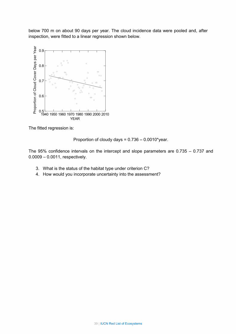
Import datasets into ArcGIS:

1. Unzip and save the provided datasets to a simple working folder, such as C:\RLE.

2. Open ArcMap. If an automatic window opens for selecting an existing project, choose

cancel to begin with an untitled project.

3. Use Add Data to add the two datasets (1950s_TidalFlat.shp and

1980s_TidalFlat.shp) using the toolbar button or via the file menu

OR

4. You can now check the datasets in detail, ideally against satellite imagery or other

high resolution data suitable for the purpose. This can be achieved in ArcGIS using

Add Basemap in the Add Data menu and selecting imagery, as long as you have the

necessary license. If your ArcGIS doesn’t have a license for this however, consider

using Google Maps, Bing Maps, USGS Landsat Look or another online satellite

imagery source.


To ensure consistency across all of the datasets, we must first check that the two datasets

have the same projection.

1. Right click the shapefile in the table of contents and select properties (if table of

contents is not visible, click the Windows menu and select Table of Contents). Click

the Source tab.

2. Ensure that both datasets are in the same projection. In this case it should be:

Projected Coordinate System: Asia_North_Albers_Equal_Area_Conic

3. If they are not the same, then reproject one or both of the datasets to a common

projection suitable for the region. This can be achieved by selecting Search For Tools

from the Geoprocessing menu. Search for “project” and select a reproject tool

(Project, Project Raster, Batch Project). If the dataset has no projection you will need

to define the projection (Define Projection) after you have first discovered which

projection the data was originally collected in.

4. In our case, our datasets have a common Albers Equal Area projection, which is

suitable for determining areas, mapping the EOO and assessing the AOO as

required for assessing against Criteria A and B of the RLE.


A summary table for each ecosystem type reports the assessment outcome for all criteria

(and subcriteria) as well as the overall status. Results for all four subcriteria of criteria A, C,

and D must be reported during the assessment process.

To account for uncertainty in the outcome of an RLE assessment, we primarily use bounded

estimates. The lower bound of the overall status is the highest lower bound (or the most

plausible value) across any of the subcriteria that return the same category as the overall

status. The upper bound of the overall status is the highest upper bound across any of the

subcriteria that return the same category as the overall status. Please see the Guidelines for

more information.

Throughout this course please complete for each example the final assessment (with

plausible bounds if required) for each ecosystem type. Please note that these examples do

not distinguish subcriteria 2a and 2b in their reporting (Tables 2 and 3).

Overall assessment table of Caribbean coral reefs


Subcriterion 1 DD LC NE EN (VU-CR) NE EN(VU-CR)

Subcriterion 2 DD LC NE DD

Subcriterion 3 DD LC NE EN

Overall assessment table of Coastal Sandstone Upland Swamps of South-Eastern Australia


Subcriterion 1 LC EN LC NT(NT-VU) DD EN(EN-CR)

Subcriterion 2 EN(EN-CR) EN EN(EN-CR) DD

Subcriterion 3 LC LC DD DD


Criterion A focuses on the decline of the geographic distribution over time. We define

geographic distribution as all spatial occurrences of an ecosystem type, which we typically

determine with an ecosystem map. When the area of an ecosystem distributions falls to

zero—when no occurrences of the ecosystem type remains—the ecosystem is considered

collapsed (Bland et al., 2016).

The RLE allows assessment of ecosystems over a range of timeframes. Owing to a failure of

a sensor on Landsat 7 (ETM+) in 2002, the mapping exercise for the 2000s is more difficult

and required use of data masks and several processing steps to achieve robust change

estimates (Murray et al., 2014a). Therefore, in this course we will demonstrate area

calculations on the 1950s and 1980s dataset only, and provide you with the area obtained

from the 2000s dataset.

As described in Section 2.2, we should first check that the datasets are fit-for-purpose in

making comparisons of area (see suggested reading from section 2).

1. What resolution is each dataset recorded at? Record it

a. Read the metadata if it is a shapefile to understand the source of the data.

This has been provided for the 1950s dataset.

b. For raster data (.tif, .img, etc), use Get Raster Properties tool in ArcGIS for

raster data.

2. If the data is of different pixel resolution, we must generalise it to a common

resolution to ensure our analysis is not biased. There are many ways to achieve this,

but most commonly used are resampling methods. Some precautions should be

made with this and, if this is a problem with your datasets, we ask you to refer to the

guidelines for more information on the various ways that this can be achieved (Bland

et al., 2016).

3. In our case, our two shapefiles are considered suitable for use, since we have read

the scientific papers and metadata that accompany the datasets.

We can now determine the area of the ecosystem at each point in time, recording the area

(in km2) as well as the specific year that the ecosystem was mapped.

As we are using shapefiles, we will determine the area of each dataset using tools in

ArcGIS:

1. Two methods can be used to calculate areas of shapefiles in ArcGIS:

2. First we can use the Calculate Areas (spatial statistics) tool, which outputs a new

shapefile where each polygon is given an area.

3. However, a simpler method is to use the attribute table tools as follows:

a. Right click the shapefile, select Open Attribute Table


b. Select the Table Options button

c. Click Add Field

d. Give the Name “AreaKm2”, and change the Type to “Float”. Select OK.

e. Now, right click the new column in the table and select Calculate Geometry.

Review the warning, then click yes.

f. Choose Area as the Property, change Units to Square Kilometers [sq km] and

select OK. Again you can ignore the warning.

g. You will now see that the area of the ecosystem is provided in square

kilometres within the attribute table.

4. Record the data in the table below.

5. Always double check area estimates. You can use other methods to do this, such as

using the Python and R tools provided on N. Murray’s GitHub (see supplementary

material if you wish to use these tools).


If we were using raster data, the area of ecosystems distributions can be determined by

counting the number of pixels and multiplying by their area. (see N. Murray’s GitHub).

Year Area (km2) Notes

1958

1988

2008 3893.03 Provided in Murray et al (2014)

The RLE guidelines suggest two methods to determine the rate of decline of an ecosystem,

each of which assumes a different functional form of the decline (Bland et al., 2016). In a

proportional rate of decline (PRD), the decline is a fraction of the previous year’s remaining

area (0.02 × last year’s area), while in an absolute rate of decline (ARD) the area subtracted

each year is a constant fraction of the area of the ecosystem at the beginning of the decline

(0.02 × 1000 = 20 km2/year) (Bland et al., 2016). Calculating these rates of decline allow

extrapolation to the full timeframe of an assessment (50 years in past, present or future).

The rates of decline can be calculated using our Excel spreadsheet, in R (see the resources

sections of iucnrle.org), Python (see GitHub), or simply with a calculator. Here we use the

1988 (year.t2) area estimate (area.t2) against the 1958 (year.t1) area estimate (area.t1):

1. Calculate absolute rate of decline between 1958 and 1988:

ARD = - (Area.t2 - Area.t1)/(year.t2 - year.t1)

= - (5448.5 - A.t1)/(1988-1958)

= ?

2. Calculate proportional rate of decline:

PRD = 100 x (1-(Area.t2/Area.t1)(1/(year.t2-year.t1)))

= 100 x (1-(5448.5 / A.t1) (1/ (1988-1958)

= ?


Now we have an estimate of the extent of decline of our ecosystem type. We can assess the

ecosystem against the RLE thresholds. An ecosystem may be listed under criterion A if it

meets the thresholds for any of four subcriteria (A1, A2a, A2b or A3), quantified as a

reduction in geographic distribution over the following time frames:

Subcriterion Time frame CR EN VU

A1 Past (over the past 50 years) ≥ 80% ≥ 50% ≥ 30%

A2a Future (over the next 50 years) ≥ 80% ≥ 50% ≥ 30%

A2b Future (over any 50 year period including the past,

present and future)

≥ 80% ≥ 50% ≥ 30%

A3 Historical (since approximately 1750) ≥ 90% ≥ 70% ≥ 50%

However, we only have our estimates of declines in terms of absolute areas lost for a given

timeframe. We can adjust these to a percentage reduction in area using the following

equations:

1. Calculate % area lost between time 1 and time 2:

% lost = ((Area.t1 - Area.t2)/Area.t1) × 100

= ?

Thus, as our data fits exactly a 50 year period we can use this percentage area lost to

assess under the categories and criteria to determine the status of our ecosystem under

Criterion A.

In many cases, our time frames will not fit the exact 50 year period for an assessment. In

these cases, we can use our observed absolute and proportional rates of decline to estimate

the area at a future date, equating to 50 years since our first observed data point. It will be

interesting to compare our very simple forecast with the empirical data provided in Murray et

al. (2014a).

2. Estimate area of ecosystem 50 years into the future using proportional rate of decline

assumption. Recall that area.t1 is the area in km2 of tidal flats in year.t1 (1958):

Area.2008.PRD = Area.t1 × (1 - (PRD/100))nYears

= Area.t1 × (1 –(PRD/100))50

= ?

3. Estimate area of ecosystem 50 years into the future using the assumption of an

absolute rate of decline:

Area.2008.ARD = Area.t1 – (ARD × nYears)


= Area.t1 - (ARD × 50)

= ?

Compare these results with those published in Murray et al. (2014a). We note that the

observed area of tidal flats from remote sensing data in 2008[7][7] (3893.03 km2) are

incredibly close to those estimated with a Proportional Rate of Decline assumption. For

further information on the functional forms of decline refer to the guidelines (Bland et al.,

2016).

Now, calculate the percentage area lost between 1958 and 2008:

4. Calculate % area lost between 1958 (t1) and your estimate of 2008 (t3) area derived

from the equations above (Area.2008.PRD):

% lost = ((Area.t1 - Area.2008.PRD)/Area.t1) × 100

= ?

Again, note how similar this estimate is to the empirical estimate of the loss of tidal flats

(Murray et al., 2014a).

Record the outcome of the assessment.

When there are more than two data points it is possible to apply far more advanced and

suitable statistical analysis methods to the time-series area data. We encourage assessors

to fit statistical models to the time-series data where possible, allowing full use of all data

available to achieve better estimates of the time-series area changes. Such models also

allow incorporation of further information, such as accuracy of the datasets at each time

point and covariate information that can improve model fit, and will generally result in more

accurate predictions than the methods provided here. In all cases, information on the type of

models used, the assumptions of the functional form of the decline and any other relevant

information should be included in the RLE assessment.


Two maps of land cover, which we will consider are ecosystems mapped according to the

Guidelines, have been produced around the cities of Maracay and Valencia (Figure 1),

adjacent to Lake Valencia, Venezuela (large black area at the bottom left). The land cover

maps were produced using Landsat Archive satellite images, and the area of each

ecosystem type was determined (Table 1). The ecosystem types have changed rapidly in

the last decades, and we are interested in classifying the risk of collapse of each ecosystem

type using the RLE criteria.

Change in extent of six land cover types between 1986 and 2001 in north-central Venezuela

Year 1986

(km2)

2001

(km2) ARD PRD

2051

Area

Estimate

(PRD)

%

Change

Assessment

outcome

Evergreen

forest 397 385

Semi-

deciduous

forest

1190 1037

Deciduous

forest 2227 1563

Grasslands 1249 2001

Using these area estimates, estimate the risk of collapse of the different land covers

according to Criterion A.

Terrestrial ecosystems of northern Venezuela

(2001)


Criterion B uses measures of the geographic distribution of an ecosystem type to identify

ecosystems that are at risk from catastrophic disturbances. In general, ecosystems that are

widely distributed or exist across multiple independent patches are at lower risk from

catastrophes, disturbance events or any other threats that exhibit a degree of spatial

contagion (e.g. invasions, pollution, fire, forestry operations, and hydrological or regional

climate change). The primary role of criterion B is to identify ecosystems whose distribution

is so restricted that they are at risk of collapse from the chance occurrence of single or few

interacting threatening events (Rodríguez et al., 2015). Criterion B also includes an

approximation for an estimate of occupied habitat for component biota, which is positively

related to population viability irrespective of exposure to catastrophic events

The geographic distribution of an ecosystem type is assessed under criterion B with two

standardized metrics: the extent of occurrence (EOO) and the area of occupancy (AOO)

(Gaston & Fuller, 2009, Keith et al., 2013). It must be emphasised that EOO and AOO are

not used to estimate the mapped area of an ecosystem like the methods we used in

Criterion A; they are simply spatial metrics that allow us to standardise an estimate of risk

spreading. Thus, it is critical that these measures are used consistently across all

assessments, and the use of non-standard measures invalidates comparison against the

thresholds. Refer to the guidelines for more information on AOO and EOO (Bland et al.,

2016).

As we are only interested in the risk of collapse of an extant ecosystem, we will use only the

latest spatial distribution map available for this exercise (the 2008 distribution of Yellow Sea

tidal flats).

Measure of Distribution Area (km2) Notes

AOO ?

AOO (1 per cent rule)

EOO ?

The RLE guidelines defines the EOO as:

The EOO of an ecosystem is measured by determining the area (km2) of a minimum

convex polygon—the smallest polygon that encompasses all known occurrences of a

focal ecosystem in which no internal angle exceeds 180 degrees— fitted to an

ecosystem distribution. The minimum convex polygon (also known as a convex hull)

must not exclude any areas, discontinuities or disjunctions, regardless of whether the

ecosystem can occur in those areas or not. Regions such as oceans (for terrestrial

ecosystems), land (for coastal or marine ecosystems), or areas outside the study


area (such as in a different country) must remain included within the minimum

convex polygon to ensure that this standardized method is comparable across

ecosystem types. In addition, these features contribute to spreading risks across the

distribution of the ecosystem by making different parts of its distribution more

spatially independent (Bland et al., 2016).

Thus, to accurately measure the EOO of an ecosystem we must apply a minimum convex

polygon to our ecosystem data, which can be easily achieved using ArcGIS:

1. Load the 2000’s tidal flat shapefile into ArcGIS using the procedure above, if not

already completed.

2. From the Geoprocessing menu, select Search For Tools

3. In the search box, search for Minimum Bounding Geometry.

4. Open the Minimum Bounding Geometry tool

5. As the input feature, select your 2000s tidal flat shapefile.

6. Save the output feature class to your working folder as EOO.shp

7. Under Geometry Type, select CONVEX_HULL

8. Group Option should be set as ALL

We now have a minimum convex polygon (convex hull) that encompasses all known

occurrences of the ecosystem type. Note that under no circumstances can the MCP be

modified, despite the inclusion of unsuitable areas, as it is a standardized measure of

distribution.


We must now determine the area of the minimum convex polygon, which allows us to

assess Criterion B. We use the same method as in the first exercise to determine the area of

the shapefile.

a. Right click the shapefile, select Open Attribute Table

b. Select the Table Options button

c. Click Add Field

d. Give the Name AreaKm2, and change the Type to “Float”. Select OK.

e. Now, right click the new column in the table and select Calculate Geometry.

Click yes to ignore the warning.

f. Choose Area as the Property, change Units to Square Kilometers [sq km] and

select OK. Again you can ignore the warning.

g. You will now see that the area of the ecosystem is provided in square

kilometres within the attribute table.

Record the area of the EOO in the table above.

As the primary source of all information on the RLE, the guidelines have a detailed section

on the theory, background and methods for measuring the AOO of an ecosystem type:

Area of occupancy (AOO). Measures of AOO are highly sensitive to the grain size

(pixel resolution) at which the distribution is mapped (Nicholson et al., 2009), so all

measures of AOO of an ecosystem type must be standardized to a common spatial


grain. The AOO of an ecosystem defined in the RLE is determined by counting the

number of 10 × 10 km grid cells that contain the ecosystem. This relatively large

grain size is applied for three reasons: (i) ecosystem boundaries are inherently vague

(Regan et al., 2002), so it is easier to determine that an ecosystem occurrence falls

within a larger grid cell than a smaller one; (ii) larger cells may be required to

diagnose the presence of ecosystems characterized by processes that operate over

large spatial scales, or possess diagnostic features that are sparse, cryptic, clustered

or mobile (e.g. pelagic or artesian systems); (iii) larger cells allow AOO estimation

even when high resolution distribution data are limited. Some ecosystem distributions

comprise a highly skewed distribution of patch sizes. In these cases large numbers of

small patches contribute a negligible risk-spreading effect to that of larger patches

and a correction may be applied by excluding from the AOO those grid cells that

contain patches of the ecosystem type that account for less than 1% of the grid cell

area (i.e. < 1km2 of the focal ecosystem type, Box 10). Research is in progress to

support guidance on when to apply this correction (Bland et al., 2016).

As with the EOO, it is essential that the methods used to determine the AOO of an

ecosystem type is consistent and well documented.

To measure the AOO of an ecosystem, we must first develop a suitable 10 × 10 km grid for

which to count the grid cells occupied by the ecosystem type. This is possible using standard

tools from ArcGIS:

1. Load the 2000’s tidal flat shapefile into ArcGIS using the procedure above, if not

already completed.

2. From the Geoprocessing menu, select Search For Tools.

3. In the search box, search for Create Fishnet.

4. Open the Create Fishnet (Data Management) Tool.

5. Provide a file name (10kmGrid.shp) as the Output Feature Class.

6. Use the 2000s tidal flat shapefile as the Template Extent (by dragging it in), which

limits the size of the fishnet grid.

7. Set the Cell Size Width to 10,000 m.

8. Set the Cell Size Height to 10,000 m.

9. Set the Number of Rows and Number of Columns to 0.

10. Uncheck the Create Label Point checkbox.

11. Change the Geometry Type to Polygon.

12. Click OK.


We now have a 10 × 10 km grid suitable for determining the AOO of the Yellow Sea tidal flat

ecosystem:


Now that we have the grid, it is a simple matter of counting the number of cells that intersect

it. This can be achieved in several ways, but we will use a few handy tools including select

by location:

1. First we select the grid cells that intersect our ecosystem dataset.

2. From the Selection menu, open Select By Location.

3. Set Select features from to the 10 x 10 km grid shapefile.

4. Set Source Layer to the ecosystem shapefile.

5. Set the Spatial selection method for target layer features to “intersect the source

layer feature”.

6. If default checked, uncheck the Apply a search distance box.

7. Click OK.


We now have the grid cells that intersect the ecosystem data selected:

Export this as a separate file by:

1. Right click the 10 x 10 km grid shapefile.

2. Select Data, then Export Data. This will export only the selected features of the

dataset. Call it GridSelect.shp.


3. Now we have a shapefile with 10 x 10 km grid cells that intersect our ecosystem

dataset. Since we are not using the 1% rule, we will simply count the number of grid

cells in this shapefile and use that as our AOO estimate. (Hint: use the attribute table

for this, each row is a grid cell).

However, at this stage it is important to consider the so-called 1% rule. The 1% rule is used

when a large number of small patches have negligible risk-spreading effect for the

ecosystem type. In our case, we are using tidal flats where small patches are likely to exist in

small estuaries and bays and we wish to include them in our AOO estimate.

However, in many cases small patches of habitat are more likely to have negligible impact

on risk spreading or are perhaps an artifact of mapping limitations. In those cases we use

the 1% rule. In our case, we are using tidal flats where small patches are likely to exist in

small estuaries and bays and we wish to include them in our AOO estimate. Assuming you

have ArcGIS 10.2 or greater, we must determine the amount of area of the ecosystem type

within each grid cell 10 × 10 km grid cell. We also need to determine which of these cells

contain >1 km2 of our ecosystem type. We can use a neat little built in ArcGIS tool to

determine this:

a. From the Geoprocessing menu, select Search For Tools.

b. In the search box, search for Tabulate Intersection. Note: this method only

works on ArcGIS 10.2 or greater.

c. As the Input Zone Features, use the GridSelect.shp.

d. Set the Zone Fields to FID (which is an individual identifier for each grid cell).

e. Use the ecosystem dataset as the Input Class Features.

f. Call the table TabulateIntersection.dbf.


g. Click OK.

h. Now we have a .dbf table that gives the area and percentage coverage of the

ecosystem in each individual grid cell.

i. Open the table (you can use ArcGIS by right-clicking the table in the Table of

Contents, or you can use Microsoft Excel).

j. Now it is simply a matter of determining how many grid cells are occupied by

≥ 1%. This can be done by selecting grid cells with Percentage ≥ 1%.

k. Use the Table Options menu in the top left (below Table) and choose Select

by Attribute.

l. Create a new selection by double clicking “PERCENTAGE”.

m. Add the >= operator.

n. Add the number 1, as shown below.


o. Now, click Apply and note that 373 out of 720 rows are selected. Thus our

AOO is 373 grid cells.

4. We can map this by simply using a “Join” in ArcGIS to join the

TabulateIntersection.dbf to the GridSelect.shp, using the ID columns as the common

variable, and “Area” and “Percentage” as the Join Fields. The result is a new column


in GridSelect.shp with Percentage and Area in there, which can then be selected and

exported.

5. The final result is the AOO grid cells that contain ≥1% of the ecosystem in black,

below, and the grid cells that intersect in orange.

Record the number of AOO cells in the results table above.

Now we have measured the AOO and EOO of the ecosystem, we must assess it under the

subcriteria. In our case, both metrics indicate the Yellow Sea tidal flat does not meet the

thresholds for listing under criterion B.

However, it is still necessary to consider the following information from the RLE guidelines:

To be eligible for listing under subcriteria B1 or B2, an ecosystem must meet the

EOO or AOO thresholds that delineate threat categories, as well as at least one of

three subcriteria that address various forms of decline. These subcriteria distinguish

restricted ecosystems at appreciable risk of collapse from those that persist over long

time scales within small stable ranges (Keith et al., 2013). Only qualitative evidence

of continuing decline is required to invoke the subcriteria, but relatively high

standards of evidence should be applied.

Therefore, had we met any of the Criterion B thresholds, the ecosystem could only be listed

if we had observed continuing declines, or if we expected future declines and have evidence

to support that claim.


The original published paper for the RLE assessment of the Yellow Sea tidal flats did not

report the number of locations for assessment under Criterion B (Murray et al., 2015). This

was principally due to not meeting any of the criteria and sub-criteria under B. However,

below we provide a few theoretical examples to assist in interpreting the number of locations

under Criterion B.

An ecosystem/habitat type is distributed across 10 small islands in the Galapagos Islands.

A potential threat comes from El Niño events, which impacts the entire ecosystem across

its distribution by causing substantial declines in key characteristic species. So far these

species appear to be able to recover well from these events, thus the ecosystem is able to

rebound, but if the frequency of El Niño events increases (for example, through the effects

of climate change), this may pose a serious problem to the survival of the species and

therefore the condition and stability of the ecosystem. The relationship between El Niño

and global climate change patterns is unknown, so considering El Niño as a major threat

at present may be premature. Counting the entire distribution as one location may not be

an appropriate application of the criteria.

The ecosystem is exposed to other threats, including pollution events and shifting species

composition as a result of predator introduction. Both of these threats are likely to affect

individual islands rather than the entire area in one sweep. Each island could be seen as a

location, so we conclude that the ecosystem is composed of 10 locations.

A rare habitat type occurs at 5 sites. One site occurs near an expanding urban area, and is

threatened by conversion to residential and other human uses. Two of the sites are in a rural

area and are threatened by agricultural runoff of herbicides. Two sites are in a protected

area and are not under any threat.

1. How many locations can be estimated for this ecosystem?

Locations are areas within the distribution of the ecosystem type for which one threat may

affect all localities at once. Their extent therefore depends on the nature and size of the

threat. The following figure shows a freshwater ecosystem type with two distinct spatial

occurrences: a river with a main channel that flows from top to bottom and two tributaries

that empty into the main channel, and a lake. Two plausible threats exist: introduction of an

exotic predatory fish and pollution. The red arrow indicates the point of entry of each threat.


1. Please outline the locations in the figure above and indicate the number in the space

provided.

This case study considers Ostrea beds distributed in several sites along coastlines in the

North-East Atlantic Sea. Dense beds of Ostrea oysters occur on shallow (typically 0-10m),

mostly sheltered sediments, where clean and hard substrates are available for settlement.

They also occurred in deeper waters and offshore (down to 50 m), but these beds are now

mostly depleted. Large quantities of dead oyster shell make up a substantial portion of the

substratum, supporting large numbers of other small and large marine invertebrates. Several

polychaete species are important in distinguishing this habitat type, whilst various seaweed

species are also frequently present.

The principle species in these oyster beds, Ostrea edulis, grows very large (>20 cm) and

can have a long lifespan (>20 years). Ostrea edulis is considered a keystone species given

its role in the ecology of the ecosystem type.. These functions include providing a solid

surface for settlement by other species; providing a cryptic, protective habitat that serves as

a nursery ground for small fish and other species; stabilising sediments which may in turn

provide some protection from shoreline erosion; and filtering large quantities of water.

Ostrea beds are under threat and/or decline throughout their range. Ostrea species have

been a part of the human diet for centuries, however, during the 18th and 19th centuries

fishing effort led to over-exploitation, failing recruitment, and destruction of European natural

beds, which were also affected by extremely cold winters. More recently (during the 20th

century), disease has impacted Ostrea beds, causing massive mortality and significant

population declines in European waters; populations later recovered but were replaced by

Invasive species: ___ locations Pollution: ___ locations


other species in several traditional areas. Despite new management practices and intensive

repletion programs, the production of O. edulis has remained low.

Using the maps provided:

1. Using a minimum convex polygon, draw the extent of occurrence (EOO) and estimate its

value in km2 (each cell is 10 x 10 km).

2. Calculate the area of occupancy (AOO) of this habitat type (in red):

a. Using all cells where habitat is present.

b. Excluding cells with <1% occupied.

3. Using the values of EOO and AOO calculated above, as well as the information given in

the text, please proceed to assess this habitat type against Criterion B. Each subcriterion

must be assigned a risk category. Briefly justify the assessment below, using the

information provided.

Criterion B B1 B2

B3 EOO a b c AOO a b c

Ostrea beds

Distribution of Ostrea beds considered for this exercise:



The distribution of this habitat type of sponge aggregations is restricted to an area off the

north coast of Norway. These aggregations provide habitat for 50 different species and are

found at water depths of 250-1300m where temperatures do not exceed 10°C. Sponge

communities are slow-growing and if damaged, their communities take a long time to

recover.

In the area, there has been a marked increase in bottom trawling (demersal and benthic)

and oil drilling and a documented increase in suspended sediments.

Using the map provided:

3. Using a minimum convex polygon, draw the extent of occurrence (EOO) and estimate its

size (each cell is 10 x 10 km);

4. Calculate the area of occupancy (AOO) of this habitat type (in red):

a. Using all cells where habitat is present.

b. Excluding cells with <1% occupied.

5. Using the values of EOO and AOO calculated above, please proceed to assess this

habitat type against Criterion B. Each subcriterion must be assigned a risk category.

Briefly justify the assessment below, using the information provided.

Criterion B B1 B2

B3 EOO a b c AOO a b c

Northern sea

sponge

aggregations

*fictitious habitat type and descriptions, provided for training purposes only


Map: Northern sea sponge aggregations (10x10km²)


We continue our training today on Criteria C and D. As discussed in the lectures and in detail

in the guidelines (Bland et al., 2016), Criteria C and D are defined for assessing decline in

ecosystem function or processes. These criteria focus on aspects of abiotic (environmental,

Criterion C) and biotic (Criterion D) change of an ecosystem type.

Prior to beginning these exercises, take a moment to revisit the concepts presented in the

Scientific Foundations (Section 3), the Assessment Process (Section 4) and the specific

sections for each of these criteria in the RLE guidelines (Section 5.3 and 5.4). In particular,

focus on your understanding of the selection of variables suitable for assessing the relative

severity and extent of decline. Ask your instructors if you have any questions.


To assess an ecosystem type under Criterion C, suitable variables for estimating the extent

of environmental degradation must be selected. The guidelines contain many examples for a

suite of case studies to assist in this process. Refer to Section 5.3.3 for a list of requirements

that should be met when selecting variables to assess abiotic degradation. For the Yellow

Sea tidal flat ecosystem Murray et al. (2015) used data of sediment outflow from the region’s

major rivers. The input of sediment into the Yellow Sea is considered to balance the rate of

seaward erosion, compaction and subsidence of tidal flats, thereby maintaining their areal

extent.

In this exercise we will digitise sediment flux data from a peer-reviewed paper, determine a

collapse threshold and estimate the relative severity of sediment decline.

We use sediment decline data from the Yangtze river to demonstrate how to calculate

relative severity according to the methods described in Keith et al (2013) and Rodriguez et al

(2015). The data originated as a plot in Yang et al (2005).

1. From the data folder, review the paper by Yang et al. (2005). Figures 10 and 11

present data on sediment flows from the Yangtze.

2. We will use an online application to harvest the data from this plot. Navigate to

http://arohatgi.info/WebPlotDigitizer/

3. Click on Launch App (top right)

http://arohatgi.info/WebPlotDigitizer/


4. Now, either load the Sediments_Yangtze.jpg of the plot from the data folder or drag it

into the data section of the WebPlotDigitizer.

5. Follow the instructions. It is necessary to state the type of plot and then to calibrate

the axes. Note we are using SD data (the black squares on the Y1 axis, left side of

plot) for sediment decline.

6. Now, for each point on the graph collect the data by clicking on it.

7. When all points are acquired, click view data, then export the final dataset as a .csv

Relative severity is defined as:

The estimated magnitude of past or future environmental degradation or disruption to

biotic processes, expressed as a percentage relative to a change large enough to

cause ecosystem collapse.

Relative severity describes the proportional change observed in an environmental variable

scaled between two values: one describing the initial state of the system (0%), and one

describing a collapsed state (100%). Thus, if an ecosystem type undergoes degradation with

a relative severity of 50% over an assessment time frame, this implies that that it has

transformed half way to a collapsed state.


The method for calculating the relative severity of the decline of an abiotic variable has been

described clearly in the following three papers (Bland et al., 2016, Keith et al., 2013,

Rodríguez et al., 2015). Here, we will use the method as described in the RLE guidelines,

recognizing that we do not have 50 years of data – it is useful for demonstration purposes.

However, note that this is different from the analysis published in Murray et al. (2015), which

used a least-squares regression model to estimate the severity of the decline beyond the

range of the time-series dataset.

We use a collapse threshold of zero sediment outflow, as per Murray et al. (2015). However,

for the rest of the exercise feel free to explore different thresholds to assess the sensitivity of

the method to changing the threshold of collapse.

To determine the relative severity of the observed declines of sediment outflow from the

Yangtze River:

1. Determine the sediment flow for the first and last points in our sediment dataset

(SD.t1 and SD.t2)

2. Use the following equations to rescale this variable to a proportional change:

Relative severity (%) = (Observed or predicted decline / Maximum decline) × 100

where

Observed or predicted decline = Initial value – Present or future value

and

Maximum decline = Initial value – Collapse value

3. Relative severity (%) = (SDt1 – SDt2) / (SDt1 – Collapse threshold) × 100

= (SDt1 – SDt2) / (SDt1 – 0) × 100

= __ %

Record the result.

Note that if a collapse threshold similar to the final sediment outflow would dramatically

increase how close the ecosystem is to collapsing:

4. Relative Severity = (SDt1 – SDt2) / (SD.t1 – 240) × 100

= __ %

Next, assessors determine the extent of the degradation as a proportion of the total

distribution of the ecosystem. With these two quantities assessors assign a risk category

using the described thresholds. The extent of degradation was assumed to affect the entire

Yellow Sea tidal flat ecosystem (100%). Record the outcome of this assessment.


The distinguishing feature of this ecological community is the presence of surface

expression of groundwater with sufficient head pressure to push water above the seal of the

pool resulting in flows at any given time of the year. A number of wetland plant associations

occur within the Karst Rising Spring (KRS) Wetland Community in the south east region of

South Australia. These include vegetation associations of the spring pools and those of the

peripheral peat fens. They consist of reedbeds, sedgelands, Melaleuca squarrosa

shrublands and Silky Tea-tree wet shrublands.

The principal mechanism of environmental degradation is through decline in hydrological

processes related to unsustainable extraction of groundwater, draining and global climate

change. Suitable hydrological variables for assessing criterion C include ground water

discharge volumes from spring pools and flow volume measurement from natural drainage

channels. Ground water discharge and stream flow data are available, but only for a few

sites. Drying of the springs is the most salient threat to the ecosystems because they are a

water-dependent ecosystem. Environmental degradation under criterion C may be quantified

using the daily spring discharge rate, with the collapse threshold assumed to be 30-38

megalitres per day.

Current decline:

The average flow in 2010 was estimated to be 40 ML/yr, declining from an average flow of

85.7 ML/yr in 1970. It is certain that decline in discharge commenced prior to 1970.No

information is available regarding future or historic changes in this ecosystem.

Criterion C

C1 C2 C3

Wetland community


We will not continue with an assessment of the Yellow Sea tidal flat ecosystem, as criterion

D was not assessed quantitatively due to a lack of region-wide data. It is expected that

further data synthesis, collaboration and targeted studies would allow this criterion to be

assessed adequately in the medium-term future. However, please read the paper and obtain

a good understanding of the data sources used, which included:

Observed population declines of key species, including migratory shorebirds

Increasing rate of harmful algal blooms,

Increasing rate of jellyfish blooms,

The extent and severity of plant invasions.

We provide several exercises to further your understanding of applying criteria C and D.

A mossy temperate forest occurs only on mountains higher than 700 m above sea level on

Mediterranean islands. The forest is characterised by several endemic trees, shrubs and

herbs that do not occur at lower elevations. Its stature is considerably shorter than lowland

forests on the islands, and it has a distinctive abundance and diversity of arboreal

bryophytes. The trees also support a unique arthropod assemblage.

The forest is strongly associated with a mesic microclimate. The moisture is contributed by

orographic processes, which produce significant mists and rain on the mountain tops and

upper slopes. Lower on the mountain slopes, the mossy temperate forest is replaced by pine

forests that lack the endemic trees and arboreal bryophytes. The transition takes place at

700 - 800m above sea level, and the highest mountain in the region is 900m.

1. What process is likely to pose a threat to the persistence of the mossy temperate

forests?

2. Which of the following would be the most suitable variable(s) for assessing the status

of the mossy temperate forest under criterion C?

a) Mean annual temperature

b) Mean annual rainfall

c) Cloud cover

d) Mean rainfall of the summer months

Time series data are available for weather stations on three mountains located throughout

the spatial and elevational range of the forest. These record precipitation and

presence/absence of cloud on the mountains during each day. Meteorologists from the

region advise that clouds have never been observed below 400 m elevation, and only extend


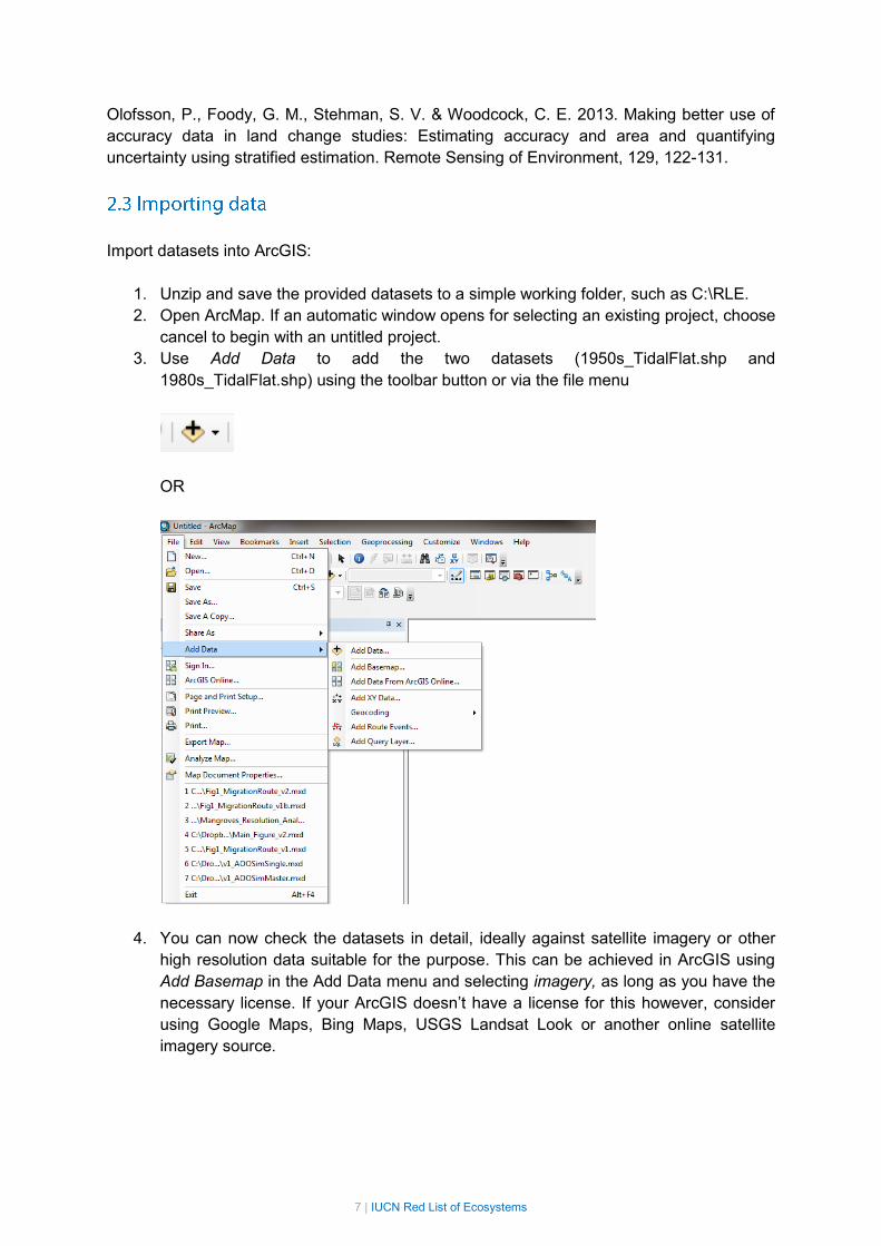
below 700 m on about 90 days per year. The cloud incidence data were pooled and, after

inspection, were fitted to a linear regression shown below.

The fitted regression is:

Proportion of cloudy days = 0.736 – 0.0010*year.

The 95% confidence intervals on the intercept and slope parameters are 0.735 – 0.737 and

0.0009 – 0.0011, respectively.

3. What is the status of the habitat type under criterion C?

4. How would you incorporate uncertainty into the assessment?

1940 1950 1960 1970 1980 1990 2000 2010

YEAR

0.5

0.6

0.7

0.8

0.9

Pro

po

rtio

n o

f C

lou

d C

ove

r D

ays p

er

Ye

ar


The highest elevated areas below permanent snow in the Alps support a unique herbfield

community. The herbfield is locally restricted to small seepage zones on flat sites and

moderate slopes, as snowmelt moisture is not retained on steeper slopes. Its occurrence is

determined by the shortest growing season tolerated by vascular plants. Sites at warmer

lower elevations and southern aspects support different assemblages dominated by mixtures

of grasses and herbs. These larger plants are able to competitively exclude the smaller

herbs at warmer temperatures, but cooler temperatures close to the permanent snowline are

beyond their physiological tolerance because the growing season is too short to allow them

to grow to maturity.

1. What processes are likely to pose a threat to the persistence of the snowmelt

herbfields?

2. Which of the following would be the most suitable variable(s) for assessing the status

of the snowmelt herbfields under criteria C and D?

a) Mean annual temperature

b) Duration of growing season

c) Depth of snow above the permanent snowline

d) Abundance of snowmelt specialist herbs at the snowline

e) Abundance of grasses in current snowmelt herbfield sites

Snowdepth time series data are available for a set of locations above the permanent

snowline throughout the range of the snowpatch herbfields. The mean winter snow depth

across the monitoring sites is currently 2.0 ± 0. 1 metres. There is no suitable habitat for

show patch herbfields at higher elevations than the snow depth monitoring sites. A linear

regression is a good fit to these data and shows that snow depth has been declining at a

rate of 0.50 to 1.0 cm per year (95% confidence interval) over the past 30 years.

3. What is a suitable threshold of snow depth that might indicate collapse of the

snowmelt herbfields? Justify your answer(s).

4. What is the estimated depth of snow 50 years from now? Can you quantify the

uncertainty in the estimate?

5. Use your answers to 3 & 4 calculate the relative severity of projected declines in

snow depth over the next 50 years. How can you quantify the uncertainty in relative

severity?

6. What is the extent of projected declines in snow depth over the next 50 years?

7. Use your answers to 5 and 6 to determine the status of snowmelt herbfield under

criterion C2.

8. Outline some limitations of this assessment, e.g. what assumptions are necessary

and how robust do you think they are?


References

Bland LM, Keith DA, Miller RM, Murray NJ, Rodríguez JP (2016) Guidelines for the application of

IUCN Red List of Ecosystems Categories and Criteria, Version 1.0. pp Page, Gland,

Switzerland, International Union for the Conservation of Nature.

Fuller RM, Smith GM, Devereux BJ (2003) The characterisation and measurement of land cover

change through remote sensing: problems in operational applications? International Journal of

Applied Earth Observation and Geoinformation, 4, 243-253.

Gaston KJ, Fuller RA (2009) The sizes of species’ geographic ranges. Journal of Applied Ecology,

46, 1-9.

Keith DA, Rodríguez JP, Brooks TM et al. (2015) The IUCN Red List of Ecosystems: Motivations,

Challenges, and Applications. Conservation Letters, 8, 214-226.

Keith DA, Rodríguez JP, Rodríguez-Clark KM et al. (2013) Scientific Foundations for an IUCN Red

List of Ecosystems. PLoS ONE, 8, e62111.

Murray NJ, Clemens RS, Phinn SR, Possingham HP, Fuller RA (2014a) Tracking the rapid loss of

tidal wetlands in the Yellow Sea. Frontiers in Ecology and the Environment, 12, 267-272.

Murray NJ, Fuller RA (2012) Coordinated effort to maintain East Asian–Australasian Flyway. Oryx,

46, 479-480.

Murray NJ, Fuller RA (2015) Protecting stopover habitat for migratory shorebirds in East Asia.

Journal of Ornithology, 156, 217-225.

Murray NJ, Ma Z, Fuller RA (2015) Tidal flats of the Yellow Sea: A review of ecosystem status and

anthropogenic threats. Austral Ecology, 40, 472-481.

Murray NJ, Phinn SR, Clemens RS, Roelfsema CM, Fuller RA (2012) Continental Scale Mapping of

Tidal Flats across East Asia Using the Landsat Archive. Remote Sensing, 4, 3417-3426.

Murray NJ, Wingate VR, Fuller RA (2014b) Mapped distribution of tidal flats across China,

Manchuria and Korea (1952-1964).

Nicholson E, Keith DA, Wilcove DS (2009) Assessing the threat status of ecological communities.

Conservation Biology, 23, 259-274.

Olofsson P, Foody GM, Herold M, Stehman SV, Woodcock CE, Wulder MA (2014) Good practices

for estimating area and assessing accuracy of land change. Remote Sensing of Environment,

148, 42-57.

Olofsson P, Foody GM, Stehman SV, Woodcock CE (2013) Making better use of accuracy data in

land change studies: Estimating accuracy and area and quantifying uncertainty using stratified

estimation. Remote Sensing of Environment, 129, 122-131.

Regan HM, Colyvan M, Burgman MA (2002) A taxonomy and treatment of uncertainty for ecology

and conservation biology. Ecological Applications, 12, 618-628.

Rodríguez JP, Keith DA, Rodríguez-Clark KM et al. (2015) A practical guide to the application of the

IUCN Red List of Ecosystems criteria. Philosophical Transactions of the Royal Society B:

Biological Sciences, 370, 20140003.

Yang S, Zhang J, Zhu J, Smith J, Dai S, Gao A, Li P (2005) Impact of dams on Yangtze River

sediment supply to the sea and delta intertidal wetland response. Journal of Geophysical

Research: Earth Surface (2003–2012), 110, F03006.


Criterion A

Year Area (km2) Notes

1958 11416.8

1988 5448.5 Area change 1958 – 1988 = 5968.3

2008 3893.03 Provided in Murray et al (2014)

ARD = - (Area.t2 - Area.t1)/(year.t2 - year.t1)

= - (5448.5 – 11416.8)/(1988-1958)

= 198.94 km2/year

PRD = 100 x (1-(Area.t2/Area.t1)(1/(year.t2-year.t1)))

= 100 x (1-(5448.506 / 11416.76) (1/ (1988-1958)

= 2.44 %/yr

% lost = ((Area.t1 - Area.t2)/Area.t1) × 100

= ((11416.76 – 5448.506) / 11416.76) × 100

= 52.27%

Area.2008.PRD = Area.t1 × (1 - (PRD/100))nYears

= 11416.8× (1 –(2.44/100))50

= 3320

Area.2008.ARD = Area.t1 – (ARD × nYears)

= 11416.8 - (198.94 × 50)

= 1469.8 km2


% lost = ((Area.t1 - Area.2008.PRD)/Area.t1) × 100

= ((11416.8 – 3320)/11416.8) × 100

= 70.9 %

Year 1986

(km2)

2001

(km2) ARD PRD

2051

Area

Estimate

%

Change

Assessment

outcome

Evergreen

forest 397 385 0.8 0.2 347.56 9.7 PRD

Semi-

deciduous

forest

1190 1037 10.2 0.9 655.47 36.9 PRD

Deciduous

forest 2227 1563 44.3 2.33 480.2 69.3 PRD

Grasslands 1249 2001 -50.1 -3.2 4507.7 -125.3

ARD assumption:

don’t expect an

exponential

increase of

grasslands

Criterion B

Measure of Distribution Area (km2) Notes

AOO 720 .

AOO (excluding 1 per cent) 373

EOO 524823.6

Criterion C

SD.t1 = 562 SD.t2 = 244 Collapse Threshold = 0

Relative severity (%) = (SD.t1 – SD.t2) / (SD.t1 – Collapse threshold) × 100

= (562 – 244) / (562 – 0) × 100

= 56.6 %


10/21/2015 Introduction to the IUCN Red List of Ecosystems Categories and Criteria

file:///C:/_NickMurray/Murray_Git/RLETools/RLE_Training.html 1/14

Introduction to the IUCN Red List ofEcosystems Categories and CriteriaN. Murray

Welcome to the training course for the introduction of the Red List of Ecosystems categories andcriteria. We will work through a range of exercises supported by lectures over the next few days, withthe aim of providing an indepth introduction to all aspects of the RLE required to complete anassessment of one or more ecosystems. This training course is intended to be accompanied by theGuidelines for the application of IUCN Red List of Ecosystems Categories and Criteria, which is thedefinitive source for all information required to ensure consistent application of the criteria (IUCN,2015).

Structure of this courseThe training course and course manual is intended as a largely selflearning exercise which issupported by experts in ecosystem risk assessment. Our course will largely follow the generalprocess for assessing ecosystems, as depicted in Figure 1. We will begin with a series of introductorylectures that provides the history, background and purpose of the IUCN Red List of Ecosystems.Following this, we will develop the theoretical basis for assessing ecosystems under the Red Listcategories and criteria, allowing us to (i) define an ecosystem type under assessment, (ii) identify anddescribe the key features and processes of the ecosystem, (iii) map the distribution of the ecosystemtype and (iv) collect the data necessary for submitting to the IUCN for adoption.

The remainder of the course will follow a series of lectures and practical exercises to ensure athorough understanding of the application of the categories and criteria. Using a case study providedby the course instructors, we will then work through each of the criteria, enabling us to assess theecosystem type using a range of tools and resources that are available for the purpose. You maywish to use a dataset of your own to complete these exercises.

Lastly, we will determine the final outcome of the ecosystem risk assessment, enabling a finalclassification of the status of the focal ecosystem. At all times we will allow time for questions,discussion and you can feel free to contact us by email.

Tools and resourcesWe provide a range of tools and resources for completing a Red List of Ecosystems assessment. Themain tools we will use include:

1. ArcGIS. Optional to use QGIS, Grass or some other open source software. We are workingtowards extending our documentation to include opensource software.

2. Microsoft Excel or Google Spreadsheets.3. We can also use program R and Python for many of the analyses. For analytical tools and

functions written in these programming languages please go to: https://github.com/nickmurray(https://github.com/nickmurray)

Exercises: Day 1




Exercises: Day 1Mapping an ecosystemWe will begin the exercises with a preliminary analysis of a dataset depicting the spatial distribution ofan ecosystem type. This assumes that we have fully defined our focal ecosystem type, itscharacteristic native biota and abiotic environment, and have a good understanding of the key driversthat influence the ecosystem type. As we have discussed in the first lectures of the course, much ofthis information will be based on your own expertise of the ecosystem type, a very detailed literaturereview of published and grey literature, discussion with key experts, and clarification with experts onecosystem risk assessment.

In this course we will not undertake any remote sensing, vegetation classifications, map digitization orany other work required for mapping an ecosystem type. Instead, we will use a simulated ecosystemthat has been slowly degrading due to a threat that operates uniformly across the edges of theecosystem (such as landclearing).

Some caution requiredAs with all mapping exercises, it is essential to fully understand the data:

1. Where did the data come from?2. How was the data mapped?3. What was the resolution of the map?4. How accurate were the maps? If the maps are inaccurate then this must be accounted for to

ensure our estimates of change are comparable over time, rather than an artefact ofmappinginaccuracies (see Fuller et al 2003).

5. Are the datasets suitable for our purposes?

After checking for these important factors, we are satisfied that the dataset is directly comparable forour purposes, avoiding some common mistakes with timeseries mapping (see Section 5, guidelines).For further consideration of these common mistakes and how to combat them, refer to these papers:

Fuller, R. M., Smith, G. M. & Devereux, B. J. 2003. The characterisation and measurement ofland cover change through remote sensing: problems in operational applications? InternationalJournal of Applied Earth Observation and Geoinformation, 4, 243253.

Olofsson, P., Foody, G. M., Herold, M., Stehman, S. V., Woodcock, C. E. & Wulder, M. A. 2014.Good practices for estimating area and assessing accuracy of land change. Remote Sensing ofEnvironment, 148, 4257.

Olofsson, P., Foody, G. M., Stehman, S. V. & Woodcock, C. E. 2013. Making better use ofaccuracy data in land change studies: Estimating accuracy and area and quantifyinguncertainty using stratified estimation. Remote Sensing of Environment, 129, 122131.

Importing the dataFirst we need to download and load some libraries that we will use in our analysis.

# install.packages(c("raster", "sp", "rgeos"))library(raster)



## Loading required package: sp

library(sp)library(rgeos)

## rgeos version: 0.3‐13, (SVN revision 508)## GEOS runtime version: 3.4.2‐CAPI‐1.8.2 r3921 ## Linking to sp version: 1.2‐1 ## Polygon checking: TRUE

Now we set the workspace, and load the two raster datasets that we will use in this exercise. Notethat the two rasters are distributions of the ecosystem at time1 = 1990 and time2 = 2012

Plot the dataLet’s look at the distributions. Note that at time2 the ecosystem (in green) is smaller that at time1 (ingrey) due to uniform land clearing around the ecosystem boundaries.

plot (r1, col = "grey30", main = "Ecosystem Distribution")plot (r2, add = T, col = "springgreen2")

At this stage it is also good to compare the ecosystem distribution maps against satellite images andother information that assists in understanding the quality of the maps and ensuring they are fit forpurpose. This can be acheived using packages such as ggmap, plotgooglemaps, googleVis etc.



Criterion A: reduction in geographic distributionDetermining ecosystem areasThe RLE allows assessment of ecosystems over a range of timeframes. However, to acheive anestimate of change we must first determine the area of an ecosystem at each point in time. We canuse a custom function (which we call getArea) to do this with our raster distribution datasets. Thisfunction first determines the width of each cell of the raster, then counts the number of cells in theraster. Last, we convert the area to km2.

getArea <‐ function (ecosystem.data) cell.res <‐ res(ecosystem.data) cell.width <‐ cell.res[1] n.cell <‐ ncell(ecosystem.data[values(ecosystem.data)!="NA"]) # count non NA cells aream2 <‐ (cell.width * cell.width) * n.cell areakm2 <‐ aream2/1000000 return (areakm2)

We can now run the function:

a.r1 = getArea(r1)a.r1

## [1] 498.46

a.r2 = getArea(r2)a.r2

## [1] 196.83

The result: at time 1 (1990) the ecosystem was 498.46 km2 and at time 2 (2012) the ecosystem was196.83 km2.

We can also use image differencing to identify the locations where the ecosystem has changed overtime. Note this procedure can be slow for large datasets.

difRast <‐ function (r1, r2) p1 <‐ rasterToPolygons(r1, dissolve = T) p2 <‐ rasterToPolygons(r2, dissolve = T) dif.p <‐ gDifference(p1, p2) dif.r <‐ rasterize(dif.p, r1) return (dif.r)dif <‐ difRast(r1, r2)



## Warning in RGEOSBinTopoFunc(spgeom1, spgeom2, byid, id, drop_lower_td,## unaryUnion_if_byid_false, : spgeom1 and spgeom2 have different proj4## strings

plot (dif, col = "red", main = "Ecosystem Loss")

Calculating rates of declineIn the Red List of Ecosystems, we suggest two methods to determine the rate of decline of anecosystem, each of which assumes a different functional form of the decline (IUCN, 2015). In a PRD,the decline is a fraction of the previous year’s remaining area (0.02 × last year’s area), while in anARD the area subtracted each year is a constant fraction of the area of the ecosystem at thebeginning of the decline (0.02 × 1000 = 20 km2/year) (IUCN, 2015). These rates of decline allowextrapolation to the full timeframe of an assessment based on the assumption of proportion(50 yearsin past, present or future). The annual rate of change (ARC) uses a compound interest law todetermine the instantaneous rate of change (Puryvaud 2004)

Again, we set the functions up according to the equations in Keith et al (2009) and Puryvaud (2004).



# Criterion A stuffgetARD <‐ function (A.t1, A.t2, year.t1, year.t2) # Absolute Rate of Change (also known as Annual Change(R)) ARD <‐ (A.t2‐A.t1)/(year.t2‐year.t1) ARD <‐ ‐ARD # make it a positive number to be consistend with Keith et al 2009 return (ARD)

getPRD <‐ function (A.t1, A.t2, year.t1, year.t2) # Proportional rate of change (also known as trajectory (r)) PRD <‐ 100 * (1‐(A.t2/A.t1)^(1/(year.t2‐year.t1))) return (PRD)

getARC <‐ function (A.t1, A.t2, year.t1, year.t2) # Annual rate of change from Puyravaud 2004. Also known as instantaneous rate of change. ARC <‐ (1/(year.t2‐year.t1))*log(A.t2/A.t1) return (ARC)

We run the functions to determine the ARD, PRD and ARC.

ARC = getARC(a.r1, a.r2, year.t1 = 1990, year.t2 = 2012)ARC

## [1] ‐0.04223559

ARD = getARD(a.r1, a.r2, year.t1 = 1990, year.t2 = 2012)ARD

## [1] 13.71045

PRD = getPRD(a.r1, a.r2, year.t1 = 1990, year.t2 = 2012)PRD

## [1] 4.135609

Estimating future declineNow we can use the rates of change (PRD = 4.1356091 and ARD = 13.7104545) to determine thepercentage lost over one of the Red List of Ecosystems timeframes. Here we forecast into the futurefrom 1990, which is allows an assessment under Criterion A2b.

Again we use a custom function that returns a data frame of our estimates



futureAreaEstimate <‐ function(A.t1, year.t1, PRD, ARD, ARC, nYears = 50) A.PRD.t3 <‐ A.t1 * (1 ‐(PRD/100))^nYears A.ARC.t3 <‐ A.t1 * (1 + ARC)^nYears A.ARD.t3 <‐ A.t1 ‐ (ARD*nYears) if (A.PRD.t3 < 0) A.PRD.t3 = 0 if (A.ARC.t3 < 0) A.ARC.t3 = 0 if (A.ARD.t3 < 0) A.ARD.t3 = 0 y.t3 <‐ year.t1+nYears out <‐ data.frame(area.t1 = A.t1, year.t1 = year.t1, prop.rate.decl = PRD, abs.rate.decl = ARD, annual.rate.change = ARC, forecast.year = y.t3, forecast.area.prd = A.PRD.t3, forecast.area.arc = A.ARC.t3, forecast.area.ard = A.ARD.t3) return(out)

fut.est = futureAreaEstimate(a.r1, year.t1 = 1990, PRD = PRD, ARD = ARD, ARC = ARC, nYears = 50)fut.est

## area.t1 year.t1 prop.rate.decl abs.rate.decl annual.rate.change## 1 498.46 1990 4.135609 13.71045 ‐0.04223559## forecast.year forecast.area.prd forecast.area.arc forecast.area.ard## 1 2040 60.32484 57.61892 0

We now have an assessment of how much area will remain in the year 2040 under various declinescenarios. The most extreme scenario, which assumes a linear decline where 13.7104545 of theecosystem is lost per year, results in 0 km2 of the ecosystem remaining. The least pessimistic, theproportional rate of decline, estimates that 60.3248395 will remain in the year 2040.

Criterion B: restricted geographic distributionCriterion B utilizes measures of the geographic distribution of an ecosystem type to identifyecosystems that are at risk from catastrophic disturbances. The geographic distribution of anecosystem type is assessed under criterion B with two standardized metrics: the extent of occurrence(EOO) and the area of occupancy (AOO) (Gaston and Fuller, 2009, Keith et al., 2013). It must beemphasised that EOO and AOO are not used to estimate the mapped area of an ecosystem like themethods we used in Criterion A; they are simply spatial metrics that allow us to standardise anestimate of risk spreading. Thus, it is critical that these measures are used consistently across allassessments, and the use of nonstandard measures invalidates comparison against the thresholds.Refer to the guidelines for more information on AOO and EOO.

Measuring the Extent of OccurrenceThe RLE guidelines defines the EOO as:



The EOO of an ecosystem is measured by determining the area (km2) of a minimum convexpolygonthe smallest polygon that encompasses all known occurrences of a focal ecosystem in whichno internal angle exceeds 180 degrees fitted to an ecosystem distribution. The minimum convexpolygon (also known as a convex hull) must not exclude any areas, discontinuities or disjunctions,regardless of whether the ecosystem can occur in those areas or not. Regions such as oceans (forterrestrial ecosystems), land (for coastal or marine ecosystems), or areas outside the study area(such as in a different country) must remain included within the minimum convex polygon to ensurethat this standardized method is comparable across ecosystem types. In addition, these featurescontribute to spreading risks across the distribution of the ecosystem by making different parts of itsdistribution more spatially independent.

Thus, to accurately measure the EOO of an ecosystem we must apply a minimum convex polygon toour most recent ecosystem data (2012), which we can acheive in several ways using R. Here we usethe convex hull tool from the package rGeos.

E00.function <‐ function( r ) # uses rgeos package ps <‐ rasterToPoints(r, spatial = TRUE) n = gConvexHull(ps) return (n)eoo <‐ E00.function (r2)plot (eoo, col = "grey 50", main = "Extent of Occurrence")plot (r2, add = T, col = "springgreen2", legend = FALSE)



To measure the area of the EOO, which is required for assessing against thresholds, we can useanother function.

getAreaEOO <‐ function(EOO.polygon) # Returns the area of the makeEOO output (spatialpolygons object) EOO.aream2 <‐ sapply(slot(EOO.polygon, "polygons"), slot, "area") # get the area from the slots in the polygon dataset EOO.areakm2 <‐ EOO.aream2/1000000 return(EOO.areakm2)eooArea <‐ getAreaEOO(eoo)eooArea

## [1] 714.45

We estimate the area of the EOO is 714.45. This places it within the CR category of Criterion B1.Note that to acheive a final status of CR, the ecosystem must also meet three subcriteria. Withoutmeeting these, the ecosystem remains least concern.

Measuring the Area of OccupancyAs the primary source of all information on the RLE, the RLE guidelines has a detailed section on thetheory, background and methods for measuring the AOO of an ecosystem type:

Area of occupancy (AOO). Measures of AOO are highly sensitive to the grain size (pixel resolution) atwhich the distribution is mapped (Nicholson et al., 2009), so all measures of AOO of an ecosystemtype must be standardized to a common spatial grain. The AOO of an ecosystem defined in the RLEis determined by counting the number of 10 × 10 km grid cells that contain the ecosystem. Thisrelatively large grain size is applied for three reasons: (i) ecosystem boundaries are inherently vague(Regan et al., 2002), so it is easier to determine that an ecosystem occurrence falls within a largergrid cell than a smaller one; (ii) larger cells may be required to diagnose the presence of ecosystemscharacterized by processes that operate over large spatial scales, or possess diagnostic features thatare sparse, cryptic, clustered or mobile (e.g. pelagic or artesian systems); (iii) larger cells allow AOOestimation even when high resolution distribution data are limited. A global 10 × 10 km griddeddataset suitable for this purpose is available on the IUCN Red List of Ecosystems website in bothraster and vector formats. Some ecosystem distributions comprise a highly skewed distribution ofpatch sizes. In these cases large numbers of small patches contribute a negligible riskspreadingeffect to that of larger patches and a correction may be applied by excluding from the AOO those gridcells that contain patches of the ecosystem type that account for less than 1% of the grid cell area(i.e. < 1km2 of the focal ecosystem type, Box 10). Research is in progress to support guidance onwhen to apply this correction.

As with the EOO, it is essential that the methods used to determine the AOO of an ecosystem type isconsistent and well documented.

First, we load a global 10 x 10km raster grid, which can be downloaded at https://github.com/nickmurray (https://github.com/nickmurray), and clip it to the extent of our ecosystem map.




fishnet <‐ raster("C:\\Dropbox\\GIS_Data\\GIS_Projects\\Red_List_Ecosystems\\Data\\AOO_Grids\\Multiprocessing\\Fishnet_10x10km.img")

resampleFishnet<‐ function (ecosystem.data, Fishnet) # Crops and resamples the global fishnet to ecosystem extent ecosystem.extent <‐ extent(ecosystem.data) fishnet.crop <‐ crop(Fishnet, ecosystem.extent) fishnet.resample <‐ resample(fishnet.crop, ecosystem.data, method = "ngb") alignExtent(ecosystem.extent, fishnet.resample, snap='near') # snap cell boundaries return(fishnet.resample)

grid.crop <‐ resampleFishnet(r2, fishnet)rm(fishnet) # remove the global one from the environment

The next step is to define a function that can determine the amount of ecosystem that occurs withineach 10 x 10 km grid cell. We need to provide the ecosystem dataset (r2), the cropped 10 x 10 kmgrid (grid.crop) and state whether we want the one percent rule to apply. Here, we are satisfied thatthe 1 per cent rule is not needed due to our confidence in the mapping routine and the

getAOO <‐ function (ecosystem.data, fishnet.resample, one.percent.rule = TRUE) # Computes the number of 10x10km grid cells that are >1% covered by an ecosystem agg.extent <‐ extent(ecosystem.data) agg.resample <‐ resample(ecosystem.data, fishnet.resample, method ="ngb") zonalstat <‐ zonal(agg.resample,fishnet.resample, 'sum') # provides stats of number of grid cells in each AOO cell zonal.data <‐ as.data.frame(zonalstat) cell.res <‐ res(ecosystem.data) zonal.data$area <‐((cell.res[1]*cell.res[2])*zonal.data$sum)/1000000 if (one.percent.rule == TRUE) zonal.data$AOO <‐ zonal.data$area>1 # >1km2 for 1pc AOO AOO.number <‐ sum(zonal.data$AOO) if (one.percent.rule == FALSE) zonal.data$AOO <‐ zonal.data$area>0 # >0km2 for 1pc AOO AOO.number <‐ sum(zonal.data$AOO) return(AOO.number)

AOO <‐ getAOO(r2, grid.crop, one.percent.rule = FALSE)AOO

## [1] 11

We estimate the area of the AOO of the ecosystem is 11 10 x 10 km cells (without the 1 per centrule). This places it within the EN category of Criterion B2. As with Criterion B1, to meet the thresholdsunder Criterion B the ecosystem must also meet three additional subcriteria. Without meeting these,the ecosystem remains least concern.

Exercises: Day 2



Exercises: Day 2Calculating relative severityWe use sediment decline data from the Yangtze river to demonstrate how to calculate relativeseverity according to the methods described in Keith et al (2013) and Rodriguez et al (2015). Thedata originated as a plot in Yang et al (2005).

#install.packages("jpeg")library(jpeg)YangtzeSediment <‐ readJPEG("C:\\_NickMurray\\Murray_Git\\RLE‐Tools\\Data\\Yangtze Yang et al 2005.jpg", native = T)plot(0:1, 0:1, type = "n", ann = FALSE, axes = FALSE)rasterImage(YangtzeSediment, 0,0,1,1)

We digitised the plot using WebPlotDigitizer, which enabled the collection of data within the plot. Weimport the csv file, and look at the data. The dataset has 38 sediment measurements between 1965and 2004.

sed <‐ read.csv("C:\\_NickMurray\\Murray_Git\\RLE‐Tools\\Data\\YangtzeSediments.csv")head(sed)



## Year Sediment## 1 1965.532 562.9434## 2 1966.553 519.0953## 3 1967.518 537.9688## 4 1968.652 508.4763## 5 1969.560 478.2325## 6 1970.582 407.9361

nrow(sed)

## [1] 38

plot (Sediment ~ Year, data = sed, pch = 16, main = "Yangtze Sediment Load", ylab = "Sediment Flow (10^6 t/yr)")

As a quick method to calculate relative severity of the sediment decline we use a leastsquares linearregression to estimate the change in sediment over a 50 year period

lm.fit <‐ lm(Sediment ~ Year, data = sed)summary(lm.fit)



## ## Call:## lm(formula = Sediment ~ Year, data = sed)## ## Residuals:## Min 1Q Median 3Q Max ## ‐84.28 ‐23.64 1.69 21.11 88.25 ## ## Coefficients:## Estimate Std. Error t value Pr(>|t|) ## (Intercept) 11654.0525 1245.1522 9.360 3.53e‐11 ***## Year ‐5.6699 0.6276 ‐9.035 8.70e‐11 ***## ‐‐‐## Signif. codes: 0 '***' 0.001 '**' 0.01 '*' 0.05 '.' 0.1 ' ' 1## ## Residual standard error: 42.42 on 36 degrees of freedom## Multiple R‐squared: 0.6939, Adjusted R‐squared: 0.6854 ## F‐statistic: 81.63 on 1 and 36 DF, p‐value: 8.702e‐11

t.end= max(sed$Year)t.start = max(sed$Year) ‐50 # work out the assessment periodlow.sed = min (sed$Sediment) ‐ 20end.sed = lm.fit$coefficients[[2]]*t.end+lm.fit$coefficients[[1]] # find the start.sed = lm.fit$coefficients[[2]]*t.start+lm.fit$coefficients[[1]] #high.sed = start.sed + 20

pc.change = 100*((start.sed ‐ end.sed)/ start.sed ) # the "percent change in 50 years value"pc.change

## [1] 48.61882

Therefore, assuming the linear regression is a fair model, we estimate that there has been a48.6188212 decline in sediment outflow between 1952.58156 and 2002.58156

We can now use the relative severity equation from Keith et al (2013) to estimate the relative severityof the decline. We set the collapse threshold before calcuating relative severity

collapse.threshold = 0rel.sev = 100*((end.sed‐start.sed)/(collapse.threshold‐start.sed))rel.sev

## [1] 48.61882

We should plot the above to ensure our estimates of relative severity appear correct.



plot(sed$Year, sed$Sediment, type="o", pch = 20, col = "black", ylab = "Sediment Flow (10^6 t/yr)", xlab = "Year",yaxs="i", xaxs = 'i', xlim = c(1948, 2010), ylim = c(0,high.sed+20), main = "Yangtze Sediment Decline")abline (lm.fit, col = "slateblue", lwd = 2)abline(v = t.end, col = "darkgrey", lty = 1, lwd = 2)abline (v = t.start, col = "darkgrey", lty = 1, lwd = 2)abline(h = collapse.threshold, col = "darkblue", lty = 1, lwd = 2) abline (h = end.sed, col = "red", lty = 2, lwd = 4)abline (h = start.sed, col = "red", lty = 2, lwd = 4)

Documents

Introduction to the IUCN Red List of Ecosystems Categories ... · Introduction to the IUCN Red List of Ecosystems Categories and Criteria International Union for Conservation of Nature