Introduction to the COIN-OR Optimization Suitecoral.ie.lehigh.edu/~ted/files/coin-or/slides/COINModeling.pdf · The COIN-OR Optimization Suite: Open Source Tools for Optimization

The COIN-OR Optimization Suite:Open Source Tools for Optimization

Part 4: Modeling with COIN

Ted Ralphs

INFORMS Computing Society Biennial MeetingRichmond, VA, 10 January 2015

T.K. Ralphs (Lehigh University) COIN-OR January 10, 2015

Outline

1 Introduction

2 Solver Studio

3 Traditional Modeling Environments

4 Python-Based Modeling

5 Comparative Case Studies


Outline

1 Introduction

2 Solver Studio





Algebraic Modeling Languages

Generally speaking, we follow a four-step process in modeling.Develop an abstract model.

Populate the model with data.

Solve the model.

Analyze the results.

These four steps generally involve different pieces of software working inconcert.

For mathematical programs, the modeling is often done with an algebraicmodeling system.

Data can be obtained from a wide range of sources, including spreadsheets.

Solution of the model is usually relegated to specialized software, depending onthe type of model.


Modeling Software

Most existing modeling software can be used with COIN solvers.Commercial Systems

GAMS

MPL

AMPL

AIMMS

Python-based Open Source Modeling Languages and InterfacesPyomo

PuLP/Dippy

CyLP (provides API-level interface)

yaposib


Modeling Software (cont’d)

Other Front Ends (mostly open source)FLOPC++ (algebraic modeling in C++)

CMPL

MathProg.jl (modeling language built in Julia)

GMPL (open-source AMPL clone)

ZMPL (stand-alone parser)

SolverStudio (spreadsheet plug-in: www.OpenSolver.org)

Open Office spreadsheet

R (RSymphony Plug-in)

Matlab (OPTI)

Mathematica


COIN-OR Solvers with Modeling Language Support

COIN-OR is an open source project dedicated to the development of open sourcesoftware for solving operations research problems.COIN-OR distributes a free and open source suite of software that can handle allthe classes of problems we’ll discuss.

Clp (LP)

Cbc (MILP)

Ipopt (NLP)

SYMPHONY (MILP, BMILP)

DIP (MILP)

Bonmin (Convex MINLP)

Couenne (Non-convex MINLP)

Optimization Services (Interface)

COIN also develops standards and interfaces that allow software components tointeroperate.

Check out the Web site for the project at http://www.coin-or.org


How They Interface

Although not required, it’s useful to know something about how modelinglanguages interface with solvers.

In many cases, modeling languages interface with solvers by writing out anintermediate file that the solver then reads in.

It is also possible to generate these intermediate files directly from acustom-developed code.Common file formats

MPS format: The original standard developed by IBM in the days of Fortran, noteasily human-readable and only supports (integer) linear modeling.

LP format: Developed by CPLEX as a human-readable alternative to MPS.

.nl format: AMPL’s intermediate format that also supports non-linear modeling.

OSIL: an open, XML-based format used by the Optimization Services framework ofCOIN-OR.

Python C Extension: Several projects interface through a Python extension that canbe easily


Outline

1 Introduction

2 Solver Studio





SolverStudio (Andrew Mason)

Spreadsheet optimization has had a (deservedly) bad reputation for many years.

SolverStudio will change your mind about that!SolverStudio provides a full-blown modeling environment inside a spreadsheet.

Edit and run the model.

Populate the model from the spreadsheet.

In many of the examples in the remainder of the tutorial, I will show the modelsin SolverStudio.


In Class Exercise: Install Solver Studio!


Outline

1 Introduction

2 Solver Studio





Traditional Modeling Environments

AMPL is one of the most commonly used modeling languages, but many otherlanguages, including GAMS, are similar in concept.

AMPL has many of the features of a programming language, including loops andconditionals.

Most available solvers will work with AMPL.

GMPL and ZIMPL are open source languages that implement subsets of AMPL.

The Python-based languages to be introduced later have similar functionality, buta more powerful programming environment.

AMPL will work with all of the solvers we’ve discussed so far.

You can also submit AMPL models to the NEOS server.

Student versions can be downloaded from www.ampl.com.


Example: Simple Bond Portfolio Model(bonds_simple.mod)

A bond portfolio manager has $100K to allocate to two different bonds.Bond Yield Maturity Rating

A 4 3 A (2)B 3 4 Aaa (1)

The goal is to maximize total return subject to the following limits.The average rating must be at most 1.5 (lower is better).

The average maturity must be at most 3.6 years.

Any cash not invested will be kept in a non-interest bearing account and isassumed to have an implicit rating of 0 (no risk).


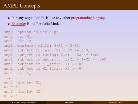
AMPL Concepts

In many ways, AMPL is like any other programming language.

Example: Bond Portfolio Model

ampl: option solver clp;ampl: var X1;ampl: var X2;ampl: maximize yield: 4*X1 + 3*X2;ampl: subject to cash: X1 + X2 <= 100;ampl: subject to rating: 2*X1 + X2 <= 150;ampl: subject to maturity: 3*X1 + 4*X2 <= 360;ampl: subject to X1_limit: X1 >= 0;ampl: subject to X2_limit: X2 >= 0;ampl: solve;...ampl: display X1;X1 = 50ampl: display X2;X2 = 50


Storing Commands in a File (bonds_simple.run)

You can type the commands into a file and then load them.

This makes it easy to modify your model later.

Example:ampl: option solver clp;ampl: model bonds_simple.mod;ampl: solve;...ampl: display X1;X1 = 50ampl: display X2;X2 = 50


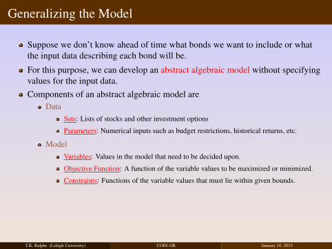
Generalizing the Model

Suppose we don’t know ahead of time what bonds we want to include or whatthe input data describing each bond will be.

For this purpose, we can develop an abstract algebraic model without specifyingvalues for the input data.Components of an abstract algebraic model are

DataSets: Lists of stocks and other investment options

Parameters: Numerical inputs such as budget restrictions, historical returns, etc.

ModelVariables: Values in the model that need to be decided upon.

Objective Function: A function of the variable values to be maximized or minimized.

Constraints: Functions of the variable values that must lie within given bounds.


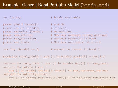
Example: General Bond Portfolio Model (bonds.mod)

set bonds; # bonds available

param yield {bonds}; # yieldsparam rating {bonds}; # ratingsparam maturity {bonds}; # maturitiesparam max_rating; # Maximum average rating allowedparam max_maturity; # Maximum maturity allowedparam max_cash; # Maximum available to invest

var buy {bonds} >= 0; # amount to invest in bond i

maximize total_yield : sum {i in bonds} yield[i] * buy[i];

subject to cash_limit : sum {i in bonds} buy[i] <= max_cash;subject to rating_limit :

sum {i in bonds} rating[i]*buy[i] <= max_cash*max_rating;subject to maturity_limit :

sum {i in bonds} maturity[i]*buy[i] <= max_cash*max_maturity;


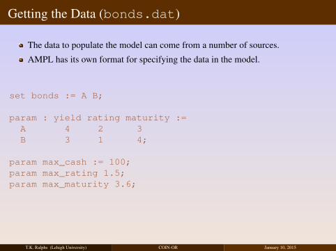
Getting the Data (bonds.dat)

The data to populate the model can come from a number of sources.

AMPL has its own format for specifying the data in the model.

set bonds := A B;

param : yield rating maturity :=A 4 2 3B 3 1 4;

param max_cash := 100;param max_rating 1.5;param max_maturity 3.6;


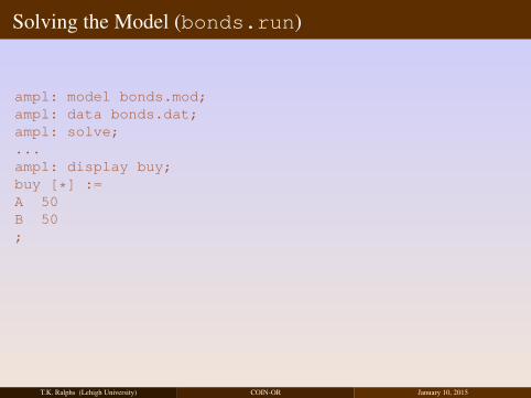
Solving the Model (bonds.run)

ampl: model bonds.mod;ampl: data bonds.dat;ampl: solve;...ampl: display buy;buy [*] :=A 50B 50;


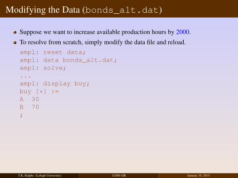
Modifying the Data (bonds_alt.dat)

Suppose we want to increase available production hours by 2000.

To resolve from scratch, simply modify the data file and reload.ampl: reset data;ampl: data bonds_alt.dat;ampl: solve;...ampl: display buy;buy [*] :=A 30B 70;


Modifying Individual Data Elements

Instead of resetting all the data, you can modify one element.ampl: reset data max_cash;ampl: data;ampl data: param max_cash := 150;ampl data: solve;...ampl: display buy;buy [*] :=A 45B 105;


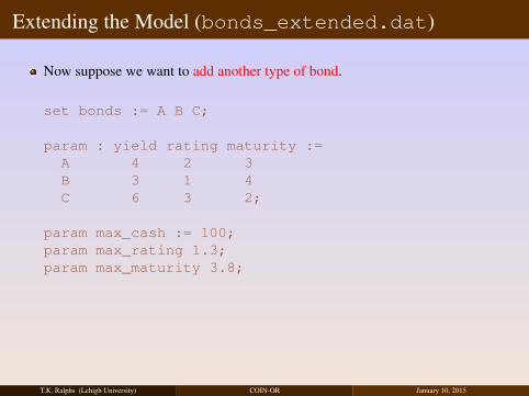
Extending the Model (bonds_extended.dat)

Now suppose we want to add another type of bond.

set bonds := A B C;

param : yield rating maturity :=A 4 2 3B 3 1 4C 6 3 2;

param max_cash := 100;param max_rating 1.3;param max_maturity 3.8;


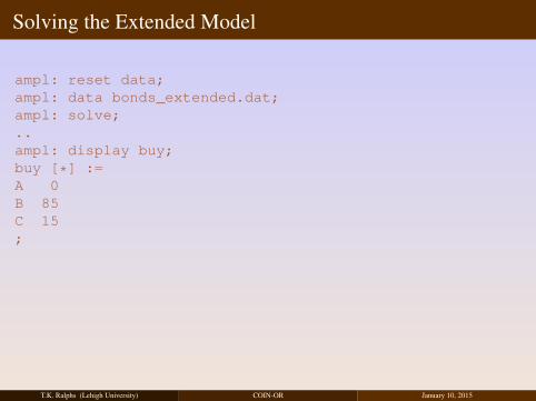
Solving the Extended Model

ampl: reset data;ampl: data bonds_extended.dat;ampl: solve;..ampl: display buy;buy [*] :=A 0B 85C 15;


Getting Data from a Spreadsheet(FinancialModels.xlsx:Bonds1-AMPL)

Another obvious source of data is a spreadsheet, such as Excel.

AMPL has commands for accessing data from a spreadsheet directly from thelanguage.

An alternative is to use SolverStudio.

SolverStudio allows the model to be composed within Excel and imports the datafrom an associated sheet.

Results can be printed to a window or output to the sheet for further analysis.


Further Generalization(FinancialModels.xlsx:Bonds2-AMPL)

Note that in our AMPL model, we essentially had three “features” of a bond thatwe wanted to take into account.

Maturity

Rating

Yield

We constrained the level of two of these and then optimized the third one.

The constraints for the features all have the same basic form.

What if we wanted to add another feature?

We can make the list of features a set and use the concept of a two-dimensionalparameter to create a table of bond data.


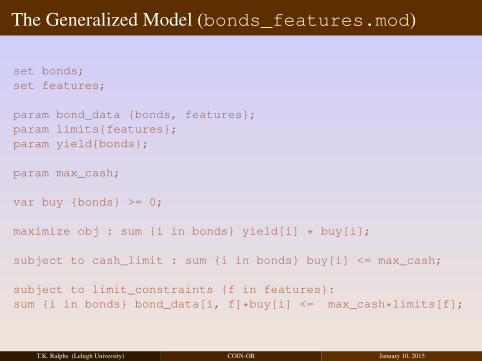
The Generalized Model (bonds_features.mod)

set bonds;set features;

param bond_data {bonds, features};param limits{features};param yield{bonds};

param max_cash;

var buy {bonds} >= 0;

maximize obj : sum {i in bonds} yield[i] * buy[i];

subject to cash_limit : sum {i in bonds} buy[i] <= max_cash;

subject to limit_constraints {f in features}:sum {i in bonds} bond_data[i, f]*buy[i] <= max_cash*limits[f];


Outline

1 Introduction

2 Solver Studio





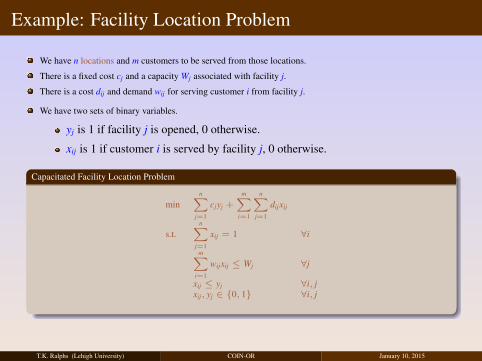
Example: Facility Location Problem

We have n locations and m customers to be served from those locations.

There is a fixed cost cj and a capacity Wj associated with facility j.

There is a cost dij and demand wij for serving customer i from facility j.

We have two sets of binary variables.

yj is 1 if facility j is opened, 0 otherwise.

xij is 1 if customer i is served by facility j, 0 otherwise.

Capacitated Facility Location Problem

minn∑

j=1

cjyj +

m∑i=1

n∑j=1

dijxij

s.t.n∑

j=1

xij = 1 ∀i

m∑i=1

wijxij ≤ Wj ∀j

xij ≤ yj ∀i, jxij, yj ∈ {0, 1} ∀i, j


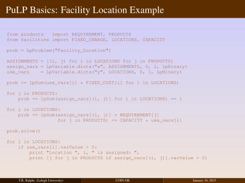
PuLP Basics: Facility Location Example

from products import REQUIREMENT, PRODUCTSfrom facilities import FIXED_CHARGE, LOCATIONS, CAPACITY

prob = LpProblem("Facility_Location")

ASSIGNMENTS = [(i, j) for i in LOCATIONS for j in PRODUCTS]assign_vars = LpVariable.dicts("x", ASSIGNMENTS, 0, 1, LpBinary)use_vars = LpVariable.dicts("y", LOCATIONS, 0, 1, LpBinary)

prob += lpSum(use_vars[i] * FIXED_COST[i] for i in LOCATIONS)

for j in PRODUCTS:prob += lpSum(assign_vars[(i, j)] for i in LOCATIONS) == 1

for i in LOCATIONS:prob += lpSum(assign_vars[(i, j)] * REQUIREMENT[j]

for j in PRODUCTS) <= CAPACITY * use_vars[i]

prob.solve()

for i in LOCATIONS:if use_vars[i].varValue > 0:

print "Location ", i, " is assigned: ",print [j for j in PRODUCTS if assign_vars[(i, j)].varValue > 0]


PuLP Basics: Facility Location Example

# The requirements for the productsREQUIREMENT = {

1 : 7,2 : 5,3 : 3,4 : 2,5 : 2,

}# Set of all productsPRODUCTS = REQUIREMENT.keys()PRODUCTS.sort()# Costs of the facilitiesFIXED_COST = {

1 : 10,2 : 20,3 : 16,4 : 1,5 : 2,

}# Set of facilitiesLOCATIONS = FIXED_COST.keys()LOCATIONS.sort()# The capacity of the facilitiesCAPACITY = 8


Dippy Basics

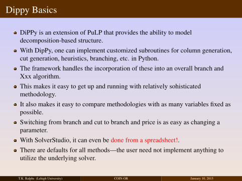
DiPPy is an extension of PuLP that provides the ability to modeldecomposition-based structure.With DipPy, one can implement customized subroutines for column generation,cut generation, heuristics, branching, etc. in Python.The framework handles the incorporation of these into an overall branch andXxx algorithm.This makes it easy to get up and running with relatively sohisticatedmethodology.It also makes it easy to compare methodologies with as many variables fixed aspossible.Switching from branch and cut to branch and price is as easy as changing aparameter.With SolverStudio, it can even be done from a spreadsheet!.There are defaults for all methods—the user need not implement anything toutilize the underlying solver.


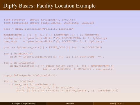
DipPy Basics: Facility Location Example

from products import REQUIREMENT, PRODUCTSfrom facilities import FIXED_CHARGE, LOCATIONS, CAPACITY

prob = dippy.DipProblem("Facility_Location")

ASSIGNMENTS = [(i, j) for i in LOCATIONS for j in PRODUCTS]assign_vars = LpVariable.dicts("x", ASSIGNMENTS, 0, 1, LpBinary)use_vars = LpVariable.dicts("y", LOCATIONS, 0, 1, LpBinary)

prob += lpSum(use_vars[i] * FIXED_COST[i] for i in LOCATIONS)

for j in PRODUCTS:prob += lpSum(assign_vars[(i, j)] for i in LOCATIONS) == 1

for i in LOCATIONS:prob.relaxation[i] += lpSum(assign_vars[(i, j)] * REQUIREMENT[j]

for j in PRODUCTS) <= CAPACITY * use_vars[i]

dippy.Solve(prob, {doPriceCut:1})

for i in LOCATIONS:if use_vars[i].varValue > 0:

print "Location ", i, " is assigned: ",print [j for j in PRODUCTS if assign_vars[(i, j)].varValue > 0]


«««< Updated upstream


Dippy Callbacks

def solve_subproblem(prob, index, redCosts, convexDual):...return knapsack01(obj, weights, CAPACITY)

def knapsack01(obj, weights, capacity):...return solution

def first_fit(prob):...return bvs

prob.init_vars = first_fitdef choose_branch(prob, sol):

...return ([], down_branch_ub, up_branch_lb, [])

def generate_cuts(prob, sol):...return new_cuts

def heuristics(prob, xhat, cost):...return sols

dippy.Solve(prob, {’doPriceCut’: ’1’})T.K. Ralphs (Lehigh University) COIN-OR January 10, 2015

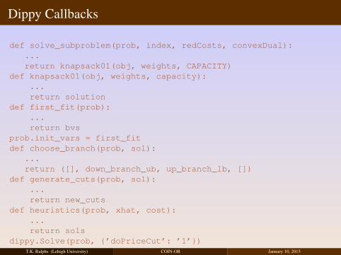
Dippy Callbacks

def solve_subproblem(prob, index, redCosts, convexDual):...return knapsack01(obj, weights, CAPACITY)

def knapsack01(obj, weights, capacity):...return solution

def first_fit(prob):...return bvs

prob.init_vars = first_fitdef choose_branch(prob, sol):

...return ([], down_branch_ub, up_branch_lb, [])

def generate_cuts(prob, sol):...return new_cuts

def heuristics(prob, xhat, cost):...return sols

dippy.Solve(prob, {’doPriceCut’: ’1’})T.K. Ralphs (Lehigh University) COIN-OR January 10, 2015

Pyomo Basics

In contrast to PuLP, Pyomo allows the creaton of “abstract” models, like otherAMLs.Note, however, that it can also be used to create concrete models, like PuLP.Like, it can read data from a wide range of source.It also allows constraints to involve more general functions.As we will see, this power comes with some increased complexity.


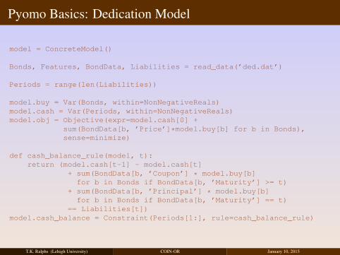
Pyomo Basics: Dedication Model

model = ConcreteModel()

Bonds, Features, BondData, Liabilities = read_data(’ded.dat’)

Periods = range(len(Liabilities))

model.buy = Var(Bonds, within=NonNegativeReals)model.cash = Var(Periods, within=NonNegativeReals)model.obj = Objective(expr=model.cash[0] +

sum(BondData[b, ’Price’]*model.buy[b] for b in Bonds),sense=minimize)

def cash_balance_rule(model, t):return (model.cash[t-1] - model.cash[t]

+ sum(BondData[b, ’Coupon’] * model.buy[b]for b in Bonds if BondData[b, ’Maturity’] >= t)

+ sum(BondData[b, ’Principal’] * model.buy[b]for b in Bonds if BondData[b, ’Maturity’] == t)

== Liabilities[t])model.cash_balance = Constraint(Periods[1:], rule=cash_balance_rule)


Outline

1 Introduction

2 Solver Studio





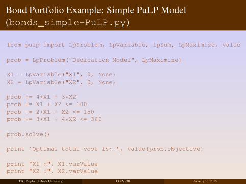
Bond Portfolio Example: Simple PuLP Model(bonds_simple-PuLP.py)

from pulp import LpProblem, LpVariable, lpSum, LpMaximize, value

prob = LpProblem("Dedication Model", LpMaximize)

X1 = LpVariable("X1", 0, None)X2 = LpVariable("X2", 0, None)

prob += 4*X1 + 3*X2prob += X1 + X2 <= 100prob += 2*X1 + X2 <= 150prob += 3*X1 + 4*X2 <= 360

prob.solve()

print ’Optimal total cost is: ’, value(prob.objective)

print "X1 :", X1.varValueprint "X2 :", X2.varValue


Notes About the Model

Like the simple AMPL model, we are not using indexing or any sort ofabstraction here.

The syntax is very similar to AMPL.

To achieve separation of data and model, we use Python’s import mechanism.


Bond Portfolio Example: Abstract PuLP Model(bonds-PuLP.py)

from pulp import LpProblem, LpVariable, lpSum, LpMaximize, value

from bonds import bonds, max_rating, max_maturity, max_cash

prob = LpProblem("Bond Selection Model", LpMaximize)

buy = LpVariable.dicts(’bonds’, bonds.keys(), 0, None)

prob += lpSum(bonds[b][’yield’] * buy[b] for b in bonds)

prob += lpSum(buy[b] for b in bonds) <= max_cash, "cash"

prob += (lpSum(bonds[b][’rating’] * buy[b] for b in bonds)<= max_cash*max_rating, "ratings")

prob += (lpSum(bonds[b][’maturity’] * buy[b] for b in bonds)<= max_cash*max_maturity, "maturities")


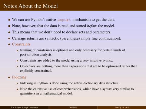
Notes About the Model

We can use Python’s native import mechanism to get the data.

Note, however, that the data is read and stored before the model.

This means that we don’t need to declare sets and parameters.

Carriage returns are syntactic (parentheses imply line continuation).Constraints

Naming of constraints is optional and only necessary for certain kinds ofpost-solution analysis.

Constraints are added to the model using a very intuitive syntax.

Objectives are nothing more than expressions that are to be optimized rather thanexplicitly constrained.

IndexingIndexing in Python is done using the native dictionary data structure.

Note the extensive use of comprehensions, which have a syntax very similar toquantifiers in a mathematical model.


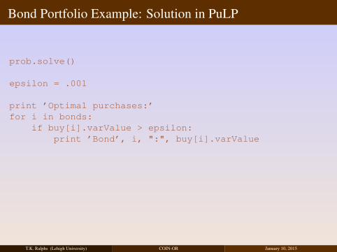
Bond Portfolio Example: Solution in PuLP

prob.solve()

epsilon = .001

print ’Optimal purchases:’for i in bonds:

if buy[i].varValue > epsilon:print ’Bond’, i, ":", buy[i].varValue


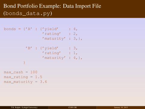
Bond Portfolio Example: Data Import File(bonds_data.py)

bonds = {’A’ : {’yield’ : 4,’rating’ : 2,’maturity’ : 3,},

’B’ : {’yield’ : 3,’rating’ : 1,’maturity’ : 4,},

}

max_cash = 100max_rating = 1.5max_maturity = 3.6


Notes About the Data Import

We are storing the data about the bonds in a “dictionary of dictionaries.”

With this data structure, we don’t need to separately construct the list of bonds.

We can access the list of bonds as bonds.keys().

Note, however, that we still end up hard-coding the list of features and we mustrepeat this list of features for every bond.

We can avoid this using some advanced Python programming techniques, butSolverStudio makes this easy.


Bond Portfolio Example: PuLP Model in SolverStudio(FinancialModels.xlsx:Bonds-PuLP)

buy = LpVariable.dicts(’bonds’, bonds, 0, None)for f in features:

if limits[f] == "Opt":if sense[f] == ’>’:

prob += lpSum(bond_data[b, f] * buy[b] for b in bonds)else:

prob += lpSum(-bond_data[b, f] * buy[b] for b in bonds)else:

if sense[f] == ’>’:prob += (lpSum(bond_data[b,f]*buy[b] for b in bonds) >=

max_cash*limits[f], f)else:

prob += (lpSum(bond_data[b,f]*buy[b] for b in bonds) <=max_cash*limits[f], f)

prob += lpSum(buy[b] for b in bonds) <= max_cash, "cash"


Notes About the SolverStudio PuLP Model

We’ve explicitly allowed the option of optimizing over one of the features, whileconstraining the others.

Later, we’ll see how to create tradeoff curves showing the tradeoffs among theconstraints imposed on various features.


Portfolio Dedication

Definition 1 Dedication or cash flow matching refers to the funding of known futureliabilities through the purchase of a portfolio of risk-free non-callable bonds.

Notes:

Dedication is used to eliminate interest rate risk.

Dedicated portfolios do not have to be managed.

The goal is to construct such portfolio at a minimal price from a set of availablebonds.

This is a multi-period model.


Example: Portfolio Dedication

A pension fund faces liabilities totalling `j for years j = 1, ...,T .

The fund wishes to dedicate these liabilities via a portfolio comprised of ndifferent types of bonds.

Bond type i costs ci, matures in year mi, and yields a yearly coupon payment ofdi up to maturity.

The principal paid out at maturity for bond i is pi.


LP Formulation for Portfolio Dedication

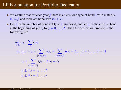
We assume that for each year j there is at least one type of bond i with maturitymi = j, and there are none with mi > T .

Let xi be the number of bonds of type i purchased, and let zj be the cash on handat the beginning of year j for j = 0, . . . ,T . Then the dedication problem is thefollowing LP.

min(x,z)

z0 +∑

i

cixi

s.t. zj−1 − zj +∑{i:mi≥j}

dixi +∑{i:mi=j}

pixi = `j, (j = 1, . . . ,T − 1)

zT +∑{i:mi=T}

(pi + di)xi = `T .

zj ≥ 0, j = 1, . . . ,T

xi ≥ 0, i = 1, . . . , n


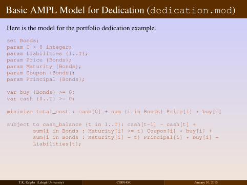
Basic AMPL Model for Dedication (dedication.mod)

Here is the model for the portfolio dedication example.

set Bonds;param T > 0 integer;param Liabilities {1..T};param Price {Bonds};param Maturity {Bonds};param Coupon {Bonds};param Principal {Bonds};

var buy {Bonds} >= 0;var cash {0..T} >= 0;

minimize total_cost : cash[0] + sum {i in Bonds} Price[i] * buy[i]

subject to cash_balance {t in 1..T}: cash[t-1] - cash[t] +sum{i in Bonds : Maturity[i] >= t} Coupon[i] * buy[i] +sum{i in Bonds : Maturity[i] = t} Principal[i] * buy[i] =Liabilities[t];


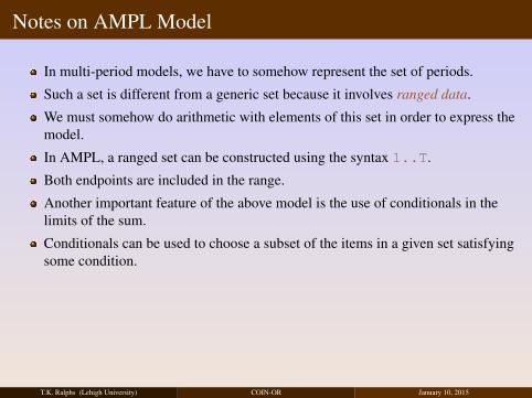
Notes on AMPL Model

In multi-period models, we have to somehow represent the set of periods.

Such a set is different from a generic set because it involves ranged data.

We must somehow do arithmetic with elements of this set in order to express themodel.

In AMPL, a ranged set can be constructed using the syntax 1..T.

Both endpoints are included in the range.

Another important feature of the above model is the use of conditionals in thelimits of the sum.

Conditionals can be used to choose a subset of the items in a given set satisfyingsome condition.


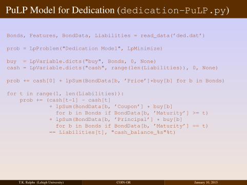
PuLP Model for Dedication (dedication-PuLP.py)


prob = LpProblem("Dedication Model", LpMinimize)

buy = LpVariable.dicts("buy", Bonds, 0, None)cash = LpVariable.dicts("cash", range(len(Liabilities)), 0, None)

prob += cash[0] + lpSum(BondData[b, ’Price’]*buy[b] for b in Bonds)

for t in range(1, len(Liabilities)):prob += (cash[t-1] - cash[t]

+ lpSum(BondData[b, ’Coupon’] * buy[b]for b in Bonds if BondData[b, ’Maturity’] >= t)

+ lpSum(BondData[b, ’Principal’] * buy[b]for b in Bonds if BondData[b, ’Maturity’] == t)

== Liabilities[t], "cash_balance_%s"%t)


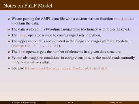
Notes on PuLP Model

We are parsing the AMPL data file with a custom-written function read_datato obtain the data.

The data is stored in a two-dimensional table (dictionary with tuples as keys).

The range operator is used to create ranged sets in Python.

The upper endpoint is not included in the range and ranges start at 0 by default(range(3) = [0, 1, 2]).

The len operator gets the number of elements in a given data structure.

Python also supports conditions in comprehensions, so the model reads naturallyin Python’s native syntax.

See also FinancialModels.xlsx:Dedication-PuLP.


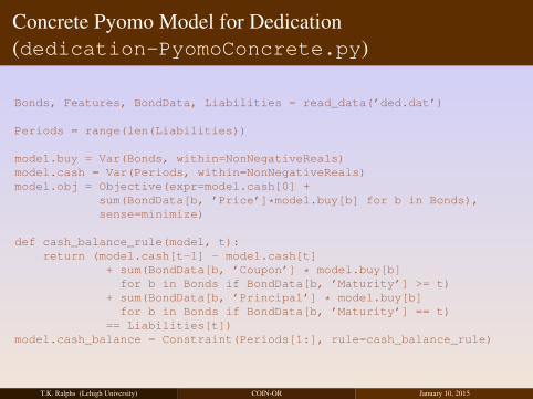
Concrete Pyomo Model for Dedication(dedication-PyomoConcrete.py)


Periods = range(len(Liabilities))

model.buy = Var(Bonds, within=NonNegativeReals)model.cash = Var(Periods, within=NonNegativeReals)model.obj = Objective(expr=model.cash[0] +

sum(BondData[b, ’Price’]*model.buy[b] for b in Bonds),sense=minimize)


+ sum(BondData[b, ’Coupon’] * model.buy[b]for b in Bonds if BondData[b, ’Maturity’] >= t)

+ sum(BondData[b, ’Principal’] * model.buy[b]for b in Bonds if BondData[b, ’Maturity’] == t)

== Liabilities[t])model.cash_balance = Constraint(Periods[1:], rule=cash_balance_rule)


Notes on the Concrete Pyomo Model

This model is almost identical to the PuLP model.

The only substantial difference is the way in which constraints are defined, using“rules.”

Indexing is implemented by specifying additional arguments to the rulefunctions.

When the rule function specifies an indexed set of constraints, the indices arepassed through the arguments to the function.

The model is constructed by looping over the index set, constructing eachassociated constraint.

Note the use of the Python slice operator to extract a subset of a ranged set.


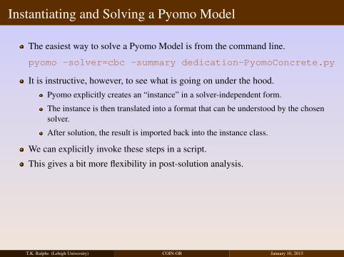
Instantiating and Solving a Pyomo Model

The easiest way to solve a Pyomo Model is from the command line.

pyomo -solver=cbc -summary dedication-PyomoConcrete.py

It is instructive, however, to see what is going on under the hood.Pyomo explicitly creates an “instance” in a solver-independent form.

The instance is then translated into a format that can be understood by the chosensolver.

After solution, the result is imported back into the instance class.

We can explicitly invoke these steps in a script.

This gives a bit more flexibility in post-solution analysis.


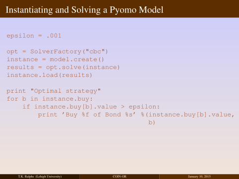
Instantiating and Solving a Pyomo Model

epsilon = .001

opt = SolverFactory("cbc")instance = model.create()results = opt.solve(instance)instance.load(results)

print "Optimal strategy"for b in instance.buy:

if instance.buy[b].value > epsilon:print ’Buy %f of Bond %s’ %(instance.buy[b].value,

b)


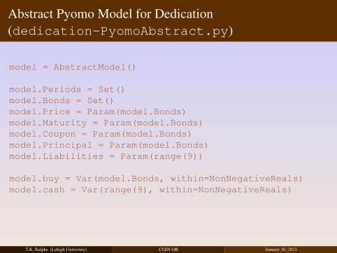
Abstract Pyomo Model for Dedication(dedication-PyomoAbstract.py)

model = AbstractModel()

model.Periods = Set()model.Bonds = Set()model.Price = Param(model.Bonds)model.Maturity = Param(model.Bonds)model.Coupon = Param(model.Bonds)model.Principal = Param(model.Bonds)model.Liabilities = Param(range(9))

model.buy = Var(model.Bonds, within=NonNegativeReals)model.cash = Var(range(9), within=NonNegativeReals)


Abstract Pyomo Model for Dedication (cont’d)

def objective_rule(model):return model.cash[0] + sum(model.Price[b]*model.buy[b]

for b in model.Bonds)model.objective = Objective(sense=minimize, rulre=objective_rule)


+ sum(model.Coupon[b] * model.buy[b]for b in model.Bonds if model.Maturity[b] >= t)

+ sum(model.Principal[b] * model.buy[b]for b in model.Bonds if model.Maturity[b] == t)

== model.Liabilities[t])

model.cash_balance = Constraint(range(1, 9), rue=cash_balance_rule)


Notes on the Abstract Pyomo Model

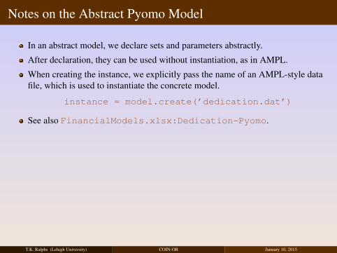
In an abstract model, we declare sets and parameters abstractly.

After declaration, they can be used without instantiation, as in AMPL.

When creating the instance, we explicitly pass the name of an AMPL-style datafile, which is used to instantiate the concrete model.

instance = model.create(’dedication.dat’)

See also FinancialModels.xlsx:Dedication-Pyomo.


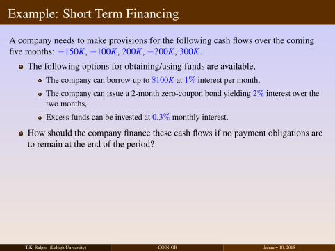
Example: Short Term Financing

A company needs to make provisions for the following cash flows over the comingfive months: −150K, −100K, 200K, −200K, 300K.

The following options for obtaining/using funds are available,The company can borrow up to $100K at 1% interest per month,

The company can issue a 2-month zero-coupon bond yielding 2% interest over thetwo months,

Excess funds can be invested at 0.3% monthly interest.

How should the company finance these cash flows if no payment obligations areto remain at the end of the period?


Example (cont.)

All investments are risk-free, so there is no stochasticity.What are the decision variables?

xi, the amount drawn from the line of credit in month i,

yi, the number of bonds issued in month i,

zi, the amount invested in month i,

What is the goal?To maximize the cash on hand at the end of the horizon.


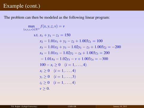
Example (cont.)

The problem can then be modeled as the following linear program:

max(x,y,z,v)∈R12

f (x, y, z, v) = v

s.t. x1 + y1 − z1 = 150x2 − 1.01x1 + y2 − z2 + 1.003z1 = 100x3 − 1.01x2 + y3 − 1.02y1 − z3 + 1.003z2 = −200x4 − 1.01x3 − 1.02y2 − z4 + 1.003z3 = 200− 1.01x4 − 1.02y3 − v + 1.003z4 = −300100 − xi ≥ 0 (i = 1, . . . , 4)xi ≥ 0 (i = 1, . . . , 4)yi ≥ 0 (i = 1, . . . , 3)zi ≥ 0 (i = 1, . . . , 4)v ≥ 0.


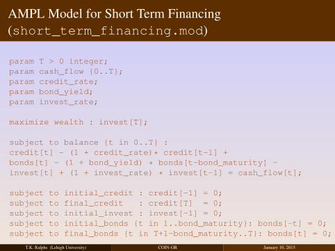
AMPL Model for Short Term Financing(short_term_financing.mod)

param T > 0 integer;param cash_flow {0..T};param credit_rate;param bond_yield;param invest_rate;

maximize wealth : invest[T];

subject to balance {t in 0..T} :credit[t] - (1 + credit_rate)* credit[t-1] +bonds[t] - (1 + bond_yield) * bonds[t-bond_maturity] -invest[t] + (1 + invest_rate) * invest[t-1] = cash_flow[t];

subject to initial_credit : credit[-1] = 0;subject to final_credit : credit[T] = 0;subject to initial_invest : invest[-1] = 0;subject to initial_bonds {t in 1..bond_maturity}: bonds[-t] = 0;subject to final_bonds {t in T+1-bond_maturity..T}: bonds[t] = 0;


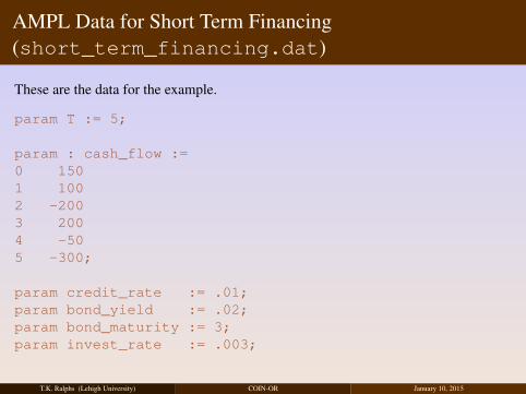
AMPL Data for Short Term Financing(short_term_financing.dat)

These are the data for the example.

param T := 5;

param : cash_flow :=0 1501 1002 -2003 2004 -505 -300;

param credit_rate := .01;param bond_yield := .02;param bond_maturity := 3;param invest_rate := .003;


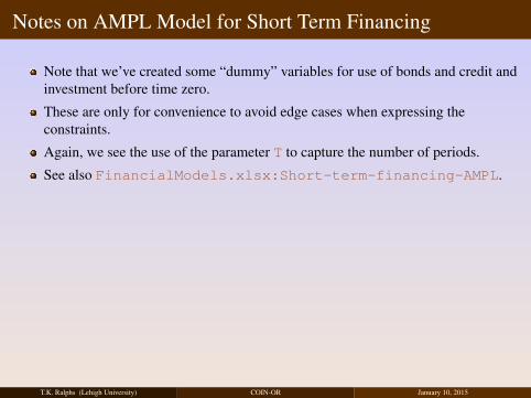
Notes on AMPL Model for Short Term Financing

Note that we’ve created some “dummy” variables for use of bonds and credit andinvestment before time zero.

These are only for convenience to avoid edge cases when expressing theconstraints.

Again, we see the use of the parameter T to capture the number of periods.

See also FinancialModels.xlsx:Short-term-financing-AMPL.


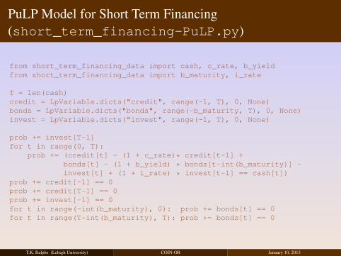
PuLP Model for Short Term Financing(short_term_financing-PuLP.py)

from short_term_financing_data import cash, c_rate, b_yieldfrom short_term_financing_data import b_maturity, i_rate

T = len(cash)credit = LpVariable.dicts("credit", range(-1, T), 0, None)bonds = LpVariable.dicts("bonds", range(-b_maturity, T), 0, None)invest = LpVariable.dicts("invest", range(-1, T), 0, None)

prob += invest[T-1]for t in range(0, T):

prob += (credit[t] - (1 + c_rate)* credit[t-1] +bonds[t] - (1 + b_yield) * bonds[t-int(b_maturity)] -invest[t] + (1 + i_rate) * invest[t-1] == cash[t])

prob += credit[-1] == 0prob += credit[T-1] == 0prob += invest[-1] == 0for t in range(-int(b_maturity), 0): prob += bonds[t] == 0for t in range(T-int(b_maturity), T): prob += bonds[t] == 0


Documents

Introduction to the COIN-OR Optimization Suitecoral.ie.lehigh.edu/~ted/files/coin-or/slides/COINModeling.pdf · The COIN-OR Optimization Suite: Open Source Tools for Optimization