Embed Size (px)
Citation preview

Overview of ProbabilityStochastic AnalysisMajor Applications
Conclusion
Introduction to Stochastic Analysis
Christopher W. Miller
Department of MathematicsUniversity of California, Berkeley
February 12, 2014
C. Miller Stochastic Analysis

Overview of ProbabilityStochastic AnalysisMajor Applications
Conclusion
Background and Motivation
Consider the ordinary differential equation:X ′(t) = µ (X (t), t)
X (0) = x0,
which defines a trajectory x : [0,∞)→ Rn.
C. Miller Stochastic Analysis

Overview of ProbabilityStochastic AnalysisMajor Applications
Conclusion
Background and Motivation
In practice, solutions often display noise. We may want to model inthe form:
dX
dt= µ (X (t), t) + σ (X (t), t) · ηt ,
with ηt satisfying, at least approximately,
ηt1 and ηt2 are independent when t1 6= t2,
ηt is stationary, i.e. distribution is translation invariant,
E [ηt ] = 0 for all t.
It turns out no reasonable stochastic process exists satisfying these.
C. Miller Stochastic Analysis

Overview of ProbabilityStochastic AnalysisMajor Applications
Conclusion
Background and Motivation
In practice, solutions often display noise. We may want to model inthe form:
dX
dt= µ (X (t), t) + σ (X (t), t) · ηt ,
with ηt satisfying, at least approximately,
ηt1 and ηt2 are independent when t1 6= t2,
ηt is stationary, i.e. distribution is translation invariant,
E [ηt ] = 0 for all t.
It turns out no reasonable stochastic process exists satisfying these.C. Miller Stochastic Analysis

Overview of ProbabilityStochastic AnalysisMajor Applications
Conclusion
Background and Motivation
Re-interpret as an integral equation:
X (t) = X (0) +
∫ t
0µ (X (s), s) ds +
∫ t
0σ (X (s), s) dWs .
Goals of this talk:
Motivate a definition of the stochastic integral,
Explore the properties of Brownian motion,
Highlight major applications of stochastic analysis to PDEand control theory.
References:
”An Intro. to Stochastic Differential Equations”, L.C. Evans
”Brownian Motion and Stoch. Calculus”, Karatzas and Shreve
C. Miller Stochastic Analysis

Overview of ProbabilityStochastic AnalysisMajor Applications
Conclusion
Background and Motivation
Re-interpret as an integral equation:
X (t) = X (0) +
∫ t
0µ (X (s), s) ds +
∫ t
0σ (X (s), s) dWs .
Goals of this talk:
Motivate a definition of the stochastic integral,
Explore the properties of Brownian motion,
Highlight major applications of stochastic analysis to PDEand control theory.
References:
”An Intro. to Stochastic Differential Equations”, L.C. Evans
”Brownian Motion and Stoch. Calculus”, Karatzas and Shreve
C. Miller Stochastic Analysis

Overview of ProbabilityStochastic AnalysisMajor Applications
Conclusion
Table of contents
1 Overview of ProbabilityProbability SpacesRandom VariablesStochastic Processes
2 Stochastic AnalysisBrownian MotionStochastic IntegrationIto’s Formula
3 Major ApplicationsMartingale Representation TheoremFeynman-Kac FormulaHamilton-Jacobi-Bellman Equation
C. Miller Stochastic Analysis

Overview of ProbabilityStochastic AnalysisMajor Applications
Conclusion
Probability SpacesRandom VariablesStochastic Processes
Probability Spaces
We want to define a probability space (Ω,F ,P) to capture theformal notions:
Ω is a set of ”outcomes”
F is a collection of ”events”
P measures the likelihood of different ”events”.
Definition (σ-algebra)
If Ω is a given set, then a σ-algebra F on Ω is a collection F ofsubsets on Ω with the following properties:
1 ∅ ∈ F2 A ∈ F =⇒ Ac ∈ F3 A1,A2, . . . ∈ F =⇒
⋃∞i=1 Ai ∈ F .
C. Miller Stochastic Analysis

Overview of ProbabilityStochastic AnalysisMajor Applications
Conclusion
Probability SpacesRandom VariablesStochastic Processes
Probability Spaces
Definition (Probability measure)
Given a pair (Ω,F), then a probability measure P is a functionP : F → [0, 1] such that:
1 P (∅) = 0, P (Ω) = 1
2 If A1,A2, . . . ∈ F are pairwise disjoint, then
P (∪∞i=1Ai ) =∞∑i=1
P (Ai ) .
We call a triple (Ω,F ,P) a probability space.
C. Miller Stochastic Analysis

Overview of ProbabilityStochastic AnalysisMajor Applications
Conclusion
Probability SpacesRandom VariablesStochastic Processes
Random Variables
Definition (Random variable)
Let (Ω,F ,P) be a probability space. A function X : Ω→ Rn iscalled a random variable if for each B ∈ B, we have
X−1(B) ∈ F .
Equivalently, we say X is F-measurable.
Proposition
Let X : Ω→ Rn be a random variable. Then
σ(X ) = X−1(B)|B ∈ B
is a σ-algebra, called the σ-algebra generated by X .
C. Miller Stochastic Analysis

Overview of ProbabilityStochastic AnalysisMajor Applications
Conclusion
Probability SpacesRandom VariablesStochastic Processes
Random Variables
Proposition
Let X : Ω→ Rn be a random variable on a probability space(Ω,F ,P). Then
µX (B) = P[X−1(B)
]for each B ∈ B is a measure on Rn called the distribution of X .
Definition (Expectation)
Let X : Ω→ Rn be a random variable and f : Rn → R be Borelmeasurable. Then the expectation of f (X ) may be defined as:
E [f (X )] =
∫Rn
f (x) dµX (x).
C. Miller Stochastic Analysis

Overview of ProbabilityStochastic AnalysisMajor Applications
Conclusion
Probability SpacesRandom VariablesStochastic Processes
Random Variables
Definition (Conditional Expectation)
Let X be F-measurable and G ⊂ F be a sub-σ-algebra. Then aconditional expectation of X given G is any G-measurable functionE [X |G] such that
E [E [X |G] 1A] = E [X 1A]
for any A ∈ G.
Proposition (Some Properties of Conditional Expectation)
Linearity in E [· | G].
If X is G-measurable, then E [XY | G] = X E [Y | G] a.s. aslong as XY is integrable.
If H ⊂ G, then E [X | H] = E [E [X | G] | H] a.s.
C. Miller Stochastic Analysis

Overview of ProbabilityStochastic AnalysisMajor Applications
Conclusion
Probability SpacesRandom VariablesStochastic Processes
Random Variables
Definition (Conditional Expectation)
Let X be F-measurable and G ⊂ F be a sub-σ-algebra. Then aconditional expectation of X given G is any G-measurable functionE [X |G] such that
E [E [X |G] 1A] = E [X 1A]
for any A ∈ G.
Proposition (Some Properties of Conditional Expectation)
Linearity in E [· | G].
If X is G-measurable, then E [XY | G] = X E [Y | G] a.s. aslong as XY is integrable.
If H ⊂ G, then E [X | H] = E [E [X | G] | H] a.s.C. Miller Stochastic Analysis

Overview of ProbabilityStochastic AnalysisMajor Applications
Conclusion
Probability SpacesRandom VariablesStochastic Processes
Stochastic Processes
Definition (Stochastic process)
A collection Xt : t ∈ T of random variables is called astochastic process.
For each ω ∈ Ω, the mapping t 7→ X (t, ω) is thecorresponding sample path.
Examples:
Simple random walk
Markov chain
· · ·
C. Miller Stochastic Analysis

Overview of ProbabilityStochastic AnalysisMajor Applications
Conclusion
Probability SpacesRandom VariablesStochastic Processes
Stochastic Processes
Proposition
Let Xn be a stochastic process. The sequence of σ-algebrasdefined by:
Fn = σ (X0,X1, . . . ,Xn) .
is an increasing sequence. We call such an increasing sequence ofσ-algebras a filtration.
Definition (Martingale)
Let Xn be a stochastic process such that each Xn isFn-measurable. We say Xn is a martingale if
Xn ∈ L1(Ω,F ,P) for all n ≥ 0
E [Xn+1|Fn] = Xn for all n ≥ 0.
C. Miller Stochastic Analysis

Overview of ProbabilityStochastic AnalysisMajor Applications
Conclusion
Probability SpacesRandom VariablesStochastic Processes
Stochastic Processes
Proposition
The simple random walk is a martingale if and only if p = 12 .
Proof.
Recall, a simple random walk is Xn =∑n
k=1 ξk , where ξnn≥0 areIID with P [ξn = 1] = 1− P [ξ = −1] = p ∈ (0, 1).
E [|Xn|] ≤n∑
k=1
E [|ξk |] = n
E [Xn+1|Fn] = E [Xn + ξn+1|Fn]
= Xn + E [ξn+1|Fn] = Xn + 2p − 1.
C. Miller Stochastic Analysis
Overview of ProbabilityStochastic AnalysisMajor Applications
Conclusion
Probability SpacesRandom VariablesStochastic Processes
Stochastic Processes
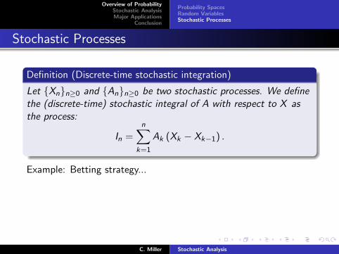
Definition (Discrete-time stochastic integration)
Let Xnn≥0 and Ann≥0 be two stochastic processes. We definethe (discrete-time) stochastic integral of A with respect to X asthe process:
In =n∑
k=1
Ak (Xk − Xk−1) .
Example: Betting strategy...
Proposition
If Xn is a martingale and An is a ”predictable”, L∞(Ω)process, then In is a martingale.
C. Miller Stochastic Analysis

Overview of ProbabilityStochastic AnalysisMajor Applications
Conclusion
Probability SpacesRandom VariablesStochastic Processes
Stochastic Processes
Proposition
If Xn is a martingale and An is a predictable, L∞(Ω) process,then In is a martingale.
Proof.
Note, each In is Fn-measurable. Holder’s inequality showsIn ∈ L1(Ω). We check the last condition using predictability of A:
E [In+1|Fn] = E [In + An+1 (Xn+1 − Xn) |Fn]
= In + An+1E [Xn+1 − Xn|Fn] = In.
Interpretation: Impossible to make money betting on a martingale.
C. Miller Stochastic Analysis

Overview of ProbabilityStochastic AnalysisMajor Applications
Conclusion
Brownian MotionStochastic IntegrationIto’s Formula
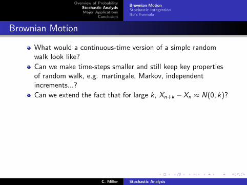
Brownian Motion
What would a continuous-time version of a simple randomwalk look like?
Can we make time-steps smaller and still keep key propertiesof random walk, e.g. martingale, Markov, independentincrements...?
Can we extend the fact that for large k , Xn+k −Xn ≈ N(0, k)?
Definition (Brownian Motion)
A real-valued stochastic process W is called a Brownian motion if:
1 W0 = 0 almost surely,
2 Wt −Ws is N(0, t − s) for all t ≥ s ≥ 0,
3 for all times 0 < t1 < t2 < · · · < tn, the random variablesWt1 , Wt2 −Wt1 , . . ., Wtn −Wtn−1 are independent.
C. Miller Stochastic Analysis

Overview of ProbabilityStochastic AnalysisMajor Applications
Conclusion
Brownian MotionStochastic IntegrationIto’s Formula
Brownian Motion
What would a continuous-time version of a simple randomwalk look like?
Can we make time-steps smaller and still keep key propertiesof random walk, e.g. martingale, Markov, independentincrements...?
Can we extend the fact that for large k , Xn+k −Xn ≈ N(0, k)?
Definition (Brownian Motion)
A real-valued stochastic process W is called a Brownian motion if:
1 W0 = 0 almost surely,
2 Wt −Ws is N(0, t − s) for all t ≥ s ≥ 0,
3 for all times 0 < t1 < t2 < · · · < tn, the random variablesWt1 , Wt2 −Wt1 , . . ., Wtn −Wtn−1 are independent.
C. Miller Stochastic Analysis

Overview of ProbabilityStochastic AnalysisMajor Applications
Conclusion
Brownian MotionStochastic IntegrationIto’s Formula
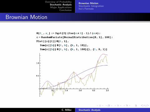
Brownian Motion
Theorem (Sketch of Existence)
Let wk be an orthonormal basis on L2(0, 1). Let ξk be asequence of independent, N(0, 1) random variables. The sum
Wt(ω) =∞∑k=0
ξk(ω)
∫ t
0wk(s) ds
converges uniformly in t almost surely. Wt is a Brownian motionfor 0 ≤ t ≤ 1, and furthermore, t 7→Wt(ω) is continuous almostsurely.
Proof
We ignore all technical issues of convergence and just check thejoint distributions of increments.
C. Miller Stochastic Analysis

Overview of ProbabilityStochastic AnalysisMajor Applications
Conclusion
Brownian MotionStochastic IntegrationIto’s Formula
Brownian Motion
A sum of normal random variables is normal.
E[Wtm+1 −Wtm
]=∞∑k=1
∫ tm+1
tm
wk ds E [ξk ] = 0.
E [∆Wtm ∆Wtn ] =∑k,l
∫ tm+1
tm
wk ds
∫ tn+1
tn
wl dsE [ξkξl ]
=∞∑k=0
∫ tm+1
tm
wk ds
∫ tn+1
tn
wk ds
=
∫ 1
01[tm,tm+1] 1[tn,tn+1] ds = ∆tm δ
mn .
C. Miller Stochastic Analysis
Overview of ProbabilityStochastic AnalysisMajor Applications
Conclusion
Brownian MotionStochastic IntegrationIto’s Formula
Brownian Motion
C. Miller Stochastic Analysis

Overview of ProbabilityStochastic AnalysisMajor Applications
Conclusion
Brownian MotionStochastic IntegrationIto’s Formula
Stochastic Integration
We would like to develop a theory of stochastic differentialequations of the form:
dX = µ(X , t) dt + σ(X , t) dWt
X (0) = X0.
We interpret this equation in integral form:
X (t) = X0 +
∫ t
0µ(X , s) ds +
∫ t
0σ(X , s) dWs
and attempt to define the integral on the right-hand-side.
C. Miller Stochastic Analysis

Overview of ProbabilityStochastic AnalysisMajor Applications
Conclusion
Brownian MotionStochastic IntegrationIto’s Formula
Stochastic Integration
Definition (Step Process)
A stochastic process Att∈[0,T ] is called a step process if thereexists a partition 0 = t0 < t1 < · · · < tn = T such that
At ≡ Ak for tk ≤ t < tk+1.
Definition (Ito Integral for Step Processes)
Let Att∈[0,T ] be a step process, as above. We define an Itostochastic integral of A as∫ T
0A dWt =
n−1∑k=0
Ak
(Wtk+1
−Wtk
).
C. Miller Stochastic Analysis
Overview of ProbabilityStochastic AnalysisMajor Applications
Conclusion
Brownian MotionStochastic IntegrationIto’s Formula
Stochastic Integration
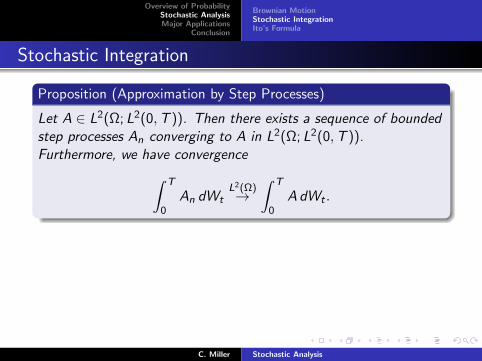
Proposition (Approximation by Step Processes)
Let A ∈ L2(Ω; L2(0,T )). Then there exists a sequence of boundedstep processes An converging to A in L2(Ω; L2(0,T )).Furthermore, we have convergence∫ T
0An dWt
L2(Ω)→∫ T
0A dWt .
Remark: There are myriad measurability issues we are glossingover. Typically, we ask that A : Ω× [0,T ]→ R is:
Square-integrable
”Progressively measurable”
”Adapted” + continuous, or ”predictable”
In this case, the Ito integral of A is a martingale.
C. Miller Stochastic Analysis

Overview of ProbabilityStochastic AnalysisMajor Applications
Conclusion
Brownian MotionStochastic IntegrationIto’s Formula
Stochastic Integration
Proposition (Approximation by Step Processes)
Let A ∈ L2(Ω; L2(0,T )). Then there exists a sequence of boundedstep processes An converging to A in L2(Ω; L2(0,T )).Furthermore, we have convergence∫ T
0An dWt
L2(Ω)→∫ T
0A dWt .
Remark: There are myriad measurability issues we are glossingover. Typically, we ask that A : Ω× [0,T ]→ R is:
Square-integrable
”Progressively measurable”
”Adapted” + continuous, or ”predictable”
In this case, the Ito integral of A is a martingale.C. Miller Stochastic Analysis

Overview of ProbabilityStochastic AnalysisMajor Applications
Conclusion
Brownian MotionStochastic IntegrationIto’s Formula
Ito’s Formula
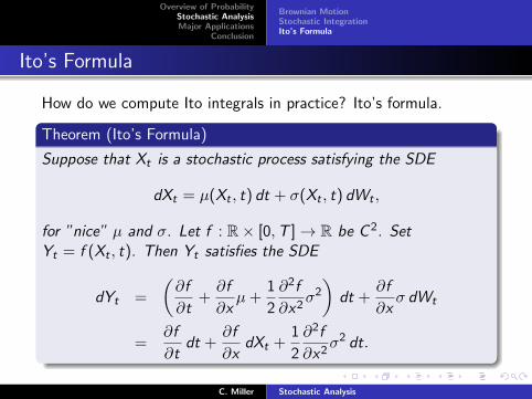
How do we compute Ito integrals in practice? Ito’s formula.
Theorem (Ito’s Formula)
Suppose that Xt is a stochastic process satisfying the SDE
dXt = µ(Xt , t) dt + σ(Xt , t) dWt ,
for ”nice” µ and σ. Let f : R× [0,T ]→ R be C 2. SetYt = f (Xt , t). Then Yt satisfies the SDE
dYt =
(∂f
∂t+∂f
∂xµ+
1
2
∂2f
∂x2σ2
)dt +
∂f
∂xσ dWt
=∂f
∂tdt +
∂f
∂xdXt +
1
2
∂2f
∂x2σ2 dt.
C. Miller Stochastic Analysis
Overview of ProbabilityStochastic AnalysisMajor Applications
Conclusion
Brownian MotionStochastic IntegrationIto’s Formula
Ito’s Formula
How do we compute Ito integrals in practice? Ito’s formula.
Theorem (Ito’s Formula)
Suppose that Xt is a stochastic process satisfying the SDE
dXt = µ(Xt , t) dt + σ(Xt , t) dWt ,
for ”nice” µ and σ. Let f : R× [0,T ]→ R be C 2. SetYt = f (Xt , t). Then Yt satisfies the SDE
dYt =
(∂f
∂t+∂f
∂xµ+
1
2
∂2f
∂x2σ2
)dt +
∂f
∂xσ dWt
=∂f
∂tdt +
∂f
∂xdXt +
1
2
∂2f
∂x2σ2 dt.
C. Miller Stochastic Analysis

Overview of ProbabilityStochastic AnalysisMajor Applications
Conclusion
Brownian MotionStochastic IntegrationIto’s Formula
Ito’s Formula
Lemma
1 d(W 2
t
)= dt + 2Wt dWt
2 d (tWt) = Wt dt + t dWt
Proof.
Let 0 = t0 < t1 < · · · < tn = t. Approximate the Ito integral:
n−1∑k=0
2Wtk
(Wtk+1
−Wtk
)= W 2
tn −n∑
k=0
(Wtk+1
−Wtk
)2 P→W 2t − t.
Similar for (2).
C. Miller Stochastic Analysis

Overview of ProbabilityStochastic AnalysisMajor Applications
Conclusion
Brownian MotionStochastic IntegrationIto’s Formula
Ito’s Formula
Lemma (Ito Product Rule)
Let Xt and Yt satisfy:dXt = µ1 dt + σ1 dWt
dYt = µ2 dt + σ2 dWt .
Thend (XtYt) = Yt dXt + Xt dYt + σ1σ2 dt.
Proof.
Approximate by step processes. Use previous lemma. Be carefulabout convergence.
C. Miller Stochastic Analysis

Overview of ProbabilityStochastic AnalysisMajor Applications
Conclusion
Brownian MotionStochastic IntegrationIto’s Formula
Ito’s Formula
Theorem (Ito’s Formula)
Suppose that Xt is a stochastic process satisfying the SDE
dXt = µ(Xt , t) dt + σ(Xt , t) dWt ,
for ”nice” µ and σ. Let f : R× [0,T ]→ R be C 2. SetYt = f (Xt , t). Then Yt satisfies the SDE
dYt =∂f
∂tdt +
∂f
∂xdXt +
1
2
∂2f
∂x2σ2 dt.
Proof.
Apply lemmas inductively to compute d(tnXmt ). Approximate f ,
∂f∂x , ∂2f
∂x2 , and ∂f∂t by polynomials. Be careful about convergence.
C. Miller Stochastic Analysis

Overview of ProbabilityStochastic AnalysisMajor Applications
Conclusion
Martingale Representation TheoremFeynman-Kac FormulaHamilton-Jacobi-Bellman Equation
Martingale Representation Theorem
Theorem
Let Wt be a Brownian motion with filtration Ft . Let Mt be acontinuous, square-integrable martingale with respect to Ft , alongwith a few other technical, but reasonable, conditions. Then thereexists a predictable process φt such that:
Mt = M0 +
∫ t
0φs dWs .
Significance:
Brownian motion is the archetypal continuous,square-integrable martingale.
C. Miller Stochastic Analysis
Overview of ProbabilityStochastic AnalysisMajor Applications
Conclusion
Martingale Representation TheoremFeynman-Kac FormulaHamilton-Jacobi-Bellman Equation
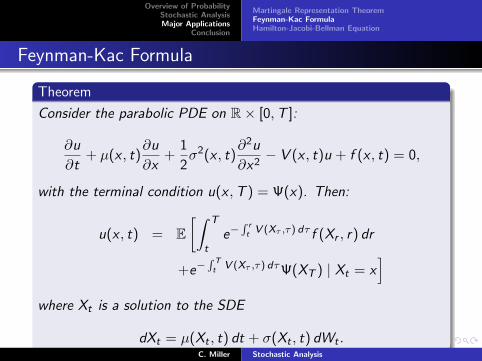
Feynman-Kac Formula
Theorem
Consider the parabolic PDE on R× [0,T ]:
∂u
∂t+ µ(x , t)
∂u
∂x+
1
2σ2(x , t)
∂2u
∂x2− V (x , t)u + f (x , t) = 0,
with the terminal condition u(x ,T ) = Ψ(x). Then:
u(x , t) = E[∫ T
te−
∫ rt V (Xτ ,τ) dτ f (Xr , r) dr
+e−∫ Tt V (Xτ ,τ) dτΨ(XT ) | Xt = x
]where Xt is a solution to the SDE
dXt = µ(Xt , t) dt + σ(Xt , t) dWt .C. Miller Stochastic Analysis

Overview of ProbabilityStochastic AnalysisMajor Applications
Conclusion
Martingale Representation TheoremFeynman-Kac FormulaHamilton-Jacobi-Bellman Equation
Feynman-Kac Formula
Proof.
Define a stochastic process:
Yr = e−∫ rt V (Xτ ,τ) dτu(Xr , r) +
∫ r
te−
∫ st V (Xτ ,τ) dτ f (Xs , s) ds.
Apply Ito’s formula, use the PDE to cancel a lot of terms, and get:
YT = Yt +
∫ T
te−
∫ st V (Xτ ,τ) dτσ(Xs , s)
∂u
∂xdWs .
Taking conditional expectations on each side and using themartingale-property of Ito integrals, we get:
u(x , t) = E [Yt | Xt = x ] = E [YT | Xt = x ] .
C. Miller Stochastic Analysis

Overview of ProbabilityStochastic AnalysisMajor Applications
Conclusion
Martingale Representation TheoremFeynman-Kac FormulaHamilton-Jacobi-Bellman Equation
Hamilton-Jacobi-Bellman Equation
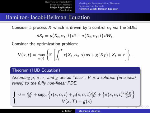
Consider a process X which is driven by a control αt via the SDE:
dXt = µ(Xt , αt , t) dt + σ(Xt , αt , t) dWt .
Consider the optimization problem:
V (x , t) = maxα(·)
E[∫ T
tr(Xs , αs , s) ds + g(XT ) | Xt = x
].
Theorem (HJB Equation)
Assuming µ, σ, r , and g are all ”nice”, V is a solution (in a weaksense) to the fully non-linear PDE:
0 = ∂V∂t + supα
r(x , α, t) + µ(x , α, t)∂V∂x + 1
2σ(x , α, t)2 ∂2V∂x2
V (x ,T ) = g(x)
C. Miller Stochastic Analysis
Overview of ProbabilityStochastic AnalysisMajor Applications
Conclusion
Martingale Representation TheoremFeynman-Kac FormulaHamilton-Jacobi-Bellman Equation
Hamilton-Jacobi-Bellman Equation
Consider a process X which is driven by a control αt via the SDE:
dXt = µ(Xt , αt , t) dt + σ(Xt , αt , t) dWt .
Consider the optimization problem:
V (x , t) = maxα(·)
E[∫ T
tr(Xs , αs , s) ds + g(XT ) | Xt = x
].
Theorem (HJB Equation)
Assuming µ, σ, r , and g are all ”nice”, V is a solution (in a weaksense) to the fully non-linear PDE:
0 = ∂V∂t + supα
r(x , α, t) + µ(x , α, t)∂V∂x + 1
2σ(x , α, t)2 ∂2V∂x2
V (x ,T ) = g(x)
C. Miller Stochastic Analysis

Overview of ProbabilityStochastic AnalysisMajor Applications
Conclusion
Martingale Representation TheoremFeynman-Kac FormulaHamilton-Jacobi-Bellman Equation
Hamilton-Jacobi-Bellman Equation
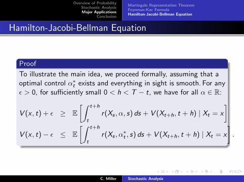
Proof
To illustrate the main idea, we proceed formally, assuming that aoptimal control α∗t exists and everything in sight is smooth.
For anyε > 0, for sufficiently small 0 < h < T − t, we have for all α ∈ R:
V (x , t) + ε ≥ E[∫ t+h
tr(Xs , α, s) ds + V (Xt+h, t + h) | Xt = x
]V (x , t)− ε ≤ E
[∫ t+h
tr(Xs , α
∗t , s) ds + V (Xt+h, t + h) | Xt = x
].
C. Miller Stochastic Analysis
Overview of ProbabilityStochastic AnalysisMajor Applications
Conclusion
Martingale Representation TheoremFeynman-Kac FormulaHamilton-Jacobi-Bellman Equation
Hamilton-Jacobi-Bellman Equation
Proof
To illustrate the main idea, we proceed formally, assuming that aoptimal control α∗t exists and everything in sight is smooth. For anyε > 0, for sufficiently small 0 < h < T − t, we have for all α ∈ R:
V (x , t) + ε ≥ E[∫ t+h
tr(Xs , α, s) ds + V (Xt+h, t + h) | Xt = x
]V (x , t)− ε ≤ E
[∫ t+h
tr(Xs , α
∗t , s) ds + V (Xt+h, t + h) | Xt = x
].
C. Miller Stochastic Analysis

Overview of ProbabilityStochastic AnalysisMajor Applications
Conclusion
Martingale Representation TheoremFeynman-Kac FormulaHamilton-Jacobi-Bellman Equation
Hamilton-Jacobi-Bellman Equation
Then, we conclude:
2ε ≥ |V (x , t)−supα
E[∫ t+h
tr(Xs , α, s) ds + V (Xt+h, t + h) | Xt = x
]|.
Applying Ito’s formula to the term inside the expectation, we see:∫ t+h
tr(Xs , α, s) ds + V (Xt+h, t + h)
= V (Xt , t) +
∫ t+h
t
(r +
∂V
∂t+ µ
∂V
∂x+
1
2σ2∂
2V
∂x2
)ds
+
∫ t+h
t· · · dWs .
C. Miller Stochastic Analysis

Overview of ProbabilityStochastic AnalysisMajor Applications
Conclusion
Martingale Representation TheoremFeynman-Kac FormulaHamilton-Jacobi-Bellman Equation
Hamilton-Jacobi-Bellman Equation
Now, using the martingale property of Ito integrals, we obtain:
2ε ≥ |supα
E[∫ t+h
t
(r +
∂V
∂t+ µ
∂V
∂x+
1
2σ2∂
2V
∂x2
)ds | Xt = x
]|.
Then taking ε, h→ 0, we obtain:
0 =∂V
∂t+ sup
α
r(x , α, t) + µ(x , α, t)
∂V
∂x+
1
2σ(x , α, t)2∂
2V
∂x2
.
C. Miller Stochastic Analysis

Overview of ProbabilityStochastic AnalysisMajor Applications
Conclusion
Conclusion
Stochastic analysis provides a mathematical framework foruncertainty quantification and local descriptions of globalstochastic phenomena.
Deep connections to elliptic and parabolic PDE,
Characterizes large classes of continuous-time stochasticprocesses,
Fundamental tools for the working analyst.
C. Miller Stochastic Analysis

Overview of ProbabilityStochastic AnalysisMajor Applications
Conclusion
C. Miller Stochastic Analysis