INTRODUCTION TO SOCIAL MACRODYNAMICS: Compact Macromodels of the World System

Andrey KorotayevArtemy Malkov

Daria Khaltourina

INTRODUCTION

TO SOCIAL MACRODYNAMICS:

Compact Macromodels

of the World System Growth

Moscow: URSS, 2006

RUSSIAN STATE UNIVERSITY FOR THE HUMANITIESFaculty of History, Political Science and Law

RUSSIAN ACADEMY OF SCIENCESCenter for Civilizational and Regional Studies

Institute of Oriental Studies

Andrey KorotayevArtemy Malkov

Daria Khaltourina

INTRODUCTION

TO SOCIAL MACRODYNAMICS:Compact Macromodels of

the World System Growth

Moscow: URSS, 2006

ББК 22.318

This study has been supported by the Russian Foundationfor the Fundamental Research

(Projects # 04–06–8022 and # 02-06-80260)

Korotayev Andrey, Malkov Artemy,Khaltourina Daria

Introduction to Social Macrodynamics: Compact Macromodels of the WorldSystem Growth. – Moscow: Editorial URSS, 2006. – 128 p.

ISBN 5–

Human society is a complex nonequilibrium system that changes and developsconstantly. Complexity, multivariability, and contradictoriness of social evolution leadresearchers to a logical conclusion that any simplification, reduction, or neglect of themultiplicity of factors leads inevitably to the multiplication of error and to significantmisunderstanding of the processes under study. The view that any simple general lawsare not observed at all with respect to social evolution has become totally predominantwithin the academic community, especially among those who specialize in the Humani-ties and who confront directly in their research all the manifold unpredictability of socialprocesses. A way to approach human society as an extremely complex system is to rec-ognize differences of abstraction and time scale between different levels. If the main taskof scientific analysis is to detect the main forces acting on systems so as to discover fun-damental laws at a sufficiently coarse scale, then abstracting from details and deviationsfrom general rules may help to identify measurable deviations from these laws in finerdetail and shorter time scales. Modern achievements in the field of mathematical model-ing suggest that social evolution can be described with rigorous and sufficiently simplemacrolaws.

This book discusses general regularities of the World System growth. It isshown that they can be described mathematically in a rather accurate way with rathersimple models.

Contents

Acknowledgements . . . . . . . . . . . . . . . . . . . . . . 4

Introduction . . . . . . . . . . . . . . . . . . . . . . . . . 5

Chapter 1 Macrotrends of World Population Growth . . . . . 10Chapter 2 A Compact Macromodel of

World Population Growth . . . . . . . . . . . 21Chapter 3 A Compact Macromodel of World Economic

and Demographic Growth . . . . . . . . . . 34Chapter 4 A General Extended Macromodel of World

Economic, Cultural, and Demographic Growth . . . 67Chapter 5 A Special Extended Macromodel of World

Economic, Cultural, and Demographic Growth . . . 81Chapter 6 Reconsidering Weber:

Literacy and "the Spirit of Capitalism" . . . . . . 87Chapter 7 Extended Macromodels

and Demographic Transition Mechanisms . . . . . 92

Conclusion . . . . . . . . . . . . . . . . . . . . . . 105

Appendices . . . . . . . . . . . . . . . . . . . . . . . . . . 112

Appendix 1 World Population Growth Forecast (2005–2050) . . 112Appendix 2 World Population Growth Rates and Female Literacy

in the 1990s: Some Observations . . . . . . . . 115Appendix 3 Hyperbolic Growth of the World Population and

Kapitza's Model . . . . . . . . . . . . . . . 118

Bibliography . . . . . . . . . . . . . . . . . . . . . . 124

Acknowledgements

First and foremost, our thanks go to the Institute for Advanced Study, Princeton.Without the first author's one-year membership in this Institute this book couldhardly have been written. We are also grateful to the Russian Foundation for BasicResearch for financial support of this work (projects # 04–06–8022 and # 02-06-80260).

We would like to express our special gratitude to Gregory Malinetsky, SergeyPodlazov (Institute for Applied Mathematics, Russian Academy of Sciences),Robert Graber (Truman State University), Victor de Munck (State University ofNew York), Duran Bell and Douglas R. White (University of California, Irvine)for their invaluable help and advice.

We would also like to thank our colleagues who offered us useful commentsand insights on the subject of this book: Leonid Alaev (Oriental Institute, RussianAcademy of Sciences), Herbert Barry III (University of Pittsburgh), Yuri Berzkin(Kunstkammer, St. Petersburg), Svetlana Borinskaya (Institute of GeneralGenetics, Russian Academy of Sciences), Dmitri Bondarenko (Institute forAfrican Studies, Russian Academy of Sciences), Michael L. Burton (University ofCalifornia, Irvine), Robert L. Carneiro (American Museum of Natural History,New York), Henry J. M. Claessen (Leiden University), Marina Butovskaya(Institute of Ethnology and Anthroplogy, Russian Academy of Sciences), DmitrijChernavskij (Institute of Physics, Russian Academy of Sciences), MaratCheshkov (Institute of International Economics, Russian Academy of Sciences),Loren Demerath (Centenary College), Georgi and Lubov Derlouguian(Northwestern University, Evanston), William T. Divale (City University of NewYork), Timothy K. Earle (Northwestern University), Leonid Grinin (Center forSocial and Historical Research, Volgograd), Eric C. Jones (University of NorthCarolina), Natalia Komarova (University of California, Irvine), Sergey Nefedov(Russian Academy of Sciences, Ural Branch, Ekaterinburg), Nikolay Kradin(Russian Academy of Sciences, Far East Branch, Vladivostok), Vitalij Meliantsev(Institute of Asia and Africa, Moscow State University), Akop Nazaretyan(Oriental Institute, Russian Academy of Sciences), Nikolay Rozov (NovosibirskState University), Igor Sledzevski (Institute for African Studies, Moscow), DavidSmall (Lehigh University), Peter Turchin (University of Connecticut, Storrs), andPaul Wason (Templeton Foundation).

Needless to say, faults, mistakes, infelicities, etc., are our own responsibility.

Introduction1

Human society is a complex nonequilibrium system that changes and developsconstantly. Complexity, multivariability, and contradictoriness of social evolu-tion lead researchers to a logical conclusion that any simplification, reduction,or neglect of the multiplicity of factors leads inevitably to the multiplication oferror and to significant misunderstanding of the processes under study. Theview that any simple general laws are not observed at all with respect to socialevolution has become totally predominant within the academic community, es-pecially among those who specialize in the Humanities and who confront direct-ly in their research all the manifold unpredictability of social processes.

A way to approach human society as an extremely complex system is to rec-ognize differences of abstraction and time scale between different levels. If themain task of scientific analysis is to detect the main forces acting on systems soas to discover fundamental laws at a sufficiently coarse scale, then abstractingfrom details and deviations from general rules may help to identify measurabledeviations from these laws in finer detail and shorter time scales. Modernachievements in the field of mathematical modeling suggest that social evolu-tion can be described with rigorous and sufficiently simple macrolaws. Ourgoal, at this stage, is to discuss a family of mathematical models whose greaterspecification leads to measurable variables and testable relationships.

Tremendous successes and spectacular developments in physics (especially,in comparison with other sciences) were, to a considerable degree, connectedwith the fact that physics managed to achieve a synthesis of mathematical me-thods and subject knowledge. Notwithstanding the fact that already in the clas-sical world physical theories achieved a rather high level, it was in the modernera that the introduction of mathematics made it possible to penetrate deeper in-to the essence of physical laws, laying the ground for the scientific-technological revolution. However, such a synthesis was not possible withoutone important condition. Mathematics operates with forms and numbers, and,hence, the physical world had to be translated into the language of forms andnumbers. It demanded the development of effective methods for measuringphysical values and the introduction of scales and measures. Starting with thesimplest variables – length, mass, time – physicists learned how to measure

1 This book is a translation of an amended and enlarged version of Part 1 of the following mono-graph originally published in Russian: Коротаев, А. В., А. С. Малков и Д. А. Хал-турина. Законы истории: Математическое моделирование исторических макропроцессов(Демография. Экономика. Войны). М.: УРСС, 2005.

Introduction6

charge, viscosity, inductance, spin and many other variables, which are neces-sary for the development of the physical theory of value.

In an analogous way, a constructive synthesis of the social sciences with ma-thematics calls for the introduction of adequate methods for the measurement ofsocial variables. In the social sciences, as in physics, some variables can bemeasured relatively easily, while the measurement of some other variablesneeds additional research and even the development of auxiliary models.

One social variable that is relatively well accessible to direct measurement ispopulation size. That is why it is not surprising that the field of demography at-tracts the special attention of social scientists, as it suggests some hope for thedevelopment of quantitatively based scientific theories. It is remarkable that thepenetration of mathematical methods into biology began, to a considerable ex-tent, with the description of population dynamics.

The basic measurability of data is quite evident here; what is more, the basicequation for the description of demographic dynamics is also rather evident, asit stems from the conservation law:

DBdtdN

, (0.1)

where N is the number of people, B is the number of births, and D is the numberof deaths in the unit of time. However, at the microlevel it turns out that boththe number of deaths and number of births depend heavily on a huge number ofsocial parameters, including the "human factor" – decisions made by individualpeople that are very difficult to formalize.

In addition to this, equation (0.1) does not take into account the spatialmovement of people; hence, it should be extended:

Jdiv DB

tN

, (0.1')

where vector J corresponds to the migration current. In this case the problembecomes even more complicated, as migration processes are even more likely tobe influenced by external factors.

That is why any formal description of demographic processes at the micro-level confronts serious problems associated first of all with the lack of sufficientresearch on formal social laws connecting economic, political, ethical and otherfactors that affect individual and small group (e.g., household or nuclear family)behavior. Thus, at the moment the only available approach is macrolevel de-scription that does not go into the fine details of demographic processes and de-

Introduction 7

scribes dynamics of very large human populations, which is influenced by thehuman factor at a significantly coarser level of abstraction and on a longer time-scale.

Biological processes of birth and death are characteristic not only of people,but also of any animals. That is why a rather natural step is to try to describedemographic models using population models developed within biology (see,e.g., Riznichenko 2002).

The basic model describing animal population dynamics is the logistic mod-el, suggested by Verhulst (1838):

)1(KNrN

dtdN

, (0.2)

which can be also presented in the following way:

)()( 221 bNNaNa

dtdN

, (0.3)

where a1N corresponds to the number of births B, and a2N + bN2 corresponds tothe number of deaths in equation (0.1); r, K, a1, a2, b are positive coefficientsconnected between themselves by the following relationships:

r = a1 – a2 and Krb , (0.4)

The logic of equation (0.3) is as follows: fertility a1 is a constant; thus, thenumber of births B = a1N is proportional to the population size, natural deathrate a2 is also considered to be constant, whereas quadratic addition bN2 in ex-pression for full number of deaths D = a1N+bN2 appears due to the resource li-mitation, which does not let population grow infinitely. Coefficient b is calledthe coefficient of interspecies competition.

As a result, the population dynamics described by the logistic equation hasthe following characteristics. At the beginning, when the size of the animalpopulation size is low, we observe an exponential growth with exponentr = a1 – a2. Then, as the ecological niche is being filled, the population growthslows down, and finally the population comes to the constant level K.

The value of parameter K, called the carrying capacity of an ecologicalniche for the given population, is of principal importance. This value deter-

Introduction8

mines the equilibrium state in population dynamics for the given resource limi-tations and controls the limits of its growth.

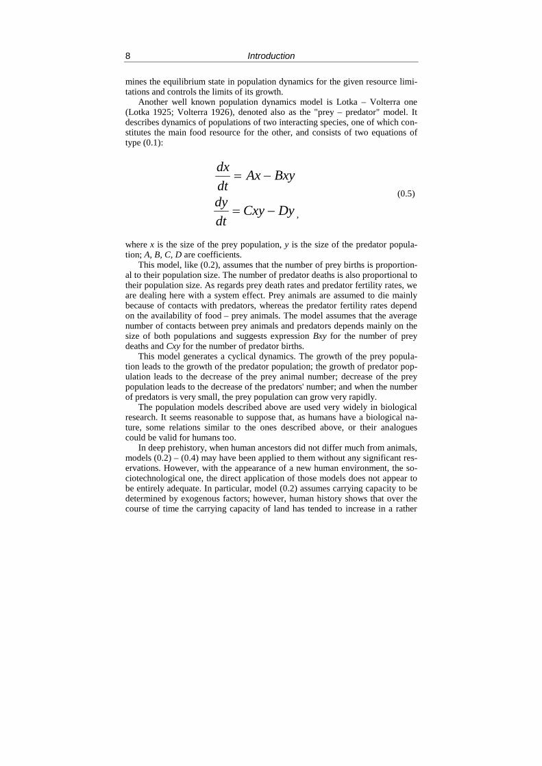
Another well known population dynamics model is Lotka – Volterra one(Lotka 1925; Volterra 1926), denoted also as the "prey – predator" model. Itdescribes dynamics of populations of two interacting species, one of which con-stitutes the main food resource for the other, and consists of two equations oftype (0.1):

BxyAxdtdx

DyCxydtdy

,

(0.5)

where x is the size of the prey population, y is the size of the predator popula-tion; A, B, C, D are coefficients.

This model, like (0.2), assumes that the number of prey births is proportion-al to their population size. The number of predator deaths is also proportional totheir population size. As regards prey death rates and predator fertility rates, weare dealing here with a system effect. Prey animals are assumed to die mainlybecause of contacts with predators, whereas the predator fertility rates dependon the availability of food – prey animals. The model assumes that the averagenumber of contacts between prey animals and predators depends mainly on thesize of both populations and suggests expression Bxy for the number of preydeaths and Cxy for the number of predator births.

This model generates a cyclical dynamics. The growth of the prey popula-tion leads to the growth of the predator population; the growth of predator pop-ulation leads to the decrease of the prey animal number; decrease of the preypopulation leads to the decrease of the predators' number; and when the numberof predators is very small, the prey population can grow very rapidly.

The population models described above are used very widely in biologicalresearch. It seems reasonable to suppose that, as humans have a biological na-ture, some relations similar to the ones described above, or their analoguescould be valid for humans too.

In deep prehistory, when human ancestors did not differ much from animals,models (0.2) – (0.4) may have been applied to them without any significant res-ervations. However, with the appearance of a new human environment, the so-ciotechnological one, the direct application of those models does not appear tobe entirely adequate. In particular, model (0.2) assumes carrying capacity to bedetermined by exogenous factors; however, human history shows that over thecourse of time the carrying capacity of land has tended to increase in a rather

Introduction 9

significant way. Hence, in long-range perspective carrying capacity cannot beassumed to be constant and determined entirely by exogenous conditions. Hu-mans are capable of transforming those conditions affecting carrying capacity.

As regards model (0.4), it has an extremely limited applicability to humansin its direct form, as humans learned how to defend themselves effectively frompredators at very early stages of their evolution; hence, humans cannot functionas "prey" in this model. On the other hand, humans learned how not to dependon the fluctuations of prey animals populations, hence, they cannot function aspredators because in model (0.4) predators are very sensitive to the variations ofprey animal numbers (This model could still have some limited direct applica-bility to a very few cases of highly specialized hunters).

However, model (0.4) may find a new non-traditional application in demo-graphic models. In particular it may be applied to the description of demograph-ic cycles that have been found in historical dynamics of almost all the agrariansocieties, for which relevant data are available. The population plays here therole of "prey", whereas the role of "predator" belongs to sociopolitical instabili-ty, internal warfare, famines and epidemics whose probability increases when anincreasing population approaches the carrying capacity ceiling (for detail see,e.g., Korotayev, Malkov and Khaltourina 2005: 211–54). Demographic cyclesare by themselves a very interesting subject for mathematical research, and theyhave been studied rather actively in recent years (Usher 1989; Chu and Lee1994; Malkov and Sergeev 2002, 2004; Malkov et al. 2002; Malkov 2002,2003, 2004; Malkov, Selunskaja, and Sergeev 2005; Turchin 2003, 2005a,2005b; Turchin and Korotayev 2006; Nefedov 2002a; 2004; Korotayev, Mal-kov and Khaltourina 2005 etc.)

As is well known in complexity studies, chaotic dynamics at the microlevelcan generate a highly deterministic macrolevel behavior (e.g., Chernavskij2004). To describe behavior of a few dozen gas molecules in a closed vessel weneed very complex mathematical models; and these models would still be una-ble to predict long-run dynamics of such a system due to inevitable irreduciblechaotic components. However, the behavior of zillions of gas molecules can bedescribed with extremely simple sets of equations, which are capable of predict-ing almost perfectly the macrodynamics of all the basic parameters (just be-cause of chaotic behavior at microlevel). Of course, one cannot fail to wonderwhether a similar set of regularities would not also be observed in the humanworld too. That is, cannot a few very simple equations account for an extremelyhigh proportion of all the macrovariation with respect to the largest possible so-cial system – the World System?

Chapter 1

Macrotrends ofWorld Population Growth

The world population growth in 1950–2003 had the following shape (see Dia-gram 1.11):

Diagram 1.1. World Population Growth, 1950–2003 (millions)

0

1000

2000

3000

4000

5000

6000

7000

1940 1950 1960 1970 1980 1990 2000 2010

Though at first glance world population growth in 1950–2003 looks almost per-fectly linear, even a very simple analysis of the dynamics of annual growth ratesindicates that the actual situation is far more complex (see Table 1.1 and Dia-gram 1.2):

1 The world population dynamics data for 1950–2003 are here and elsewhere from US Census Bu-reau database (2004).

Macrotrends of World Population Growth 11

Table 1. World Population Dynamics, 1950–2003

Year Population Annual growth rate(%)

Annual populationchange

1950 2,555,360,972 1.47 37,785,9861951 2,593,146,958 1.61 42,060,3891952 2,635,207,347 1.71 45,337,2321953 2,680,544,579 1.77 47,971,8231954 2,728,516,402 1.87 51,451,6291955 2,779,968,031 1.89 52,959,3081956 2,832,927,339 1.95 55,827,0501957 2,888,754,389 1.94 56,506,5631958 2,945,260,952 1.76 52,335,1001959 2,997,596,052 1.39 42,073,2781960 3,039,669,330 1.33 40,792,1721961 3,080,461,502 1.80 56,094,5901962 3,136,556,092 2.19 69,516,1941963 3,206,072,286 2.19 71,119,8131964 3,277,192,099 2.08 69,031,9821965 3,346,224,081 2.08 70,238,8581966 3,416,462,939 2.02 69,755,3641967 3,486,218,303 2.04 71,882,4061968 3,558,100,709 2.08 74,679,9051969 3,632,780,614 2.05 75,286,4911970 3,708,067,105 2.07 77,587,0011971 3,785,654,106 2.01 76,694,6601972 3,862,348,766 1.95 76,183,2831973 3,938,532,049 1.90 75,547,2181974 4,014,079,267 1.81 73,271,8281975 4,087,351,095 1.74 71,804,5691976 4,159,155,664 1.72 72,229,6961977 4,231,385,360 1.69 72,172,0751978 4,303,557,435 1.73 75,085,8581979 4,378,643,293 1.72 75,746,226

Chapter 112

Year Population Annual growth rate(%)

Annual populationchange

1980 4,454,389,519 1.68 75,430,3531981 4,529,819,872 1.74 79,706,2831982 4,609,526,155 1.75 81,444,4231983 4,690,970,578 1.70 80,459,7091984 4,771,430,287 1.70 81,822,3761985 4,853,252,663 1.71 83,561,3681986 4,936,814,031 1.73 86,175,6011987 5,022,989,632 1.71 86,843,5111988 5,109,833,143 1.69 86,965,2351989 5,196,798,378 1.68 87,880,7451990 5,284,679,123 1.58 84,130,4981991 5,368,809,621 1.56 84,182,0871992 5,452,991,708 1.49 81,942,2471993 5,534,933,955 1.44 80,547,5321994 5,615,481,487 1.43 80,781,9741995 5,696,263,461 1.38 79,253,6221996 5,775,517,083 1.37 79,551,0741997 5,855,068,157 1.32 78,019,0391998 5,933,087,196 1.29 76,861,7161999 6,009,948,912 1.25 75,529,8662000 6,085,478,778 1.21 74,220,5282001 6,159,699,306 1.18 73,002,8632002 6,232,702,169 1.16 72,442,5112003 6,305,144,680 1.14 72,496,962


Diagram 1.2. Dynamics of Annual World Population Growth,1950–2003 (%)

1950

1952

1957

1962

19671972

19771982 1987

1992

1997

2003

0

0.5

1

1.5

2

2.5

1950 1960 1970 1980 1990 2000 2010

As we see, before 1962 one can observe a rather rapid increase of populationgrowth rates. However after 1963 we encounter a clear-cut reverse trend – theannual growth rates tend to decrease rather steadily and fast. In fact in 1990–2003 we observe an extremely strong negative correlation between world popu-lation and world population growth rates (see Diagram 1.3):

Chapter 114

Diagram 1.3. Correlation between World Population Size andWorld Population Annual Growth Rate, 1990–2003

World Population (millions)

6400620060005800560054005200

An

nu

al W

orl

d P

op

ula

tio

n G

row

th R

ate

(%

)

1.7

1.6

1.5

1.4

1.3

1.2

1.1

20032002

20012000

1999

19981997

19961995

19941993

1992

19911990

Regression analysis of this dataset gives the following results (see Table 1.2):


Table 1.2. Correlation between World Population Size andWorld Population Annual Growth Rate, 1990–2003(regression analysis)

UnstandardizedCoefficients

Standardized Coeffi-cients t Sig.

Model B Std. Error Beta

1(Constant) 3.903 0.064 61.290 0.0000000000000003World Popula-tion (billions)

-0.441 0.011 -0.996 -40.259 0.00000000000004

Dependent Variable: World Population Annual Growth Rate (%)

NOTE: R = 0.996, R2 = 0.993.

This, of course, suggests that 99.3% of all the world macrodemographic varia-tion in 1990–2003 is predicted by the following extremely simple equation:

r = 3.9 – 0.44N , (1.1)

where N is the world population in billions, and r is the annual populationgrowth rate (%).

Naturally, this makes it possible to estimate what the future population ofthe world will be if the recent pattern of relationships between N and r persists,using the following equation (Model 1):

Model 1Ni+1 = Ni (1 + [3.9 – 0.44Ni]/100)

The results of respective simulation starting in 2003 with N = 6,305,144,680look as follows (see Table 1.3 and Diagram 1.4):

Table 1.3. Future Population (millions) of the World,estimates produced with Model 1 simulation

Year 2010 2020 2030 2040 2050 2060 2070Population 6785.6 7360.3 7801.6 8126.0 8356.8 8517.2 8626.8Year 2080 2090 2100 2110 2120 2130 2150Population 8700.9 8750.6 8783.8 8805.8 8820.5 8830.2 8840.8

Chapter 116

Diagram 4. World Population (millions) in 1950–2003,with Extrapolation of 1990–2003 Dynamic Trend till 2150

0

1000

2000

3000

4000

5000

6000

7000

8000

9000

10000

1950 2000 2050 2100 2150

How likely is it that actual world population growth will follow this pattern? Aswe shall see, there are strong theoretical and empirical grounds to maintain thatin no way is this entirely unlikely.

To start with, the pattern of strong linear relationship between world popula-tion size and world population growth rate observed for 1990–2003 is in noway unique for the world's demographic history. In fact, just this pattern pre-vailed for most of human history, at least within the last two millennia (e.g.,Kapitza 1992, 1999; Kremer 1993). For example, for 1650–1960 this relation-ship looks as follows (see Table 1.4 and Diagram 1.5):


Table 1.4. World Population Macrodynamics, 1650–2003

PeriodWorld Populationat the beginning of

the Period (millions)

Average AnnualGrowth Rate during theRespective Period (%)

1650-1700 545.0 0.22531700-1750 610.0 0.33161750-1800 720.0 0.44631800-1850 900.0 0.57541850-1875 1200.0 0.39641875-1900 1325.0 0.81641900-1920 1625.0 0.83061920-1930 1813.0 0.91641930-1940 1987.0 1.07771940-1950 2213.0 1.28321950-1960 2555.4 1.82261960-1970 3039.7 2.0151

NOTE: estimates by (Kremer 1993: 683).

Diagram 1.5. Correlation between World Population Size andWorld Population Annual Growth Rate, 1650–1970

World Population (millions)

40003000200010000

Annu

al G

row

th R

ate

(%)

2.5

2.0

1.5

1.0

.5

0.0

1960-70

1950-60

1940-50

1930-40

1920-3019001875-900

1850-75

1800-501750-8001700-501650-1700

Chapter 118

Regression analysis of Kremer's dataset for 1650–1970 produces the followingresults (see Table 1.5):

Table 1.5. Correlation between World Population Size andWorld Population Annual Growth Rate, 1650–1970(regression analysis)


StandardizedCoefficients t Sig.

Model B Std. Error Beta

2(Constant) -0.172 0.099 -1.744 0.112World Population (billions) 0.691 0.057 0.967 12.074 0.0000003


NOTE: R = 0.967, R2 = 0.936 (for 1900-1970 R = 0.981, R2 = 0.962)

This, of course, suggests that 93.6% of all the world macrodemographic varia-tion in 1650–1970 is predicted by another simple equation (Model 2):

r = 0.69N – 0.17,

where N is the world population in billions, and r is the annual populationgrowth rate.

On the other hand, 96.2 % of all the world macrodemographic variation in1900–1970 is predicted by Model 3 arrived at through a similar regressionanalysis of data for this period:

r = 0.92N – 0.71 .

Thus, very strong and rather uniform linear relationship between world popula-tion size and annual growth rate can be observed in historical record for dec-ades and even centuries.

Combining our extrapolation of 1990-2003 world population with the dataon world population growth from 500 BCE till 2003 (Kremer 1993; US Bureauof the Census 2004)2 we arrive at the following picture (see Diagram 1.6):

2 The other sources consulted are: Thomlinson 1975; Durand 1977; McEvedy and Jones 1978:342–51; Biraben 1980; Haub 1995: 5; UN Population Division 2004; World Bank 2004.


Diagram 1.6. World Population Growth, 500 BCE – 2300 CE, millions

0

1000

2000

3000

4000

5000

6000

7000

8000

9000

10000

-500 0 500 1000 1500 2000 2500

In fact there is only one really significant difference in the patterns of worldpopulation growth observed in 1990–2003, on the one hand, and in the pre-1962/3 era, on the other. In 1990–2003 we observe a very strong NEGATIVEcorrelation between world population size and annual growth rates. For the pre-1962/3 era we also find a very strong correlation between those two variables.But this correlation is POSITIVE.

Naturally, this means that the long-run world population growth trend in thepre-1962/3 era was HYPERBOLIC. The hyperbolic population growth implies

Chapter 120

that the absolute population growth is proportional to the square of population(unlike exponential growth when the absolute growth is lineally proportional topopulation). Thus, with the exponential growth if at the world population levelof 100 million the absolute annual growth was 100 thousand people a year, at 1billion level it will be 1 million people a year (a ten times growth of populationleads to an equivalent 10 times increase in the absolute population growth). Forhyperbolic growth, if at the world population level of 100 million the absoluteannual growth was 100 thousand people a year, at 1 billion level it will be 10million people a year (the ten times growth of population leads to a 100 timesincrease in the absolute population growth rate). Note that the relative popula-tion growth rate will remain constant with the exponential growth (0.1% in ourexample), whereas it will be lineally proportional to absolute population levelwith hyperbolic growth (in our example the population growth by a factor of 10leads to the increase in the relative annual growth rate 10 times, from 0.1% to1%). Respectively, the world population growth trend observed in 1990–2003can be identified as INVERSE HYPERBOLIC (or just logistic).

Chapter 2

A Compact Macromodel ofWorld Population Growth

The fact that up to the 1960s world population growth had been characterizedby a hyperbolic trend was discovered quite long ago (see, e.g., von Foerster,Mora, and Amiot 1960; von Hoerner 1975; Kremer 1993; Kapitza 1992, 1999,etc.). In 1960 von Foerster, Mora, and Amiot conducted a statistical analysis ofthe available world population data and found out that the general shape of theworld population (N) growth is best approximated by the curve described by thefollowing equation:

ttCN

0

, (2.1)

where C and t0 are constants, whereas t0 corresponds to an absolute limit of sucha trend at which N would become infinite, and thus logically implies the certain-ty of the empirical conclusion that further increases in the growth trend willcease well before that date, which von Foerster wryly called the "doomsday"implication of power-law growth (he refers tongue-in-cheek to the estimated t0as "Doomsday, Friday, 13 November, A.D. 2026").

Von Foerster, Mora, and Amiot try to account for their empirical observa-tions by modifying the usual starting equations (0.1) and (0.3) for populationdynamics, so as to describe the process under consideration:

DBdtdN

, (0.1)

where N is the number of people, B is the number of births, and D is the numberof deaths in the unit of time;

Chapter 222

)()( 221 bNNaNa

dtdN

, (0.3)

where a1N corresponds to the number of births B, and a2N + bN2 corresponds tothe number of deaths in equation (0.1); let us recollect that r, K, a1, a2, b arepositive coefficients connected between themselves by the following relation-ships:

r = a1 – a2 and Krb , (0.4)

They start with the observation that when individuals in a population compete ina limited environment, the growth rate typically decreases with the greaternumber N in competition. This situation would typically apply where sufficientcommunication is lacking to enable resort to other than a competitive and nearlyzero-sum multiperson game. It might not apply, they suppose, when the ele-ments in a population "possess a system of communication which enables themto form coalitions" and especially when "all elements are so strongly linked thatthe population as a whole can be considered from a game-theoretical point ofview as a single person playing a two-person game with nature as the opponent"(von Foerster, Mora, and Amiot 1960: 1292). Thus, the larger the population(Nk coalition members, where k < 1) the more the decrease of natural risks andthe higher the population growth rate. They suggest modeling such a situationthrough the introduction of nonlinearity in the following form:

NNadtdN k )(

1

0 ,(2.2)

where a0 and k are constants, which should be determined experimentally. Theanalysis of experimental data by von Foerster, Mora, and Amiot determinesvalues a0 = 5.5×10-12 and k = 0.99 that produce the hyperbolic equation forworld population growth:

k

ttttNN

0

101 ,

(2.3)

A Compact Macromodel of World Population Growth 23

which, assuming k = 1.0 (von Hoerner1975) is written more succinctly as (2.1)and in equivalent form (Kapitza 1992, 1999) as (2.4):1

CN

dtdN 2

. (2.4)

Though von Foerster's, von Hoerner's and Kapitza's models produce a pheno-menal fit with the empirical data, they do not account for mechanisms of thehyperbolic trend; as we shall see in the next chapter, Kremer's (1993) model ac-counts for it, but it is rather complex. In fact, the general shape of world popula-tion growth dynamics could be accounted for with strikingly simple models likethe one we would like to propose ourselves below (or the model proposed byTsirel [2004]).2

With Kremer (1993), Komlos, Nefedov (2002) and others (Habakkuk 1953;Postan 1950, 1972; Braudel 1973; Abel 1974, 1980; Cameron 1989; Artzrouniand Komlos 1985 etc.), we make "the Malthusian (1978) assumption that popu-lation is limited by the available technology, so that the growth rate of popula-tion is proportional to the growth rate of technology" (Kremer 1993: 681–2),3and that, on the other hand, "high population spurs technological change be-cause it increases the number of potential inventors…4 In a larger populationthere will be proportionally more people lucky or smart enough to come up withnew ideas"5 (Kremer 1993: 685), thus, "the growth rate of technology is propor-tional to total population"6 (Kremer 1993: 682; see also, e.g., Kuznets 1960;Grossman and Helpman 1991; Aghion and Howitt 1992, 1998; Simon 1977,1981, 2000; Komlos and Nefedov 2002; Jones 1995, 2003, 2005 etc.).

1 See Appendix 3 for more detail.2 For other models of the world population hyperbolic growth see Cohen 1995; Johansen and

Sornette 2001; Podlazov 2004.3 In addition to this, the absolute growth rate is proportional to population itself – with the given

relative growth rate a larger population will increase more in absolute numbers than a smallerone.

4 "This implication flows naturally from the nonrivalry of technology… The cost of inventing anew technology is independent of the number of people who use it. Thus, holding constant theshare of resources devoted to research, an increase in population leads to an increase in technolo-gical change" (Kremer 1993: 681).

5 The second assumption is in fact Boserupian rather than Malthusian (Boserup 1965; Lee 1986).6 Note that "the growth rate of technology" means here the relative growth rate (i.e., the level to

which technology will grow in the given unit of time in proportion to the level observed at thebeginning of this period). This, of course, implies that the absolute speed of technology growth inthe given period of time will be proportional not only to the population size, but also to the abso-lute technology level at the beginning of this period.

Chapter 224

The simplest way to model mathematically the relationships between thesetwo subsystems (which, up to our knowledge, has not yet been proposed)7 is touse the following set of differential equations:

NNbKadtdN )( , (2.5)

cNKdtdK , (2.6)

where N is the world population, K is the level of technology; bK correspondsto the number of people (N), which the earth can support with the given level oftechnology (K). With such a compact model we are able to reproduce ratherwell the long-run hyperbolic growth of world population before 1962-3.

With our two-equation model we start the simulation in the year 1650 anddo annual iterations with difference equations derived from the differentialones:

Ki+1 = Ki + cNiKi ,Ni+1 = Ni + a(bKi+1 – Ni)Ni .

We choose the following values for the constants and initial conditions:N = 0.0545 of tens of billions (i.e. 545 million)8; a = 1; b = 1; K = 0.0545;9

c = 0.05135. The outcome of the simulation, presented in Diagrams 2.1–2 indi-cates that irrespective of its simplicity the model is actually capable of replicat-ing quite reasonably the population estimates of Kremer (1993), US Bureau ofthe Census (2004) and other sources (Thomlinson 1975; Durand 1977; McEve-dy and Jones 1978: 342–51; Biraben 1980; Haub 1995: 5; UN Population Divi-sion 2005; World Bank 2005) in most of their characteristics and in terms of theimportant turning points:

7 The closest proposed model is the one by Tsirel (2004); see our discussion of this very interestingmodel in Korotayev, Malkov, and Khaltourina 2005: 38–57.

8 We chose to calculate the world population in tens of billions (rather than, say, in millions) tominimize the rounding error stemming from discrete computer nature (which was to be takenmost seriously into account in our case, as the object of modeling had evident characteristics of ablow-up regime).

9 To simplify the calculations we chose value "1" for both a and b; thus, K in our simulations wasmeasured directly as the number of people which can be supported by the Earth with the givenlevel of technology.


Diagram 2.1. Predicted and Observed Dynamicsof the World Population Growth,in millions (1650–1962 CE)

0

500

1000

1500

2000

2500

3000

3500

1600 1650 1700 1750 1800 1850 1900 1950 2000

NOTE: The solid grey curve has been generated by the model; black markers correspond to the es-timates of world population by Kremer (1993) for pre-1950 period, and US Bureau of Census(2005) world population data for 1950–1962.

The correlation between the predicted and observed values for this simulationlooks as follows: R = 0.9989, R2 = 0.9978, p << 0.0001, which, of course, indi-cate an unusually high fit for such a simple model designed to account for de-mographic macrodynamics of the most complex social system (see Dia-gram 2.2):

Chapter 226

Diagram 2.2. Correlation between Predicted and Observed Values(1650–1962)

World Population Predicted by the Model

3200280024002000160012008004000

Ob

se

rve

d W

orl

d P

op

ula

tio

n

3200

2800

2400

2000

1600

1200

800

400

0

We start our second simulation in the year 500 BCE. In this case we choose thefollowing values of the constants and initial conditions: N = 0.01 of tens of bil-lions (i.e. 100 million); a = 1; b = 1; K = 0.01; c = 0.04093. The outcome of thesimulation, presented in Diagrams 2.3–4 indicates that irrespective of its ex-treme simplicity the model is still quite capable of replicating rather reasonablythe population estimates of Kremer (1993), US Bureau of the Census (2004)and other sources in most of their characteristics and in terms of the importantturning points even for such a long period of time:


Diagram 2.3. Predicted and Observed Dynamicsof the World Population Growth,in millions (500 BCE – 1962 CE)

0

500

1000

1500

2000

2500

3000

3500

-500 0 500 1000 1500 2000

NOTE: The solid grey curve has been generated by the model; black markers correspond to the es-timates of world population by Kremer (1993) for pre-1950 period, and US Bureau of Census(2005) world population data for 1950–1962.

The correlation between the predicted and observed values for this simulationlooks as follows: R = 0.9983, R2 = 0.9966, p << 0.0001, which, of course, againindicate an unusually high fit for such a simple model designed to account fordemographic macrodynamics of the most complex social system for c. 2500years (see Diagram 2.4):

Chapter 228

Diagram 2.4. Correlation between Predicted and Observed Values

World Population Predicted by the Model

3200280024002000160012008004000

Ob

serv

ed

Wo

rld

Po

pu

latio

n

3200

2800

2400

2000

1600

1200

800

400

0

Note that even when the simulation was started c. 25000 BCE, it still produceda fit with observed data as high as 0.981 (R2 = 0.962, p << 0.0001).10

Thus, it turns out that the set of two differential equations specified aboveaccounts for 96.2 per cent of all the variation in demographic macrodynamics ofthe world in the last 25 millennia; it also accounts for 99.66% of this macrovar-iation in 500 BCE – 1962 CE, and it does for 99.78% in 1650–1962 CE.

10 The simulation was started in the 24939 BCE and done with 269 centennial iterations ending in1962 CE. In this case we chose the following values of the constants and initial conditions:N = 0.00334 billion (i.e. 3.34 million); a = 1; b = 1; K = 0.00334; c = 2.13.


In fact, we believe this may not be a coincidence that the compact macro-model shows such a high correlation between the predicted and observed datajust for 500 BCE – 1962 CE. But why does the correlation significantly declineif the pre-500 BCE period is taken into account?

To start with, when we first encountered models of world populationgrowth, we felt a strong suspicion about them. Indeed, such models imply thatthe world population can be treated as a system. However, at a certain level ofanalysis one may doubt if this makes any sense at all. The fact is that up untilrecently (especially before 1492) humankind did not constitute any real system,as, for example. The growth of the Old World, New World, Australia, Tasma-nia, or Hawaii populations took place almost perfectly independently of eachother. For example, it seems entirely clear that demographic processes in, say,West Eurasia in the 1st millennium CE did not have the slightest impact on thedemographic dynamics of the Tasmanian population during the same time pe-riod.

However, we believe that the patterns observed in pre-Modern world popu-lation growth are not coincidental at all. In fact, they reflect population dynam-ics of quite a real entity, the World System. We are inclined to speak, with An-dre Gunder Frank (e.g., Frank and Gills 1994) but not with Wallerstein (1974),about a single World System which originated long before the "long 16th cen-tury".

Note that the presence of a more or less well integrated World System,comprising most of the world population, is a necessary pre-condition for thehigh correlation between the world population numbers generated by our modeland the observed ones. For example, suppose we encounter a case when theworld population of N grew 4-fold but got split into 4 perfectly isolated regionalpopulations comprising N persons each. Of course, our model predicts that a 4-fold increase of the world population would tend to lead to a 4-fold increase inthe relative world technological growth rate. But have we any grounds to expectto find this in the case specified above? Of course not. Yes, even in this case afour times higher number of people are likely to produce 4 times more innova-tions. However, the effect predicted by our model would be only observed if in-novations produced by any of the four regional populations were shared amongall the other populations. However, if we assumed that the four respective popu-lations lived in perfect isolation from each other, then such sharing would nottake place, and the expected increase in technological growth rate would not beobserved, thereby producing a huge gap between the predictions generated byour model and actually observed data.

It seems that this was just the 1st millennium BCE when the World Systemintegration reached a qualitatively new level. A strong symptom of this seems tobe the "Iron Revolution", as a result of which the iron metallurgy spread withina few centuries (not millennia!) throughout a huge space stretching from the At-lantic to the Pacific, producing (as was already supposed by Jaspers [1953]) a

Chapter 230

number of important unidirectional transformations in all the main centers ofthe emerging World System (the Circummediterranean region, Middle East,South Asia, and East Asia), after which the development of each of those cen-ters cannot be adequately understood, described and modeled without taking in-to consideration the fact that it was a part of a larger and perfectly real whole –the World System.

A few other points seem to be relevant here. Of course, there would be nogrounds to speak about the World System stretching from the Atlantic to thePacific even at the beginning of the 1st Millennium CE if we applied the "bulk-good" criterion suggested by Wallerstein (1974), as there was no movement ofbulk goods at all between, say, China and Europe at this time (as we have nogrounds not to agree with Wallerstein in his classification of the 1st centuryChinese silk reaching Europe as a luxury, rather than a bulk good). However,the 1st century CE (and even the 1st millennium BCE) World System would def-initely qualify as such if we apply a "softer" information network criterion sug-gested by Chase-Dunn and Hall (1997). Note that at our level of analysis, thepresence of an information network covering the whole World System is a per-fectly sufficient condition, which makes it possible to consider this system as asingle evolving entity. Yes, in the 1st millennium BCE any bulk goods couldhardly penetrate from the Pacific coast of Eurasia to its Atlantic coast. Howev-er, by that time the World System had reached such a level of integration that,say, iron metallurgy could spread through the whole World System within a fewcenturies.

The other point is that even in the 1st century CE the World System stillcovered far less than 50% of all the Earth's terrain. However, what seems to befar more important is that already by the beginning of the 1st century CE morethan 90% of all the world population lived in just those regions which wereconstituent parts of the 1st century CE World System (the Circummediterraneanregion, Middle East, South, Central and East Asia) (see, e.g., Durand 1977:256). Hence, since the 1st millennium BCE the dynamics of world populationreflects very closely just the dynamics of the World System population.

On the other hand, it might not be coincidental that the hyperbolic growthtrend may still be traced back to 25000 BCE. Of course, we do not insist on theexistence of anything like the World System, say, around 15000 BP. Note,however, that there does not seem to be any evidence for hyperbolic world pop-ulation growth in 40000 – 10000 BCE. In fact the hyperbolic effect within the25 millennia BCE is produced by world population dynamics in the last 10 mil-lennia of this period that fits the mathematical model specified above ratherwell (though not as well, as the world population dynamics in 500 BCE – 1962CE [let alone 1650 – 1962 CE]).

The simulation for 10000 – 500 BCE was done with the following constantsand initial conditions: N = 0.0004 of tens of billions (i.e. 4 million); a = 1;b = 1; K = 0.0004; c = 0.32.


The outcome of the simulation, presented in Diagram 2.5 indicates that themodel is still quite capable of replicating rather reasonably the population esti-mates of McEvedy and Jones (1978) and Kremer (1993) for the 10000 – 500BCE period:

Diagram 2.5. Predicted and Observed Dynamicsof the World Population Growth,in millions (10000 – 500 BCE)

0102030405060708090

100

-10000 -8000 -6000 -4000 -2000 0

NOTE: The solid grey curve has been generated by the model; black markers correspond to the es-timates of world population by McEvedy and Jones (1978) and Kremer (1993).

The correlation between the predicted and observed values for this simulationlooks as follows: R = 0.982, R2 = 0.964, p = 0.0001. Note that though this cor-relation for 10000 – 500 BCE remains rather high, it is substantially weaker11

than the one observed above for the 500 BCE – 1962 CE and, especially, 1650–1962 CE (in fact this is visible quite clearly even without special statisticalanalysis in Diagrams 2.1, 2.3, and 2.5). On the one hand, this result could hard-ly be regarded as surprising, because it appears evident that in 10000 – 500BCE the World System was much less tightly integrated than in 500 BCE –1962 CE (let alone in 1650–1962 CE). What seems more remarkable is that for10000 – 500 BCE the best fit is achieved with a substantially different value ofthe coefficient c, which appears to indicate that the World System development

11 Note, however, that even for 10000 – 500 BCE our hyperbolic growth model still demonstrates amuch higher fit with the observed data than, for example, the best-fit exponential model(R2 = 0.737, p = 0.0003).

Chapter 232

pattern in the pre-500 BCE epoch was substantially different from the one ob-served in the 500 BCE – 1962 CE era, and thus implies a radical transformationof the World System in the 1st millennium BCE..

We believe that among other things the compact macromodel analysis seemsto suggest a rather novel approach to World System analysis. The hyperbolictrend observed for world population growth after 10000 BCE mostly appears tobe a product of the growth of the World System, which seems to have origi-nated in West Asia around that time in direct connection with the NeolithicRevolution. The presence of the hyperbolic trend indicates that the major partof the entity in question had some systemic unity, and, we believe we have evi-dence for this unity. Indeed, we have evidence for the systematic spread of ma-jor innovations (domesticated cereals, cattle, sheep, goats, horses, plow, wheel,copper, bronze, and later iron technology, and so on) throughout the wholeNorth African – Eurasian Oikumene for a few millennia BCE (see, e.g., Chuba-rov 1991; Diamond 1999 etc.). As a result, already at this time the evolution ofsocieties in this part of the world cannot be regarded as truly independent. Bythe end of the 1st millennium BCE we observe a belt of cultures stretching fromthe Atlantic to the Pacific with an astonishingly similar level of cultural com-plexity based on agriculture involving production of wheat and other specificcereals, cattle, sheep, goats, plow, iron metallurgy, professional armies with ra-ther similar weapons, cavalries, developed bureaucracies and so on – this listcan be extended for pages. A few millennia before we would find a belt of so-cieties with a similarly strikingly close level and character of cultural complexi-ty stretching from the Balkans to the Indus Valley borders (note that in bothcases the respective entities included the major part of the contemporary worldpopulation). We would interpret this as tangible results of the World Systemfunctioning. The alternative explanations would involve a sort of miraculousscenario – that cultures with strikingly similar levels and character of complexi-ty somehow developed independently from each other in a very large but conti-nuous zone, whereas nothing like them appeared in other parts of the world,which were not parts of the World System. We find such an alternative explana-tion highly implausible.

It could be suggested that within a new approach the main emphasis wouldbe moved to the generation and diffusion of innovations. If a society borrowssystematically important technological innovations, its evolution already cannotbe considered as really independent, but should rather be considered as a part ofa larger evolving entity, within which such innovations are systematically pro-duced and diffused. The main idea of the world-system approach was to find theevolving unit. The basic idea was that it is impossible to account for the evolu-tion of a single society without taking into consideration that it was a part of alarger whole. However, traditional world-system analysis concentrated on bulk-good movements, and core – periphery exploitation, thoroughly neglecting theabove-mentioned dimension. However, the information network turns out to be


the oldest mechanism of the World System integration, and remained extremelyimportant throughout its whole history, remaining important up to the present. Itseems to be even more important than the core – periphery exploitation (for ex-ample, without taking this mechanism into consideration it appears impossibleto account for such things as the demographic explosion in the 20th century,whose proximate cause was the dramatic decline of mortality, but whose mainultimate cause was the diffusion of innovations produced almost exclusivelywithin the World System core). This also suggests a redefinition of the WorldSystem (WS) core. The core is not the WS zone, which exploits other zones, butrather the WS core is the zone with the highest innovation donor/recipient (D/R)ratio, the principal innovation donor.12

12 Earlier we regarded an "information network" as a sufficient condition to consider the entitycovered by it as a "world-system". However, some examples seem to be rather telling in this re-spect. E.g., Gudmund Hatt (1949: 104) found evidence on not fewer than 60 Japanese ships acci-dentally brought by the Kurosio and North Pacific currents to the New World coast between 1617and 1876. Against this background it appears remarkable that the "Japanese [mythology] hardlycontains any motifs that are not found in America (which was noticed by Levi-Strauss long ago)"(Berezkin 2002: 290–1). Already this fact does not make it possible to exclude entirely the possi-bility of some information finding its way to the New World from the Old World in the pre-Columbian era, information that could even influence the evolution of some Amerindian mythol-ogies. However, we do not think this is sufficient to consider the New World as a part of the pre-Columbian World System. The Japanese might have even told Amerindians about such wonder-ful animals as horses, or cows (and some scholars even claim that a few pre-Columbian Amerin-dian images depict Old World animals [von Heine-Geldern 1964; Kazankov 2006]); the Japanesefishermen might even have had some idea of say, horse breeding. But all such information wouldhave been entirely useless without some specific matter – actual horses or cows. Hence, now wewould denote respective "system-creating" networks as "innovation diffusion networks" ratherthan just "information networks".

Chapter 3

A Compact Macromodel ofWorld Economic and Demographic Growth

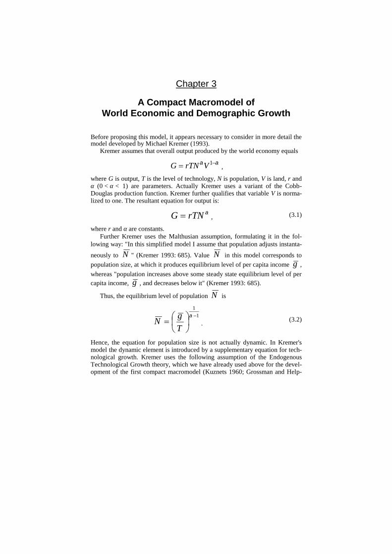
Before proposing this model, it appears necessary to consider in more detail themodel developed by Michael Kremer (1993).

Kremer assumes that overall output produced by the world economy equals

1VrTNG ,

where G is output, T is the level of technology, N is population, V is land, r andα (0 < α < 1) are parameters. Actually Kremer uses a variant of the Cobb-Douglas production function. Kremer further qualifies that variable V is norma-lized to one. The resultant equation for output is:

rTNG , (3.1)

where r and α are constants.Further Kremer uses the Malthusian assumption, formulating it in the fol-

lowing way: "In this simplified model I assume that population adjusts instanta-

neously to N " (Kremer 1993: 685). Value N in this model corresponds topopulation size, at which it produces equilibrium level of per capita income g ,whereas "population increases above some steady state equilibrium level of percapita income, g , and decreases below it" (Kremer 1993: 685).

Thus, the equilibrium level of population N is

11

T

gN . (3.2)

Hence, the equation for population size is not actually dynamic. In Kremer'smodel the dynamic element is introduced by a supplementary equation for tech-nological growth. Kremer uses the following assumption of the EndogenousTechnological Growth theory, which we have already used above for the devel-opment of the first compact macromodel (Kuznets 1960; Grossman and Help-

Macromodel of World Economic and Demographic Growth 35

man 1991; Aghion and Howitt 1992, 1998; Simon 1977, 1981, 2000; Komlosand Nefedov 2002; Jones 1995, 2003, 2005 etc.):"High population spurs technological change because it increases the numberof potential inventors…1. All else equal, each person's chance of inventingsomething is independent of population. Thus, in a larger population there willbe proportionally more people lucky or smart enough to come up with newideas" (Kremer 1993: 685); thus, "the growth rate of technology is proportion-al to total population" (Kremer 1993: 682).

(3.3)

Since this supposition was first proposed by Simon Kuznets (1960), we shalldenote the respective type of dynamics as "Kuznetsian"; and we shall denote as"Malthusian-Kuznetsian" those systems where "Kuznetsian" population-technological dynamics is combined with "Malthusian" demographics.

The Kuznetsian assumption is expressed mathematically by Kremer in thefollowing way:

bNTdt

dT: , (3.4)

where b is average innovating productivity per person.Note that this implies that the dynamics of absolute technological growth

rate can be described by the following equation:

bNTdt

dT . (3.5)

Kremer"Since population is limited by technology, the growth rate of population is proportionalto the growth rate of technology. Since the growth rate of technology is proportional tothe level of population, the growth rate of population must also be proportional to thelevel of population. To see this formally, take the logarithm of the population determina-tion equation, [(3.2)], and differentiate with respect to time:

):(1

1: Tdt

dTN

dt

dN

.

Substitute in the expression for the growth rate of technology from [(3.4)], to obtain

1 "This implication flows naturally from the nonrivalry of technology… The cost of inventing anew technology is independent of the number of people who use it. Thus, holding constant theshare of resources devoted to research, an increase in population leads to an increase in technolo-gical change" (Kremer 1993: 681).

Chapter 336

Nb

Ndt

dN

1: " (Kremer 1993: 686). (3.6)

Note that multiplying both parts of equation (3.6) by N we get

2aNdt

dN , (2.4')

where a equals

1b

a .

Of course, the same equation can be also written as

C

N

dt

dN 2

, (2.4)

where C equals

bC

1.

Thus, Kremer's model produces precisely the same dynamics as the ones of vonFoerster and Kapitza (and, consequently, it has just the same phenomenal fitwith the observed data). However, it also provides a very convincing explana-tion WHY throughout most of the human history the absolute world populationgrowth rate tended to be proportional to N2. Within both models the growth ofpopulation from, say, 10 million to 100 million will result in the growth ofdN/dt 100 times. However, von Foerster and Kapitza failed to explain convin-cingly why dN/dt tended to be proportional to N2. Kremer's model explains thisin what seems to us a rather convincing way (though Kremer himself does notappear to have spelled this out in a sufficiently clear way). The point is that thegrowth of the world population from 10 to 100 million implies that the humantechnology also grew approximately 10 times (as it turns out to be able to sup-port a ten times larger population). On the other hand, the growth of population10 times also implies 10-fold growth of the number of potential inventors, and,hence, 10-fold increase in the relative technological growth rate. Hence, the ab-solute technological growth will grow 10 x 10 = 100 times (in accordance toequation (3.5)). And as N tends to the technologically determined carrying ca-pacity ceiling, we have all grounds to expect that dN/dt will also grow just 100times.


Though Kremer's model provides a virtual explanation of how the WorldSystem's techno-economic development, in connection with demographic dy-namics, could lead to hyperbolic population growth, Kremer did not specify hismodel to such an extent that it could also describe the economic development ofthe World System and that such a description could be tested empirically.2 Nev-ertheless, it appears possible to propose a very simple mathematical model de-scribing both the demographic and economic development of the World Systemup to 1973 using the same assumptions as those employed by Kremer.

Kremer's analysis suggests the following relationship between per capitaGDP and population growth rate (see Diagram 3.1):

Diagram 3.1. Relationship between per capita GDPand Population Growth Rateaccording to Kremer (1993)

This suggests that in the lower range of per capita GDP the influence of this va-riable on the dynamics of population growth can be described with the follow-ing equation:

aSNdt

dN , (3.7)

where S is surplus, which is produced per person over the amount (m), which isminimally necessary to reproduce the population with a zero growth rate in aMalthusian system (thus, S = g – m, where g denotes per capita GDP).

2 In fact, such an operationalization did not make sense at the time when Kremer's article was sub-mitted for publication, as the long term empirical data on the world GDP dynamics were notsimply available at that moment.

A, population growth rate

g g, per capi-ta GDP

0

Chapter 338

Note that this model generates predictions that can be tested empirically. For

example, the model predicts that relative world population growth ( Ndt

dNrN : )

should be lineally proportional to the world per capita surplus production:

aSrN . (3.8)

The empirical test of this hypothesis has supported it. The respective correlationhas turned out to be in the predicted direction, very strong (R = 0.961), and sig-nificant beyond any doubt (p = 0.00004) (see Diagram 3.2):

Diagram 3.2. Correlation between the per capita surplus productionand world population growth rates for 1–1973 CE(scatterplot with fitted regression line)

Per capita surplus production (thousands of 1990 int.dollars,PPP)

321.5.4.3.2.1.05.04.03.02.01.005.004

.003.002

Ann

ual w

orld

pop

ulat

ion

grow

th r

ate

(%%

)

3

2

1

.5

.4

.3

.2

.1

.05

.04

.03

.02

.01

1950-1973

1913-19501870-1913

1820-18701700-1820

1600-1700

1500-1600

1000-1500

1-1000

NOTES: R = 0.961, p = 0.00004. Data source – Maddison 2001; Maddison's estimate of the worldper capita GDP for 1000 CE has been corrected on the basis of Meliantsev (1996: 55–97). S valueswere calculated on the basis of m estimated as 440 international 1990 dollars in purchasing powerparity (PPP); for the justification of this estimate see Korotayev, Malkov, and Khaltourina2005: 43–51.


The mechanisms of this relationship are perfectly evident. In the range $440–35003 the per capita GDP growth leads to very substantial improvements in nu-trition, health care, sanitation etc. resulting in a precipitous decline of deathrates (see, e.g., Diagram 3.3):

Diagram 3.3. Correlation between per capita GDP and death ratefor countries of the world in 1975

Per capita GDP (International 1990 dollars, PPP)

4000035000300002500020000150001000050000

De

ath

ra

te (

pe

r th

ou

san

d)

40

30

20

10

0

NOTE: data sources – Maddison 2001 (for per capita GDP), World Bank 2005 (for death rate).

For example, for 1960 the correlation between per capita GDP and death ratefor $440–3500 range reaches – 0.634 (p = 0.0000000001) (see Diagram 3.4):

3 Here and throughout the GDP is measured in 1990 international purchasing power parity dollarsafter Maddison (2001) if not stated otherwise.

Chapter 340

Diagram 3.4. Correlation between per capita GDP and death ratefor countries of the world in 1960 (for $440–3500 range)

GDP per capita (1990 international PPP dollars)

3500300025002000150010005000

De

ath

ra

te (

pe

r th

ou

san

d)

40

30

20

10

0

NOTE: R = – 0.634, p = 0.0000000001. Data sources – Maddison 2001 (for per capita GDP),World Bank 2005 (for death rate).

Note that during the earliest stages of demographic transition (correspondingjust to the range in question) the decline of the death rates is not accompaniedby a corresponding decline of the birth rates (e.g., Chesnais 1992); in fact, theycan even grow (see, e.g., Diagram 3.5).


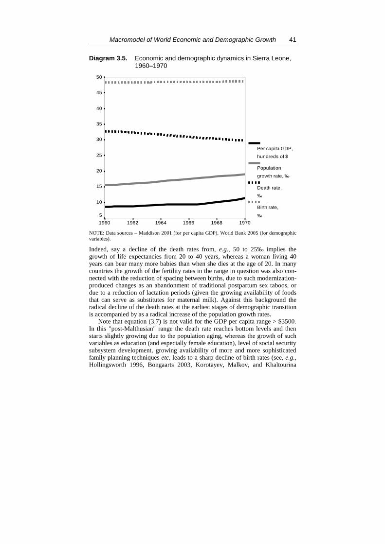
Diagram 3.5. Economic and demographic dynamics in Sierra Leone,1960–1970

197019681966196419621960

50

45

40

35

30

25

20

15

10

5

Per capita GDP,

hundreds of $

Population

growth rate, ‰

Death rate,

‰

Birth rate,

‰

NOTE: Data sources – Maddison 2001 (for per capita GDP), World Bank 2005 (for demographicvariables).

Indeed, say a decline of the death rates from, e.g., 50 to 25‰ implies thegrowth of life expectancies from 20 to 40 years, whereas a woman living 40years can bear many more babies than when she dies at the age of 20. In manycountries the growth of the fertility rates in the range in question was also con-nected with the reduction of spacing between births, due to such modernization-produced changes as an abandonment of traditional postpartum sex taboos, ordue to a reduction of lactation periods (given the growing availability of foodsthat can serve as substitutes for maternal milk). Against this background theradical decline of the death rates at the earliest stages of demographic transitionis accompanied by as a radical increase of the population growth rates.

Note that equation (3.7) is not valid for the GDP per capita range > $3500.In this "post-Malthusian" range the death rate reaches bottom levels and thenstarts slightly growing due to the population aging, whereas the growth of suchvariables as education (and especially female education), level of social securitysubsystem development, growing availability of more and more sophisticatedfamily planning techniques etc. leads to a sharp decline of birth rates (see, e.g.,Hollingsworth 1996, Bongaarts 2003, Korotayev, Malkov, and Khaltourina

Chapter 342

2005). As a result in this range the further growth of per capita GDP leads notto the increase of the population growth rates, but to their substantial decrease(see Diagram 3.6):

Diagram 3.6. Relationships between per capita GDP(1990 international PPP dollars, X-axis),Death Rates (‰, Y-axis), Birth Rates (‰, Y-axis),and Population Growth Rates4 (‰, Y-axis), nationswith per capita GDP > $3500, 1975,scatterplot with fitted Lowess lines

1450013500

1250011500

105009500

85007500

65005500

45003500

50

40

30

20

10

0

-10

Grow thrate, ‰

Birth

rate, ‰

Death

rate, ‰

NOTE: Data sources – Maddison 2001 (for per capita GDP), World Bank 2005 (for the other data).

4 Internal ("natural") population growth rate calculated as birth rate minus death rate. We used thisvariable instead of standard growth rate, as the latter takes into account the influence of emigra-tion and immigration processes, which notwithstanding all their importance are not relevant forthe subject of this chapter, because though they could affect in a most significant way the popula-tion growth rates of particular countries, they do not affect the world population growth.


This pattern is even more pronounced for the world countries of 2001, as be-tween 1975 and 2001 the number of countries that had moved out of the firstphase of demographic transition to the "post-Malthusian world" substantiallyincreased (see Diagram 3.7):

Diagram 3.7. Relationships between per capita GDP(2001 PPP USD, X-axis), Death Rates (‰, Y-axis),Birth Rates (‰, Y-axis), and Population GrowthRates (‰, Y-axis), nations with per capitaGDP > $3000, 2001, scatterplot with fitted Lowess lines

3600033000

3000027000

2400021000

1800015000

120009000

60003000

40

30

20

10

0

-10

Populationgrow th rate, ‰

Death rate,

‰

Birth rate,

‰

NOTE: Data source – World Bank 2005. Omitting the former Communist countries of Europe,which are characterized by a very specific pattern of demographic growth (or, in fact, to be moreexact, demographic decline – see, e.g., Korotayev, Malkov, and Khaltourina 2005: 302–29).

Chapter 344

It is also highly remarkable that as soon as the world per capita GDP (g) ap-proached $3000 and exceeded this (thus, with S ~ $2500), the positive correla-tion between S and r first dropped to zero (see Diagram 3.8); beyond S = 3300(g ~ 3700) it becomes strongly negative (see Diagram 3.9), whereas in the rangeof S > 4800 (g > 5200) this negative correlation becomes almost perfect (seeDiagram 3.10):

Diagram. 3.8. Correlation between the per capitasurplus production and world populationgrowth rates for the range $2400 < S < $3500(scatterplot with fitted regression line)


3.63.43.23.02.82.62.4

Ann

ual w

orld

pop

ulat

ion

grow

th r

ate

(%%

)

2.2

2.1

2.0

1.9

1972

1971

1970

1969

19681967

1966

1965

1964

1963

1962

NOTES: R = – 0.028, p = 0.936. Data source – Maddison 2001.


Diagram 3.9. Correlation between the per capita surplus productionand world population growth rates for S > $4800(scatterplot with fitted regression line)


5.95.65.35.04.74.44.13.83.53.2

Annual w

orld p

opula

tion g

row

th r

ate

(%

%)

2.2

2.0

1.8

1.6

1.4

1.2

1.0

NOTES: R = –0.946, p = 0.0000000000000003. Data sources – Maddison 2001 (for the world percapita GDP, 1970–1998 and the world population growth rates, 1970–1988); World Bank 2005(for the world per capita GDP, 1999–2002); United Nations 2005 (for the world population growthrates, 1989–2002).

Chapter 346

Diagram 3.10. Correlation between the per capita surplus productionand world population growth rates for S > $4800(scatterplot with fitted regression line)


5.85.65.45.25.04.8

Ann

ual w

orld

pop

ulat

ion

grow

th r

ate

(%%

)

1.5

1.4

1.3

1.2

1.1

20022001

2000

1999

1998

1997

19961995

1994

NOTES: R = –0.995, p = 0.00000004. Data sources – Maddison 2001 (for the world per capita GDP,1994–1998); World Bank 2005 (for the world per capita GDP, 1999–2002); United Nations 2005

(for the world population growth rates).

Thus, to describe the relationships between economic and demographic growthin the "post-Malthusian" GDP per capita range of > $3000, equation (3.7)should be modified, which is quite possible, but which goes beyond the scope ofthis chapter aimed at the description of economic and demographic macrody-namics of the "Malthusian" period of human history; this and will be done in thesubsequent chapters.

As was already noted by Kremer (1993: 694), in conjunction with equation(3.1) an equation of type (3.7) "in the absence of technological change [that is ifT = const] reduces to a purely Malthusian system, and produces behavior simi-lar to the logistic curve biologists use to describe animal populations facingfixed resources" (actually, we would add to Kremer's biologists those socialscientists who model pre-industrial demographic cycles – see, e.g., Usher 1989;


Chu and Lee 1994; Nefedov 2002, 2004; Malkov 2002, 2003, 2004; Malkovand Sergeev 2002, 2004; Malkov, Selunskaja, and Sergeev 2005; Turchin 2003;Korotayev, Malkov, and Khaltourina 2005).

Note that with a constant relative technological growth rate

( constTrT

T

.

) within this model (combining equations (3.1) and

(3.7)) we will have both constant relative population growth rate

( constNrN

N

.

, and thus the population will grow exponentially)

and constant S. Note also that the higher value of rT we take, the higher value ofconstant S we get.

Let us show this formally.Take the following system:

αgTNG (3.1)

aSNdt

dN (3.7)

cTdt

dT , (3.9)

where mN

GS .

Equation (3.9) evidently gives ct0eTT . Thus, αct

0 NegTG , and con-sequently

amNNeagTNmN

NegTa

dt

dN αct0

αct0

.

This is known as a Bernoulli differential equation: αyxgyxfdx

dy ,

which has the following solution:

dxxgeeα1Cey xFxFxFα1 ,

where dxxfα1xF , and C is constant.

In the case considered above, we have

Chapter 348

dteagTeeα1CeN ct0

tFtFtFα1 ,

where amt1αdtamα1tF .

So dteeeagTα1CeN ctamt1αamt1α0

amt1αα1

dteagTα1CeN tamα1c0

amtα1α1

tamα1c0amtα1α1 e

amα1c

agTα1CeN

This result causes the following equation for S:

m

eamα1c

agTα1C

egTmNegTm

N

NegTS

tamα1c0

tamα1c01αct

0

αct0

;

m

amα1c

aα1e

gT

C1

Stamα1c

0

.

Since 0c and 0α1 , it is clear that 0amα1c .

Consequently 0e tamα1c as t .

This means that m

aα1

amα1cS

t

, or finally

aα1

cS

, as t .

Note that coefficient c in equation (3.9) is nothing else but just the relativetechnological growth rate (rT = dT/dt : T). Thus within the system (3.1)-(3.7)-(3.9), with a constant relative technological growth rate (rT = c), the per capitasurplus (S) would also tend to some constant, and the higher value of relativetechnological growth rate (c = rT) we take, the higher value of constant S we getat the end.

This, of course, suggests that in the growing "Malthusian" systems S couldbe regarded as a rather sensitive indicator of the speed of technological growth.Indeed, within Malthusian systems in the absence of technological growth thedemographic growth will lead to S tending to 0, whereas a long-term systematicproduction of S will be only possible with systematic technological growth.5

5 It might make sense to stress that it is not coincidental that we are speaking here just about thelong-term perspective, as in a shorter-term perspective it would be necessary to take into accountthat within the actual Malthusian systems S was also produced quite regularly at the recovery


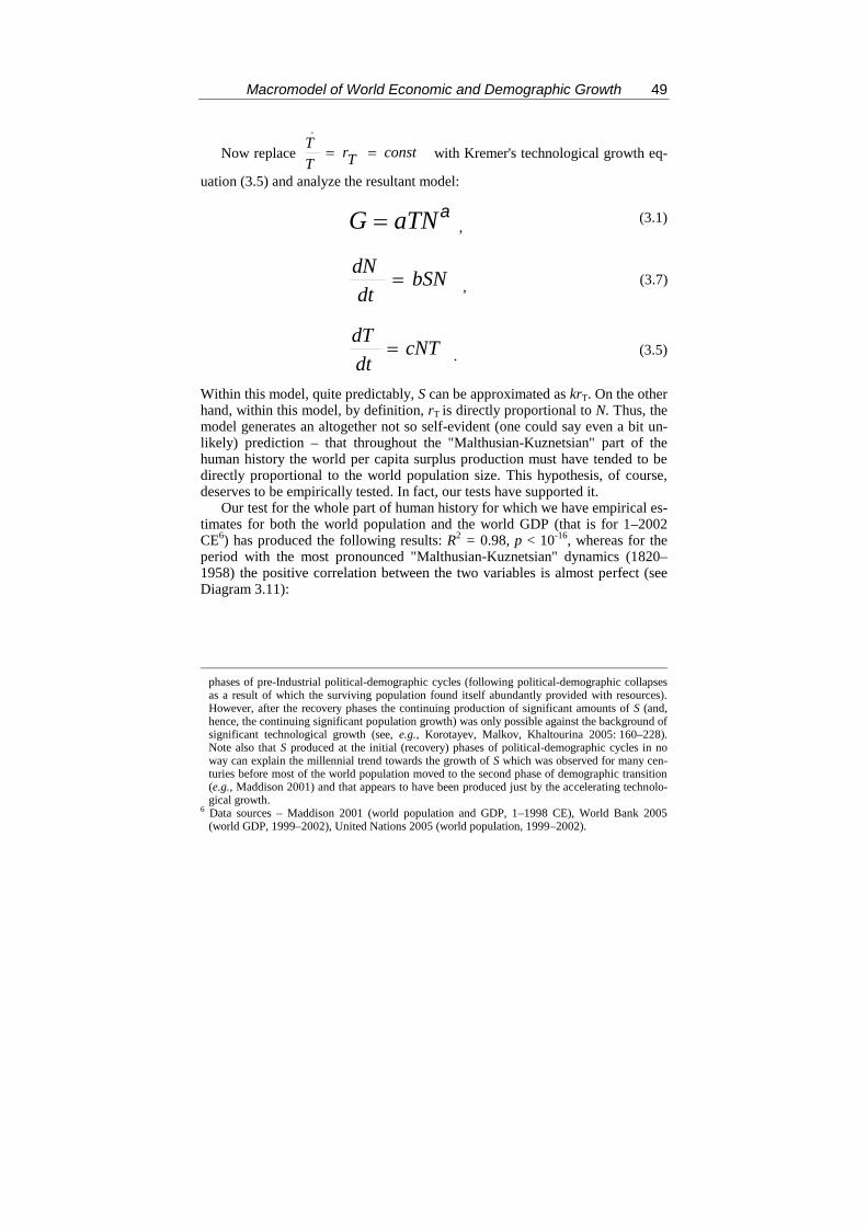
Now replace constTrT

T

.

with Kremer's technological growth eq-

uation (3.5) and analyze the resultant model:

aTNG ,(3.1)

bSNdt

dN , (3.7)

cNTdt

dT . (3.5)

Within this model, quite predictably, S can be approximated as krT. On the otherhand, within this model, by definition, rT is directly proportional to N. Thus, themodel generates an altogether not so self-evident (one could say even a bit un-likely) prediction – that throughout the "Malthusian-Kuznetsian" part of thehuman history the world per capita surplus production must have tended to bedirectly proportional to the world population size. This hypothesis, of course,deserves to be empirically tested. In fact, our tests have supported it.

Our test for the whole part of human history for which we have empirical es-timates for both the world population and the world GDP (that is for 1–2002CE6) has produced the following results: R2 = 0.98, p < 10-16, whereas for theperiod with the most pronounced "Malthusian-Kuznetsian" dynamics (1820–1958) the positive correlation between the two variables is almost perfect (seeDiagram 3.11):

phases of pre-Industrial political-demographic cycles (following political-demographic collapsesas a result of which the surviving population found itself abundantly provided with resources).However, after the recovery phases the continuing production of significant amounts of S (and,hence, the continuing significant population growth) was only possible against the background ofsignificant technological growth (see, e.g., Korotayev, Malkov, Khaltourina 2005: 160–228).Note also that S produced at the initial (recovery) phases of political-demographic cycles in noway can explain the millennial trend towards the growth of S which was observed for many cen-turies before most of the world population moved to the second phase of demographic transition(e.g., Maddison 2001) and that appears to have been produced just by the accelerating technolo-gical growth.

6 Data sources – Maddison 2001 (world population and GDP, 1–1998 CE), World Bank 2005(world GDP, 1999–2002), United Nations 2005 (world population, 1999–2002).

Chapter 350

Diagram 3.11. Correlation between world populationand per capita surplus production (1820–1958)

World Population (mlns.)

300027502500225020001750150012501000750

Wor

ld p

er C

apita

Sur

plus

Pro

duct

ion

(thou

sand

s of

$)

2.5

2.0

1.5

1.0

.5

0.0

NOTE: R2 > 0.996, p < 10-12.

Note that as within a Malthusian-Kuznetsian system S can be approximated askN, equation (3.7) may be approximated as dN/dt ~ k1N

2 (2.4'), or, of course, asdN/dt ~ N2 / C (2.4); thus, Kapitza's equation (2.4) turns out to be a by-productof the model under consideration.

Thus, we arrive at the following:

S ~ k1rT ,

rT = k2N .Hence,

dS/dt ~ krT /dt = k3dN/dt.

This implies that for the "Malthusian-Kuznetsian" part of human history dS/dtcan be approximates as k4dN/dt.

On the other hand, as dN/dt in the original model equals aSN, this, of course,suggests that for the respective part of the human history both the economic and


demographic World System dynamics may be approximated by the followingunlikely simple mathematical model:7

aSNdt

dN , (3.7)

bNSdt

dS , (3.10)

where N is the world population, and S is surplus, which is produced per personwith the given level of technology over the amount, which is minimally neces-sary to reproduce the population with a zero growth rate.

The world GDP is computed using the following equation:

SNmNG , (3.11)

where m denotes the amount of per capita GDP, which is minimally necessaryto reproduce the population with a zero growth rate, and S denotes "surplus"produced per capita over m at the given level of the world-system techno-economic development.

Note that this model does not contain any variables for which we do nothave empirical data (at least for 1–1973) and, thus, a full empirical test for thismodel turns out to be perfectly possible.8

Incidentally, this model implies that the absolute rate of the world popula-tion growth (dN/dt) should have been roughly proportional to the absolute rateof the increase in the world per capita surplus production (dS/dt), and, thus (as-suming the value of necessary product to be constant), to the absolute rate of theworld per capita GDP growth, with which dS/dt will be measured thereafter.Note that among other things this could help us to determine the proportion be-tween coefficients а and b.

Thus, if the model suggested by us has some correspondence to reality, onehas grounds to expect that in the "Malthusian-Kuznetsian" period of the humanhistory the absolute world population growth rate (dN/dt) was directly propor-tional to the absolute growth rate of the world per capita surplus production(dS/dt). The correlation between these two variables looks as follows (see Dia-gram 3.12):

7 Note that this model only describes the Malthusian-Kuznetsian World System in a dynamicallybalanced state (when the observed world population is in a balanced correspondence with the ob-served technological level). To describe the situations with N disproportionally low or high forthe given level of technology (and, hence, disproportionally high or low S) one would need, ofcourse, the unapproximated version of the model ((3.1) – (3.7) – (3.5)). Note, that in such casesN will either grow, or decline up to the dynamic equilibrium level, after which the developmentaltrajectory will follow the line described by the (3.7) – (3.10) model.

8 This refers particularly to the long-range data on the level of world technological development(T), which do not appear to be available now.

Chapter 352

Diagram 3.12. Correlation between World Average Annual AbsoluteGrowth Rate of Per Capita Surplus Production(S, 1990 PPP international dollars) and Average AnnualAbsolute World Population (N) Growth Rate(1 – 1973 CE), scatterplot in logarithmic scalewith a regression line

Average annual growth rate of S (1990 international $$)

10050

105

1.5

.1.05

.01.005

Ave

rag

e a

nn

ua

l gro

wth

ra

te o

f N

(m

lns.

) 100

50403020

10

5432

1

.5

.4

.3

.2

.1

.05.04.03

1950-1973

1913-19501870-1913

1820-18701700-1820

1600-1700

1500-1600

1000-1500

1-1000

NOTE: Data source – Maddison 2001; Maddison's estimates of the world per capita GDP for 1000CE has been corrected on the basis of Meliantsev (1996: 55–97).

Regression analysis of this dataset has given the following results (see Table3.1):


Table 3.1. Correlation between World Average Annual AbsoluteGrowth Rate of Per Capita Surplus Production (S, 1990PPP international dollars) and Average Annual AbsoluteWorld Population (N) Growth Rate (1 – 1950 CE),(regression analysis)



Model B Std. Error Beta(Constant) 0.820 0.935 0.876 0.414World Average An-nual Absolute GrowthRate of Per CapitaSurplus Production(1990 PPP internation-al dollars / year)

0.981 0.118 0.959 8.315 <0.001

Dependent variable: Average Annual Absolute World Population Growth Rate(mlns. / year)

R = 0.96, R2 = 0.92

Note that the constant in this case is very small within the data scale, statistical-ly insignificant, and lies within the standard error from 0, which makes it possi-ble to equate it with 0. In this case regression analysis gives the following re-sults (see Table 3.2):

Table 3.2. Correlation between World Average Annual AbsoluteGrowth Rate of Per Capita Surplus Production (S, 1990PPP international dollars) and Average Annual AbsoluteWorld Population (N) Growth Rate (1 – 1950 CE),(regression analysis, not including constant in equation)



Model B Std. Error BetaWorld Average An-nual Absolute GrowthRate of Per CapitaSurplus Production(1990 PPP interna-tional dollars / year)

1.04 0.095 0.972 10.94 <0.001

Dependent variable: Average Annual Absolute World Population Growth Rate(mlns. / year)

R = 0.97, R2 = 0.945

Chapter 354

Thus, just as implied by our second model, in the "Malthusian" period of humanhistory we do observe a strong linear relationship between the annual absoluteworld population growth rates (dN/dt) and the annual absolute growth rates ofper capita surplus production (dS/dt). This relationship can be described ma-thematically with the following equation:

dt

dS

dt

dN 04.1 ,

where N is the world population (in millions), and S is surplus (in 1990 PPP in-ternational dollars), which is produced per person with the given level of tech-nology over the amount, which is minimally necessary to reproduce the popula-tion with a zero growth rate.

Note that according to model (3.7, 3.10),

dt

dS

b

a

dt

dN .

Thus, it becomes possible to express coefficient b through coefficient a:

04.1b

a,

consequently:

aa

b 96.004.1 .

As a result, for the period under consideration it appears possible to simplify thesecond compact macromodel, leaving in it just one free coefficient:

aSNdt

dN , (3.7)

aNSdt

dS 96.0 , (3.12)

With our two-equation model we start the simulation in the year 1 CE and doannual iterations with difference equations derived from the differential ones:

Ni+1 = Ni + aSiNi ,Si+1 = Si + 0.96aNiSi .

The world GDP is calculated using equation (3.11).


We choose the following values of the constants and initial conditions in ac-cordance with historical estimates of Maddison (2001): N0 = 230.82 (in mil-lions); a = 0.000011383; S0 = 4.225 (in International 1990 PPP dollars).9

The outcome of the simulation, presented in Diagram 3.13 indicates that thecompact macromodel in question is actually capable of replicating quite reason-ably the world GDP estimates of Maddison (2001):

Diagram 3.13. Predicted and Observed Dynamicsof the World GDP Growth, in billions of 1990 PPPinternational dollars (1 – 1973 CE)

0

2000

4000

6000

8000

10000

12000

14000

16000

18000

0 500 1000 1500 2000

NOTE: The solid grey curve has been generated by the model; black markers correspond to the es-timates of world GDP by Maddison (2001).

9 The value of S0 was calculated with equation S = G/N – m on the basis of Maddison's (2001) es-timates for the year 1 CE. He estimates the world population in this year as 230.82 million, theworld GDP as $102.536 billion (in 1990 PPP international dollars), and hence, the world per ca-pita GDP production as $444.225 Maddison estimates the subsistence level per capita annualGDP production as $400 (2001: 260, 264). However, already by 1 CE most population of theworld lived in rather complex societies, where the population reproduction even at zero level stillrequired considerable production over subsistence level to maintain various infrastructures(transportation, legal, security, administrative and other subsystems etc.), without which even thesimple reproduction of complex societies is impossible almost by definition. Note that the fall ofper capita production in complex agrarian societies to subsistence level tended to lead to statebreakdowns and demographic collapses (see, e.g., Turchin 2003; Nefedov 2004; Malkov, Se-lunskaja, and Sergeev 2005; Korotayev, Malkov, and Khaltourina 2005). The per capita produc-tion to support the above mentioned infrastructures could hardly be lower than 10% of the subsis-tence level – that is close to Maddison's (2001: 259–60) estimates, which makes it possible to es-timate the value of m as $440, and hence, the value of S0 as $4.225.

Chapter 356

The correlation between the predicted and observed values for this simulationlooks as follows: R > 0.999; R2 = 0.9986; p << 0.0001. For the world popula-tion these characteristics are also very high: R = 0.996; R2 = 0.992;p << 0.0001.

According both to our model and the observed data up to the early 1970s wedeal with the hyperbolic growth of not only the world population (N), but alsoper capita surplus production (S) (see Diagram 3.14):

Diagram 3.14. Hyperbolic Growthof World Per Capita Surplus Production,in 1990 PPP international dollars(1 – 1973 CE)

0

500

1000

1500

2000

2500

3000

3500

0 500 1000 1500 2000


Note that even if S had not been growing, remaining constant, the world GDPwould have been growing hyperbolically anyway through the hyperbolic growthof the world population only. However, the hyperbolic growth of S observed


during this period of the human history led to the fact that the world populationcorrelated with the world GDP not lineally, but quadratically (see Diagram3.15):

Diagram 3.15. Correlation between World Populationand World GDP (1 – 1973 CE)

0

2000

4000

6000

8000

10000

12000

14000

16000

18000

0 1000 2000 3000 4000World Population (millions)

Wor

ld G

DP

(bill

ions

of 1

990

PPP

inte

rnat

iona

l dol

lars

)


Indeed, the regression analysis we have performed has shown here an almostperfect (R2 = 0.998) fit just with the quadratic model (see Diagram 3.16):

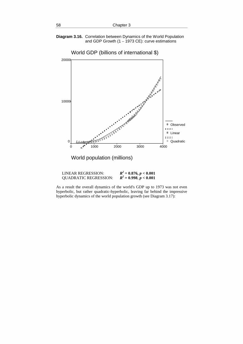
Chapter 358

Diagram 3.16. Correlation between Dynamics of the World Populationand GDP Growth (1 – 1973 CE): curve estimations

World GDP (billions of international $)

World population (millions)

40003000200010000

20000

10000

0

Observed

Linear

Quadratic

LINEAR REGRESSION: R2 = 0.876, p < 0.001QUADRATIC REGRESSION: R2 = 0.998, p < 0.001

As a result the overall dynamics of the world's GDP up to 1973 was not evenhyperbolic, but rather quadratic-hyperbolic, leaving far behind the impressivehyperbolic dynamics of the world population growth (see Diagram 3.17):


Diagram 3.17. The World GDP Growth from 1 CE up to the early 1970s(in billions of 1990 PPP international dollars)

0

2000

4000

6000

8000

10000

12000

14000

16000

0 500 1000 1500 2000


The world GDP growth dynamics would look especially impressive if we takeinto account the quite plausible estimates of this variable change before 1 CEproduced by DeLong (1998), see Diagram 3.18:

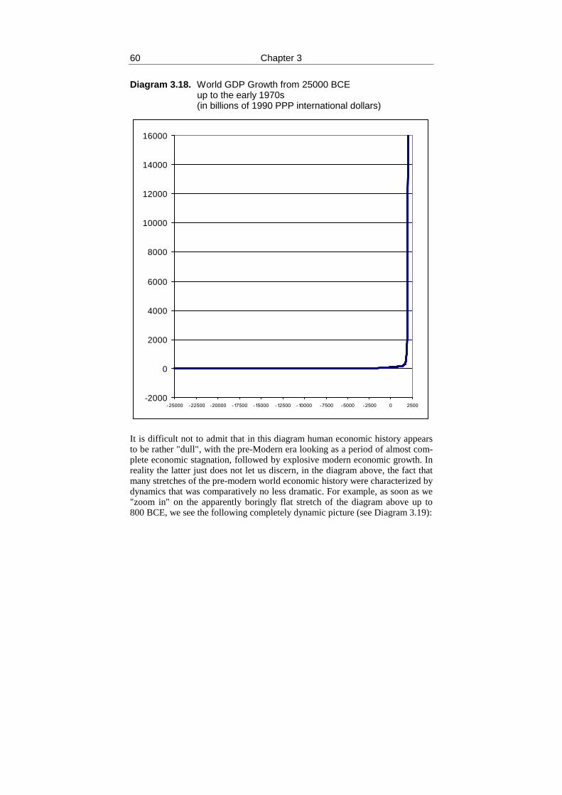
Chapter 360

Diagram 3.18. World GDP Growth from 25000 BCEup to the early 1970s(in billions of 1990 PPP international dollars)

-2000

0

2000

4000

6000

8000

10000

12000

14000

16000

-25000 -22500 -20000 -17500 -15000 -12500 -10000 -7500 -5000 -2500 0 2500

It is difficult not to admit that in this diagram human economic history appearsto be rather "dull", with the pre-Modern era looking as a period of almost com-plete economic stagnation, followed by explosive modern economic growth. Inreality the latter just does not let us discern, in the diagram above, the fact thatmany stretches of the pre-modern world economic history were characterized bydynamics that was comparatively no less dramatic. For example, as soon as we"zoom in" on the apparently boringly flat stretch of the diagram above up to800 BCE, we see the following completely dynamic picture (see Diagram 3.19):


Diagram 3.19. World GDP Growth from 25000 BCE up to 800 BCE(in billions of 1990 PPP international dollars)

0

5

10

15

20

25

30

35

-25500 -20500 -15500 -10500 -5500 -500

This, of course, is accounted for by the difference in scales. During the "ironrevolution" the World System economic growth was extremely fast in compari-son with all the earlier epochs; however, according to DeLong's estimates in ab-solute scale it constituted less than $10 billion a century. At present the worldGDP increases by $10 billion at average every three days (World Bank 2005).As a result, even the period of relatively fast World System economic growth inthe age of the "iron revolution" looks like an almost horizontal line in compari-son with the stretch of the modern economic growth. In other words the impres-sion of the pre-modern economic stagnation created by Diagram 3.18 could beregarded as an illusion (in the strictest sense of this word) produced just by thequadratic-hyperbolic trend of the world GDP growth up to 1973.

Chapter 362

We have already mentioned that, as has been shown by von Foerster, vonHoerner and Kapitza the world population growth before the 1970s is very wellapproximated by the following equation:

tt

CN

0. (2.1)

As according to the model under consideration S can be approximated as kN, itslong term dynamics can be approximated with the following equation:

tt

kCS

0. (3.13)

Hence, the long-term dynamics of the most dynamical part of the world GDP,SN, the world surplus product, can be approximated as follows:

20

2

)( tt

kCSN

. (3.14)

Note that if von Foerster, Mora, and Amiot had had at their disposal, in additionto the world population data, also the data on the world GDP dynamics for 1–1973 (published, however, only in 2001 by Maddison) they could have madeanother striking "prediction" – that on Saturday, 23 July, 2005 an "economicdoomsday" would take place; that is, on that day the world GDP would becomeinfinite. They would have also found that in 1–1973 CE the world GDP growthhad followed quadratic-hyperbolic rather than simple hyperbolic pattern.

Indeed, Maddison's estimates of the world GDP dynamics for 1–1973 CEare almost perfectly approximated by the following equation:

20 )(

Ctt

G

, (3.15)

where G is the world GDP, С = 17355487.3 and t0 = 2005.56 (see Diagram3.20):


Diagram 3.20. World GDP dynamics, 1–1973 CE(in billions of 1990 international dollars, PPP):the fit between predictions of quadratic-hyperbolicmodel and the observed data

200017501500125010007505002500

18000

16000

14000

12000

10000

8000

6000

4000

2000

0

predicted

observed

NOTE: R = 0.9993, R2 = 0.9986, p << 0.0001. The black markers correspond to Maddison's(2001) estimates (Maddison's estimates of the world per capita GDP for 1000 CE has been cor-rected on the basis of Meliantsev [1996: 55–97]). The grey solid line has been generated by the fol-

lowing equation:2)2006(

17749573.1t

G

. The best-fit values of parameters С (17749573.1) and t0

(2006) have been calculated with the least squares method (actually, as was mentioned above, thebest fit is achieved with С = 17355487.3 and t0 = 2005.56 [which gives just the "doomsday Satur-day, 23 July, 2005"], but we have decided to keep hereafter to the integer year numbers).

In fact, the fit provided by the simple hyperbolic model for the world GDP dy-namics for 1–1973 CE is also in no way bad, but still less perfect than the onefound for the quadratic hyperbolic model (see Diagram 3.21):

Chapter 364

Diagram 3.21. World GDP dynamics, 1–1973 CE(in billions of 1990 international dollars, PPP):the fit between predictions of hyperbolic modeland the observed data

200017501500125010007505002500

18000

16000

14000

12000

10000

8000

6000

4000

2000

0

predicted

observed

NOTE: R = 0.9978, R2 = 0.9956, p << 0.0001. The black markers correspond to Maddison's(2001) estimates (Maddison's estimates of the world per capita GDP for 1000 CE has been cor-rected on the basis of Meliantsev [1996: 55–97]). The grey solid line has been generated by the fol-

lowing equation:t

G

1987227906.1 . The best-fit values of parameters С (227906.1) and t0 (1987)

have been calculated with the least squares method.

This, of course, suggests that the long-term dynamics of the world GDP up tothe 1970s should be approximated better with a quadratic rather than simplehyperbola.

Note that, on the other hand, the simple hyperbolic model does fit the worldpopulation dynamics in 1–1973 much better than the world GDP one. Indeed,though the world 1–1973 CE GDP dynamics fits the simple hyperbolic modelof type (2.1) rather well (R = 0.9978, R2 = 0.9956, p << 0.0001), this fit is still


significantly worse than the one observed for the world population growth forthe same time (R = 0.9996, R2 = 0.9991, p << 0.0001) (see Diagram 3.22):

Diagram 3.22. World population dynamics, 1–1973 CE(in millions): the fit between predictionsof hyperbolic model and the observed data

200017501500125010007505002500

5000

4000

3000

2000

1000

0

predicted

observed

NOTE: R = 0.9996, R2 = 0.9991, p << 0.0001. The black markers correspond to Maddison's(2001) estimates. The grey solid line has been generated by the following equation:

tN

2014163158.78

. The best-fit values of parameters С (163158.78) and t0 (2014) have been cal-

culated with the least squares method.

However, the quadratic hyperbolic model renders a worse fit for the world pop-ulation (R = 0.9982, R2 = 0.9963, p << 0.0001) (see Diagram 3.23):

Chapter 366

Diagram 3.23. World population dynamics, 1–1973 CE (in millions):the fit between predictions of quadratic-hyperbolicmodel and the observed data

200017501500125010007505002500

5000

4000

3000

2000

1000

0

predicted

observed

NOTE: R = 0.9982, R2 = 0.9963, p << 0.0001. The black markers correspond to Maddison's(2001) estimates. The grey solid line has been generated by the following equation:

2)2065(33505220.7

tN

. The best-fit values of parameters С (33505220.702) and t0 (2065) have

been calculated with the least squares method.

Thus, up to the 1970s the hyperbolic growth of the world population was ac-companied by the quadratic-hyperbolic growth of the world GDP, just as issuggested by our model.

Chapter 4

A General Extended Macromodel ofWorld Economic, Cultural, and Demographic

Growth

One problem with the compact macromodels is that they do not account for thepost-1962 world population growth pattern. Take, for example, our simulationwith the first macromodel starting in 1650, which produced an almost perfect fitwith the observed data for 1650–1962. After 1962 (and especially after 1985)the gap between the predictions generated by the compact macromodel and ob-served values of the world population starts growing in a literally hyperbolicway (see Diagram 4.1):

Diagram 4.1. Growth of the Gap between Predictedand Observed Values, 1985–2003

20052000199519901985

Gap

bet

wee

n M

odel

Pre

dict

ions

and

Obs

erve

d Va

lues

(mln

s)

3000

2000

1000

0

Chapter 468

Our general extended macromodel of the world's economic, cultural, and demo-graphic growth is conceived to capture both of its two salient features: [1]hyperbolic growth trend in the pre-1962 era, and [2] increasing decline of theworld population growth rates afterwards.

Earlier researchers differ significantly in their analytical attempts to inte-grate into one model the model of hyperbolic growth and the model of globaldemographic transition. Kapitza (1992, 1999) connects the cause of the transi-tion with the limited nature of the characteristic times of the human develop-ment and the humankind development.1 Kremer (1993) considers the cause tobe the decline of fertility in wealthy families. There are also differences in thelevels of their approach: Kremer tries to describe the actual mechanism of tran-sition, whereas Kapitza does not look for the actual mechanism of fertility re-duction; he rather looks for the cause of the change of the regime in the globaldevelopment of humankind. Kapitza tries to explain why the current state is ex-ceptional, why the global demographic transition is taking place just now withina period of time that is microscopic on the historical scale, and just on the levelof development that has been achieved at the moment.

In the model suggested by us below we aim at accounting both for the transi-tion micromechanism and for the causes of the uniqueness of this phenomenon.The first thing which should be defined is the time period within which the re-spective model could claim to describe reality.

We have world population estimates starting from 1 million BP, and this isthe period for which the population growth is analyzed by Kapitza and Kremer.Despite all the attractiveness of such global theories, we will consciously re-strict the scale of our analysis. As in addition to population we use other indices(in particular the world GDP), the field of our model applicability is naturallyrestricted by the field of available statistical data. This does not mean that themodel is not applicable to earlier times, but in any case to corroborate this onewould need more data than is available at present.

More or less grounded estimates of the world GDP are available now for theperiod since 1 CE (Maddison 1995, 2001). Since 1950 they are known at a ra-ther high level of accuracy for every year (Maddison 2001; World Bank 2005).Thus our model only describes demographic and techno-economic growth from1 CE until the present. The prognostic potential of the model is also restrictedby time of the order of one century, which will be discussed specially below.

The uniqueness of the current sharp decrease of the world population growthrates consists in the fact that for the first time in the world history it is connectedwith the global decline of fertility rates. All the previous decreases took placebecause of increases in the rate of mortality due to famines, epidemics, warfareetc. In the framework of the global demographic process just this appears toconstitute the uniqueness of the present time, for which Kapitza tried to ac-

1 For more detail see Appendix 3.

General Extended Macromodel of the World System Growth 69

count. Indeed, in comparison with all the previous development of humankind,it is precisely our time that marks the transition to a new demographic regime.

Thus, the model involving the global demographic transition should detectfactors causing this transition, and first of all the factors of sharp fertility reduc-tion.

Kremer attempted to account for fertility decline through the introduction ofthe function of dependence of fertility on income (Diagram 3.1). However suchan explanation is not sufficient and rather indicates a mediated relationship.Thus, the drop in per capita incomes in the countries of the former Communistblock in the late 1980s and 1990s did not lead to sharp rise of fertility rates, asone would expect from Kremer's model; in fact we observe the exact reverse(see, e.g., Korotayev, Malkov, and Khaltourina 2005: 255–81). In addition tothis, the introduction of additional nonlinear functions including several para-meters, each of which is poorly measured in historical perspective, significantlydecreases the possibility to use the model for the description of actual data.

To determine the main factors and predictors of fertility reduction it makessense to address the empirical data. Analyses of large amounts of empirical datasuggest that one of the major factors of fertility reduction (in addition to, e.g.,the development of health care, or social security subsystems) is the growth ofeducation (especially, female education) (e.g., Hollingsworth 1996; McMichael2001; Bongaarts 2003 etc.).

The literacy rate (that is, the proportion of literate people in the adult popu-lation) turns out to be a good integral indicator of the education level. Note thatit has been shown that female literacy turns out to be a rather strong negativepredictor of fertility (e.g., Bongaarts 2003).

Our own cross-national test of fertility factors with stepwise multiple regres-sion has confirmed this conclusion (see Table 4.1):

Table 4.1. Regression Model of Fertility Factors in the World in 1995

ModelNonstadardized Coeffi-

cientsStandardizedCoefficient t p

B Standard Error βConstant 6.955 0.467 14.899 4 × 10-16

Female Literacy, % - 0.038 0.007 - 0.600 - 5.139 0.00001Number of Physi-

cians per 1000 - 0.253 0.117 - 0.239 - 2.155 0.036

Urbanization (% ofpopulation, leaving in

cities)- 0.006 0.007 - 0.087 - 0.866 0.391

NOTE: R = 0.837; R2 = 0.701; p = 2 × 10-11. DATA SOURCE: SPSS 2005.

This three-factor model accounts for more than 70% of all the variation of fer-tility rates in 1995. This multiple regression analysis confirms that female lite-

Chapter 470

racy is a major factor in fertility reduction in the course of modernization (let usnote here that – as we shall see below – female, male and overall literacy arevery strongly interconnected variables).

Our regression analysis of the World Bank (2005) and US Bureau of theCensus (2005) data on the female literacy and world population growth rateshas produced the following results (see Tables 4.2 and 4.3):

Table 4.2. World Population and Female Literacy, 1990–1999

Year World PopulationGrowth Rate (%)

World Literacy Rate,adult female (% of fe-

males, ages 15 andabove)

1990 1.58 61.611991 1.56 62.381992 1.49 63.131993 1.44 63.901994 1.43 64.661995 1.38 65.441996 1.37 66.561997 1.32 67.711998 1.29 68.601999 1.25 69.50

Table 4.3. Correlation between World Population Size andFemale Literacy, 1990–1999 (regression analysis)


Standardized Coef-ficients t Sig.

Model B Std.Error Beta

(Constant) 4.054 0.162 25.003 0.00000001Literacy rate,adult female (%of females, ages15 and above)

-0.04044 0.002 -0.985 -16.312 0.0000002


R = 0.971, R2 = 0.967

As we see, we do observe an extremely strong and significant correlation in thepredicted direction. In fact, this regression analysis suggests that 96.7% of allthe world macrodemographic variation in 1990–1999 is described by the fol-lowing equation:

r = 4.05 – 0.0404F,


where F is world female literacy (%), and r is the annual population growthrate (%).

Note that this model predicts that when the world population literacy be-comes 100% (which by definition implies 100% female literacy), the worldpopulation growth rate will be 0.01% (4.05 – 0.0404 × 100), which is extremelyclose to the one of the main assumptions of our model below.

Thus, there are definite grounds to consider literacy as a good integral indexof those modernization processes that could be considered as fertility reductionfactors. The fertility decline in connection with the growing literacy rate is freefrom the defects of Kremer's explanation connecting the declining fertility di-rectly with growing incomes. Our explanation has no problem with the abovecited case of the decreasing incomes not being accompanied by increasing fer-tility in the post-Communist countries (in the late 1980s and early 1990s). Onthe other hand, the suggested explanation is wider than Kremer's in the sensethat literate people tend to earn more than the illiterate ones. Thus, Kremer'sexplanation only works in the periods of stability, whereas our explanationworks both for stable and crisis periods.

We would like to stress that in no way are we going to claim that the literacygrowth is the only factor in the demographic transition. We do not deny impor-tant roles played by such factors as the development of medical care, or socialsecurity subsystems (e.g., Chesnais 1992). Note that these variables togetherwith literacy can be regarded as different parameters of one integrative varia-ble – the human capital development index (e.g., Denison 1962; Schultz 1963;Lucas 1988; Scholing and Timmermann 1988; Meliantsev 1996, 2003, 2004a,2004b). On the other hand, both of these variables display a very strong correla-tion with literacy.2 In general, if we know that in country A the proportion of li-terate population is 95%, and in country B this proportion is 25%, we can beperfectly sure that the health care and social security subsystems in country Aare about an order of magnitude more developed than in country B. Note alsothat the modern medical care development is connected in the most direct waywith the development of the education subsystem. The development and diffu-sion of new medical technologies (including, naturally, the family planningones) is very strongly connected with the development of education. E.g., the

2 For example, our cross-national analysis of World Development Indicators database for the year1975 shows that there is a strong and significant correlation between total literacy rate and thepercentage of birth attended by skilled personnel (R = 0,83; p < 0,0001, similar results were ob-tained for other years) (World Bank 2005). On the other hand, our analysis of the data for theyear 1995 indicates that literacy rate below 30% predicts with the maximum possible value(Gamma = 1.0) social security taxes being below 5% of current revenue, and literacy rate below75% predicts in the same way security taxes being below 15% of current revenue. We have alsofound that the number of physicians per 1,000 correlates exponentially with the total literacy ratefor the same year (R = 0.844) (In this case the data on literacy are from World95 database [SPSS2005]; the data on other parameters are from World Development Indicators Database [WorldBank 2005]).

Chapter 472

medical specialists are produced by the education system, the education facili-tates the spread of medical information (including the information on familyplanning means and practices), and so on.

Thus, literacy rate turns out to be a very strong predictor of the developmentof both medical care and social security subsystems.

Hence, literacy has turned out to be a rather sensitive indicator of humancapital development level, which has made it possible to avoid including itsother parameters as separate variables in our model.

Note that the overall adult literacy turns out to be an extremely strong pre-dictor of both male and female literacy (see Table 4.4):

Table 4.4. Correlations between World Overall, Female,and Male Literacy Rates, 1970–1999

Literacy rate,adult total (%of people ages15 and above)

Literacy rate,adult female (%of females ages15 and above)

Literacy rate,adult male (%of males ages15 and above)

Literacy rate,adult total (% ofpeople ages 15and above)

Pearson Correla-tion 0.99984 0.99977

Sig. (2-tailed) <<0.0001 <<0.0001N 30 30

Literacy rate,adult female (%of females ages 15and above)


Sig. (2-tailed) <<0.0001 <<0.0001N 30 30

Literacy rate,adult male (% ofmales ages 15 andabove)


Sig. (2-tailed) <<0.0001 <<0.0001N 30 30

Correlations of such a level could, of course, hardly be regarded as anything butextremely strong, even notwithstanding the fact that here we are dealing with anevident autocorrelation component. That is why, though the effects of male andfemale literacy on demographic dynamics are rather different, it has turned outto be possible to avoid including them as separate variables in model.

An important additional factor that led us to choose literacy rather than anyother fertility reducing parameter of the human capital development index isthat this seems to be the only such parameter for which it appears possible toobtain long-term global historical data.

As a result, in order to account for the global demographic transition, model(3.7)-(3.10) should be extended to take into account the development of humancapital level (measured through literacy rate) as a factor of fertility decrease. Asa result of this modification, model (3.7)-(3.10) looks as follows:


)1( LaNSdt

dN , (4.1)

bNSdtdS

, (3.10)

)1( LcLSdtdL

, (4.2)

where L is proportion of literate population and a, b, and c are constants. Theinfluence of world literacy on the global demographic transition is expressedthrough the addition to (3.7) of the multiplier (1 – L), which results in equation(4.1). Such a modification implies that the growth of literacy affects negativelyfertility rates even in the absence of any resource limitations. As regards the factthat the death rates also decline with modernization, equation (4.1) takes thisfact into account too, since the natural population growth rate (which tends tozero when the literacy approaches to 100%) is, by definition, the difference be-tween the fertility rate and the death rate.

The introduced additional equation for the literacy growth (4.2) has the fol-lowing sense: the literacy growth rate is proportional to the proportion of lite-rate people in the whole population L (potential teachers), to the proportion ofilliterate people in the whole population (1 – L) (potential pupils), and the pres-ence of surplus S, which can be used for educational purposes (in addition tothis, S is connected with the technological level T, including the level of educa-tional technologies that accelerate the spread of education). From the mathemat-ical point of view equation (4.2) is analogous to logistic equation (0.2), becausewithin equation (4.2) the saturation is achieved with literacy level L = 1, whe-reas S accounts for the speed with which the saturation level is reached.

Notwithstanding the fact that this modification of the model is generallyquite logical, its version (4.1) – (3.10) – (4.2) needs additional justification. Asit is evident that with the same logical conclusions on the dependence of popu-lation growth rate on the literacy rate (or, on the dependence of literacy growthrate on the growth rate of the number of potential teachers etc.) the same modelmay be presented as:

321 )1( LSaNdt

dN ,

54 SbNdtdS ,

876 )1( LScLdtdL

,

where φ1, φ2, φ3, φ4, φ5, φ6, φ7, φ8 are some positive values that are not neces-sarily equal to one.

Chapter 474

As regards coefficients φ1, φ2, φ4, φ5, the following suggests that they couldbe considered to be equal to one: in the area, which is removed from the zone ofthe second phase of the global demographic transition, such coefficients de-scribe satisfactorily the hyperbolic growth and fit the empirical data very well(see Chapter 3). As regards values of the other coefficients, they should be alsodetermined on the basis of empirical data.

It is easy to notice that if φ1 = φ6 = 1, φ2 = φ7, φ3 = φ8, through the dividingof the first equation by the third we arrive at the following equation:

LN

ca

dLdN .

Its solution defines the relationship between L and N in the following way:

ac

NL ,(4.3)

where λ is a constant.Let us test this hypothesis with historical data. Diagram 4.2 presents data on

the simultaneous growth of world literacy and world population in double loga-rithmic scale:

Diagram 4.2. World Literacy (%) and World Population (millions)

NOTE: Rectangles correspond to 1 and 1000 CE, for which we have large dispersions of estimates.Estimates of the world population are by Kremer (1993), Maddison (2001) and US Bureau of theCensus (2005). World literacy = proportion of literate adult population, calculated on the basis ofMeliantsev's (1996, 2003, 2004a, 2004b) estimates and UNESCO/World Bank (2005) data forpost-1970 period.


Within such a scale a straight line corresponds to a power-law dependence. Thediagram suggests that power-law dependence (4.3) fits the available data ratherwell.

Thus, the available data (see Diagram 4.2) suggest the validity of relation(4.3), and thus argue in favor of the statement that φ1 = φ6 = 1, φ2 = φ7, φ3 = φ8,which, in view of our earlier estimate of the power of φ2 as 1.0, may be writtenas: φ1 = φ6 = φ2 = φ7 = 1, φ3 = φ8. As regards the equality of φ3 to 1.0, whatsupports this is the good fit (see Diagrams 4.3–8) of the observed data with thevalues generated by model (4.1)-(3.10)-(4.2). Of course, a finer "tuning" of themodel using parameters φ1…8 could enhance the fit, however, due to the high er-ror margins for existing data such a "fine tuning" does not make much sense, aswe do not know for sure the exact coordinates of the points to which the solu-tion should be tuned. In any case, within such a general model one should striveto decrease the number of those parameters that do not enhance the solution at aqualitative level.

The results of computer simulation with (4.1)-(3.10)-(4.2) with parameters

a = 1.085∙10-5 ($ ∙ year)-1 ;b = 6.51 ∙10 -12 (person ∙ year)-1 ;с = 8.2∙10-6 ($ ∙ year)-1 ;m~ ("necessary product per person") = 420 $

and initial conditions for 1 CE:

N0 = 170000000;S0 = 17.47 $ ;L0 = 0.052 ,

where L is a dimensionless quantity (ranging from 0 to 1), sign $ corresponds to1995 international dollar (PPP), are displayed at Diagrams 4.3–8:

Chapter 476

Diagram 4.3. World Population Growth

Values generated by the model (solid line) for the world population describewell both the pre-1962 hyperbolic growth and the global demographic transitionby the present (the observed values are indicated with grey crosses). With re-gards to the future, the model suggests a scenario a bit different from the inter-mediate UN forecast (light grey markers). The model suggests that at the finalphases the global demographic tradition will proceed in a less smooth way thanis implied by the UN forecasts.

A smoother transition could be achieved through the introduction ofφ3 = φ8 ≠ 1; however, the UN forecast is just one of many possible forecaststhat rely on their own models. On the other hand, the available historical dataare not sufficiently exact to support the hypothesis φ3 = φ8 ≠ 1.

Naturally, with appearance of new data the model could be corrected.


Diagram 4.4. World GDP Growth

The world GDP grew even more steeply than the world population and can bedescribed mathematically with equation (3.11). Notwithstanding the fact thatGDP is not included explicitly in the system of equations, in this diagram therespective points are calculated on the basis of equations (3.10) and (4.1).

Finally, consider the diagram displaying the relationship between the worldliteracy growth dynamics generated by the model and the observed values of therespective variable (see Diagram 4.5):

Chapter 478

Diagram 4.5. World Literacy Growth (%%)

Diagrams in double logarithmic scale hide the visual component of hyperbolicgrowth and make the results more visible, though the deviations also look moresaliently in this scale (Diagrams 4.6–8):

Diagram 4.6. World Population Growth in Double Logarithmic Scale


Diagram 4.7. World GDP Growth in Double Logarithmic Scale

Diagram 4.8. World Literacy Growth in Double Logarithmic Scale

Chapter 480

While commenting on these diagrams, it appears necessary to note that, not-withstanding local deviations, model (4.1)-(3.10)-(4.2) describes quite well theavailable empirical data, though the model only includes three coefficients.What is more, through normalization it appears possible to reduce two of themto 1.0 – in this case the model will only include one coefficient that is equal tothe exponent in equation (4.3). Thus, notwithstanding the extreme simplicity ofthe model, it describes very successfully the joint dynamics of three major indi-cators of the global evolution of humankind.

Chapter 5

A Special Extended Macromodel ofWorld Economic, Cultural, and Demographic

Growth

In this model we make the following additional assumptions: (1) a literate popu-lation makes more technological innovations than an illiterate one. Consequent-ly, literacy growth leads to acceleration of technological development. (2) In theModern era the level of the World System's economic development is deter-mined first of all by the level of development of human capital, which, we be-lieve, can be roughly estimated by the world literacy level. These assumptionsin conjunction with the assumptions of the models presented above suggest thefollowing functional scheme of relationships between modeled subsystems (seeDiagram 5.1):

Diagram 5.1. Functional Scheme of Relationshipsbetween Model Subsystems+

→→→→→→→→↑ ↓

Technology/economy (S)

+→→→→→→→→→→→→→→→→→→→

↓←←←←←←←←←←←←←←← ↓

+ ↑ ↓↓ ↑

Population (N)↓ ↑ →→→→

+ ↓ ↑ + + ↑↓ ↑ ←←←←↓ ↑

Literacy (L)

↑↑

→→→→→→→→→→→→→→→→→→▬

→→↓ ↑ ↑ ↓

→→→→→→→→ ←←←+ ▬

Chapter 582

The relationships between these three subsystems are modeled using the follow-ing set of differential equations:

),1(

,

),1(

LcSLdtdL

bLNdtdS

LaSNdtdN

where L is the proportion of the literate population and a, b, and c are constants.This model generates dynamics shown in Diagram 5.2:

Diagram 5.2. Dynamics Generated by the Model

-0.2

0

0.2

0.4

0.6

0.8

1

1.2

1.4

1.6

1.8

2

0 200 400 600 800 1000 1200 1400 1600 1800 2000 2200

NOTE: thick grey curve – the world population counted as proportion from its size at stabilizationlevel; thin black curve – literacy; thick black curve – level of the World System techno-economicdevelopment (S) counted as proportion from its level at world population stabilization point.

Special Extended Macromodel of the World System Growth 83

With such a compact model we are able to reproduce rather well both thehyperbolic growth of world population before 1962/3, and the subsequent in-creasing slow down of world population growth rates.

With our three-equation model we start the simulation in 1875 and do an-nual iterations with difference equations derived from the differential ones. Wechoose the following values of the constants and initial conditions: N = 1325million; K = 1; L = 0.221; a = 0.008 (this corresponds to the initial annual popu-lation growth rate and equals the average annual population growth rate in1875–1900 CE according to Kremer's estimations [1993]); b = 0.00005;c = 0.007. The outcome of the simulation, presented in Diagram 5.3 indicatesthat irrespective of all its simplicity the model is actually capable of replicatingquite reasonably the population estimates of Kremer (1993), US Bureau of theCensus (2005) and other sources (Thomlinson 1975; Durand 1977; McEvedyand Jones 1978: 342–51; Biraben 1980; Haub 1995: 5; UN Population Division2005; World Bank 2005) in most of their characteristics and in terms of the im-portant turning points:

Diagram 5.3. Predicted and Observed Dynamics of World PopulationGrowth, in millions

0

1000

2000

3000

4000

5000

6000

7000

1850 1900 1950 2000 2050

NOTE: The solid grey curve has been generated by the model; black markers correspond to the es-timates of world population by Kremer (1993) for pre-1950 period, and the US Bureau of Censusworld population data for 1950–2003.

1 Based on Meliantsev's (1996, 2003, 2004a, 2004b) estimates.

Chapter 584

The correlation between the predicted and observed values for this simulationlooks as follows: R = 0.9989, R2 = 0.9978, p << 0.0001 (Diagram 5.4):

Diagram 5.4. World Population: Correlation between Predictedand Observed Values

Predicted

7000600050004000300020001000

Ob

se

rve

d7000

6000

5000

4000

3000

2000

1000

The correlation between predicted and observed values of world literacy alsoturns out to be rather high (see Diagram 5.5):

Special Extended Macromodel of the World System Growth 85

Diagram 5.5. World Literacy, Proportion of Literate Adult Population:Correlation between Predicted and Observed Values

World Literacy, Proportion of Literate Adult Population: Predicted

.9.8.7.6.5.4.3.2

Ob

serv

ed

.8

.7

.6

.5

.4

.3

.2

R = 0.997, R2 = 0.994, p << 0.0001

This dynamics has exact parallels in the real world – the world populationgrowth rates increased most rapidly when the world literacy was approaching50% (as both in the model and in reality, the stretch between 30% and 70% waspassed within just a few decades compared with millennia during which the first10% were passed), they achieved their highest levels when the world literacyrate was around 50%, and started decreasing with a progressively amplifying

Chapter 586

speed almost immediately after it grew over 50% (cp. Kremer 1993: 683; USCensus Bureau 2005; World Bank 2005).2

Of course, the special macromodel has a much narrower applicability thanthe general ones. For example, it does not work at all for the preliterate periodof human history, as, according to the special macromodel, zero literacy wouldcorrespond to a zero rate of techno-economic and demographic growth, whereasthis does not match the reality at all. On the other hand, the special macromodeldescribe rather well the modernization period, which appears to reflect the factthat the development of human capital became the most important factor ofeconomic development (see, e.g.: Meliantsev 1996; Dobrynin, Dyatlov, andKurganskij 1999; Denison 1962; Schultz 1963; Scholing and Timmermann1988; Lucas 1988 etc.). Note that, as we shall see below (see Chapter 7), the li-teracy level could serve as a rather sensitive indicator of the overall level ofhuman capital development. Note also that we have at our disposal some datasuggesting that the growth of literacy could serve in itself as a powerful factorof economic development; this will be discussed in the next chapter.

2 Thus, it turns out that the sets of 2–3 differential equations specified above account for up to99.78 per cent of all the variation in demographic, economic, and cultural macrodynamics of theworld in the last 2,000–25,000 years. In fact, in some sense the second part of our Introduction toSocial Macrodynamics (Secular Cycles and Millennial Trends) will be concerned with the re-maining 0.22–0.34% (As was indicated above, the simulation with compact macromodel 1started in 500 BCE [and run till 1962 CE] already gave a correlation with observed data as highas 0.9983 [R2 = 0.9966], whereas in the second part of our Introduction we will be dealing main-ly with the last two millennia of the world history). As we will see, to account for the remainingfraction of the variation is much more difficult, and we will only be able to start this process.What is more, the models will become more and more bulky, less and less elegant. However, inmany senses this remaining fraction of variation is much more interesting than 99.66–99.78% ofit, as without accounting for it we shall never be able to make any specific, concrete and exactpredictions.

Chapter 6

Reconsidering Weber:Literacy and the Spirit of Capitalism

In his classic The Protestant Ethic and the Spirit of Capitalism, Max Webersuggested that Protestantism stimulated the development of modern capitalismin Europe and North America. Weber disregarded the wide-spread explanationof economic success of Protestants in Europe in the Modern Age as a result oftheir religious minority position. He pointed out that Germen Catholics did notachieve the same results despite being a religious minority in many parts ofGermany.

Weber explained significant differences between Catholics and Protestantsin their social status and economic success through the different world viewsinherent in the doctrines of these two confessions. He suggested that a decisiverole was played by the formation of a special "spirit of capitalism", which in-cluded the devotion to one's business, the desire to increase one's wealth in anhonest way and so on. According to Weber, the spiritual basis of capitalism wasgrounded in the vulgarized versions of the theology of Calvinism and some oth-er Protestant sects. It was, above all, the belief in predestination and (in vulga-rized versions) in the possibility of obtaining the signs of whether one is predes-tined to salvation, via perfection in one's profession.

Many of Weber's followers tended to exaggerate the effect of religious eth-ics on the economic dynamics. Yet, Weber himself wrote:"… however, we have no intention whatever of maintaining such a foolish and doctri-naire thesis as that the spirit of capitalism… could have only arisen as the result of cer-tain effect of the Reformation, or even that capitalism as an economic system is a crea-tion of the Reformation." (Weber 1972: 109).

Yet, this doctrinaire thesis is still frequently attributed to Weber (see, e.g.,Maddison 2001: 45). At the same time Weber, to our opinion, showed quiteconvincingly that the processes of religious evolution can produce some inde-pendent effect on socioeconomic development. On the other hand, the specialextended macromodel considered above suggests another explanation for thecorrelation between the spread of Protestantism and some increase in economicdevelopment, which has been noted by Weber.

As has been mentioned earlier, human capital development has been sug-gested as one of the most important factors of economic growth, whereas educa-

Chapter 688

tion is considered to be one of the most important components of human capital(see, e.g., Schultz 1963, Denison 1962, Lucas 1988, Scholing and Timmermann1988 etc.). We tested our special macromodel in Chapter 5, and one of the as-sumptions of this model was a significant positive effect of literacy level oneconomic growth. The model based on this condition corresponded well withthe historical data on the demographic, economic, and educational dynamics ofthe World System. Consequently, this hypothesis has passed preliminarytesting. Let us test it again using cross-national data.

In the 20th century mass literacy spread around the globe, and nowadays dif-ferences in literacy levels between different countries tend to disappear. At thesame time, according to our hypothesis, the differences in economic develop-ments of various countries are rooted in the period of the beginning of moderni-zation era. Therefore, it seems reasonable to explore the connection betweensuch indicators as GDP per capita at present and the literacy level in the early19th century.1 For the data on these variables, as well as on GDP per capita inthe early 19th century, see Table 6.1:

Table 6.1. GDP per capita in the Countries and Regions of the Worldin 1800 (international $ 1980, PPP2), GDP per capita in 2000(international $ 1995, PPP) and % of literate population in 1800

Country/region GDP per capitain 2000 (interna-tional $ 1995, PPP)

GDP per capitain 1800 (interna-tional $ 1980, PPP)

% of lite-rate popula-tion in 1800

USA 31338.3 690 58Great Britain 22652.5 1030 55Germany 23912.6 790 55France 23225.2 750 38Israel 18894.5 (35)Japan 23828.1 420 33Italy 22874.8 670 30China 3547.4 500 20Mexico 8182.2 690 11Brazil 6780.7 580 8Russia 6643.6 488 8India 2229.3 440 5Indonesia 2807.3 425 5Egypt 3253.4 325 3Sub-Saharan Africa 1557.3 (1)

NOTE: The source of the data on GDP per capita and literacy rate in 1800 is Meliantsev 1996; onGDP per capita and the literacy rate in Russia in 1800 see Meliantsev 2003; on GDP per capita in

1 Since the indicators of educational level are strongly correlated with each other, the percentage ofliterate population seems to be a good integral indicator of the level of education for the earlymodernization period.

2 Purchasing power parity

Reconsidering Weber 89

the countries and regions of the world in 2000 see World Bank 2005. Our estimates are in paren-theses.

The data in Table 6.1 show that the level of economic wealth in the early 19th

century in various regions did not differ greatly enough to be considered theleading factor of economic differentiation between the regions later on. Thus,per capita GDP in Mexico was approximately equal to that in the USA. Howev-er, the literacy rates differed significantly.

The correlation between literacy rates in 1800 and per capita GDP in 2000is presented in Diagram 6.1:

Diagram 6.1. Scatterplot of Literacy Rates in 1800(% of literate people among the adult population)and per capita GDP Levels in 2000(international $ 1995, PPP)

0,0 10,0 20,0 30,0 40,0 50,0 60,0

Literacy rate in 1800, %

0

10000

20000

30000

40000

GD

P pe

r cap

ita in

200

0, U

SD, P

PP

USA

Germany

UK

France

Israel

JapanItaly

China

MexicoBrazil

Russia

India

IndonesiaEgypt

Africa

R Sq Linear = 0,86

NOTE: R = 0.93; R2 = 0.86; p = 0.0000003 (one-tailed).

Diagram 6.1 shows that there is a strong and definitely significant linear corre-lation between the literacy rate in 1800 and GDP per capita at present. R2 coef-ficient indicates that this correlation explains 86% of the entire data dispersion.

Chapter 690

Therefore, the hypothesis that the spread of literacy was one of the majorfactors of modern economic growth gains additional support. On the one hand,literate populations have many more opportunities to obtain and utilize theachievements of modernization than illiterate ones. On the other hand, literatepeople could be characterized by a greater innovative-activity level, which pro-vides opportunities for modernization, development, and economic growth.

Literacy does not simply facilitate the process of perceiving innovation byan individual. It also changes her or his cognition to a certain extent. This prob-lem was studied by Luria, Vygotsky, and Shemiakin, the famous Soviet psy-chologists, on the basis of the results of their fieldwork in Central Asia in the1930s. Their study shows that education has a fundamental effect on the forma-tion of cognitive processes (perception, memory, cognition). The researchersfound out that illiterate respondents, unlike literate ones, preferred concretenames for colors to abstract ones, and situative groupings of items to categoricalones (note that abstract thinking is based on category cognition). Furthermore,illiterate respondents could not solve syllogistic problems like the followingone – "Precious metals do not get rust. Gold is a precious metal. Can gold getrust or not?". These syllogistic problems did not make any sense to illiteraterespondents because they were out of the sphere of their practical experience.Literate respondents who had at least minimal formal education solved the sug-gested syllogistic problems easily (Luria 1974, 1976, 1982: 47–69).

Therefore, literate workers, soldiers, inventors and so on turn out to be moreeffective than illiterate ones not only due to their ability to read instructions,manuals, and textbooks, but also because of the developed skills of abstractthinking. Some additional support for this could be found in Weber's book it-self:

"The type of backward traditional form of labor is today very often exemplified bywomen workers, especially unmarried ones. An almost universal complaint of employersof girls, for instance German girls, is that they are almost entirely unable and unwillingto give up methods of work inherited or once learned in favor of more efficient ones, toadapt themselves to new methods, to learn and to concentrate their intelligence, or evento use it at all. Explanations of the possibility of making work easier, above all moreprofitable to themselves, generally encounter a complete lack of understanding. Increas-es of piece rates are without avail against the stone wall of habit. In general it is other-wise, and that is a point of no little importance from our view-point, only with girls hav-ing a specifically religious, especially a Pietistic, background" (Weber 1972: 75−6).

We believe that the above mentioned features of the behavior of German femaleworkers in the late 19th−early 20th centuries simply reflects a relatively low edu-cational level of German women from labor circles at that time. The spread offemale literacy in Germany, as elsewhere, lagged behind that of male literacy(see Chapter 7). In the early 20th century the majority of women could write andread only in the most developed parts of Germany (Meliantsev 1996). More ra-

Reconsidering Weber 91

tional behavior of German workers from Pietistic circles could be easily ex-plained by the special role of education in the lives of Protestants.

The ability to read was essential for Protestants (unlike Catholics) to per-form their religious duty − to read the Bible. The reading of Holy Scripture wasnot just unnecessary for Catholic laymen, for a long time it was even prohibitedfor them. The edict of the Toulouse Synod (1229) prohibited the Catholic lay-men from possessing copies of the Bible. Soon after that, a decision by the Tar-ragon Synod spread this prohibition to ecclesiastic people as well. In 1408, theOxford Synod absolutely prohibited translations of the Holy Scripture. From thevery beginning, Protestant groups did not accept this prohibition. Thus, Luthertranslated in 1522–1534 first the New Testament, and then the Old Testament,into German, so that any German-speaking person could read the Holy Scrip-ture in his or her native language. Moreover, the Protestants viewed reading theHoly Scripture as a religious duty of any Christian. As a result, the level of lite-racy and education was, in general, higher for Protestants not only than it wasfor Catholics and for followers of other confessions that did not provide reli-gious stimuli for learning literacy (see, for example: Malherbe 1997: 139–57).

In our opinion, this could explain to a considerable extent the differencesbetween economic performance of the Protestants and the Catholics in the late19th − early 20th centuries in Europe noticed by Weber. One of Weber's researchgoals was to show that religion can have independent influence on economicprocesses. The results of our study support this point. Indeed, spiritual leadersof Protestantism persuaded their followers to read the Bible not to support theeconomic growth but for religious reasons, which were formulated as a result ofideological processes that were rather independent of economic life. We do notquestion that specific features of Protestant ethics could have facilitated eco-nomic development. However, we believe that we found another (and probablymore powerful) channel of Protestantism's influence on the economic growth ofthe Western countries.

Chapter 7

Extended Macromodelsand Demographic Transition Mechanisms

To start with, the compact macromodels we discussed specify only the mostgeneral mechanisms of world population growth. However, we also need toknow how the macrotrends are produced on a more specific level. The popula-tion growth rate is a resultant of two determinant variables: fertility rate andmortality rate.1 What kind of dynamics of these two variables could produce theobserved demographic macrotrends?

The most evident more specific mechanism accounting for both the hyper-bolic population growth in 1850–1962/3 and the "inverse hyperbolic" trend af-terwards is the demographic transition itself (e.g., Chesnais 1992; Kapitza1999). As is well known, during the first phase of demographic transition a ra-ther sharp decline of mortality rates is observed. This is followed by decline infertility rates (through the introduction of family planning practices and tech-nologies as a proximate cause), but with a substantial time lag. As a result, forconsiderable periods of time we observe pronounced trends towards the rise ofthe population growth rates against the background of growing population.This, of course, produces just a hyperbolic effect – the higher is the population(N), the higher is the population growth rate (r). Since the 19th century more andmore populations of the world entered the demographic transition. Till the1960s the number of populations which entered the 2nd phase of the demograph-ic transition did not compensate for the hyperbolic growth of the 1st phase popu-lations; hence, the hyperbolic growth trend was characteristic not only for indi-vidual populations, but also for world population as a whole.

In fact, the demographic transition mechanism fits the compact macromodelrather well, specifying more concrete links between the variables in question.When the technology starts growing significantly faster than the population (inour simulation this process started in the 19th century and greatly accelerated inthe 20th century, which correlates well with the observed data), this results in asignificant growth of GDP per capita, and hence, per capita consumption, health

1 Of course, if we deal with population dynamics of individual countries we have also to take intoaccount emigration and immigration rates. However, as the two respective variables do not affectthe growth rate of the world population as a whole, we do not have to consider them on our levelof analysis.

Demographic Transition Mechanisms 93

status, and hence the decrease of mortality rates. With further growth of per ca-pita GDP we have more and more investment in spheres other than the subsis-tence economy, including education. On the one hand, the growth of educationfurther speeds up GDP growth through stimulating the increase of innovationrate, but on the other hand, it decreases fertility. In the compact macromodelthis time lag is simulated in the following way: until literacy level reaches 50%the effect of the increase of this parameter on the growth of S (and consequentlyN) is felt much more strongly than the inverse effect of L on N, which results inhyperbolic population growth. This has evident correlates in the real world:growth of a literate minority, say, from 5 to 30% (against the background of ra-pidly growing overall population) would mean a tremendous increase of a num-ber of potential effective innovators; what is more, due to the "nonrivalry oftechnology" effect discussed above, the innovations made by a literate minoritycan be used (and are used) by illiterate populations and for the benefit of illite-rate populations. In the meantime the negative influence of female literacy onbirth-rates (and, hence, the population growth rates) is still quite weak and doesnot counterweight the negative influence of the growing GDP per capita onmortality. Note that the growth of world literacy in this range did correlate withthe increase in the population growth rates (see Diagram 7.1):

Diagram 7.1. World Population Literacyand World Population Growth Rates, 1000–1950

0

0.2

0.4

0.6

0.8

1

1.2

1.4

1.6

1.8

2

1000 1150 1300 1450 1600 1750 1900

NOTES: grey curve – world population growth rates, % (Kremer 1993); black curve – world lite-racy, proportion of literate adult population, calculated on the basis of Meliantsev's (1996, 2003,2004a, 2004b) estimates. R = 0.961, R2 = 0.924, p < 0.01

Chapter 794

As we shall see below, a similar relationship can be detected by cross-nationalcomparisons for later periods. In the real world the mechanism specified aboveis further amplified by the fact that the growth of female literacy (which has thestrongest negative effect on fertility rates, and hence on population growthrates) lags significantly behind male literacy. This lag is still visible even for the1970–1999 period (see Diagram 7.2):

Diagram 7.2. World Male and Female Literacy,1970–1999 (World Bank 2005)

40

45

50

55

60

65

70

75

80

85

1970 1975 1980 1985 1990 1995

NOTES: grey curve – literacy rate, adult female (% of females ages 15 and above); black curve –literacy rate, adult male (% of males ages 15 and above).


In fact during this period, the growth of world literacy was accompanied by adecrease in the gap between the male and female literacy (see Diagram 7.3):

Diagram 7.3. World Overall Literacy and the Gap between Maleand Female Literacy, 1970–1999 (World Bank 2005)

10

20

30

40

50

60

70

80

1970 1975 1980 1985 1990 1995

NOTES: Black curve – literacy rate, adult total (% of people ages 15 and above); grey curve – gapbetween male literacy rate, adult female (% of females ages 15 and above).

However, in the 5–30% range the gap between male and female literacy tendedto grow (e.g., Meliantsev 1996, 2003, 2004a, 2004b). Note that this pattern canalso be detected through world-wide cross-national comparisons (see Diagram7.4):

Chapter 796

Diagram 7.4. Relationships between Overall Literacy (%, X-axis),Female Literacy (%, Y-axis), Male Literacy (%, Y-axis),Death Rates (‰, Y-axis), Birth Rates (‰, Y-axis),and Population Growth Rates2 (‰, Y-axis), nationswith overall adult literacy ≤ 30%, 1970 (World Bank2005), scatterplot with fitted Lowess lines

30252015105

60

50

40

30

20

10

0

Pop.Grow th Rate,‰

Female Literacy,%

Male Literacy,%

Death Rate,‰

Birth Rate,‰

As we see, this suggests that even after 1962/3, in the range of 5–30% overallliteracy, female literacy tended to grow much slower than the male literacy.Thus, in this range, economic growth (to a considerable extent supported by thegrowth of overall literacy [e.g., Meliantsev 1996, 2003, 2004a, 2004b]) leads toa rather rapid decline of mortality rates; however, the growth of female literacyin this range tends to be too slow to produce as strong a negative effect on the

2 Internal ("natural") population growth rate calculated as birth rate minus death rate. We used thisvariable instead of standard growth rate, as the latter takes into account the influence of emigra-tion and immigration processes, which notwithstanding all their importance are not relevant forthe subject of this chapter, because though they could affect in a most significant way the popula-tion growth rates of particular countries, they do not affect the world population growth.


fertility rates. As a result, the growth of literacy in this range is usually accom-panied by increase in population growth rates.

World Bank (2005) data suggest that world population growth rates starteddeclining systematically after overall world literacy reached c. 50% (by whichtime the male literacy had increased up to c. 60%, and female literacy toc. 40%). Thus, after L increases over 50% its inversed effect on N growth ratebecomes much stronger than the positive effect through S (which corresponds tothe second phase of demographic transition). Note that a similar pattern can alsobe observed in individual demographic histories of particular countries (see,e.g., Diagrams 7.5–6 below):

Diagram 7.5. Demographic and Literacy Dynamics in Ghana,1970–1997 (World Bank 2005)

19971995

19931991

19891987

19851983

19811979

19771975

19731971

1969

80

70

60

50

40

30

20

10

0

Overall Literacy,%

Male Literacy,%

Female Literacy,%


Death Rate,‰

Birth Rate,‰

Chapter 798

Diagram 7.6. Demographic and Literacy Dynamics in Iran,1970–2000 (World Bank 2005)

2000199019801970

90

80

70

60

50

40

30

20

10

0

Overall Literacy,%

Male Literacy,%

Female Literacy,%


Death Rate,‰

Birth Rate,‰

The inverse influence of above-50% literacy on population growth also can beeasily detected through a world-wide cross-national comparison (see Diagram7.7):


Diagram 7.7. Relationships between Overall Literacy (%, X-axis),Female Literacy (%, Y-axis), Male Literacy (%, Y-axis),Death Rates (‰, Y-axis), Birth Rates (‰, Y-axis),and Population Growth Rates (‰, Y-axis), nationswith overall adult literacy 50–90%, 1970 (World Bank2005), scatterplot with fitted Lowess lines

908580757065605550

100

90

80

70

60

50

40

30

20

10

0


Female Literacy,%

Male Literacy,%

Death Rate,‰

Birth Rate,‰

The demographic transition mechanism is usually illustrated with the followingdiagram (see Diagram 7.8):

Chapter 7100

Diagram 7.8. Demographic Transition Dynamics(from Kapitza 1999)

NOTES: dotted curve – birth rate; punctuated curve – death rate; solid curve –population growth rate.

Note that if we make a scatterplot of the type used above for the whole range,we will get death and birth rate curves that are quite similar to the ones found inthe standard diagrams of demographic transition (except perhaps for its extremeleft part, due to the fact that in world-wide databases for the late 20th century wehardly have any populations remaining in the very beginning of the demograph-ic transition process) (see Diagram 7.9):


Diagram 7.9. Relationships between Overall Literacy (%, X-axis),Death Rates (‰, Y-axis), Birth Rates (‰, Y-axis),1975 (World Bank 2005), scatterplotwith fitted Lowess lines

100806040200

60

50

40

30

20

10

0

Death rate,‰

Birth rate,‰

If we also plot curves for male and female literacy, we will see that they displayan almost perfect mirror image of demographic transition curves (see Diagram7.10):

Chapter 7102

Diagram 7.11. Relationships between Overall Literacy (%, X-axis),Female Literacy (%, Y-axis), Male Literacy (%, Y-axis),Death Rates (‰, Y-axis), and Birth Rates (‰, Y-axis),1975 (World Bank 2005),scatterplot with fitted Lowess lines

100806040200

100

80

60

40

20

0

Male Literacy,%

Female Literacy,%

Death rate,‰

Birth rate,‰

As we see in the left part of the diagram, the growing gap between male andfemale literacy is accompanied by the increasing gap between fertility and mor-tality (and, hence, increasing population growth rates), whereas in the right partof the diagram the decreasing gap between male and female literacy is accom-panied by the decreasing gap between fertility and mortality (and, hence, de-creasing population growth rates).

Note that, as has been shown above (see Chapter 4), overall adult literacyturns out to be an extremely strong predictor of both male and female literacy.Overall adult literacy turns out to be a highly sensitive and effective predictor of


general demographic dynamics within respective social macrosystems. Thegrowth of overall literacy in the 0–50% range (and especially, between 5 and30% range) would suggest rather strongly that we are dealing here with a situa-tion in which male literacy grows much faster than female literacy, and the neg-ative effect of overall literacy on the mortality rates3 is extremely unlikely to beoffset by the negative influence of female literacy on fertility rates. Hence, thegrowth of overall literacy in this range would tend to be accompanied by an in-crease in population growth rates.

On the other hand, the growth of overall adult literacy in the 50–100% range(and especially between 60 and 100%) predicts as strongly that we confronthere the situation in which female literacy grows significantly faster than maleliteracy, and the negative influence of female literacy on fertility far outweighsthe negative influence of overall literacy on mortality rates. Hence, the growthof the overall literacy in this range would tend to be accompanied by a quitesystematic decrease in population growth rates.

That is why, though the effects of male and female literacy on demographicdynamics are rather different, it has turned out to be possible to avoid includingthem as separate variables into our macromodels.

We would also like to stress again that in no way are we going to claim thatthe literacy growth is the only factor causing the demographic transition. Impor-tant roles were also played here by such factors as, for example, the develop-ment of medical care and social security subsystems. As was discussed above(see Chapter 4), these variables together with literacy can be regarded as differ-ent parameters of one integrative variable, the human capital development in-dex. These variables are connected with demographic dynamics in a way rathersimilar to the one detected above for literacy. At the beginning of the demo-graphic transition the development of the social security subsystem correlatesrather closely with the decline of mortality rates, as both are caused by essen-tially the same proximate factor – the GDP per capita growth. However, duringthe second phase, the social security development produces quite a strong inde-pendent effect on fertility rates through the elimination of one of the main in-centives for the maximization of the number of children in the family.

3 Of course, the proximate cause of declining mortality rates here is the growth of per capita GDP,which on the one hand leads to the elimination of such things as malnutrition, and on the other,stimulates the increase of investment in spheres other than the subsistence economy, many ofwhich (like, first of all, the medical care subsystem) also contribute to the decrease of mortality.At first glance, education looks like just one of such "GDP-per-capita-stimulated" spheres. Note,however, that here we are dealing with a truly dynamic ("hen-and-egg") relationship, when nei-ther variable x nor variable y could be justifiably identified as either purely dependent or purelyindependent. Yes, of course, the GDP-per-capita growth stimulates the development of educa-tion. But the education development also contributes in the most significant way to the GDP-per-capita growth (e.g., Meliantsev 1996, 2003, 2004a, 2004b). Note that this dynamic relationshipis explicitly reflected in the special extended macromodel.

Chapter 7104

The influence of the development of medical care on demographic dynamicsshows even closer parallels with the one produced by literacy growth. Note firstof all that the development of modern medical care is connected in the most di-rect way with the development of the education subsystem. On the other hand,during the first phase of the demographic transition the development of medicalcare acts as one of the most important factors in decreasing mortality. In themeantime, when the need to decrease fertility rates reaches critical levels, it isthe medical care subsystem that develops more and more effective family plan-ning technologies. It is remarkable that this need arises as a result of the de-crease in mortality rates, which could not reach critically low levels without themedical care subsystem being sufficiently developed. Hence, when the need todecrease fertility rates reaches critical levels, those in need almost by definitionfind the medical care subsystem sufficiently developed to satisfy this need quiterapidly and effectively.

Let us recollect that the pattern of literacy's impact on demographic dynam-ics has an almost identical shape: the maximum values of population growthrates cannot be reached without a certain level of economic development, whichcannot be achieved without literacy rates reaching substantial levels. Hence,again almost by definition the fact that the system reached the maximum levelof population growth rates implies that the literacy attained such a level that thenegative impact of female literacy on fertility rates would increase to such anextent that the population growth rates would start to decline. On the otherhand, the level of development of both medical care and social security subsys-tems displays a very strong correlation with literacy (see Chapter 4). Thus, lite-racy rate turns out to be a very strong predictor of the development of bothmedical care and social security subsystems.

Note that because, in reality as well as in our model, both the decline ofmortality at the beginning of demographic transition (causing a demographicexplosion) and the decline of fertility during its second phase (causing dramaticdecrease of population growth rates) were ultimately produced by essentiallythe same factor (human capital growth), there is therefore no need for us to in-clude mortality and fertility as separate variables in our model. On the otherhand, literacy has turned out to be a rather sensitive indicator of the level of thedevelopment of human capital, which has made it possible to avoid including itsother parameters as separate variables in extended macromodels.

Conclusion

Let us start the conclusion to the first part of our introduction to social macro-dynamics with one more brief consideration of the employment of mathematicalmodeling in physics.

The dynamics of every physical body is influenced by a huge number of fac-tors. Modern physics abundantly evidences this. Even if we consider such asimple case as a falling ball, we inevitably face such forces as gravitation, fric-tion, electromagnetic forces, forces caused by pressure, by radiation, by aniso-tropy of medium and so on.

All these forces do have some effect on the motion of the considered body.It is a physical fact. Consequently in order to describe this motion we shouldconstruct an equation involving all these factors. Only in this case may we"guarantee" the "right" description. Moreover, even such an equation would notbe quite "right", because we have not included those factors and forces whichactually exist but have not been discovered yet.

It is evident that such a puristic approach and rush for precision lead to ag-nosticism and nothing else. Fortunately, from the physical point of view, all theprocesses have their characteristic time scales and their application conditions.Even if there are a great number of significant factors we can sometimes neglectall of them except the most evident one.

There are two main cases for simplification:1. When a force caused by a selected factor is much stronger than all the

other forces.2. When a selected factor has a characteristic time scale which is adequate to

the scale of the considered process, while all the other factors have significantlydifferent time scales

The first case seems to be clear. As for the second, it is substantiated by theTikhonov theorem (1952). It states that if there is a system of three differentialequations, and if the first variable is changing very quickly, the second changesvery slowly, and the third is changing with an acceptable characteristic timescale, then we can discard the first and the second equations and pay attentiononly to the third one. In this case the first equation must be solved as an alge-braic equation (not as a differential one), and the second variable must be han-dled as a parameter.

Let us consider some extremely complicated process, for example, photo-synthesis. Within this process characteristic time scales (in seconds) are as fol-lows:

Conclusion106

1. Light absorption: ~ 0.000000000000001.2. Reaction of charge separation: ~ 0.000000000001.3. Electron transport: ~ 0.0000000001.4. Carbon fixation: ~ 1 – 10.5. Transport of nutrients: ~ 100 – 1000.6. Plant growth: ~ 10000 – 100000.

Such a spread in scales allows constructing rather simple and valid models foreach process without taking all the other processes into consideration. Eachtime scale has its own laws and is described by equations that are limited by thecorresponding conditions. If the system exceeds the limits of respective scale,its behavior will change, and the equations will also change. It is not a defect ofthe description – it is just a transition from one regime to another.

For example, solid bodies can be described perfectly by solid body modelsemploying respective equations and sets of laws of motion (e.g., the mechanicsof rigid bodies); but increasing the temperature will cause melting, and the samebody will be transformed into a liquid, which must be described by absolutelydifferent sets of laws (e.g., hydrodynamics). Finally, the same body could betransformed into a gas that obeys another set of laws (e.g., Boyle's law, etc.)

It may look like a mystification that the same body may obey different lawsand be described by different equations when temperature changes slightly (e.g.,from 95ºС to 105ºC)! But this is a fact. Moreover, from the microscopic pointof view, all these laws originate from microinteraction of molecules, which re-mains the same for solid bodies, liquids, and gases. But from the point of viewof macroprocesses, macrobehavior is different and the respective equations arealso different. So there is nothing abnormal in the dynamics of a complex sys-tem could have phase transitions and sudden changes of regimes.

For every change in physics there are always limitations that modify the lawof change in the neighborhood of some limit. Examples of such limitations areabsolute zero of temperature and velocity of light. If temperature is high enoughor, respectively, velocity is small, then classical laws work perfectly, but if tem-perature is close to absolute zero or velocity is close to the velocity of light, be-havior may change incredibly. Such effects as superconductivity or space-timedistortion may be observed.

As for demographic growth, there are a number of limitations, each of themhaving its characteristic scales and applicability conditions. Analyzing the sys-tem we can define some of these limitations.

Conclusion 107

Growth is limited by:

1. RESOURCE limitations:

1.1. Starvation – if there is no food (or other resources essential for vitalfunctions) there must be not growth, but collapse;time scale ~ 0.1 – 1 year;conditions: RESOURCE SHORTAGE.

This is a strong limitation and it works inevitably.

1.2. Technological – technology may support a limited number of work-ers;time scale ~ 10–100 years;conditions: TECHNOLOGY IS "LOWER" THAN POPULATION.

This is a relatively rapid process, which causes demographic cycles.

2. BIOLOGICAL

2.1. Birth rate – a woman cannot bear more than once a year;time scale ~ 1 year;condition: BIRTH RATE IS EXTREMELY HIGH.

This is a very strong limitation with a short time scale, so it will be the onlyrule of growth if for any possible reasons the respective condition (birth rate isextremely high) is observed.

2.2. Pubescence – a woman cannot produce children until she is mature;time scale ~ 15–20 years;conditions: EARLY CHILD-BEARING.

This condition is less strong than 2.1., but in fact condition 2.1. is rarely ob-served. For real demographic processes limitation 2.2. is more important than2.1. because in most pre-modern societies women started giving birth very soonafter puberty.

3. SOCIAL

3.1. Infant mortality – mortality obviously decreases population growth;time scale ~ 1–5 years;condition: LOW HEALTH PROTECTION.

Conclusion108

Short time scale; strong and actual limitation for pre-modern societies.

3.2. Mobility – in preagrarian nomadic societies woman cannot havemany children, because this reduces mobility;time scale: ~3 years;condition: NOMADIC HUNTER-GATHERER WAY OF LIFE.

3.3. Education – education increases the "cost" of individuals; it requiresmany years of education making high procreation undesirable. Highhuman cost allows an educated person to stand on his own economi-cally, even in old age, without the help of offspring. These limitationsreduce the birth rate;time scale: ~25–40 years;condition: HIGHLY DEVELOPED EDUCATION SUBSYSTEM.

All these limitations are objective. But each of them is ACTUAL (that is it mustbe included in equations) ONLY IF RESPECTIVE CONDITIONS AREOBSERVED.

If for any considered historical period several limitations are actual (undertheir conditions) then, neglecting the others, equations for this period must in-volve their implementation.

According to the Tikhonov theorem, the strongest factors are the ones hav-ing the shortest time scale. HOWEVER, factors with a longer time scale may"start working" under less severe requirements, making short-time-scale factorsnot actual, but POTENTIAL.

Let us observe and analyze the following epochs:

I. pre-agrarian societies;II. agrarian societies;III. post-agrarian societies.

We shall use the following notation:

– atypical – means that the properties of the epoch make the conditions practi-cally impossible;

– actual – means that such conditions are observed, so this limitation is actualand must be involved in implementation;

– potential – means that such conditions are not observed, but if some other li-mitations are removed, this limitation may become actual.

Conclusion 109

I. Pre-agrarian societies (limitation statuses):1.1. – ACTUAL1

1.2. – ACTUAL2

2.1. – potential2.2. – ACTUAL3.1. – ACTUAL3.2. – ACTUAL3.3. – atypical

II. Agrarian societies (limitation statuses):1.1. – ACTUAL1.2. – ACTUAL2.1. – potential2.2. – ACTUAL3.1. – ACTUAL3.2. – atypical3.3. – potential

III. Post-agrarian societies (limitation statuses):1.1. – atypical1.2. – potential/ACTUAL3

2.1. – potential2.2. – potential3.1. – atypical3.2. – atypical3.3. – ACTUAL

With our macromodels we only described agrarian and post-agrarian societies(due to the lack of some necessary data for pre-agrarian societies). According tothe Tikhonov theorem, to describe the DYNAMICS of the system we shouldtake the actual factor which has the LONGEST time-scale (it will represent dy-namics, while shorter scale factors will be involved as coefficients – solutionsof algebraic equations).

So epoch [II] is characterized by 1.2, and [III] by 3.3. ([III] also involves1.2, but for [III] resource limitation 1.2 is much less essential, because it con-

1 Systematic (not occasional short-term) starvation is caused by imbalance of technology and popu-lation, so 1.1. may be included in 1.2.

2 According to the Tikhonov theorem, we may neglect the oscillations of population (demographiccycles), because their time scales are at least 10 times shorter than the scale of the historical pe-riod which is taken into account.

3 Technology produces much more than is necessary for sustenance, but the growing living stan-dards also require more resources.

Conclusion110

cerns growing life standards, and not vitally important needs). Thus, the demo-graphic transition is a process of transition from II:[1.2] to III:[3.3].

Limitation 3.3 at [III] makes biological limitations unessential but potential(possibly, in the future, limitation 3.3 could be reduced, for example, throughthe reduction of education time due to the introduction of advanced educationaltechnologies, thereby making [2.2] actual again; possibly cloning might make[2.1] and [2.2] obsolete, so there would become apparent new limitations).

In conclusion, we want to note that hyperbolic growth is a feature whichcorresponds to II:[1.2]; there is no contradiction between hyperbolic growth it-self and [2.1] or [2.2]. Hyperbolic agrarian growth never does reach the birth-rate, which is close to conditions of [2.1]. If it was so, hyperbola will obviouslyconvert into an exponent, when birth-rate comes close to [2.1] (just as physicalvelocity may never exceed the velocity of light) – and it would not be a weak-ness of the model, just common sense. It would be just [1.2] → [2.1, 2.2].

But actual demographic transition [1.2] → [3.3] is more drastic than this[1.2] → [2.1, 2.2]! [3.3] is reducing the birth-rate much more actively, and itmay seem strange: the system WAS MUCH CLOSER TO [2.1] and [2.2]WHEN IT WAS GROWING SLOWER – during the epoch of [II]! (This is notnonsense, because slower growth was the reason of [2.1] and [3.1]).

As for the "after-doomsday dynamics", if there is no resource or spatial limi-tation (as well as [3.1]), then [2.1] and [2.2] will become actual. If they are alsoremoved (through cloning, etc.), then there will appear new limitations.

But if we consider the solution of C/(t0 – t) just formally, the after-doomsdaydynamics makes no sense. But this is "normal", just as temperature below abso-lute zero, or velocity above the velocity of light, makes no sense.

Thus, as we have seen, 99.3–99.78 per cent of all the variation in demo-graphic, economic and cultural macrodynamics of the world over the last twomillennia can be accounted for by very simple general models.

Actually, this could be regarded as a striking illustration of the fact wellknown in complexity studies – that chaotic dynamics at the microlevel can gen-erate highly deterministic macrolevel behavior (e.g., Chernavskij 2004).

As has already been mentioned in the Introduction, to describe the behaviorof a few dozen gas molecules in a closed vessel we need very complex mathe-matical models, which will still be unable to predict the long-run dynamics ofsuch a system due to an inevitable irreducible chaotic component. However, thebehavior of zillions of gas molecules can be described with extremely simplesets of equations, which are capable of predicting almost perfectly the macro-dynamics of all the basic parameters (and just because of chaotic behavior at themicrolevel).

Our analysis suggests that a similar set of regularities is observed in the hu-man world too. To predict the demographic behavior of a concrete family wewould need extremely complex mathematical models, which would still predicta very small fraction of actual variation due simply to inevitable irreducible

Conclusion 111

chaotic components. For systems including orders of magnitude higher numbersof people (cities, states, civilizations), we would need simpler mathematicalmodels having much higher predictive capacity. Against this background it ishardly surprising to find that the simplest regularities accounting for extremelylarge proportions of all the macrovariation can be found precisely for the largestpossible social system – the human world.

This, of course, suggests a novel approach to the formation of a generaltheory of social macroevolution. The approach prevalent in social evolutionismis based on the assumption that evolutionary regularities of simple systems aresignificantly simpler than the ones characteristic of complex systems. A ratherlogical outcome of this almost self-evident assumption is that one should firststudy the evolutionary regularities of simple systems and only after understand-ing them move to more complex ones.4 We believe this misguided approachhelped lead to an almost total disenchantment with the evolutionary approach inthe social sciences as a whole.5

4 A major exception here is constituted by the world-system approach (e.g., Braudel 1973; Wallers-tein 1974; Frank and Gills 1994; Chase-Dunn and Hall 1997; Chase-Dunn et al. 2003 etc.), butthe research of world-system theorists has up to now yielded rather limited results, to a signifi-cant extent, because they avoided the use of standard scientific methods and mostly remained onthe level of verbal constructions.

5 In fact, a similar fate would have stricken physicists if a few centuries ago they had decided thatthere is no real thing such as gas, that gas is a mental construction, and that one should start withsuch a "simple" thing as a mathematical model of a few free-floating molecules in a closed ves-sel.

Appendix 1

World Population Growth Forecast (2005–2050)

Of course, to use our Special Extended Macromodel for prediction of futurepopulation it is better to start the simulation as close to the period of time to bepredicted as possible.

Let us first check what kind of fit with observed data for the last decade ofthe 20th century we will have if we start the simulation with the compact ma-cromodel in 1990.1 The results look as follows (see Table A1.1):

Table A1.1. World Population, values predicted by the modeland observed values, 1991–2003

Year World Population, millionsPredicted by the Model Observed

1991 5368.18 5368.811992 5451.54 5452.991993 5534.74 5534.931994 5617.72 5615.481995 5700.46 5696.261996 5782.92 5775.521997 5865.05 5855.071998 5946.83 5933.091999 6028.22 6009.952000 6109.17 6085.482001 6189.67 6159.702002 6269.67 6232.702003 6349.12 6305.14R > 0.999, p << 0.0001

For the correlation between predicted and observed values of the world literacy(for 1991–1999) R = 0.995, R2 = 0.990, p << 0.0001.

1 N0 (5284.679, in millions) and L0 (0.696) correspond to the US Census Bureau (2005) and WorldBank (2005) estimates for 1990. S0 is taken as 1. Values of a (0.05197) and c (0.02978) are esti-mated on the basis of US Census Bureau (2005) and World Bank (2005) data on the growth ofworld population and literacy in respective year. The value of b is assumed as 0.000001.

World Population Growth Forecast (2005–2050) 113

Let us start now annual iterations in year 1999.2 This simulation predicts thefollowing future dynamics of the variables in question.

The model predicts the following dynamics of literacy for 2005 – 2050 (seeTable A1.2 and Diagram A1.1):

Table A1.2. Future World Population Literacy, 2010–2150

Year 2010 2020 2030 2040 2050 2060 2070Literacy 0.837 0.889 0.928 0.956 0.974 0.985 0.992Year 2080 2090 2100 2110 2120 2130 2150Literacy 0.996 0.998 0.999 0.9995 0.9998 0.9999 0.99998

Diagram A1.1. Predicted World Literacy Dynamics

0.7

0.8

0.9

1

1995 2005 2015 2025 2035 2045

2 N0 (6010, in millions) and L0 (0.7633) correspond to the US Census Bureau (2005) and WorldBank (2005) estimates for 1999. S0 is taken as 1. Values of a (0.05281) and c (0.04079) are esti-mated on the basis of US Census Bureau (2005) and World Bank (2005) data on the growth ofworld population and literacy in 1998. The value of b is assumed as 0.000001.

Appendix 1114

The model suggests that by 2050 97.4% of the world population will be literate,whereas by 2070 less than 1% of all the world population will remain illiterate.

The world population forecast generated by the model looks as follows (seeTable A1.3 and Diagram A1.2):

Table A1.3. World Population, 2010–2150, millions

Year 2010 2020 2030 2040 2050 2060 2070Population 6771.2 7324.6 7741.9 8037.3 8234.3 8358.7 8433.3Year 2080 2090 2100 2110 2120 2130 2150Population 8476.0 8499.4 8511.7 8517.8 8520.8 8522.2 8523.1

Diagram A1.2. World Population, 2010–2150, millions

5500

6000

6500

7000

7500

8000

8500

1995 2005 2015 2025 2035 2045

Thus, the model suggests that by 2050 the world's population will reach about8200 million, whereas by 2100 it will more or less stabilize at c. 8500 million.

Appendix 2

World Population Growth Rates andFemale Literacy in the 1990s:

Some Observations

Our regression analysis of the World Bank (2005) and US Bureau of the Census(2005) data on the female literacy and world population growth rates has pro-duced the following results (see Tables A2.1–2):

Table A2.1. World Population and Female Literacy, 1990–1999

Year World PopulationGrowth Rate (%)

World Literacy Rate,adult female (% of fe-

males, ages 15 andabove)

1990 1.58 61.611991 1.56 62.381992 1.49 63.131993 1.44 63.901994 1.43 64.661995 1.38 65.441996 1.37 66.561997 1.32 67.711998 1.29 68.601999 1.25 69.50

Appendix 2116

Table A2.2. Correlation between World Population Growth Rateand Female Literacy, 1990–1999(regression analysis)


StandardizedCoefficients

t Sig.Model B Std.

Error Beta

4

(Constant) 4.054 0.162 25.003 0.00000001

Literacyrate, adultfemale (% offemales, ages15 andabove)

-0.04044 0.002 -0.985 -160.312 0.0000002

Dependent Variable: World Population Annual Growth Rate (%)R = 0.971, R2 = 0.967

As we see, we do observe an extremely strong and significant correlation in thepredicted direction. Indeed, this regression analysis suggests that 96.7% of allthe world macrodemographic variation in 1990–1999 is predicted by the fol-lowing equation:

r = 4.05 – 0.04044F, (A2.1)

where F is the world female literacy (%), and r is the annual population growthrate (%).

Note that this model predicts that when the world population's literacy be-comes 100% (which by definition implies 100% female literacy), the worldpopulation's growth rate will be 0.01% (4.054 – 0.04044 × 100), which is ex-tremely close to the one of the main assumptions of our compact macromodel.

On the other hand, our regression analysis of data on the female literacy andworld population size for the same period has produced the following results(see Table A2.3):

World Population Growth Rates and Female Literacy 117

Table A2.3. Correlation between World Population Size andFemale Literacy, 1990–1999 (regression analysis)


StandardizedCoefficients

t Sig.Model B Std.

Error Beta

(Constant) 3.235 1.901 1.701 0.127

World Popu-lation (bil-lions)

10.988 0.336 0.996 320.693 0.000000001

Dependent Variable: Literacy rate, adult female(% of females, ages 15 and above)

R = 0.996, R2 = 0.993

This suggests the following relationship between world population and femaleliteracy in the 1990s, a relationship quite congruent with the predictions of thecompact macromodel for the same phase:

F = 3.2 + 11N , (A2.2)

where N is the world population in billions, and F is the world female literacy(%).

Note that by substituting F in equation (A2.1) with the expression above(A2.2) we arrive at the following results:

r = 4.054 – 0.04044F = 4.054 – 0.04044(3.235 + 11N) =4.054 – 0.04044 × 3.235 – 0.04044 × 11N = 4.054 – 0.1308234 – 0.44484N =3.92 – 0.44N .

Thus, we arrive at the equation r = 3.92 – 0.44N, which is virtually identicalwith the one (r = 3.9 – 0.44N) produced above by the straightforward regres-sion analysis of world population size and world population growth rates for1990–2003 (1.1). Hence, for the 1990s the dynamic relationship between fe-male literacy, world population size, and world population growth rate appearsto produce exactly that very "inverse hyperbolic" world population growth pat-tern which we identified for this period at the beginning of this book.

Appendix 3

Hyperbolic Growth of the World Populationand Kapitza's model

The most fundamental research in the field of global demography that describesglobal demographic processes as a response of endogenous population kineticsbelongs to Kapitza (1992, 1999). That is, while von Foerster et al. (1960)pleaded for human beings to take matter into their own hands and reduce fertili-ty, Kapitza argued for population transitions that would stem from internal pop-ulation dynamics.

Kapitza's model differs from demographic models based on biological as-sumptions and maintaining that population growth is proportional to the popula-tion itself, which implies that mortality and fertility do not change significantlyin time:

aNdtdN , (A3.1)

where a is a constant. Instead Kapitza follows von Foerster et al. (1960) to sug-gest using the quadratic relationship to describe the population growth rate:

CN

dtdN 2

, (2.4)

where C is a constant.Equations of type (2.4) have been studied rather thoroughly (Kurdjumov

1999) and their solutions are known as "blow-up regimes". A characteristic fea-ture of such equations is that at a given finite moment of time t0 their solutionsgo to the infinity.

As regards equation (2.4) itself, the empirically found formula (2.1)

ttCN

0

(2.1)

Kapitza's Model 119

(where t0 depends on initial conditions) turns out to be just its solution.Indeed, take equation (2.4)

CN

dtdN 2

, (2.4)

where C is a constant.Separate the variables (that is, move everything containing N to one side of

the equation, everything containing t to the other) to get:

Cdt

NdN2

Through integration get:

constCdt

NdN

2

As is known,

11)1( nn x

nxdx

if 1n

(in fact this is a particular case for the following rule

1)1( nn xndxx for negative n not equal to –1,

which is inverse to the following differentiation rule 1 nn nxx ).

Thus,

constCt

N

1,

Appendix 3120

hence,

Cconstt

CN

.

The integration constant depends on initial conditions.For the sake of convenience it can be expressed in the following way:

0Ctconst ,

where t0 is the same constant, but multiplied by – C.Then the equation for N will be as follows:

ttCN

0

, (2.1)

where t0 is a constant dependent on the initial conditions.Thus, equation (2.4) describes satisfactorily the empirically found relation-

ship (2.1), and can be used as a model of the respective demographic process.However, though the interpretation of exponential equation (A3.1) is rather

transparent and stems from the averaging-out of biological processes, thehyperbolic growth described by equation (2.4) needs explanation and justifica-tion.

Kapitza considers as the cause of the quadratic relationship between theworld population size and the world population growth rate the fact that hu-mankind constituted a single system within which one could observe paired in-teractions involving information exchange, whereas the growth rates of separateparts depend significantly on the overall size of the system. According to Kapit-za, these are just the information interactions that constitute the main mechan-ism distinguishing humans from those animals among whom population growthis characterized by regularities expressed by equation (A3.1).

This way Kapitza accounts for the hyperbolic growth of world population upto 1962. As regards the solution of the second puzzle (a dramatic slow-down ofthe world population growth rates in the post-1963 era), Kapitza modifies hismodel in the following way.

As according to equation (2.4) the world population growth rate depends en-tirely on the population size and does not depend on any external conditions and

Kapitza's Model 121

resource limitations, the logic suggests that we look for the cause of the worlddemographic transition within the population itself, because for millennia no re-source limitations were capable, in the final analysis, of stopping the hyperbolicgrowth of the world population; whereas in the present-day world, demographictransition is not caused by resource limitations, as can be seen by the fact thatthe dramatic decline in the relative annual world population growth rates in therecent decades has taken place against the background of growing GDP per ca-pita. Kapitza considers as an especially important parameter what he calls "thecharacteristic human life-span" (τ = 42 years), determined by "internal extremecapability of the human system and the human to develop".

This parameter appears in various statistical estimations; in particular Kapit-za notes that the demographic transition takes place within a characteristic pe-riod of time, which equals doubled τ.

If we place in the quadratic growth equation (2.4) its solution (2.1), it can beexpressed as follows:

20 )( tt

CdtdN

. (A3.2)

To account for the demographic transition Kapitza introduces into this equationparameter τ:

220 )(

ttC

dtdN

. (A3.3)

This equation does not produce a blow-up regime (when the solution goes upreaching infinity within a finite period of time); what is more, with this modifi-cation the world population stabilizes at the level of 10–12 billion, which cor-responds not badly to the estimations of the demographers.

In addition to this, equation (A3.3) makes it possible to derive an analyticalformula for the calculation of world population:

ttarcctgCN 1

, (A3.4)

Appendix 3122

where t1 is a parameter, which equals 2000 CE (which, according to Kapitza,corresponds to the middle point of the second phase of the world demographictransition).

The research conducted by Kapitza has shown in a quite convincing waythat the world population growth can be described mathematically without theintroduction of any additional variables, that is actually without taking any addi-tional factors into account. This effect creates Kapitza's grounds for proclaiminga "demographic imperative", that is the recognition of the primary and self-sufficient role of demography in the history of the development of human socie-ty.

However, neither Kapitza's basic equation (2.4) nor its modification (A3.3)describing the global demographic transition explains the mechanisms of the re-spective regularities; and on the phenomenological level, they remain mere as-sertions of empirically discovered regularities. The elegance of the "demo-graphic imperative" makes such an approach rather attractive; in the meantime,it somehow mystifies the results obtained. What is more, from the mathematicalpoint of view demographic data are products of the realization of some process,some integral curve, and from the mathematical point of view equations

CN

dtdN 2

and ttCN

0

are equivalent, as one is nothing else but a differential form of the other.However, notwithstanding their mathematical equivalence, the difference in

the form of their expression dictates a difference in their interpretation. Thus, aswas noted above, if equation (2.4), that includes just one variable N, createspreconditions for the declaration of a "demographic imperative", equation (2.1)turns out to be a departure point for eschatological conclusions formulated mostevidently (though, of course, quite ironically) in the title of the first article tobring the attention of the academic community to the fact of the hyperbolicgrowth of world population – "Doomsday: Friday, 13th November, 2026" (vonFoerster, Mora, and Amiot 1960). This suggests another thesis – the evolutionof humankind is connected not with the fundamental role of demography, butwith a fixed point in time, which is present in equation (2.1) as t0. In order toemphasize the role of temporal singularity the same equation can be written inan equivalent form:

20 )( tt

CdtdN

, (A3.5)

Kapitza's Model 123

which, analogously to the conclusion from equation (2.4) that the populationgrowth rate is not influenced by anything except population size, leads to theconclusion that the population growth rate is not influenced by anything exceptthe mysterious date, Friday, November 13, A.D. 2026.

Thus, detected empirical regularities and even their successful mathematicalinterpolation do not necessarily give us the understanding of fundamental scien-tific laws, but may even lead to mystification of results. It appears that absoluti-zation of one factor (demography, or temporal singularity) may be actually re-garded as an example of excessive reductionism implying underestimation ofother (and not less important) factors of development. As is known, both exces-sive reduction and the abstention from any reduction lead to the same result –mystification and, consequently, agnosticism. There seems to be only one wayout of this situation – to find the golden mean. The system should be simplifiedto such a degree that the number of entered factors equals the minimum neces-sary for the description of observed empirical regularities; on the other hand,this number should be sufficient for clear interpretation of the relationshipswithin the model without leading to mystification.

Bibliography

Abel, W. 1974. Massenarmut und Hungerkrisen im vorindustriellen Europa. Versucheiner Synopsis. Hamburg: Parey.

Abel, W. 1980. Agricultural Fluctuations in Europe from the Thirteenth to the Twen-tieth Centuries. New York, NY: St. Martin's.

Aghion, P., and P. Howitt. 1992. A Model of Growth through Creative Destruction.Econometrica 60: 323–52.

Aghion, P., and P. Howitt. 1998. Endogenous Growth Theory. Cambridge, MA: MITPress.

Artzrouni, M., and J. Komlos. 1985. Population Growth through History and the Es-cape from Malthusian Trap: A Homeostatic Simulation Model. Genus 41: 21–39.

Berezkin 2002 – Березкин, Ю. Е. 2002. Мифология аборигенов Америки: Резуль-таты статистической обработки ареального распределения мотивов. История исемиотика индейских культур Америки / Ред. А. А. Бородатова иВ. А. Тишков, с. 277–346. М.: Наука.

Biraben, J.-N. 1980. An Essay Concerning Mankind's Evolution. Population 4: 1–13.Bongaarts, J. 2003. Completing the Fertility Transition in the Developing World: The

Role of Educational Differences and Fertility Preferences. Population Studies 57:321–35.

Boserup, E. 1965. The Conditions for Agricultural Growth: The Economics of Agra-rian Change under Population Pressure. Chicago, IL: Aldine.

Braudel, F. 1973. Capitalism and Material Life, 1400–1800. New York, NY: Harperand Row.

Cameron, R. 1989. A Concise Economic History of World. New York, NY: OxfordUniversity Press.

Central Intelligence Agency. 2005. The World Factbook (http://www.cia.gov/cia/publications/factbook/).

Chase-Dunn, C., A. Alvarez, D. Pasciuti, and A. Jorgenson. 2003. Time-MappingGlobalization since the Iron Age: Three Thousand Years of Urbanization, EmpireFormation and Climate Change. Paper presented at the Annual Meeting of the Inter-national Studies Association, Portland, February 27, 2003.

Chase-Dunn, C., and T. Hall. 1997. Rise and Demise: Comparing World-SystemsBoulder, CO.: Westview Press.

Chernavskij 2004 – Чернавский, Д. С. 2004. Синергетика и информация (дина-мическая теория информации). М.: УРСС.

Chesnais, J. C. 1992. The Demographic Transition: Stages, Patterns, and EconomicImplications. Oxford: Clarendon Press.

Chu, C. Y. C., and R. D. Lee. 1994. Famine, Revolt, and the Dynastic Cycle: Popula-tion Dynamics in Historic China. Journal of Population Economics 7: 351–78.

Chubarov 1991 – Чубаров, В. В. 1991. Ближневосточный локомотив: темпы раз-вития техники и технологии в древнем мире. Архаическое общество: узловые

Bibliography 125

проблемы социологии развития / Ред. А. В. Коротаев и В. В. Чубаров, т. 1,с. 92–135. М.: Институт истории СССР АН СССР.

Cohen, J. E. 1995. Population Growth and Earth's Carrying Capacity. Science269(5222): 341–6.

DeLong, J. B. 1998. Estimating World GDP, One Million B.C. – Present (http://www.j-bradford-delong.net/ TCEH/ 1998_Draft/ World_GDP/ Estimat-ing_World_GDP.html).

Denison, E. 1962. The Source of Economic Growth in the US and the Alternatives Be-fore US. NY: Committee for Economic Development.

Diamond, J. 1999. Guns, Germs, and Steel: The Fates of Human Societies. New York,NY: Norton.

Dobrynin, Djatlov, and Kurganskij 1999 – Добрынин, А. И., С. А. Дятлов иС. А. Курганский. 1999. Человеческий капитал. Методические аспекты ана-лиза. СПб.: СПбГУЭФ.

Durand, J. D. 1960. The Population Statistics of China, A.D. 2–1953. Population Stu-dies 13: 209–56.

Foerster, H. von, P. Mora, and L. Amiot. 1960. Doomsday: Friday, 13 November,A.D. 2026. Science 132: 1291–5.

Frank, A.G., and B. Gills. 1994 (Eds.). The World System: 500 or 5000 Years? Lon-don: Routledge.

Grossman, G., and E. Helpman. 1991. Innovation and Growth in the Global Economy.Cambridge, MA: MIT Press.

Habakkuk, H. J. 1953. English Population in the Eighteenth Century. Economic Histo-ry Review 6: 117–33.

Hatt, G. 1949. Asiatic Influences in American Folklore. København: Ejnar Munksgaard(Det Kgl. Danske Videnskabernes Selskab. Historisk-filologiske meddelelser, 31: 6).

Haub, C. 1995. How Many People have ever Lived on Earth? Population Today 23(2):4–5.

Heine-Geldern, R. von. 1964. Traces of Indian and Southeast Asiatic Hindu-BuddhistInfluences in Mesoamerica. Proceedings of the 35th Int. Congress of Americanists 1:47–54.

Hoerner, S. J. von. 1975. Population Explosion and Interstellar Expansion. Journal ofthe British Interplanetary Society 28: 691–712.

Hollingsworth, W. G. 1996. Ending the Explosion: Population Policies and Ethics fora Humane Future. Santa Ana, CA: Seven Locks Press.

Huang, P. C. C. 2002. Development or Involution in Eighteenth-Century Britain andChina? The Journal of Asian Studies 61: 501–38.

Jaspers, K. 1953. The Origin and Goal of History. New Haven, CT: Yale UniversityPress.

Johansen, A., and D. Sornette. 2001. Finite-time Singularity in the Dynamics of theWorld Population and Economic Indices. Physica A 294(3–4): 465–502.

Jones, Ch. I. 1995. R & D-Based Models of Economic Growth. The Journal of Politi-cal Economy 103: 759–84.

Jones, Ch. I. 2003. Population and Ideas: A Theory of Endogenous Growth. Know-ledge, Information, and Expectations in Modern Macroeconomics: In Honor of Ed-mund S. Phelps / Ed. by P. Aghion, R. Frydman, J. Stiglitz, and M. Woodford,pp. 498–521. Princeton, NJ: Princeton University Press.

Jones, Ch. I. 2005. The Shape of Production Functions and the Direction of TechnicalChange. The Quarterly Journal of Economics 120: 517–49.

Bibliography126

Kapitza 1992 – Капица, С. П. 1992. Математическая модель роста населения ми-ра. Математическое моделирование 4(6): 65–79.

Kapitza 1999 – Капица, С. П. 1999. Сколько людей жило, живет и будет житьна земле. М.: Наука.

Kazankov 2006 – Казанков, А. А. 2006. Сравнительная мифология и культурнаядиффузия. М.: Институт Африки РАН. (В печати).

Komlos, J., and S. Nefedov. 2002. A Compact Macromodel of Pre-Industrial Popula-tion Growth. Historical Methods 35: 92–4.

Korotayev, A. V., and N. L. Komarova. 2004. A New Mathematical Model of Pre-Industrial Demographic Cycle. Mathematical Modeling of Social and Economic Dy-namics / Ed. by M. G. Dmitriev and A. P. Petrov, pp. 157–63. Moscow: Russian StateSocial University, 2004.

Korotayev, Malkov, and Khaltourina 2005 – Коротаев, А. В., А. С. Малков иД. А. Халтурина. 2005. Законы истории: Математическое моделированиеисторических макропроцессов (Демография. Экономика. Войны). М.: УРСС.

Kremer, M. 1993. Population Growth and Technological Change: One Million B.C. to1990. The Quarterly Journal of Economics 108: 681–716.

Kurdjumov 1999 – Курдюмов, С. П. (Ред.). 1999. Режимы с обострением. Эво-люция идеи: Законы коэволюции сложных структур. М.: Наука.

Kuznets, S. 1960. Population Change and Aggregate Output. Demographic and Eco-nomic Change in Developed Countries / Ed. by G. S. Becker, pp. 324–40. Prince-ton, NJ: Princeton University Press.

Lee, R. D. 1986. Malthus and Boserup: A Dynamic Synthesis. The State of PopulationTheory: Forward from Malthus / Ed. by D. Coleman and R. Schofield, pp. 96–130.Oxford: Blackwell.

Lotka, A. J. 1925. Elements of Physical Biology. Baltimore, MD: Williams & Wilkins.Lucas, R. 1988. On the Mechanisms of Economic Development. Journal of Monetary

Economics 22: 3–42.Luria 1974 – Лурия, А. Р. 1974. Об историческом развитии познавательных про-

цессов. М.: Изд-во МГУ.Luria, A. R. 1976. Cognitive Development. Cambridge: Harvard University Press.Luria 1982 – Лурия, А. Р. 1982. Этапы пройденного пути: Научная автобиогра-

фия. М.: Изд-во Моск. ун-та.Maddison, A. 1995. Monitoring the World Economy, 1820–1992. Paris: OECD.Maddison, A. 2001. Monitoring the World Economy: A Millennial Perspective. Paris:

OECD.Malherbe 1997 – Малерб, М. 1997. Религии человечества. М. – СПб.: Рудомино.Malkov 2002 – Малков, С. Ю. 2002. Математическое моделирование историче-

ских процессов. Новое в синергетике. Взгляд в третье тысячелетие / Ред.Г. Г. Малинецкий и С. П. Курдюмов, с. 291–323. М.: Наука.

Malkov 2003 – Малков, С. Ю. 2003. Математическое моделирование динамикиобщественных процессов. Связь времен / Ред. И. Л. Жеребцов, т. 2, с. 190–214.М.: МГВП КОКС. .

Malkov 2004 – Малков, С. Ю. 2004. Математическое моделирование историче-ской динамики: подходы и модели. Моделирование социально-политической иэкономической динамики / Ред. М. Г. Дмитриев, с. 76–188. М.: РГСУ.

Malkov and Sergeev 2002 – Малков, С. Ю., и А. В. Сергеев. 2002. Математиче-ское моделирование социально-экономической устойчивости развивающегосяобщества. Стратегическая стабильность (4): 54–61.

Bibliography 127

Malkov and Sergeev 2004 – Малков, С. Ю., и А. В. Сергеев. 2004a. Математи-ческое моделирование экономико-демографических процессов в аграрном об-ществе. М.: Институт прикладной математики им. М.В.Келдыша РАН.

Malkov, Selunskaja, and Sergeev 2005 – Малков, С. Ю., Н. Б. Селунская иА. В. Сергеев. 2005. Социально-экономические и демографические процессыв аграрном обществе как объект математического моделирования. История исинергетика: Математическое моделирование социальной динамики / Ред.С. Ю. Малков и А. В. Коротаев, с. 70–87. М.: УРСС.

Malkov et al. 2002 – Малков, С. Ю. , Ю. В. Коссе, В. Н. Бакулин иА. В. Сергеев. 2002. Социально-экономическая и демографическая динамика ваграрных обществах. Математическое моделирование 14(9): 103–8.

Malthus, T. 1978 [1798]. Population: The First Essay. Ann Arbor, MI: University ofMichigan Press.

McEvedy, C., and R. Jones. 1978. Atlas of World Population History. New York:Facts on File.

McMichael, T. 2001. Human Frontiers, Environments, and Desease. Past Patterns,Uncertain Futures. Cambridge, UK: Cambridge University Press.

Meliantsev 1996 – Мельянцев, В. А. 1996. Восток и Запад во втором тысячеле-тии. М.: МГУ.

Meliantsev 2003 – Мельянцев, В. А. 2003. Три века российского экономическогороста. Общественные науки и современность (5): 84–95.

Meliantsev, V. A. 2004a. Russia's Comparative Economic Development in the LongRun. Social Evolution & History 3: 106–36.

Meliantsev 2004b – Мельянцев, В. А. 2004. Генезис современного (интенсивного)экономического роста. М.: Гуманитарий.

Nefedov 2002 – Нефедов, С. А. 2002. Опыт моделирования демографическогоцикла. Информационный бюллетень ассоциации "История и компьютер" 29:131–42.

Nefedov, S. A. 2004. A Model of Demographic Cycles in Traditional Societies: TheCase of Ancient China. Social Evolution & History 3(1): 69–80.

Podlazov, A. V. 2004. Theory of the Global Demographic Process. Mathematical Mod-eling of Social and Economic Dynamics / Ed. by M. G. Dmitriev and A. P. Petrov,pp. 269–72. Moscow: Russian State Social University.

Postan, M. M. 1950. Same Economic Evidence of Declining Population in the LaterMiddle Ages. Economic History Review. 2nd ser. 2: 130–67.

Postan, M. M. 1973. Essays on Medieval Agriculture and General Problems of theMedieval Economy. Cambridge: Cambridge University Press.

Riznichenko 2002 – Ризниченко, Г. Ю. 2002. Лекции по математическим моде-лям в биологии. Ч. 1. Ижевск: НИЦ "Регулярная и хаотическая динамика".

Scholing, E., and V. Timmermann. 1988. Why LDC Growth Rates Differ. World De-velopment 16: 1271–94.

Schultz, T. 1963. The Economic Value of Education. NY: Columbia University Press.Simon, J. 1977. The Economics of Population Growth. Princeton: Princeton University

Press.Simon, J. 1981. The Ultimate Resource. Princeton, NJ: Princeton University Press.Simon, J. 2000. The Great Breakthrough and its Cause. Ann Arbor, MI: University of

Michigan Press.SPSS. 2005. World95 Database. Chicago, IL: SPSS Inc.

Bibliography128

Thomlinson, R. 1975. Demographic Problems: Controversy over Population Control.2nd ed. Encino, CA: Dickenson.

Tsirel, S. V. 2004. On the Possible Reasons for the Hyperexponential Growth of the EarthPopulation. Mathematical Modeling of Social and Economic Dynamics / Ed. byM. G. Dmitriev and A. P. Petrov, pp. 367–9. Moscow: Russian State Social University.

Turchin, P. 2003. Historical Dynamics: Why States Rise and Fall. Princeton, NJ: Prin-ceton University Press.

Turchin, P., and A. Korotayev. 2006. Population Density and Warfare: A reconsidera-tion // Social Evolution & History 5 (forthcoming).

U.S. Bureau of the Census. 2005. World Population Information(http://www.census.gov/ipc/www/world.html).

UN Population Division. 2005. United Nations. Department of Economic and SocialAffairs. Population Division (http://www.un.org/ esa/population).

Usher, D. 1989. The Dynastic Cycle and the Stationary State. The American EconomicReview 79: 1031–44.

Verhulst, P.-F. 1838. Notice sur la loi que la population suit dans son accroissement.Correspondance mathématique et physique 10: 113–21.

Volterra, V. 1926. Variazioni e fluttuazioni del numero d'individui in specie animaliconviventi. Mem. R. Accad. Naz. dei Lincei 2: 31–113.

Wallerstein, I. 1974. The Modern World-System. Vol. 1. Capitalist Agriculture and theOrigin of the European World-Economy in the Sixteen Century. New York: Aca-demic Press.

Weber 1972 – Вебер, М. 1972. Протестантская этика и дух капитализма. М:ИНИОН АН СССР.

World Bank. 2005. World Development Indicators. Washington, DC: World Bank(electronic version).

Documents

INTRODUCTION TO SOCIAL MACRODYNAMICS: Compact Macromodels of the World System