Embed Size (px)
Citation preview

Introduction to simplicial homology
(work in progress)
Jakob Jonsson
February 3, 2011

2
Contents
0 Algebraic preliminaries 50.1 Groups, rings, and fields . . . . . . . . . . . . . . . . . . . . . . . 5
0.1.1 Groups . . . . . . . . . . . . . . . . . . . . . . . . . . . . 50.1.2 Rings . . . . . . . . . . . . . . . . . . . . . . . . . . . . . 60.1.3 Fields . . . . . . . . . . . . . . . . . . . . . . . . . . . . . 6
0.2 Modules . . . . . . . . . . . . . . . . . . . . . . . . . . . . . . . . 70.2.1 Definition of vector spaces and modules . . . . . . . . . . 70.2.2 Homomorphisms and isomorphisms . . . . . . . . . . . . . 70.2.3 Sums and direct sums . . . . . . . . . . . . . . . . . . . . 80.2.4 Free modules . . . . . . . . . . . . . . . . . . . . . . . . . 90.2.5 Finitely generated abelian groups . . . . . . . . . . . . . . 90.2.6 Quotients . . . . . . . . . . . . . . . . . . . . . . . . . . . 100.2.7 Isomorphism theorems . . . . . . . . . . . . . . . . . . . . 11
1 Simplicial homology 151.1 Simplicial complexes . . . . . . . . . . . . . . . . . . . . . . . . . 15
1.1.1 Abstract simplicial complexes . . . . . . . . . . . . . . . . 151.1.2 Geometric realizations of simplicial complexes . . . . . . . 16
1.2 Oriented simplices . . . . . . . . . . . . . . . . . . . . . . . . . . 181.3 Boundary maps . . . . . . . . . . . . . . . . . . . . . . . . . . . . 201.4 Orientations of oriented simplices . . . . . . . . . . . . . . . . . . 221.5 Products of chain group elements . . . . . . . . . . . . . . . . . . 241.6 Definition of simplicial homology . . . . . . . . . . . . . . . . . . 251.7 Explicit homology computations . . . . . . . . . . . . . . . . . . 26
1.7.1 Running example 1 . . . . . . . . . . . . . . . . . . . . . . 261.7.2 Running example 2 . . . . . . . . . . . . . . . . . . . . . . 271.7.3 Running example 3 . . . . . . . . . . . . . . . . . . . . . . 29
1.8 Homology in low degrees . . . . . . . . . . . . . . . . . . . . . . . 311.8.1 Homology in degree −1 . . . . . . . . . . . . . . . . . . . 311.8.2 Homology in degree 0 . . . . . . . . . . . . . . . . . . . . 321.8.3 Homology in degree 1 for 1-dimensional complexes . . . . 32
2 Combinatorial techniques 352.1 General chain complexes . . . . . . . . . . . . . . . . . . . . . . . 352.2 Splitting chain complexes . . . . . . . . . . . . . . . . . . . . . . 362.3 Collapses . . . . . . . . . . . . . . . . . . . . . . . . . . . . . . . 382.4 Collapsing in practice . . . . . . . . . . . . . . . . . . . . . . . . 412.5 Basics of discrete Morse theory . . . . . . . . . . . . . . . . . . . 46
3
4 CONTENTS
2.6 Joins, deletions, and links . . . . . . . . . . . . . . . . . . . . . . 492.6.1 Joins . . . . . . . . . . . . . . . . . . . . . . . . . . . . . . 492.6.2 Links and deletions . . . . . . . . . . . . . . . . . . . . . . 51
2.7 Independence complexes . . . . . . . . . . . . . . . . . . . . . . . 532.7.1 Example . . . . . . . . . . . . . . . . . . . . . . . . . . . . 54
3 Algebraic techniques 573.1 Exact sequences . . . . . . . . . . . . . . . . . . . . . . . . . . . . 573.2 Chain maps and chain isomorphisms . . . . . . . . . . . . . . . . 583.3 Relative homology . . . . . . . . . . . . . . . . . . . . . . . . . . 593.4 Mayer-Vietoris sequences . . . . . . . . . . . . . . . . . . . . . . 633.5 Independence complexes revisited . . . . . . . . . . . . . . . . . . 65
Chapter 0
Algebraic preliminaries
The study of simplicial homology requires basic knowledge of some fundamentalconcepts from abstract algebra. The purpose of this introductory chapter is tointroduce these concepts. For a more detailed treatment of the subject, we referthe reader to a textbook on groups, rings and modules.
0.1 Groups, rings, and fields
0.1.1 Groups
An abelian group (G,+) is a set G together with a binary operation + : G×G→G satisfying the following axioms:
G1 (a+ b) + c = a+ (b+ c) for all a, b, c ∈ G.
G2 There is an identity element 0 satisfying a+0 = 0+ a = a for each a ∈ G.
G3 For each a ∈ G, there is an element −a, the inverse of a, such thata+ (−a) = (−a) + a = 0.
G4 a+ b = b+ a for all a, b ∈ G.
The first three axioms define a group, whereas the fourth axiom makes thegroup abelian. For the purposes of this document, only abelian groups are ofimportance. We typically let G denote the group (G,+), thus assuming thatthe binary operation + is clear from context.
Some important abelian groups are the set of integers Z, the set of rationalsQ, the set of reals R, and the set of complex numbers C. In all cases, theoperation + is just ordinary addition. Another important example is Zn ={0, 1, . . . , n− 1} equipped with addition modulo n.
We also have a group structure on each of the sets Q∗ = Q\{0}, R∗ = R\{0},and C∗ = C \ {0}. In this case, the group operation is multiplication, and theidentity element is 1. To avoid confusion, let us restate the axioms in thelanguage of multiplicative groups:
G1’ (ab)c = a(bc) for all a, b, c ∈ G.
G2’ There is an identity element 1 satisfying a · 1 = 1 · a = a for each a ∈ G.
5

6 CHAPTER 0. ALGEBRAIC PRELIMINARIES
G3’ For each a ∈ G, there is an element a−1, the inverse of a, such thataa−1 = a−1a = 1.
G4’ ab = ba for all a, b ∈ G.
Here, we write ab = a · b.Note that Z∗ = Z \ {0} is not a group under multiplication. Namely, given
a ∈ Z∗, there is no b ∈ Z∗ such that ab = 1 unless a ∈ {1,−1}. For any primep, the set Z∗
p = Zp \ {0} turns out to be a group under multiplication modulop. If n is the product of two integers a and b, both at least 2, then Z∗
n is not agroup. Namely, suppose that there exists an integer x such that ax = 1 in Zn.Then
b = b · 1 = b(ax) = (ba)x = nx = 0
in Zn. This is a contradiction; hence a is not invertible in Zn.
0.1.2 Rings
A commutative ring (R,+, ·) is a set R together with two binary operations+ : R×R → R and · : R×R → R satisfying the following axioms:
R1 R forms an abelian group under addition.
R2 There is an element 1 ∈ R satisfying 1 · a = a · 1 = a for all a ∈ R.
R3 a(bc) = (ab)c for all a, b, c ∈ R.
R4 (a+ b)c = ac+ bc for all a, b, c ∈ R.
R5 ab = ba for all a, b ∈ R.
The first four axioms define a ring, whereas the fifth axiom makes the ringcommutative. For the purposes of this document, only commutative rings areof importance. As for groups, we let R denote the ring (R,+, ·).
We have that Z, Q, R, C, and Zn are all commutative rings. In this docu-ment, we will state most definitions and results in terms of an arbitrary com-mutative ring, but the reader may always think of this ring as being one of therings just mentioned. The most important ring for our purposes is Z.
By the way, note the disctinction between R and R. The former will typicallydenote any commutative ring, whereras the latter denotes the particular ring ofreal numbers.
0.1.3 Fields
A field is a commutative ring F such that F \ {0} forms an abelian group undermultiplication. The characteristic of a field is the smallest positive integer psuch that the sum 1 + · · · + 1 of p ones is zero. If no such p exists, then wedefine the characteristic to be zero. The characteristic of a field is either a primenumber or zero.
By the examples in Section 0.1.1, we deduce that Q, R, and C are infinitefields. Moreover, Zp is a finite field for each prime p. The former fields havecharacteristic zero, whereas Zp has characteristic p. We may also deduce thatZ is not a field, and neither is Zn when n is composite.
0.2. MODULES 7
0.2 Modules
0.2.1 Definition of vector spaces and modules
Let F be a field. A vector space (V,F,+, ·) over the field F is a set V , togetherwith an addition operation + : V ×V → V and a scalar multiplication operation· : F × V → V , satisfying the following axioms:
1. V forms an abelian group under addition.
2. (ab)v = a(bv) for all a, b ∈ F and v ∈ V .
3. a(u+ v) = au+ av and (a+ b)v = av + bv for all a, b ∈ F and u, v ∈ V .
4. 1 · v = v for all v ∈ V .
We let V denote the vector space (V,F,+, ·).In Section 0.1.3, we noted that the set of integers Z does not form a field. In
particular, we are not allowed to define vector spaces over Z. Yet, axioms 1-4above still make sense for F = Z. Given any commutative ring R, we say thatV = (V,R,+, ·) is an R-module if axioms 1-4 are satisfied with F = R. Notethat F-modules and vector spaces over F coincide when F is a field.
Example. For a given ring (R,+, ·), let R′ = (R,+) denote the underlying abeliangroup. The group R′ becomes an R-module if we define the product of a ∈ R andx ∈ R′ in the obvious way, i.e., as the product ax in R viewed as an element in R′.One typically uses the same symbol R to denote both the ring and the correspondingR-module. Indeed, the formal description of R′ is (R,R,+, ·). Compare to theconvention that R denotes both the field of reals and the one-dimensional vectorspace over this field.
Example. Let n ≥ 1 be an integer. Consider the additive group Zn. We obtaina Z-module structure on Zn by defining the product between x ∈ Z and a ∈ Zn
to be (xa) mod n. It is straightforward to check that Zn satisfies the axioms for aZ-module.
A subset S of anR-moduleM is a submodule ofM if S itself has the structureof an R-module with addition and scalar multiplication being the restrictionsof the corresponding operations in M . If R is a field, then submodules are thesame as subspaces.
Example. Let kZ denote the Z-module of integer multiples of k. Then kZ is asubmodule of the Z-module Z.
0.2.2 Homomorphisms and isomorphisms
Let M and N be two R-modules. An R-module homomorphism is a map f :M → N such that
f(am+ bn) = af(m) + bf(n)
for any a, b ∈ R and m,n ∈M . In the case that R is a field, one typically refersto module homomorphisms as linear maps or linear transformations.
An isomorphism is a bijective homomorphism. Two modules M and Nare isomorphic, written M ∼= N , if there exists an isomorphism f : M → N .

8 CHAPTER 0. ALGEBRAIC PRELIMINARIES
The relation of being isomorphic is an equivalence relation. For example, therelation is symmetric, because if f : M → N is an isomorphism, then its inversef−1 : N →M is a homomorphism and hence an isomorphism.
Example. For each k ≥ 2, we have that the map ϕ : Z → Z given by
ϕ(x) = kx
is a homomorphism but not an isomorphism. For example, there is no x such thatϕ(x) = 1. Now, let kZ denote the Z-module of integer multiples of k. Then ϕdefines an isomorphism from Z to kZ, and the inverse is given by mapping y to y/kfor each y ∈ kZ.
A homomorphism f is injective if and only if the only solution to the equationf(x) = 0 is x = 0. Namely, f(x) = f(y) if and only if f(x− y) = 0.
0.2.3 Sums and direct sums
Given R-modules M1,M2, . . . ,Mk, we define the direct sum
M = M1 ⊕M2 ⊕ · · · ⊕Mk
to be the set of all vectors (m1,m2, . . . ,mk) such that mi ∈Mi for 1 ≤ i ≤ k.1
We obtain an R-module structure on M by defining vector addition and scalarmultiplication in the obvious manner:
(m1, . . . ,mk) + (m′1, . . . ,m
′k) = (m1 +m′
1, . . . ,mk +m′k),
r(m1, . . . ,mk) = (rm1, . . . , rmk).
Given two submodules A and B of the same R-module M , we may form thesum
A+B = {a+ b : a ∈ A, b ∈ B}.
The reader may check that A+B is an R-module. We have a surjective homo-morphism ϕ : A⊕B → A+B given by
ϕ(a, b) = a+ b.
The map ϕ is an isomorphism if and only if every x ∈ A+ B can be expressedin only one way as a sum a+ b such that a ∈ A and b ∈ B. In such a situation,we will identify the sum A + B with the direct sum A ⊕ B. A useful criterionis that a given sum A+B is direct if and only if
a+ b = 0 ⇐⇒ a = b = 0.
This is equivalent to saying that A ∩B = {0}.
1One may also consider direct sums of infinitely many R-modules, but we will not makeany use of this construction in this document.
0.2. MODULES 9
0.2.4 Free modules
An important R-module is Rn, the direct sum of n copies of R. We refer tosuch a module as a free R-module of rank n. When R is a field, this is thesame as an n-dimensional vector space over R. For arbitary commutative rings,the situation is more complicated. For example, we already saw that Zn is aZ-module, and this module is not free. Indeed, free Z-modules are either infiniteor zero, whereas Zn is finite and nonzero for n ≥ 2.
An R-moduleM is finitely generated if there is a finite set {m1, . . . ,mk} ⊆Msuch that every element in M can be written as r1m1 + · · · + rkmk for somer1, . . . , rk ∈ R. We write
M = 〈m1, . . . ,mk〉. (1)
In this document, we will focus almost entirely on finitely generated R-modules.LetM be a free and finitely generatedR-module. A subset B = {b1, . . . ,bn}
in M forms a basis for M if every element in M can be written as a linearcombination of b1, . . . ,bn in a unique manner. Specifically, for any x ∈ M ,there are unique elements λ1, . . . , λn ∈ R such that
x = λ1b1 + · · · + λnbn, (2)
and any such linear combination is an element in M . Just as for vector spaces,every basis of a free R-module M has the same number of elements, the rank ofM .
Given any set B = {b1, . . . ,bn}, we may define the free R-module with basisB. By definition, this module consists of all formal linear combinations of theform (2). In particular, the module is isomorphic to Rn.
0.2.5 Finitely generated abelian groups
By a famous result known as the fundamental theorem of finitely generatedabelian groups, there is a representation of every finitely generated Z-module Mas a direct sum of a free Z-module and a finite Z-module;
M = Zn ⊕G,
where G is finite. Moreover, this representation is unique up to isomorphism.Specifically, if M admits another decomposition as M = Zn′
⊕G′, where G′ isfinite, then n = n′ and G = G′. The value n is the rank of M . In particular,any finite Z-module has rank zero.
In turn, by the fundamental theorem of finite abelian groups, any finite Z-module G admits a decomposition as a direct sum
G = Zq1⊕ Zq2
⊕ · · · ⊕ Zqk,
where q1 ≤ q2 ≤ · · · ≤ qk, and qi is a power of a prime for each i. Again, thedecomposition is unique up to isomorphism.
Note that the stated theorems refer to abelian groups, not Z-modules. Yet,for any abelian group M , there is one and only one way to define a Z-modulestructure on M . We thus have a bijective correspondence between Z-modulesand abelian groups, which means that we may suppress the module structurefrom notation. For example, we will often refer to the free Z-module Zn as afree (abelian) group of rank n.
10 CHAPTER 0. ALGEBRAIC PRELIMINARIES
To obtain the bijective correspondence, let G = (G,+) be an abelian group.We want to impose a Z-module structure (G,+, ·) on G, which amounts todefining scalar multiplication. By axiom 4 in Section 0.2.1, we must define1 · m = m for all m ∈ G. Moreover, letting k ≥ 1, repeated application ofaxiom 3 yields that k ·m must be the sum of k copies of m, whereas anotherapplication of axiom 3 yields that we must define (−k) ·m = −(k ·m). Namely,
m = (0 + 1) ·m = 0 ·m+ 1 ·m = 0 ·m+m =⇒ 0 ·m = 0
and
0 = 0 ·m = (k + (−k)) ·m = k ·m+ (−k) ·m.
As a consequence, there is indeed only one way to define scalar multiplication.Conversely, one easily checks that the given procedure indeed yields a validscalar multiplication and hence a well-defined Z-module.
An important fact about abelian groups is that any subgroup of a free abeliangroup is again free. This is not true for general modules. More precisely, thereexist rings R with the property that a submodule of a free R-module is notnecessarily a free R-module.
0.2.6 Quotients
Let Z be an R-module, and let B be a submodule of Z. For x, y ∈ Z, definex ∼ y to mean that y − x ∈ B. This is an equivalence relation and gives riseto equivalence classes. We define Z/B to be the set of such equivalence classes.Specficially, each element in Z/B is of the form
[x] = {x+ b : b ∈ B} = {y : y − x ∈ B}.
Sometimes, we will find it convenient to write
[x] = x+B.
We obtain an R-module structure on Z/B by defining
λ[x] + µ[y] = [λx+ µy].
Using the definition, one may prove that this is well-defined.There is a homomorphism p : Z → Z/B defined by p(x) = x +B. We refer
to p as the projection map.
Example. Let Z = Z and B = kZ. Then x ∼ y if and only if x ≡ y (mod k).In particular, the elements of Z/(kZ) are the congruence classes modulo k, whichmeans that Z/(kZ) is isomorphic to Zk. The projection map p : Z → Z/(kZ) mapsan integer to its congruence class modulo k.
In the case that R is a field, we have the important identity
dimZ/B = dimZ − dimB. (3)
To see this, fix a basis e1, . . . , er for B, and extend the basis with elementser+1, . . . , er+s to a basis for Z. Then [er+1], . . . , [er+s] form a basis for Z/B.
0.2. MODULES 11
Example. Let Z = Q2, and let B be the subspace generated by (1, 1). Then(x, y) ∼ (x′, y′) if and only if
(x, y) = (x′, y′) + t(1, 1) for some t ∈ Q,
which is equivalent to saying that x−x′ = y− y′. This means that the equivalenceclasses are
[(t, 0)] = {(t+ y, y) : y ∈ Q}.
In particular, Z/B is a one-dimensional space generated by [(1, 0)]. Indeed, the twovectors (1, 1) and (1, 0) form a basis for Q2.
When R = Z, we have an identity similar to (3):
rankZ/B = rankZ − rankB. (4)
For a complete proof, we refer the interested reader to a textbook on modules.It is important to note that Z/B is not necessarily free even if Z and B areboth free. For example, we already noted that Z/(kZ) ∼= Zk. This group is notfree, whereas both Z and kZ are free of rank one.
Quotients commute with direct sums in the following sense.
Proposition 0.2.1 Let Z1 and Z2 be R-modules, and let B1 and B2 be sub-modules of Z1 and Z2, respectively. Then
Z1
B1⊕Z2
B2
∼=Z1 ⊕ Z2
B1 ⊕B2.
Proof. Define ϕ : Z1
B1⊕ Z2
B2→ Z1⊕Z2
B1⊕B2by
ϕ(z1 +B1, z2 +B2) = (z1, z2) +B1 ⊕B2.
This is a well-defined homomorphism, because if z′i = zi + bi for some bi ∈ Bi
and i ∈ {1, 2}, then
(z′1, z′2) +B1 ⊕B2 = (z1, z2) + (b1, b2) +B1 ⊕B2 = (z1, z2) +B1 ⊕B2.
The reader may check that ϕ is a bijection, which concludes the proof. �
0.2.7 Isomorphism theorems
There are three important results in abstract algebra known as the three iso-morphism theorems. We state and prove them for R-modules.
One may associate two particularly important R-modules to any given ho-momorphism f : M → N . The kernel of f is the submodule of M consisting ofall z ∈M that are mapped to zero under f ;
ker f = {z ∈M : f(z) = 0}.
The image under f is the submodule of N defined by
im f = {b ∈ N : b = f(x) for some x ∈M}.

12 CHAPTER 0. ALGEBRAIC PRELIMINARIES
Theorem 0.2.2 (First Isomorphism Theorem) Let f : M → N be a ho-momorphism. Then there exists an isomorphism
g :M
ker f→ im f.
Proof. For [x] ∈ M/ ker f , we define g([x]) = f(x). To see that this is well-defined, note that any element in [x] is of the form x + y for some y ∈ ker f ,and f(x+ y) = f(x) + f(y) = f(x). Now, g is injective, because
g([x]) = 0 ⇐⇒ f(x) = 0 ⇐⇒ x ∈ ker f ⇐⇒ [x] = [0].
Moreover, g is surjective, because we have for any y ∈ im f that
y = f(x) = g([x]).
As a consequence, g is an isomorphism. �
As indicated by the discussion in Section 0.2.3, there is a close relationshipbetween A+B and A∩B. The following theorem makes the connection precise.
Theorem 0.2.3 (Second Isomorphism Theorem) Let A and B be two sub-modules of an R-module M . Then there is an isomorphism
g :A
A ∩B→
A+B
B.
Proof. Define a map f : A→ (A+B)/B by
f(a) = [a] = {a+ b : b ∈ B}.
We have that f is surjective. Namely, suppose that [x] ∈ (A + B)/B. Thenx = a+ b for some a ∈ A and b ∈ B. We obtain that
[x] = [a] = f(a).
As a consequence, im f = (A+B)/B. By the First Isomorphism Theorem 0.2.2,there exists an isomorphism g : A/ ker f → (A+B)/B. Observing that ker f =A ∩B, we are done. �
The following reformulation of the Second Isomorphism Theorem is veryuseful for our purposes.
Corollary 0.2.4 Let B be a submodule of an R-module Z. Suppose that B0 ⊆B and Z0 ⊆ Z are R-modules satisfying the equations
{Z = Z0 +B,B0 = Z0 ∩B.
ThenZ
B∼=Z0
B0.
Proof. By the assumptions and the Second Isomorphism Theorem 0.2.3, wehave that
Z
B=Z0 +B
B∼=
Z0
Z0 ∩B∼=Z0
B0.
�

0.2. MODULES 13
Theorem 0.2.5 (Third Isomorphism Theorem) Let A, B, and C be threeR-modules such that C is a submodule of B and B is a submodule of A. Thenthere exists an isomorphism
g :A/C
B/C→
A
B.
Proof. We define a map f : A/C → A/B by
f(a+ C) = a+B,
where we let a+C denote the element {a+ c : c ∈ C} in A/C, and analogouslyfor a+B in A/B. This is well-defined, because if a′ ∈ a+ C, then
a′ − a ∈ C ⊆ B =⇒ a′ +B = a+B.
It is clear that f is surjective. By the First Isomorphism Theorem 0.2.2, wededuce that
A/C
ker f∼=A
B.
Now, a + C belonging to ker f is equivalent to f(a + C) = B, because Bconstitutes the zero element in A/B. This is true if and only if a ∈ B, whichin turn is equivalent to saying that a + C ∈ B/C. Hence ker f = B/C, whichconcludes the proof. �

14 CHAPTER 0. ALGEBRAIC PRELIMINARIES
Chapter 1
Simplicial homology
1.1 Simplicial complexes
The term simplicial complex may refer to either of two seemingly unrelated con-cepts. The first concept is that of an abstract simplicial complex, which is afamily of sets that is closed under deletion of elements. The second concept isthat of a geometric simplicial complex, which is a geometric object in Euclideanspace consisting of simplices1 of various dimensions (points, line segments, tri-angles, tetrahedra, and so on), glued together according to certain rules. Aswe will see in a moment, the two concepts are in fact closely related: For everygeometric simplicial complex, there is an underlying abstract simplicial complexdescribing its combinatorial structure. Conversely, one may realize any abstractcomplex as a geometric complex.
1.1.1 Abstract simplicial complexes
An abstract simplicial complex is a family ∆ consisting of finite subsets of agiven set X such that the following condition holds:
• If τ ∈ ∆ and σ ⊆ τ , then σ ∈ ∆.
Members of a simplicial complex ∆ are called faces of ∆, and the dimension ofa face τ is |τ | − 1. The dimension of ∆ is the maximum among all dimensionsof faces of ∆. If σ ⊆ τ , then we say that σ is a face of τ . A face τ is a maximalface of ∆ if there is no face σ of ∆ such that τ $ σ. We refer to 0-dimensionalfaces as vertices and to 1-dimensional faces as edges. A simplicial complex ofdimension at most 1 is a (simple and loopless) graph. A simplicial complex ∆0
is a subcomplex of ∆ if ∆0 ⊆ ∆. For k ≥ −1, the k-skeleton ∆(k) of ∆ is thesubcomplex of ∆ obtained by removing all faces of dimension greater than k.For example, the 1-skeleton of ∆ is a graph.
In this document, we will only consider finite simplicial complexes. Equiva-lently, our simplicial complexes will have a finite number of vertices. For eachn ≥ −1, we let fn = fn(∆) be the number of faces of ∆ of dimension n. Thef -vector of ∆ is the vector (f−1, f0, f1, . . . , fd), where d is the dimension of ∆.
1One simplex, several simplices or simplexes.
15
16 CHAPTER 1. SIMPLICIAL HOMOLOGY
Running example 1. The sets
∅, a, b, c, d, ab, ac, bc, bd, cd, abc
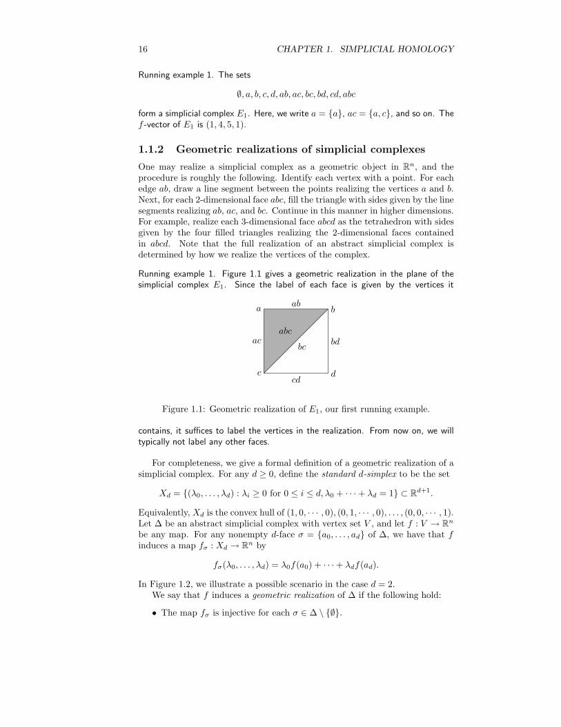
form a simplicial complex E1. Here, we write a = {a}, ac = {a, c}, and so on. Thef -vector of E1 is (1, 4, 5, 1).
1.1.2 Geometric realizations of simplicial complexes
One may realize a simplicial complex as a geometric object in Rn, and theprocedure is roughly the following. Identify each vertex with a point. For eachedge ab, draw a line segment between the points realizing the vertices a and b.Next, for each 2-dimensional face abc, fill the triangle with sides given by the linesegments realizing ab, ac, and bc. Continue in this manner in higher dimensions.For example, realize each 3-dimensional face abcd as the tetrahedron with sidesgiven by the four filled triangles realizing the 2-dimensional faces containedin abcd. Note that the full realization of an abstract simplicial complex isdetermined by how we realize the vertices of the complex.
Running example 1. Figure 1.1 gives a geometric realization in the plane of thesimplicial complex E1. Since the label of each face is given by the vertices it
a b
c d
ab
ac bd
cd
bc
abc
Figure 1.1: Geometric realization of E1, our first running example.
contains, it suffices to label the vertices in the realization. From now on, we willtypically not label any other faces.
For completeness, we give a formal definition of a geometric realization of asimplicial complex. For any d ≥ 0, define the standard d-simplex to be the set
Xd = {(λ0, . . . , λd) : λi ≥ 0 for 0 ≤ i ≤ d, λ0 + · · · + λd = 1} ⊂ Rd+1.
Equivalently, Xd is the convex hull of (1, 0, · · · , 0), (0, 1, · · · , 0), . . . , (0, 0, · · · , 1).Let ∆ be an abstract simplicial complex with vertex set V , and let f : V → Rn
be any map. For any nonempty d-face σ = {a0, . . . , ad} of ∆, we have that finduces a map fσ : Xd → Rn by
fσ(λ0, . . . , λd) = λ0f(a0) + · · · + λdf(ad).
In Figure 1.2, we illustrate a possible scenario in the case d = 2.We say that f induces a geometric realization of ∆ if the following hold:
• The map fσ is injective for each σ ∈ ∆ \ {∅}.

1.1. SIMPLICIAL COMPLEXES 17
(1, 0, 0)
(0, 1, 0)
(0, 0, 1)
f(a0)
f(a1)f(a2)
Figure 1.2: The map fσ transforms the standard 2-simplex on the left into thefilled triangle on the right, mapping (1, 0, 0) to f(a0), (0, 1, 0) to f(a1), and(0, 0, 1) to f(a2).
• For any nonempty σ, τ ∈ ∆, we have that
im fσ ∩ im fτ = im fσ∩τ ,
where im f denotes the image under f . Here, we adopt the conventionthat im f∅ = ∅.
The first condition is equivalent to saying that the point set {f(a) : a ∈ σ} isin general position. This means that there is no nontrivial linear combination∑
i λif(ai) = 0 such that∑
i λi = 0. The second condition is equivalent tosaying that
im fσ ∩ im fτ ⊆ im fσ∩τ ,
because we always have the other direction. In words, the intersection betweenthe realizations of any two faces contains nothing more than the realization ofthe greatest common face of the two simplices. The actual geometric realizationis the union
|∆| =⋃
σ∈∆\{∅}
im fσ.
Note that |∆| depends on the choice of vertex map f .
If ∆ has k vertices a1, . . . , ak, then we may realize ∆ in Rk by mapping ai toei, where ei denotes the ith unit vector in Rk. This is the standard geometricrealization of ∆, which is unique up to the order of the vertices.
Running example 2. Let E2 be the simplicial complex with vertices a+, a−, b+,b−, c+, and c− such that the maximal faces are all sets consisting of exactly oneelement from each of {a+, a−}, {b+, b−}, and {c+, c−}. Counting faces, oneobtains that E2 contains 6 vertices, 12 edges, and 8 triangles, which yields thef -vector (1, 6, 12, 8). On the left in Figure 1.3 is a geometric realization of E2 \{a−b−c−} in R2. On the right is a geometric realization of E2 in R3. Thisrealization is the boundary of an octahedron, one of the five Platonic solids.

18 CHAPTER 1. SIMPLICIAL HOMOLOGY
a−
b−
c−
a+
b+
c+ a−
b−
c−
a+
b+
c+
Figure 1.3: Geometric realizations of E2 \ {a−b−c−} (on the left) and E2 (onthe right), where E2 is our second running example.
Running example 3. Let E3 be the simplicial complex with vertex set {a, b, c, d, e, f}and with the following maximal faces:
abd, bce, acf, aef, bdf, cde, abe, bcf, acd, def.
Clearly, E3 is not a very big family; the f -vector is (1, 6, 15, 10). Nonetheless, thiscomplex is tricky to realize geometrically. In fact, it is impossible to realize it in R3
without some intersection of faces containing more than it should.2 Allowing somecheating, one may still illustrate E3 in R2 as a triangulated hexagon, as illustratedin Figure 1.4. Note that the boundary of this hexagon consists of two copies of eachof the vertices a, b, and c and also two copies of each of the edges ab, bc, and ac.To obtain a proper realization of E3, we need to identify all these pairs of copies.This cannot be done in R2 or even R3; we need a Euclidean space of dimension atleast four.
1.2 Oriented simplices
Let F be a commutative ring; the reader may think of F as the ring of integersZ or a field. Let ∆ be a simplicial complex. For each n ≥ −1, we form afree F-module Cn(∆; F) with a basis indexed by the n-dimensional faces of ∆.Specifically, for each face a0a1 · · · an, we have a basis element ea0,a1,...,an
. We
refer to a basis element as an oriented simplex. Note that the rank of Cn(∆; F)is the nth value fn(∆) in the f -vector of ∆. We refer to Cn(∆; F) is the chaingroup of degree n. This terminology stems from the fact that the modulesCn(∆; F) form a “chain” via certain maps to be discussed in Section 1.3. WhenF is clear from context, we will often write Cn(∆) = Cn(∆; F).
2The reason is that any geometric realization of E3 is homeomorphic to the real projectiveplane RP2, and there is no embedding of this topological space in R3.

1.2. ORIENTED SIMPLICES 19
a
bc
a
b c
d
e
f
Figure 1.4: Halfway to a geometric realization of E3, our third running example.To make this a true realization, we need to glue together opposite points on thehexagon.
Running examples. For E1 = {∅, a, b, c, d, ab, ac, bc, bd, cd, abc}, we get that
C−1(E1) = {λe∅ : λ ∈ F} ∼= F,
C0(E1) = {λaea + λbeb + λcec + λded : λa, λb, λc, λd ∈ F} ∼= F4,
C1(E1) = {λabea,b + · · · + λcdec,d : λab, . . . , λcd ∈ F} ∼= F5,
C2(E1) = {λea,b,c : λ ∈ F} ∼= F.
The chain groups for E2 and E3 are equally simple to describe.
The tilde symbol over C is a somewhat awkward convention among math-ematicians. Its only purpose is to indicate that we define the chain group ofdegree −1 to be F. Authors who adopt a strictly geometric viewpoint prefer todefine this group to be zero, because there is no sensible geometric interpretationof the empty set. Specifically, they define
Cn(∆; F) =
{Cn(∆; F) if n 6= −1,0 if n = −1.
For n ≥ 0, it turns out to be inconvenient to use the notation ea0,a1,...,anto
denote oriented simplices. Instead, we will write
a0 ∧ a1 ∧ · · · ∧ an = ea0,a1,...,an.
For example, a ∧ b represents the oriented simplex ea,b. In degree −1, we stickto the notation e∅.
The symbol ∧ denotes so-called exterior product. It satisfies the rules
b ∧ a = −a ∧ b
a ∧ a = 0
20 CHAPTER 1. SIMPLICIAL HOMOLOGY
for any oriented 0-simplices a and b. We may apply this rule to oriented simplicesin higher dimensions. For example,
b ∧ d ∧ a ∧ c = −b ∧ a ∧ d ∧ c = a ∧ b ∧ d ∧ c = −a ∧ b ∧ c ∧ d.
Here, each change of sign corresponds to interchanging two adjacent elements.Throughout Section 1.3, we will assume that this rule makes sense, is well-defined, and does not cause any contradictions. We postpone the formalities toSection 1.4.
1.3 Boundary maps
We define boundary maps ∂n, which are algebraic counterparts to the geometricnotion of oriented boundaries. The boundary map ∂n is a homomorphism thattakes an element x in Cn(∆) and associates to it an element in Cn−1(∆), theboundary of x.
Formally, we define ∂n on a given oriented simplex a0 ∧ a1 ∧ · · · ∧ an by
∂n(a0 ∧ a1 ∧ · · · ∧ an) =
n∑
r=0
(−1)ra0 ∧ · · · ∧ ar−1 ∧ ar ∧ ar+1 ∧ · · · ∧ an (1.1)
for each n, where ar denotes removal of the element ar. In the special casen = 0, we let ∂0(a) = e∅ for each vertex a. To obtain a homomorphism, weextend ∂n linearly to the whole of Cn(∆).
The boundary maps satisfy the equation ∂n ◦ ∂n+1 = 0; we always get zerowhen taking the boundary twice. Before proving this, we give some heuristicmotivation for why this is a desirable property of the boundary maps. Considerthe geometric notion of boundary in small dimensions. The boundary of a curveconsists of the two endpoints of the curve. If the curve is closed, then the twoendpoints coincide, which means that the curve does not have any boundary.Now, consider the unit circular disk. The boundary of this disk is a circle, whichis a closed curve. In particular, when taking the boundary of the boundary of thedisk, we are left with nothing. The same remains true for any “well-behaved”closed and bounded set in R2; the boundary of the boundary is empty, becausethe boundary is a closed curve, or the disjoint union of several closed curves.3
Interpreting a given edge ab as a line segment oriented from a to b, we define
∂1(a ∧ b) = b− a
and extend ∂1 linearly to the whole of C1(∆). The counterpart of a closed curvein our setting is the graph-theoretical concept of a set of edges forming a cycle,say a square {ab, bc, cd, da}. Now,
∂1(a ∧ b+ b ∧ c+ c ∧ d+ d ∧ a) = (b− a) + (c− b) + (d− c) + (a− d) = 0.
Thus the given definition indeed yields an algebraic counterpart of the fact thata closed curve has vanishing boundary.
3By the boundary of a d-dimensional manifold, we mean the set of points on the manifoldwith no open neighborhood homeomorphic to the open (d − 1)-ball.
1.3. BOUNDARY MAPS 21
a
b
c
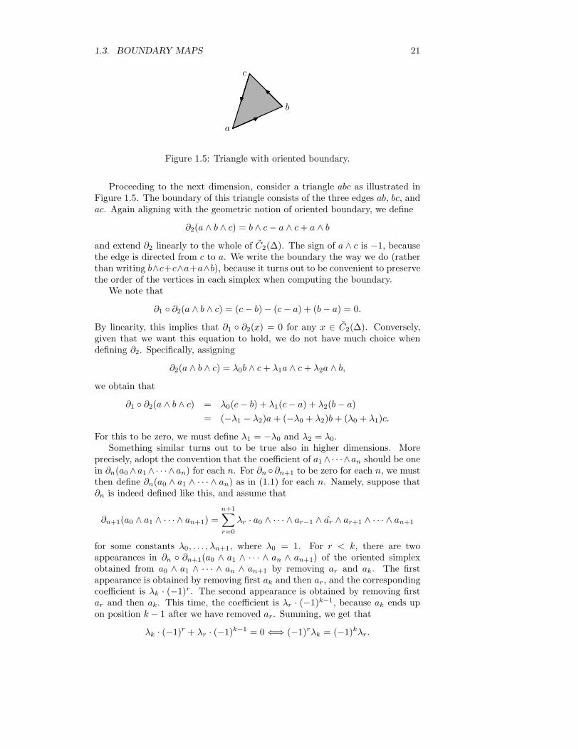
Figure 1.5: Triangle with oriented boundary.
Proceeding to the next dimension, consider a triangle abc as illustrated inFigure 1.5. The boundary of this triangle consists of the three edges ab, bc, andac. Again aligning with the geometric notion of oriented boundary, we define
∂2(a ∧ b ∧ c) = b ∧ c− a ∧ c+ a ∧ b
and extend ∂2 linearly to the whole of C2(∆). The sign of a ∧ c is −1, becausethe edge is directed from c to a. We write the boundary the way we do (ratherthan writing b∧c+c∧a+a∧b), because it turns out to be convenient to preservethe order of the vertices in each simplex when computing the boundary.
We note that
∂1 ◦ ∂2(a ∧ b ∧ c) = (c− b) − (c− a) + (b− a) = 0.
By linearity, this implies that ∂1 ◦ ∂2(x) = 0 for any x ∈ C2(∆). Conversely,given that we want this equation to hold, we do not have much choice whendefining ∂2. Specifically, assigning
∂2(a ∧ b ∧ c) = λ0b ∧ c+ λ1a ∧ c+ λ2a ∧ b,
we obtain that
∂1 ◦ ∂2(a ∧ b ∧ c) = λ0(c− b) + λ1(c− a) + λ2(b− a)
= (−λ1 − λ2)a+ (−λ0 + λ2)b + (λ0 + λ1)c.
For this to be zero, we must define λ1 = −λ0 and λ2 = λ0.Something similar turns out to be true also in higher dimensions. More
precisely, adopt the convention that the coefficient of a1∧· · ·∧an should be onein ∂n(a0 ∧a1∧ · · · ∧an) for each n. For ∂n ◦ ∂n+1 to be zero for each n, we mustthen define ∂n(a0 ∧ a1 ∧ · · · ∧ an) as in (1.1) for each n. Namely, suppose that∂n is indeed defined like this, and assume that
∂n+1(a0 ∧ a1 ∧ · · · ∧ an+1) =
n+1∑
r=0
λr · a0 ∧ · · · ∧ ar−1 ∧ ar ∧ ar+1 ∧ · · · ∧ an+1
for some constants λ0, . . . , λn+1, where λ0 = 1. For r < k, there are twoappearances in ∂n ◦ ∂n+1(a0 ∧ a1 ∧ · · · ∧ an ∧ an+1) of the oriented simplexobtained from a0 ∧ a1 ∧ · · · ∧ an ∧ an+1 by removing ar and ak. The firstappearance is obtained by removing first ak and then ar, and the correspondingcoefficient is λk · (−1)r. The second appearance is obtained by removing firstar and then ak. This time, the coefficient is λr · (−1)k−1, because ak ends upon position k − 1 after we have removed ar. Summing, we get that
λk · (−1)r + λr · (−1)k−1 = 0 ⇐⇒ (−1)rλk = (−1)kλr.

22 CHAPTER 1. SIMPLICIAL HOMOLOGY
Since λ0 = 1, this yields that λk = (−1)k for all k.By the above discussion, we obtain the desired double boundary condition:
Proposition 1.3.1 We have that ∂n ◦ ∂n+1 = 0 for every n.
An equivalent way of expressing Proposition 1.3.1 is to say that the sequence
C(∆) : · · ·∂n+2
−−−−→ Cn+1(∆)∂n+1
−−−−→ Cn(∆)∂n−−−−→ Cn−1(∆)
∂n−1
−−−−→ · · ·
defines a chain complex. We will discuss general chain complexes in Section 2.1.We refer to C(∆) as a simplicial chain complex.
Running example 1. The complex E1 has dimension 2, which means that we getthe following simplicial chain complex:
C(E1) : 0 −→ C2(E1)∂2−−−−→ C1(E1)
∂1−−−−→ C0(E1)∂0−−−−→ C−1(E1) −→ 0.
All other chain groups are zero. Remembering that E1 has f -vector (1, 4, 5, 1), weobtain that C(E1) has the following schematic structure:
0 −−−−→ F −−−−→ F5 −−−−→ F4 −−−−→ F −−−−→ 0.
1.4 Orientations of oriented simplices
We still have to settle the issue that there are different ways to arrange thevertices in an oriented simplex.
Start with the 1-dimensional case. There are two ways we may represent anedge ab as an oriented simplex: a ∧ b and b ∧ a. Yet, we want just one basiselement for each edge, not two. As already discussed in Section 1.2, we solvethis problem by making the identification
b ∧ a = −a ∧ b.
We think of a ∧ b and b ∧ a as having opposite orientations.Proceeding to dimension two, we may arrange the vertices a, b, and c of a face
abc in six different ways, which gives rise to six oriented simplices representingthe same face:
a ∧ b ∧ c a ∧ c ∧ b b ∧ a ∧ c b ∧ c ∧ a c ∧ a ∧ b c ∧ b ∧ a.
Again we want just one basis element, not six. We already gave an identificationrule in Section 1.2, which yields that
a ∧ b ∧ c = −b ∧ a ∧ c = b ∧ c ∧ a = −c ∧ b ∧ a = c ∧ a ∧ b = −a ∧ c ∧ b
In each step, we interchange two adjacent elements, and the sign changes ac-cordingly. One may check by hand that we obtain no contradictions.
Yet, we also need to check that the assignment of signs aligns with theboundary map. Again, this can be done by hand. For example,
∂2(b ∧ a ∧ c) = b ∧ a+ a ∧ c+ c ∧ b = −a ∧ b− b ∧ c+ a ∧ c = −∂2(a ∧ b ∧ c),
1.4. ORIENTATIONS OF ORIENTED SIMPLICES 23
which aligns with the assignment b ∧ a ∧ c = −a ∧ b ∧ c.To explain the general rule, fix a total order on the vertex set of ∆. For any
vertices x0, x1, . . . , xn forming an n-dimensional face, we define a pair (xi, xj)to be an inversion in x = x0 ∧ x1 ∧ · · · ∧ xn if i < j and xi > xj . For example,if a < b < c < d, then b ∧ d ∧ a ∧ c contains the three inversions (b, a), (d, a),and (d, c). We define inv(x) to be the number of inversions of x. For example,inv(b ∧ d ∧ a ∧ c) = 3.
Consider a face a0a1 · · ·an, assuming that a0 < a1 < · · · < an, and let πbe a permutation of {0, . . . , n}. Write br = aπ(r), a = a0 ∧ a1 ∧ · · · ∧ an, andb = b0 ∧ b1 ∧ · · · ∧ bn. We define
b = (−1)inv(b) · a. (1.2)
Lemma 1.4.1 The assignment (1.2) aligns with the boundary map ∂n. Equiva-lently, when computing ∂n(b) according to the rule (1.1), the result is (−1)inv(b) ·∂n(a).
Proof. Let ar be the oriented (n− 1)-dimensional simplex obtained from a byremoving ar, and define br analogously in terms of b and r. We obtain that
∂n(b) =
n∑
r=0
(−1)r · br =
n∑
r=0
(−1)r+inv(br) · aπ(r).
For the last step, we use the fact that br = aπ(r).It remains to prove that
inv(br) ≡ inv(b) + π(r) + r (mod 2). (1.3)
for each r. Namely, this will imply that
n∑
r=0
(−1)r+inv(br) · aπ(r) =
n∑
r=0
(−1)π(r)+inv(b) · aπ(r)
= (−1)inv(b) ·n∑
r=0
(−1)π(r) · aπ(r)
= (−1)inv(b) ·n∑
k=0
(−1)k · ak
= (−1)inv(b) · ∂n(a).
Now, let αr be the number of inversions of the form (bi, br) = (aπ(i), aπ(r))in b, and let βr be the number of inversions of the form (br, bi). Note that
inv(b) = inv(br) + αr + βr.
In particular, (1.3) yields that it suffices to prove that
αr + βr ≡ π(r) + r (mod 2). (1.4)
We have that αr is the number of elements among π(0), . . . , π(r − 1) that aregreater than π(r), whereas βr is the number of elements among π(r+1), . . . , π(n)

24 CHAPTER 1. SIMPLICIAL HOMOLOGY
that are less than π(r). Since there are r−αr elements among π(0), . . . , π(r−1)that are less than π(r), we conclude that βr = π(r)−(r−αr). As a consequence,
αr + βr = αr + π(r) − (r − αr) = 2αr + π(r) − r ≡ π(r) + r (mod 2),
which yields (1.4). �
In some situations, it might be convenient to extend the definition of a0 ∧a1∧· · ·∧an to the situation that ai = aj for some i and j. As indicated alreadyin Section 1.2, we then define a0 ∧ a1 ∧ · · · ∧ an to be zero. This is indeedcompatible with the boundary map. For example, if a0 = a1, then
∂n(a1 ∧ a1 ∧ · · · ∧ an) = a1 ∧ a2 ∧ · · · ∧ an − a1 ∧ a2 ∧ · · · ∧ an + w = w,
where w is a linear combination of elements all starting a1 ∧ a1, hence zero. Weleave the general case to the reader.
1.5 Products of chain group elements
It is possible to define some kind of product between chain group elements. Yet,for the product to be compatible with the boundary map (in a manner to bedescribed below), we must leave the product undefined for certain combinationsof elements. As a consequence, what we will consider is not a product in theproper sense of the word. In this context, it is worth mentioning the theoryof simplicial cohomology, a theory dual to the theory of simplicial homologyunder development in this document. Within that theory, it is indeed possibleto define a proper product.
For the purposes of this section, say that two oriented simplices a = a0 ∧· · · ∧ ar and b = b0 ∧ · · · ∧ bk are compatible if {a0, . . . , ar} ∪ {b0, . . . , bk} ∈ ∆.If a and b are compatible, we define the (exterior) product between a and b tobe
a ∧ b = a0 ∧ · · · ∧ ar ∧ b0 ∧ · · · ∧ bk.
By compatibility, this is either an oriented simplex in Cr+k−1(∆) or zero, thelatter being the case if ai = bj for some i and j.
More generally, suppose that c1 =∑
aλa · a ∈ Cr(∆) and
∑aµb · b ∈
Ck(∆) are two linear combinations of oriented simplices such that a and b arecompatible whenever λa 6= 0 and λb 6= 0. Then we may form the product
c1 ∧ c2 =∑
a,b
λaµb · a ∧ b ∈ Cr+k−1(∆).
We leave it to the reader to check that
c2 ∧ c1 = (−1)(r+1)(k+1)c1 ∧ c2
and
∂r+k−1(c1 ∧ c2) = ∂r(c1) ∧ c2 + (−1)r+1c1 ∧ ∂k(c2).
In particular, if c1 and c2 are both cycles, then c1 ∧ c2 is again a cycle.
1.6. DEFINITION OF SIMPLICIAL HOMOLOGY 25
Example. We have that
(a− b) ∧ (c− d) = a ∧ c− a ∧ d− b ∧ c+ b ∧ d,
(a− b) ∧ (a− c) = a ∧ a− a ∧ c− b ∧ a+ b ∧ c
= c ∧ a+ a ∧ b+ b ∧ c.
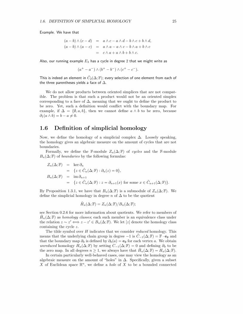
Also, our running example E3 has a cycle in degree 2 that we might write as
(a+ − a−) ∧ (b+ − b−) ∧ (c+ − c−).
This is indeed an element in C2(∆; F); every selection of one element from each ofthe three parentheses yields a face of ∆.
We do not allow products between oriented simplices that are not compat-ible. The problem is that such a product would not be an oriented simplexcorresponding to a face of ∆, meaning that we ought to define the product tobe zero. Yet, such a definition would conflict with the boundary map. Forexample, if ∆ = {∅, a, b}, then we cannot define a ∧ b to be zero, because∂1(a ∧ b) = b− a 6= 0.
1.6 Definition of simplicial homology
Now, we define the homology of a simplicial complex ∆. Loosely speaking,the homology gives an algebraic measure on the amount of cycles that are notboundaries.
Formally, we define the F-module Zn(∆; F) of cycles and the F-moduleBn(∆; F) of boundaries by the following formulas:
Zn(∆; F) = ker ∂n
= {z ∈ Cn(∆; F) : ∂n(z) = 0},
Bn(∆; F) = im ∂n+1
= {z ∈ Cn(∆; F) : z = ∂n+1(x) for some x ∈ Cn+1(∆; F)}.
By Proposition 1.3.1, we have that Bn(∆; F) is a submodule of Zn(∆; F). Wedefine the simplicial homology in degree n of ∆ to be the quotient
Hn(∆; F) = Zn(∆; F)/Bn(∆; F);
see Section 0.2.6 for more information about quotients. We refer to members ofHn(∆; F) as homology classes; each such member is an equivalence class underthe relation z ∼ z′ ⇐⇒ z− z′ ∈ Bn(∆; F). We let [z] denote the homology classcontaining the cycle z.
The tilde symbol over H indicates that we consider reduced homology. Thismeans that the underlying chain group in degree −1 is C−1(∆; F) = F · e∅ andthat the boundary map ∂0 is defined by ∂0(a) = e∅ for each vertex a. We obtainunreduced homology Hn(∆; F) by setting C−1(∆; F) = 0 and defining ∂0 to bethe zero map. In all degrees n ≥ 1, we always have that Hn(∆; F) = Hn(∆; F).
In certain particularly well-behaved cases, one may view the homology as analgebraic measure on the amount of “holes” in ∆. Specifically, given a subsetX of Euclidean space Rn, we define a hole of X to be a bounded connected
26 CHAPTER 1. SIMPLICIAL HOMOLOGY
component of Rn \X , the complement of X in Rn. For a given k ≥ 0, assumethat the (k+1)-skeleton ∆(k+1) of ∆ admits a geometric realization X in Rk+1.Then it is possible to prove that Hk(∆; F) is a free F-module of rank the numberof holes of X .
Running examples. The geometric realization of E1 in Figure 1.1 consists of onehole. Namely, the region in R2 surrounded by the three edges bc, cd, db is boundedand is separated by |E1| from the unbounded region outside |E1|. In Section 1.7.1,we show that H1(E1; F) indeed has rank one, and the homology class of the cycleb ∧ c+ c ∧ d+ d ∧ b is a generator of H1(E1; F).
The geometric realization X of E2 in Figure 1.3 also consists of one hole. Thisis because X divides R3 into one bounded region inside X and one unboundedregion outside X . Indeed, we will see that H2(E2; F) has rank one, and a generatoris given by the homology class of the cycle
(a+ − a−) ∧ (b+ − b−) ∧ (c+ − c−). (1.5)
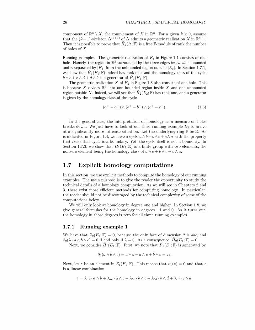
In the general case, the interpretation of homology as a measure on holesbreaks down. We just have to look at our third running example E3 to arriveat a significantly more intricate situation. Let the underlying ring F be Z. Asis indicated in Figure 1.4, we have a cycle a∧ b+ b∧ c+ c∧ a with the propertythat twice that cycle is a boundary. Yet, the cycle itself is not a boundary. InSection 1.7.3, we show that H1(E3; Z) is a finite group with two elements, thenonzero element being the homology class of a ∧ b+ b ∧ c+ c ∧ a.
1.7 Explicit homology computations
In this section, we use explicit methods to compute the homology of our runningexamples. The main purpose is to give the reader the opportunity to study thetechnical details of a homology computation. As we will see in Chapters 2 and3, there exist more efficient methods for computing homology. In particular,the reader should not be discouraged by the technical complexity of some of thecomputations below.
We will only look at homology in degree one and higher. In Section 1.8, wegive general formulas for the homology in degrees −1 and 0. As it turns out,the homology in those degrees is zero for all three running examples.
1.7.1 Running example 1
We have that Z2(E1; F) = 0, because the only face of dimension 2 is abc, and∂2(λ · a ∧ b ∧ c) = 0 if and only if λ = 0. As a consequence, H2(E1; F) = 0.
Next, we consider H1(E1; F). First, we note that B1(E1; F) is generated by
∂2(a ∧ b ∧ c) = a ∧ b− a ∧ c+ b ∧ c = z1.
Next, let z be an element in Z1(E1; F). This means that ∂1(z) = 0 and that zis a linear combination
z = λab · a ∧ b+ λac · a ∧ c+ λbc · b ∧ c+ λbd · b ∧ d+ λcd · c ∧ d,
1.7. EXPLICIT HOMOLOGY COMPUTATIONS 27
where λab, λac, λbc, λbd, λcd ∈ F. Note that
∂1(z) = ∂1(λab · a ∧ b+ λac · a ∧ c+ λbc · b ∧ c+ λbd · b ∧ d+ λcd · c ∧ d)
= (−λab − λac)a+ (λab − λbc − λbd)b
+ (λac + λbc − λcd)c+ (λbd + λcd)d.
Setting λab = t and λcd = u, this yields that λac = −t, λbd = −u, and λbc = t+u.In particular, Z1(E1; F) is generated by
z1 = a ∧ b− a ∧ c+ b ∧ c (t = 1, u = 0),
z2 = b ∧ c− b ∧ d+ c ∧ d (t = 0, u = 1).
To compute H1(E1; F), we note that x and y belong to the same homology classif and only if y − x is a multiple of z1, the generator of B1(E1; F). This meansthat the members of H1(E1; F) = Z1(E1; F)/B1(E1; F) are of the form
[uz2] = {tz1 + uz2 : t ∈ F}.
In particular, H1(E1; F) has dimension 1 and is generated by [z2].To summarize, we have the following result.
Proposition 1.7.1 We have that
Hn(E1; F) ∼=
{F if n = 1,0 if n 6= 1.
1.7.2 Running example 2
For convenience, we represent each face σ of E2 as a sequence rst, where r, s, t ∈{0, 1,×}. Specifically,
r =
0 if a+ ∈ σ,1 if a− ∈ σ,× if a+, a− /∈ σ.
The symbols s and t are defined analogously in terms of b± and c±, respectively.For example, 0×1 represents the face a+c−. We use the same sequences torepresent the corresponding oriented simplices.
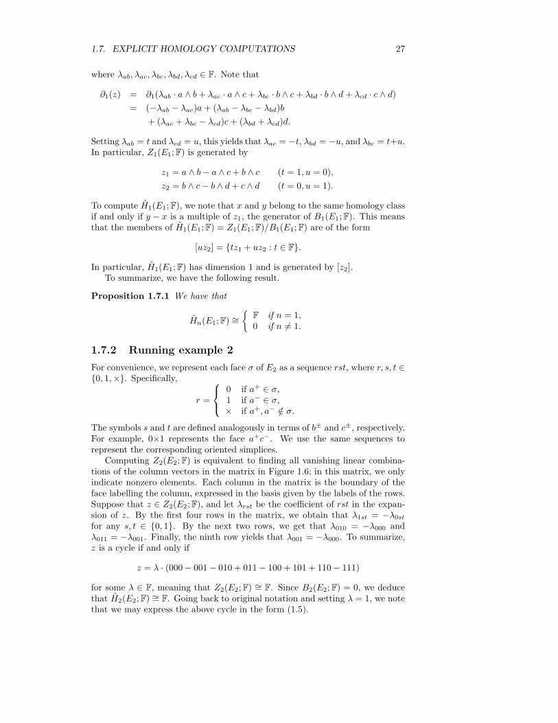
Computing Z2(E2; F) is equivalent to finding all vanishing linear combina-tions of the column vectors in the matrix in Figure 1.6; in this matrix, we onlyindicate nonzero elements. Each column in the matrix is the boundary of theface labelling the column, expressed in the basis given by the labels of the rows.Suppose that z ∈ Z2(E2; F), and let λrst be the coefficient of rst in the expan-sion of z. By the first four rows in the matrix, we obtain that λ1st = −λ0st
for any s, t ∈ {0, 1}. By the next two rows, we get that λ010 = −λ000 andλ011 = −λ001. Finally, the ninth row yields that λ001 = −λ000. To summarize,z is a cycle if and only if
z = λ · (000 − 001 − 010 + 011 − 100 + 101 + 110 − 111)
for some λ ∈ F, meaning that Z2(E2; F) ∼= F. Since B2(E2; F) = 0, we deducethat H2(E2; F) ∼= F. Going back to original notation and setting λ = 1, we notethat we may express the above cycle in the form (1.5).
28 CHAPTER 1. SIMPLICIAL HOMOLOGY
000 001 010 011 100 101 110 111
×00 1 1×01 1 1×10 1 1×11 1 10×0 −1 −10×1 −1 −11×0 −1 −11×1 −1 −100× 1 101× 1 110× 1 111× 1 1
.
Figure 1.6: Matrix describing the map ∂2 : C2(E2; F) → C1(E2; F).
×00 1×01 1×10 1×11 10×0 −1 −1 10×1 −1 −1 11×0 −11×1 −100× 1 1 −1 −1 101× 1 1 −110× 1 1 −111× 1
.
Figure 1.7: The result after applying a prudent choice of column operations onthe matrix in Figure 1.6.
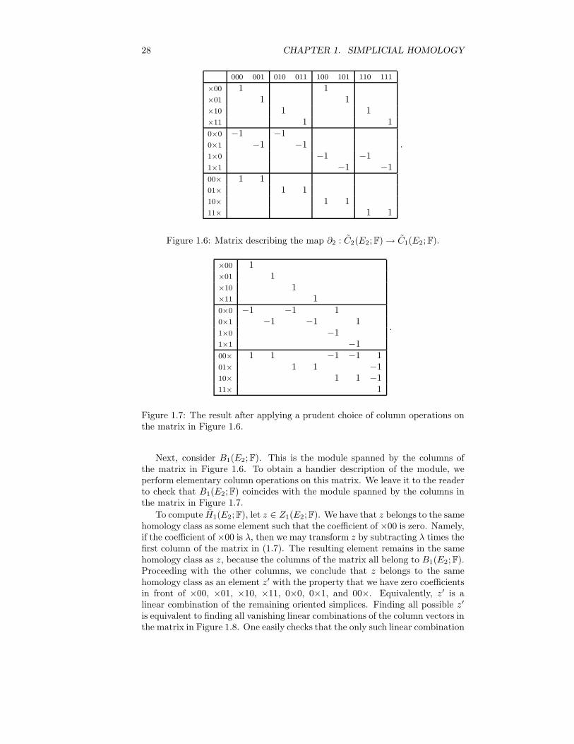
Next, consider B1(E2; F). This is the module spanned by the columns ofthe matrix in Figure 1.6. To obtain a handier description of the module, weperform elementary column operations on this matrix. We leave it to the readerto check that B1(E2; F) coincides with the module spanned by the columns inthe matrix in Figure 1.7.
To compute H1(E2; F), let z ∈ Z1(E2; F). We have that z belongs to the samehomology class as some element such that the coefficient of ×00 is zero. Namely,if the coefficient of ×00 is λ, then we may transform z by subtracting λ times thefirst column of the matrix in (1.7). The resulting element remains in the samehomology class as z, because the columns of the matrix all belong to B1(E2; F).Proceeding with the other columns, we conclude that z belongs to the samehomology class as an element z′ with the property that we have zero coefficientsin front of ×00, ×01, ×10, ×11, 0×0, 0×1, and 00×. Equivalently, z′ is alinear combination of the remaining oriented simplices. Finding all possible z′
is equivalent to finding all vanishing linear combinations of the column vectors inthe matrix in Figure 1.8. One easily checks that the only such linear combination

1.7. EXPLICIT HOMOLOGY COMPUTATIONS 29
1×0 1×1 01× 10× 11×
××0 1××1 1×0× 1×1× 1 10×× −11×× −1 −1 −1 −1
.
Figure 1.8: Matrix describing relevant parts of the map ∂1 : C1(E2; F) →C0(E2; F).
is the trivial one with all zeros. As a consequence, z′ = 0. The conclusion isthat there is just one single homology class, which is equivalent to saying thatH1(E2; F) is 0.
We summarize our results in a proposition.
Proposition 1.7.2 We have that
Hn(E2; F) ∼=
{F if n = 2,0 if n 6= 2.
1.7.3 Running example 3
Finally, we consider E3. The module Z2(E3; F) is given by all vanishing linearcombinations of the column vectors in the matrix in Figure 1.6.
abd bce caf aef bfd cde abe bcf cad defab 1 1bc 1 1ca 1 1ef 1 1fd 1 1de 1 1ad −1 1ae 1 −1af 1 −1be −1 1bf 1 −1bd 1 −1cf −1 1cd 1 −1ce 1 −1
.
Figure 1.9: Matrix describing the map ∂2 : C2(E3; F) → C1(E3; F).
Performing row operations, we arrive at the matrix in Figure 1.10. Notethat we have the element 2 in the lower right corner. This element could beeither nonzero or zero depending on the underlying ring F. Specifically, if F is Zor a field of characteristic different from 2, then the matrix has full rank, which

30 CHAPTER 1. SIMPLICIAL HOMOLOGY
means that H2(E3; F) = Z2(E3; F) = 0. If F is a field of characteristic two, thenthe last row of the matrix is zero. In this case, H2(E3; F) = Z2(E3; F) ∼= F, anda generator is given by the sum of all ten oriented simplices.
abd bce caf aef bfd cde abe bcf cad def1 1
1 11 1
1 11 1
1 11 1
1 11 1
2
.
Figure 1.10: The matrix in Figure 1.9 after a prudent choice of row operations.
Proceeding to degree 1, we obtain a nice description of B1(E3; F) by per-forming column operations on the matrix in Figure 1.9; see Figure 1.11 for theresulting matrix, whose columns span B1(E3; F). Note that the rightmost col-umn is equal to twice the cycle γ = −bf + bd + cf − cd = bd + dc + cf + fb.This column will be zero if F is a field of characteristic two.
ab 1bc 1ca 1ef 1fd 1de 1ad −1 1ae 1 −1 1af 1 −1 −1be −1 1 1bf 1 −1 −1 −2bd 1 −1 −1 1 2cf −1 1 2 2cd 1 −1 −2ce 1 −1 −1 −1
.
Figure 1.11: The matrix in Figure 1.9 after a prudent choice of column opera-tions.
To compute H1(E3; F), we proceed as with E2. Precisely, let z ∈ Z1(E2; F).We may use the first nine columns of the matrix in Figure 1.11 to get a cyclez′ in the same homology class as z such that the coefficients are zero in front ofab, bc, ca, de, ef, fd, ad, ae, be. It remains to determine all cycles that are linearcombinations of the remaining six basis elements af, bf, bd, cf, cd, ce. Two suchcycles belong to the same homology class if and only if they differ by a multipleof the cycle 2γ; this cycle is the rightmost column of the matrix in Figure 1.11.

1.8. HOMOLOGY IN LOW DEGREES 31
af bf bd cf cd cea −1b −1 −1c −1 −1 −1d 1 1e 1f 1 1 1
.
Figure 1.12: Matrix describing relevant parts of the map ∂1 : C1(E3; F) →C0(E3; F).
Looking at Figure 1.12, we draw the conclusion that all cycles are of theform λ · γ for some λ ∈ F. Two such cycles λ1γ and λ2γ belong to the samehomology class if and only if λ1 − λ2 = 2x for some x ∈ F.
To present a general formula for the homology of E3, we need the conceptof annihilator. For x ∈ F, we define AnnF(x) = {y ∈ F : xy = 0}.
Proposition 1.7.3 We have that
Hn(E3; F) ∼=
F/(2F) if n = 1,AnnF(2) if n = 2,0 if n /∈ {1, 2}.
For example,
Hn(E3; Q) ∼=
{Q/(2Q) = 0 if n = 1,AnnQ(2) = 0 if n = 2,
Hn(E3; Z) ∼=
{Z/(2Z) ∼= Z2 if n = 1,AnnZ(2) = 0 if n = 2,
Hn(E3; Z2) ∼=
{Z2/(2Z2) = Z2 if n = 1,AnnZ2
(2) = Z2 if n = 2.
1.8 Homology in low degrees
As promised, we give general formulas for the homology in degrees −1 and 0 ofa simplicial complex ∆. We also say a few words about the degree 1 in the casethat ∆ is a graph.
1.8.1 Homology in degree −1
Unless ∆ = ∅, we always have that Z−1(∆; F) = F · e∅. If ∆ = {∅}, thenB−1(∆; F) = 0, which means that H−1(∆; F) ∼= F. Otherwise, there is somevertex a in ∆. Since ∂0(a) = e∅, we get that B−1(∆; F) = Z−1(∆; F), whichmeans that H−1(∆; F) = 0. To summarize,
H−1(∆; F) ∼=
{F if ∆ = {∅},0 otherwise.
Note the distinction between the void simplicial complex ∅ containing nothingand the empty simplicial complex {∅} containing the empty set and nothingelse.
32 CHAPTER 1. SIMPLICIAL HOMOLOGY
1.8.2 Homology in degree 0
Let V be the vertex set of ∆. We note that a linear combination∑
a∈V λaabelongs to Z0(∆; F) if and only if
∑a∈V λa = 0. Namely, the boundary of λaa
is λae∅. The reader may check that Z0(∆; F) is a free F-module of rank |V |− 1.To determine B0(∆; F), define a relation ∼ on the vertex set of ∆ by letting
a ∼ b if and only if there is a edge path (a0a1, a1a2, . . . , am−1am) such thata = a0 and b = am. It is a simple exercise to show that ∼ defines an equivalencerelation. Let V1, V2, . . . , Vk be the equivalence classes, and fix a vertex ri in eachVi. For each a ∈ Vi \ {ri}, define a = a− ri. We claim that B0(∆; F) coincideswith the free submodule M of C0(∆; F) with basis X = {a : a ∈ Vi \ {ri}, 1 ≤i ≤ k}. In particular, B0(∆; F) has rank |V | − k.
To prove the claim, first note that B0(∆; F) is generated by all boundaries∂1(ab) = b− a such that ab is an edge of ∆. By definition, a ∼ b whenever ab isan edge in ∆, which implies that a and b belong to the same equivalence classVi. Since
∂1(ab) = b− a = (b− ri) − (a− ri) = b− a,
we conclude that B0(∆; F) is a submodule of M . For the reverse inclusion,it suffices to show that a is a boundary for each a ∈ Vi \ {ri} and for eachi such that 1 ≤ i ≤ k. Now a ∈ Vi if and only if there is an edge path(a0a1, a1a2, . . . , am−1am) such that ri = a0 and a = am. Observing that
∂1(a0a1 + a1a2 + · · · + am−1am) = am − a0 = a− ri = a,
we obtain the desired boundary.Now, the reader may check that we obtain a basis for Z0(∆; F) by adding
the element ri = ri − rk to the set X for 1 ≤ i ≤ k − 1. To conclude, H0(∆; F)is a free F-module of rank (|V | − 1)− (|V | − k) = k− 1, and a basis is given bythe homology classes of the elements r1, . . . , rk−1.
We refer to the equivalence classes V1, . . . , Vk as the connected componentsof ∆. By the above discussion, we may conclude the following.
Proposition 1.8.1 For any simplicial complex ∆, we have that
H0(∆; F) ∼= Fk−1,
where k is the number of connected components of ∆.
Using unreduced homology instead of reduced homology, we obtain the formulaH0(∆; F) ∼= Fk. This is one instance for which we get a nicer formula forunreduced homology than for reduced homology. As will be clear later on,there are other instances for which quite the opposite holds.
1.8.3 Homology in degree 1 for 1-dimensional complexes
As suggested by our treatment of our running example E3 in Section 1.7.3, thesituation in degree 1 is too complicated to allow for a simple formula like theone in Proposition 1.8.1. In the case that ∆ has no faces of dimension greaterthan one – i.e., ∆ is a graph – there is indeed a nice formula. Specifically, wethen have that
H1(∆; F) ∼= Fe−v+k,

1.8. HOMOLOGY IN LOW DEGREES 33
where e is the number of edges, v the number of vertices, and k the number ofconnected components of ∆. We leave the proof to the interested reader. Themodule H1(∆; F) is the cycle space of the graph ∆.

34 CHAPTER 1. SIMPLICIAL HOMOLOGY
Chapter 2
Combinatorial techniques
So far, our computations have been straightforward applications of linear alge-bra. Such a brute force approach works fine as long as the underlying simplicialcomplex is small enough, but once the complex grows too large, we need to findother means for computing the homology. In this chapter, we consider somemethods that are mainly combinatorial in nature. In Chapter 3, we proceedwith more algebraic methods.
2.1 General chain complexes
We will discuss methods that apply to a more general setting involving arbi-trary chain complexes, not just simplicial chain complexes. Moreover, we willfrequently need to transform simplicial chain complexes into new chain com-plexes that are not necessarily simplicial. For this reason, we introduce a moregeneral notion of chain complexes.
Let F be a commutative ring. A chain complex C over F is a sequence (Cn :n ∈ Z) of F-modules, called chain groups, along with F-module homomorphisms
dn : Cn → Cn−1
such that
dn ◦ dn+1 = 0 for n ∈ Z. (2.1)
We refer to dn as a boundary map. We always denote the boundary map bydn in the general case, thus reserving the notation ∂n for boundary maps insimplicial chain complexes.
As we did already in Section 1.3, one typically illustrates a chain complexas a sequence with arrows between the groups in the following manner:
C : · · ·dn+2
−−−−→ Cn+1dn+1
−−−−→ Cndn−−−−→ Cn−1
dn−1
−−−−→ · · ·
In this document, we will focus on finite chain complexes. In such complexes,only finitely many chain groups are nonzero. The simplicial chain complexassociated to a finite simplicial complex is always finite.
As in the case of simplicial complexes, we may define submodules of Cn
consisting of cycles and boundaries. More precisely, we define the F-module
35
36 CHAPTER 2. COMBINATORIAL TECHNIQUES
Zn(C) of cycles and the F-module Bn(C) of boundaries by the following formulas:
Zn(C) = ker ∂n = {z ∈ Cn : ∂n(z) = 0},
Bn(C) = im ∂n+1 = {z ∈ Cn : z = ∂n+1(x) for some x ∈ Cn+1}.
In any chain complex, we have that
Bn(C) ⊆ Zn(C).
Indeed, (2.1) is equivalent to saying that all boundaries are cycles. We definethe homology in degree n of C to be the quotient
Hn(C) =Zn(C)
Bn(C)=
ker dn
im dn+1.
What we refer to as the simplicial homology Hn(∆; F) of a simplicial complex∆ is really the homology Hn(C(∆; F)) of the simplicial chain complex C(∆; F)associated to ∆.
2.2 Splitting chain complexes
An important technique for computing the homology of a chain complex is tosplit it into smaller chain complexes. One may then compute the homology ofeach piece separately and finally add the pieces together to get the full homology.
To formalize this idea, we need a few concepts. Given a chain complex
C : · · ·dn+2
−−−−→ Cn+1dn+1
−−−−→ Cndn−−−−→ Cn−1
dn−1
−−−−→ · · ·
a subcomplex of C is a chain complex
C′ : · · ·dn+2
−−−−→ C′n+1
dn+1
−−−−→ C′n
dn−−−−→ C′n−1
dn−1
−−−−→ · · ·
such that the following hold:
• C′n is a submodule of Cn for each n.
• The restriction of dn to C′n defines a homomorphism to C′
n−1 for each n.Equivalently, dn(C′
n) ⊆ C′n−1 for each n.
The most important subcomplexes of a simplicial complex ∆ are the ones arisingfrom subcomplexes ∆0 of ∆.
Proposition 2.2.1 If ∆ is a simplicial complex and ∆0 is a subcomplex of ∆,then C(∆0) is a subcomplex of C(∆).
We leave the proof to the reader.A chain complex C splits into two chain complexes
C′ : · · ·dn+2
−−−−→ C′n+1
dn+1
−−−−→ C′n
dn−−−−→ C′n−1
dn−1
−−−−→ · · ·
C′′ : · · ·dn+2
−−−−→ C′′n+1
dn+1
−−−−→ C′′n
dn−−−−→ C′′n−1
dn−1
−−−−→ · · ·
if the following hold:
2.2. SPLITTING CHAIN COMPLEXES 37
• Each of C′ and C′′ is a subcomplex of C.
• Cn is the direct sum of C′n and C′′
n for each n.
We write C = C′ ⊕ C′′.
Theorem 2.2.2 If C = C′ ⊕ C′′, then
Hn(C) ∼= Hn(C′) ⊕Hn(C′′)
for every n.
Proof. We may write each element c ∈ Cn uniquely as a sum c′ + c′′, wherec′ ∈ C′
n and c′′ ∈ C′′n . To indicate that the sum is direct, we write c = c′ ⊕ c′′.
The boundary map has the property that
dn(c′ ⊕ c′′) = dn(c′) ⊕ dn(c′′).
In particular, dn(c′ ⊕ c′′) = 0 if and only if dn(c′) = dn(c′′) = 0, which meansthat
ker dn = (C′n ∩ ker dn) ⊕ (C′′
n ∩ ker dn).
For similar reasons, we have that
im dn = (C′n ∩ im dn) ⊕ (C′′
n ∩ im dn)
By Proposition 0.2.1, we get that
Hn(C) =(C′
n ∩ ker dn) ⊕ (C′′n ∩ ker dn)
(C′n ∩ im dn) ⊕ (C′′
n ∩ im dn)
∼=C′
n ∩ ker dn
C′n ∩ im dn
⊕C′′
n ∩ ker dn
C′′n ∩ im dn
.
= Hn(C′) ⊕Hn(C′′),
which concludes the proof. �
Running example 1. Let ∆0 be the subcomplex of E1 obtained by removing thefaces a, ab, ac, and abc. We claim that we may write C(E1) = C(E1; F) as thedirect sum of C(∆0) and the chain complex C′ with the following chain groups:
C′0 = 〈a− b〉,
C′1 = 〈ab, ac+ cb〉,
C′2 = 〈abc〉;
C′n = 0 for n /∈ {0, 1, 2}. Here, we use the notation (1) from Section 0.2.4, and we
write abc instead of a ∧ b ∧ c.To prove the claim, we first note that
∂(abc) = ab− (ac+ cb) ∈ C′1,
∂(ab) = ∂(ac+ cb) = b− a ∈ C′0,
∂(a− b) = 0 ∈ C′−1,
38 CHAPTER 2. COMBINATORIAL TECHNIQUES
which yields that C′ is a subcomplex of C(E1). By Proposition 2.2.1, C(∆0) is alsoa subcomplex. It remains to show that
Cn(E1) = C′n ⊕ Cn(∆0)
for each n. Now,
C′−1 ⊕ C−1(∆0) = 0 ⊕ 〈e∅〉,
C′0 ⊕ C0(∆0) = 〈a− b〉 ⊕ 〈b, c, d〉,
C′1 ⊕ C1(∆0) = 〈ab, ac+ cb〉 ⊕ 〈bc, bd, cd〉,
C′2 ⊕ C2(∆0) = 〈abc〉 ⊕ 0.
One easily checks that we indeed get Cn(E1) in each case, which concludes theproof of the claim. As a consequence,
Hn(E1) ∼= Hn(C′) ⊕ Hn(∆0).
We leave it to the reader to verify that C′ has zero homology and that Hn(∆0) iszero unless n = 1, in which case H1(∆0) ∼= F. Using Theorem 2.2.2, we hencereestablish the result from Section 1.7.1.
One may generalize Theorem 2.2.2 to the situation where C is the direct sumof k subcomplexes C(1), . . . ,C(k). By an induction argument, we get that
Hn(C) ∼= Hn(C(1)) ⊕ · · · ⊕Hn(C(k)). (2.2)
2.3 Collapses
Let σ and τ be faces of a simplicial complex ∆ such that the following hold:
• τ is maximal in ∆.
• σ = τ \ {x} for some x ∈ τ .
• τ is the only maximal face of ∆ containing σ.
The above conditions mean that the family ∆ \ {σ, τ} is a simplicial complex.We refer to the procedure of removing {σ, τ} from ∆ as an elementary collapse.
Proposition 2.3.1 For any elementary collapse ∆ → ∆\{σ, τ} = ∆0, we havethat
Hn(∆; F) ∼= Hn(∆0; F)
for all n.
Proof. Write k = dimσ = dim τ − 1. Let C′ be the subcomplex of C(∆) =C(∆; F) with the property that the nonzero chain groups are
C′k+1 = 〈τ〉,
C′k = 〈∂k+1(τ)〉.
This is indeed a chain complex, because ∂k+1(τ) ∈ C′k and ∂k(∂k+1(τ)) = 0 ∈
C′k−1. The reader may check that all homology groups of C′ are zero.

2.3. COLLAPSES 39
a b
c d
a b
c d
Figure 2.1: Elementary collapse with respect to the pair (ab, abc).
We claim that the chain complex C(∆) splits as
C(∆) = C′ ⊕ C(∆0).
By Theorem 2.2.2 and the fact that C′ has zero homology, this yields the propo-sition.
Now, it is clear that Ck+1(∆) is the direct sum of 〈τ〉 and Ck+1(∆0). More-over, we may write
Ck(∆) = 〈∂(τ)〉 + Ck(∆0), (2.3)
and this is again a direct sum. Namely, let x be an element in Ck(∆). Thecoefficient of σ in ∂(τ) is ±1. For simplicity, let us assume that the coefficientis 1. We may write x = λσ + x0 for some λ ∈ F and x0 ∈ Ck(∆0). Noting that
x = λσ + x0 = λ∂(τ) + λ(σ − ∂(τ)) + x0,
we obtain (2.3), because λ(σ − ∂(τ)) + x0 ∈ Ck(∆0). In addition, the sum isdirect. Namely, suppose that λ · ∂(τ) + x0 = 0. Then the coefficient of σ in x0
must be −λ, because the coefficient is +λ in ∂(τ). Yet, there is no occurrenceof σ in x0, which means that λ must be 0. As a consequence, x0 is also zero;hence the sum is direct. This concludes the proof. �
Running example 1. Look at the elementary collapse E1 → E1 \ {ab, abc} = E′1;
see Figure 2.1 for a geometric illustration. We obtain that
C−1(E1) = 0 ⊕ 〈e∅〉,C0(E1) = 0 ⊕ 〈a, b, c, d〉,C1(E1) = 〈ab− ac+ bc〉 ⊕ 〈ac, bc, bd, cd〉,
C2(E1) = 〈abc〉 ⊕ 0.
Proceeding with the elementary collapse E′1 → E′
1 \{a, ac} = ∆0, we may split thechain complex further as
C−1(E1) = 0 ⊕ 0 ⊕ 〈e∅〉,C0(E1) = 0 ⊕ 〈b− a〉 ⊕ 〈b, c, d〉,C1(E1) = 〈ab− ac+ bc〉 ⊕ 〈ac〉 ⊕ 〈bc, bd, cd〉,
C2(E1) = 〈abc〉 ⊕ 0 ⊕ 0.
The first two components of this direct sum form the subcomplex considered in theexample in Section 2.2.

40 CHAPTER 2. COMBINATORIAL TECHNIQUES
We refer to a sequence of elementary collapses
∆ = Σ0 → Σ1 → Σ2 → · · · → Σr = ∆0 (2.4)
as a collapse from ∆ to ∆0. Applying Proposition 2.3.1 r times, we obtain thefollowing important result.
Proposition 2.3.2 If there is a collapse from ∆ to ∆0, then
Hn(∆; F) ∼= Hn(∆0; F)
for every n.
In the example, we applied Proposition 2.3.1 twice to conclude that Hn(E1; F) ∼=Hn(∆0; F).
Let ∆0 be a simplicial complex, and let a be a vertex not in ∆0. The coneCone(∆0) = Conea(∆0) over ∆0 with apex a is the simplicial complex obtainedfrom ∆0 by adding σ ∪ {a} for each σ ∈ ∆0. Equivalently, ∆ is a cone withapex a if σ ∪ {a} is a face of ∆ whenever σ is a face of ∆.
Proposition 2.3.3 If ∆ is a cone with apex a, then Hn(∆; F) = 0 for every n.
Proof. We use induction on the number of faces of ∆. If ∆ is the void complex∅, then Cn(∆) = 0 and hence Hn(∆) = 0 for all n. Suppose that ∆ is nonempty,and let τ be a maximal face of ∆. We must have that τ is of the form σ ∪ {a}for some σ not containing a. Moreover, σ is not contained in any other faces,because if σ∪{x} is in ∆ for some x 6= a, then we also have that σ∪{x, a} ∈ ∆,contradicting the assumption that τ is maximal. We conclude that ∆ → ∆ \{σ, τ} = ∆′ defines an elementary collapse. Clearly, ∆′ is again a cone withapex a. By induction, Hn(∆′) = 0 for all n; hence Proposition 2.3.1 yields thatHn(∆) = 0 for all n. �
One may also prove Proposition 2.3.3 directly. Specifically, let z be a cycle inCn(∆; F). We may write z = c0+a∧c1, where c0, c1 are elements in Cn−1(∆0; F)and ∆ = Conea(∆0). We have that
0 = ∂n(z) = ∂n(c0) + c1 − a ∧ ∂n−1(c1).
For this to be zero, we need c1 = −∂(c0) and ∂n−1(c1) = 0. Yet, this meansthat
∂n+1(a ∧ c0) = c0 − a ∧ ∂n(c0) = c0 + a ∧ c1 = z;
hence z is a boundary. Since this is true for every cycle z, we conclude that thehomology is zero. The expression a ∧ c0 being a valid chain group element isbecause ∆ is a cone with apex a.
The full simplex on a vertex set V is the simplicial complex 2V of all subsetsof V . Writing d = |V | − 1, we refer to 2V as a d-simplex.
Corollary 2.3.4 If ∆ is a d-simplex for some d ≥ 0, then Hn(∆; F) = 0 forall n ≥ 0.

2.4. COLLAPSING IN PRACTICE 41
Proof. For any v in the vertex set of ∆, we have that ∆ is a cone with apex v.By Proposition 2.3.3, we are done. �
A complex ∆ is collapsible if there is a collapse from ∆ to the void complex∅ (not to be confused with {∅}). By the proof of Proposition 2.3.3, cones arecollapsible.
Corollary 2.3.5 If a complex ∆ is collapsible, then Hn(∆) = 0 for every n.
Proof. This is an immediate consequence of Proposition 2.3.2. �
There exist simplicial complexes ∆ that are not collapsible but still satisfyHn(∆; F) = 0 for all n.
2.4 Collapsing in practice
Suppose that we are given a simplicial complex ∆ and a subcomplex ∆0. Wewant to find out what it means for ∆ to admit a collapse to ∆0. By definition,there is then a sequence of elementary collapses as in (2.4). Let σi, τi be suchthat Σi−1 \Σi = {σi, τi} and σi ⊂ τi. Define M to be the set of pairs (σi, τi) for1 ≤ i ≤ r. This means that M is a matching of faces of ∆ such that every facenot in ∆0 appears in exactly one pair. Equivalently, M is a perfect matchingon ∆ \ ∆0.
Here, a matching on a family ∆ is a set M of pairs (σ, τ), where σ and τare distinct members of ∆, such that no member of ∆ appears in more thanone pair. The matching is perfect if every member appears in exactly one pair.Members of ∆ that appear in some pair are matched, whereas other membersare unmatched.
We say that a matching M on a family ∆ of sets is an element matching ifevery pair in M is of the form (σ \ {x}, σ ∪ {x}) for some x ∈ X and σ ∈ ∆.1
For simplicity, we will often write σ \ x = σ \ {x} and σ ∪ x = σ ∪ {x}. Allmatchings considered in this document are element matchings. By the abovediscussion, we conclude the following.
• For a simplicial complex ∆ to admit a collapse to a subcomplex ∆0, it isnecessary that there exists a perfect element matching on ∆ \ ∆0.
Yet, this condition is not sufficient. For example, ∆ = {∅, a, ab, b, bc, c, ac}cannot be collapsed to ∆0 = {∅}, but there is a perfect element matching on∆ \ ∆0 given by the pairs
(a, ab), (b, bc), (c, ac). (2.5)
The problem with this matching is that none of these pairs can be the pair usedin the first elementary collapse; each of a, b, and c belongs to two maximal faces,not just one.
As it turns out, there is a combinatorial description of the condition that aperfect element matching M on ∆\∆0 corresponds to a collapse. For generality,let ∆ be an arbitrary family of sets, and let M be an arbitrary element matchingon ∆. Form a directed graph D(∆,M) with one vertex for each member of ∆and with edges defined according to the following rules.
1Note that the pair is (σ, σ ∪ {x}) if x /∈ σ and (σ \ {x}, σ) if x ∈ σ.
42 CHAPTER 2. COMBINATORIAL TECHNIQUES
• There is a directed edge from σ \x to σ∪x whenever (σ \x, σ∪x) belongsto the matching M .
• There is a directed edge from σ ∪ x to σ \ x whenever (σ \ x, σ ∪ x) doesnot belong to the matching M .
We say that M is an acyclic matching if D(∆,M) does not contain any directedcycles.
Example. If M is the matching in (2.5), then D(∆,M) contains the directed cycle
a→ ab→ b→ bc→ c→ ac→ a.
In particular, M is not an acyclic matching.
ab
c d
e
f
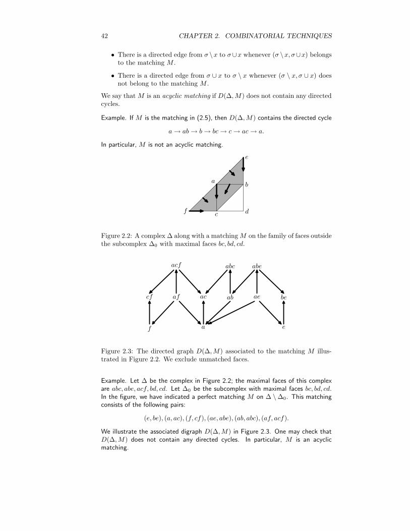
Figure 2.2: A complex ∆ along with a matchingM on the family of faces outsidethe subcomplex ∆0 with maximal faces bc, bd, cd.
f a e
cf af ac ab ae be
acf abc abe
Figure 2.3: The directed graph D(∆,M) associated to the matching M illus-trated in Figure 2.2. We exclude unmatched faces.
Example. Let ∆ be the complex in Figure 2.2; the maximal faces of this complexare abc, abe, acf, bd, cd. Let ∆0 be the subcomplex with maximal faces bc, bd, cd.In the figure, we have indicated a perfect matching M on ∆ \ ∆0. This matchingconsists of the following pairs:
(e, be), (a, ac), (f, cf), (ae, abe), (ab, abc), (af, acf).
We illustrate the associated digraph D(∆,M) in Figure 2.3. One may check thatD(∆,M) does not contain any directed cycles. In particular, M is an acyclicmatching.

2.4. COLLAPSING IN PRACTICE 43
τ0 τ1 τ2 τ3 · · · τr−2 τr−1
σ0 σ1 σ2 σ3 · · · σr−2 σr−1
Figure 2.4: Cycle in a digraph corresponding to a non-acyclic matching.
Proposition 2.4.1 Every directed cycle in D(∆,M) is of the form
(σ0, τ0, σ1, τ1, . . . , σr−1, τr−1)
such thatσi, σ(i+1) mod r ⊂ τi and (σi, τi) ∈M, (2.6)
and r ≥ 3; see Figure 2.4 for an illustration.
Proof. In a directed cycle in D(∆,M), the number of up-steps (steps of theform σ → σ ∪ x) is equal to the number of down-steps (steps of the formσ ∪ x → σ). There is no directed path (ρ, σ, τ) consisting of two consecutiveup-steps, as this would imply that σ is matched with both ρ and τ . As aconsequence, at most every other step can be an up-step. A straightforwardcounting argument yields that exactly every other step is an up-step. �
Proposition 2.4.2 There is a collapse from ∆ to ∆0 if and only if there existsa perfect acyclic matching M on ∆ \ ∆0.
Proof. Suppose that M is a perfect acyclic matching on ∆\∆0. Since D(∆,M)contains no directed cycles, there must be a face σ in ∆ \ ∆0 such that thereare no arrows directed to σ. Let τ be the face matched with σ. Since no arrowsare directed to σ, we must have that σ is the smaller face. Let a be such thatτ = σ∪a. Now, σ cannot be contained in any face τ ′ 6= τ of the same dimensionas τ , because then there would be an arrow from τ ′ to σ. Moreover, τ must bea maximal face of ∆, because if τ ∪ b belongs to ∆ for some b /∈ τ , then so does
(τ ∪ b) \ a = σ ∪ b,
which implies that there is an arrow from σ ∪ b to σ, a contradiction. As aconsequence,
∆ → ∆ \ {σ, τ}
is an elementary collapse. Proceeding inductively, we obtain a sequence ofelementary collapses from ∆ to ∆0.
The other direction is left to the reader. �
Example. With ∆, ∆0, and M defined as in Figure 2.2, we obtain a sequence ofelementary collapses by collapsing with the matched pairs in the following order:
(af, acf), (f, cf), (ae, abe), (e, be), (ab, abc), (a, ac).

44 CHAPTER 2. COMBINATORIAL TECHNIQUES
For example, we may start with (af, acf), because there is no arrow directed to afin D(∆,M); see Figure 2.3. As a consequence, ∆ can be collapsed to ∆0, whichmeans that Hn(∆) = Hn(∆0) for all n.
More generally, we have the following characterization of acyclic matchings.
Proposition 2.4.3 A matching M on a family ∆ is acyclic if and only if thematched pairs can be labelled (σ1, τ1), . . . , (σk, τk) such that the following condi-tions hold:
(i) For 1 ≤ i < j ≤ k, we have that dimσi ≤ dimσj .
(ii) For 1 ≤ i < j ≤ k, we have that σj is not contained in τi.
Proof. A matching M satisfying (i)-(ii) is acyclic. Namely, assume the op-posite, and let i be minimal such that τi appears in a cycle in D(∆,M). ByProposition 2.4.1, τi is followed in the cycle by σj and τj for some j 6= i (note thatthe indices i and j do not have the same meaning here as in that proposition).By (ii), we must have that j < i, which is a contradiction to the minimality ofi.
Conversely, suppose that M is acyclic. For any labeling (σ1, τ1), . . . , (σk, τk)of the matched pairs such that (i) is satisfied, we have that (ii) can only beviolated if dim σi = dimσj . In particular, we may restrict our attention to allmatched pairs (σ, τ) such that dimσ is equal to a fixed value. Since D(∆,M)does not contain any directed cycles, there must be some matched pair (σ1, τ1)with the property that τ1 does not contain σ for (σ, τ) ∈ M \ {(σ1, τ1)}. Byinduction on the size of M , the pairs in D(∆,M) \ {(σ1, τ1)} can be labelled as(σ2, τ2), . . . , (σk, τk) such that (ii) is satisfied. Adding (σ1, τ1} at the beginningof the list, we observe that (ii) is still satisfied. This concludes the proof. �
Example. Again, consider ∆, ∆0, and M defined as in Figure 2.2. The followingarrangement of the pairs in M satisfies the conditions in Proposition 2.4.3:
(a, ac), (e, be), (f, cf), (ab, abc), (ae, abe), (af, acf).
We obtain a collapse from ∆ to ∆0 by starting with the pair on the far right andthen going left. There are many other possible arrangements, but the pair (ab, abc)must appear before the pair (ae, abe), because abe contains ab.
We conclude the section with some useful results. See Section 2.7 for exam-ples.
A finite partially ordered set or poset is a pair P = (X,≤), where X is afinite set and ≤ is a binary relation on X satisfying the following conditions forall x, y, z ∈ X :
• x ≤ x.
• If x ≤ y and y ≤ x, then x = y.
• If x ≤ y and y ≤ z, then x ≤ z.

2.4. COLLAPSING IN PRACTICE 45
An (order-preserving) poset map between two posets P = (X,≤P ) and Q =(Y,≤Q) is a function f : X → Y such that f(x) ≤Q f(y) whenever x ≤P y. Wewill often write f : P → Q. We obtain a poset structure on a family ∆ of setsby definining σ ≤ τ whenever σ ⊆ τ .
Lemma 2.4.4 ([1, 2]) (Cluster Lemma) Let ∆ be a family of sets, and letf : ∆ → Q be a poset map, where Q is an arbitrary poset. For q ∈ Q, let Mq bean acyclic matching on
f−1(q) = {σ ∈ ∆ : f(σ) = q}.
Let
M =⋃
q∈Q
Mq.
Then M is an acyclic matching on ∆.
Proof. Assume the opposite, and let (σ0, τ0, . . . , σr−1, τr−1) be a cycle inD(∆,M) satisfying (2.6). Let q0, . . . , qr−1 be such that σk, τk ∈ f−1(qk) for 0 ≤k ≤ r − 1. Since σ(k+1) mod r ⊂ τk, we get that q(k+1) mod r = f(σ(k+1) mod r) ≤f(σk) = qk. Via a simple induction argument, this implies that qk′ ≤ qk for anypair k, k′. Swapping k and k′, we obtain qk ≤ qk′ , which implies that qk = qk′ ; Qis a poset. Hence all sets in the cycle are contained in one single family f−1(q),which is a contradiction. �
A very common situation is described in the following corollary.
Corollary 2.4.5 Let ∆ be a family of subsets of a set X, and let Y be a subsetof X. For ρ ⊆ Y , let Mρ be an acyclic matching on the family
∆ρ = {σ ∈ ∆ : σ ∩ Y = ρ}.
Define
M =⋃
ρ⊆Y
Mρ.
Then M is an acyclic matching on ∆.
Proof. Let 2Y denote the poset of all subsets of Y ordered by inclusion. Aposet map from ∆ to 2Y is given by mapping a face σ to σ ∩ Y . Namely, ifσ ⊆ τ , then σ ∩ Y ⊆ τ ∪ Y . By Lemma 2.4.4, we are done. �
Our final lemma gives another approach to constructing acyclic matchings.The idea is to pick an element x and match σ \ x with σ ∪ x whenever possible.
Lemma 2.4.6 Let ∆ be a family of subsets of a set X, and let x ∈ X. Define
Mx = {(σ \ x, σ ∪ x) : σ \ x, σ ∪ x ∈ ∆};
∆x = {σ : σ \ x, σ ∪ x ∈ ∆}.
Let M ′ be an acyclic matching on ∆′ = ∆ \ ∆x. Then M = Mx ∪M ′ is anacyclic matching on ∆.
46 CHAPTER 2. COMBINATORIAL TECHNIQUES
Proof. Assume that (σ0, τ0, . . . , σr−1, τr−1) is a cycle in D(∆,M) satisfying(2.6). Since M ′ is an acyclic matching on ∆′, there must be some pair {σi, τi}that is included in Mx rather than in M ′; by construction, we then have thatτi = σi∪x. For simplicity, assume that i = 0. Since τr−1 is not matched with σ0,we must have that x /∈ τr−1. This means that there is some j ∈ {1, . . . , r − 1}such that x ∈ τj−1 and x /∈ τj . However, this implies that τj−1 = σj ∪ x,which is a contradiction, because we would then have that (σj , τj−1) ∈ Mx byconstruction. �
2.5 Basics of discrete Morse theory
Now, we generalize the situation from Section 2.3. The topics discussed in thissection form the basis of discrete Morse theory, a method introduced by RobinForman.
Let
C : · · ·dn+2
−−−−→ Cn+1dn+1
−−−−→ Cndn−−−−→ Cn−1
dn−1
−−−−→ · · ·
be an arbitary chain complex C of free and finitely generated F-modules. Weassume that we have a fixed basis En of each Cn. For example, if C is thesimplicial chain complex associated to a simplicial complex, then we may chooseEn to be the usual set of oriented simplices of dimension n. For simplicity, wewrite d = dn for each n.
Any element c in Cn admits a unique representation
c =∑
σ∈En
λσσ
as a linear combination of the basis elements, where λσ ∈ F for each σ. Werefer to λσ as the coefficient of σ in c. For x ∈ Cn+1, we let (x : σ) denote thecoefficient of σi in d(x).
Let k be an integer, and let σ ∈ Ek and τ ∈ Ek+1. We want to define theconcept of a generalized elementary collapse involving the pair (σ, τ). It turnsout to be convenient to drop the maximality requirements on τ . In the simplicialcase, this leaves us with one single requirement:
• σ = τ \ x for some x ∈ τ .
In the general case, we require the following:
• The coefficient (τ : σ) of σ in d(τ) is invertible in F.
In the case that F is a field, this means that the given coefficient is a nonzeroelement in F. If F = Z, then the coefficient must be 1 or −1.
Given an elementary collapse from a simplicial complex ∆ to a subcomplex∆0, we deduced in Section 2.3 that C(∆) can be written as a direct sum C′ ⊕C(∆0), where C′ has zero homology. In our more general setting, we want to
obtain a similar decomposition C = C′ ⊕ C, where again C′ has zero homology.As we will see, the procedure is a little bit more complicated than in Section 2.3.
To start with, let
Ek+1 = Ek+1 \ {τ}
Ek = Ek \ {σ}.
2.5. BASICS OF DISCRETE MORSE THEORY 47
Defining En = En for all other choices of n, we obtain a new family of F-modulesCn, where Cn is the free F-module with basis En. Yet, we get two problems; forsimplicity we write d = dn for all n.
1. It is not necessarily true that d(x) ∈ Ck for all x ∈ Ck+1, because wemight have that (x : σ) 6= 0.
2. It is not necessarily true that d(x) ∈ Ck+1 for all x ∈ Ck+2, because wemight have that (x : τ) 6= 0.
These problems are a consequence of our dropping the maximality requirementson τ . We start by taking care of the first problem. As it turns out, our solutionto this problem will also solve the second problem.
For any basis element ǫ ∈ Ek+1 \ {τ}, define
λǫ =(ǫ : σ)
(τ : σ)
and
ǫ = ǫ− λǫτ = ǫ−(ǫ : σ)
(τ : σ)· τ.
Note that
(ǫ : σ) = (ǫ : σ) − λǫ(τ : σ) = (ǫ : σ) −(ǫ : σ)
(τ : σ)· (τ : σ) = 0.
In particular, d(ǫ) ∈ Ck. Redefine Ek+1 as
Ek+1 = {ǫ : ǫ ∈ Ek+1 \ {τ}}.
Moreover, redefine Ck+1 to be the free F-module with basis Ek+1.
Example. Consider the chain complex corresponding to the simplicial complex con-sisting of all subsets of the set {r, s, t, u}. Consider the pair (σ, τ), where σ = rtand τ = rst. In this case, k = 1. Note that
(rst : rt) = −1,
because the coefficient of rt in ∂(rst) = rs + st− rt is −1.Now, look at the basis elements ǫ 6= rst in degree 2. We have that
λǫ =(ǫ : rt)
(rst : rt)= −(ǫ : rt),
which yields thatλrsu = −(rsu : rt) = 0,λrtu = −(rtu : rt) = −1,λstu = −(stu : rt) = 0.
This means that we should define
rsu = rsu − 0 = rsu,
rtu = rtu − (−rst) = rtu + rst,
stu = stu− 0 = stu.

48 CHAPTER 2. COMBINATORIAL TECHNIQUES
One easily checks that rt does not appear in the boundary of any of these elements.For example,
∂(rtu) = ∂(rtu + rst) = rt+ tu− ru + rs+ st− rt
= rs− ru + st+ tu.
After having solved the first problem, it remains to consider the secondproblem: We want d(x) to lie in Ck+1 for every x ∈ Ck+2 = Ck+2. Now,
Ek+1 ∪ {τ} is a basis for Ck+1. In particular, there are numbers µǫ such that
d(x) =∑
ǫ∈Ek+1\{τ}
µǫǫ+ µττ.
Since d2(x) = 0, we get that
0 = (d(x) : σ) =∑
ǫ∈Ek+1\{τ}
µǫ(ǫ : σ) + µτ (τ : σ) = µτ (τ : σ).
The last equality is a consequence of the fact that (ǫ : σ) = 0 for all ǫ ∈ Ek+1\{τ}.Since (τ : σ) is invertible, we obtain that µτ must be zero. As a consequence,
d(x) ∈ Ck+1.
Example. Let us continue with the same example as before. Since k = 1, we wantto check that d(x) ∈ C2 for each x ∈ C3. Now, C3 = 〈rstu〉, and we get that
∂(rstu) = stu− rtu + rsu− rst = stu− (rtu + rst) + rsu = stu− rtu + rsu.
This indeed belongs to C2.
We may conclude the following.
Proposition 2.5.1 Let σ ∈ Ek and τ ∈ Ek+1 be such that (τ : σ) is invertiblein F. Then
C : · · ·dn+2
−−−−→ Cn+1dn+1
−−−−→ Cndn−−−−→ Cn−1
dn−1
−−−−→ · · ·
defines a chain complex, where Cn is the submodule of Cn with basis
En =
{ǫ− (ǫ:σ)(τ :σ) · τ : ǫ ∈ Ek+1} if n = k + 1,
Ek \ {σ} if n = k,En otherwise.
Let C′ be the subcomplex of C with the property that the nonzero chain groupsare C′
k+1 = 〈τ〉 and C′k = 〈d(τ)〉. We obtain the following.
Proposition 2.5.2 Let C be defined as in Proposition 2.5.1. Then C is thedirect sum of C′ and C. In particular, Hn(C) ∼= Hn(C) for each n.

2.6. JOINS, DELETIONS, AND LINKS 49
Proof. We already concluded that C is a subcomplex of C. As a consequence,it suffices to show that Cn is the direct sum of C′
n and Cn for each n. Thisis immediate unless n ∈ {k, k + 1}. For n = k, the proof is identical to thatof Proposition 2.3.1. For n = k + 1, it is easy to check that we obtain a basisfor Ck+1 by adding τ to Ek+1. To prove the final statement in the proposition,apply Theorem 2.2.2 and use the fact that the homology of C′ is zero. �
After having considered the situation for one single matched pair, we nowconsider a general matching
M = {(σi, τi) : 1 ≤ i ≤ r},
where σi and τi are basis elements such that 〈∂(τi), σi〉 is invertible for each i.For any x ∈ Cd, we write deg x = d.
Theorem 2.5.3 Suppose that the following hold:
(i) For 1 ≤ i < j ≤ r, we have that dimσi ≤ dimσj.
(ii) For 1 ≤ i < j ≤ r, we have that 〈∂(τi), σj〉 is zero.
Then it is possible to form a new chain complex C such that Hn(C) ∼= Hn(C) for
all n and such that the rank of Cn is equal to the rank of Cn minus the numberof basis elements e ∈ {σi, τi, : 1 ≤ i ≤ r} such that deg e = d.
For simplicial chain complexes, conditions (i)-(ii) are equivalent to saying thatthe matching is acyclic; apply Proposition 2.4.3.
Let us sketch a proof. Starting with the very last pair (σk, τk), we may
use the above procedure to transform C into a new chain complex C with thesame homology as C. If k = 1, then we are done. Otherwise, we observe thefolloing: When moving from C to C, we only modify basis elements e suchthat 〈∂(e), σk〉 6= 0. Among the elements σ1, τ1, . . . , σk−1, τk−1, there is no suchelement by assumption. In particular, conditions (i)-(ii) still hold for the pairs
(σ1, τ1), . . . , (σk−1, τk−1) in C. Using an induction argument, we may hence
transform C into a chain complex with properties as in the theorem.
2.6 Joins, deletions, and links
Some important constructions in the theory of simplicial complexes are those ofjoins, deletions, and links.
2.6.1 Joins
Let X and Y be two sets such that X∩Y is empty. Let ∆ be a family of subsetsof X , and let Γ be a family of subsets of Y . The join of ∆ and Γ is the family
∆ ∗ Γ = {δ ∪ γ : δ ∈ ∆, γ ∈ Γ}.
Observe that ∆ ∗ ∅ = ∅ and ∆ ∗ {∅} = ∆. If both ∆ and Γ are simplicialcomplexes, then ∆ ∗ Γ is also a simplicial complex.
For example, any cone is a join, because
Conea(Γ) = {∅, a} ∗ Γ.
50 CHAPTER 2. COMBINATORIAL TECHNIQUES
See Section 2.3 for more discussion on cones.For another important special case, let Γ be a simplicial complex, and let a
and b be two vertices not in Γ. The suspension Susp(Γ) = Suspa,b(Γ) is the join{∅, a, b} ∗ Γ. Equivalently,
Susp(Γ) = {σ, σ ∪ {a}, σ ∪ {b} : σ ∈ Γ}.
We examine suspensions in Section 2.6.2.Given a matching M∆ on ∆ and a subfamily Γ0 of Γ, we define
M∆ ∗ Γ0 = {(σ ∪ γ, τ ∪ γ) : (σ, τ) ∈M∆, γ ∈ Γ0}. (2.7)
If M∆ is a perfect matching on ∆, then M∆ ∗Γ0 is a perfect matching on ∆∗Γ0.We define ∆0 ∗MΓ analogously for any subfamily ∆0 of ∆ and any matchingMΓ on Γ.
In the following, δ always denotes a member of ∆, whereas γ denotes amember of Γ.
Proposition 2.6.1 Let X and Y be two sets such that X ∩ Y is empty. Let ∆be a family of subsets of X, and let Γ be a family of subsets of Y . Suppose thatwe have acyclic matchings M∆ and MΓ on ∆ and Γ, respectively. Then thereis an acyclic matching on ∆ ∗Γ such that δ ∪ γ is unmatched if and only if δ isunmatched with respect to M∆ and γ is unmatched with respect to MΓ.
Proof. Define a matching M on ∆ ∗ Γ as the union of the following twomatchings.
• M∆ ∗ Γ.
• C ∗MΓ, where C is the family of members of ∆ that are unmatched withrespect to M∆.
Note the asymmetry in the construction. It is clear that δ ∪ γ is unmatched ifand only if δ is unmatched with respect to M∆ and γ is unmatched with respectto MΓ.
It remains to prove that M is an acyclic matching. Assume the opposite,and let
(δ0 ∪ γ0, δ1 ∪ γ1, . . . , δ2r−1 ∪ γ2r−1)
be a cycle in D(∆ ∗ Γ,M). Consider the sequence
(δ0, δ1, . . . , δ2r−1).
By construction, for each i, we have that either δi = δi+1 or there is a directededge from δi to δi+1 in D(∆,M∆) (indices are computed modulo 2r). SinceD(∆,M∆) is acyclic, we must have that δi = δi+1 for all i, which yields that allδi are equal to some fixed δ.
If δ is matched in M∆, then there cannot be a directed edge from δ ∪ γ toδ∪γ′ unless γ′ ⊂ γ. This rules out the existence of a directed cycle in this case.
Suppose that δ is unmatched in M∆, and consider the sequence
(γ0, γ1, . . . , γ2r−1).
Again by construction, this sequence forms a directed cycle in D(Γ,MΓ), acontradiction. �
2.6. JOINS, DELETIONS, AND LINKS 51
Corollary 2.6.2 Suppose that ∆ admits a collapse to ∆0 and that Γ admits acollapse to Γ0. Then ∆ ∗ Γ admits a collapse to ∆0 ∗ Γ0.
Proof. The given conditions are equivalent to ∆ \ ∆0 and Γ \ Γ0 admittingacyclic matchings. Proposition 2.6.1 yields that ∆ ∗ Γ \ (∆0 ∗ Γ0) admits aperfect acyclic matching. By Proposition 2.4.2, this is equivalent to saying that∆ ∗ Γ admits a collapse to ∆0 ∗ Γ0. �
In particular, the following is true.
Corollary 2.6.3 Let ∆ and Γ be simplicial complexes. If ∆ is collapsible, then∆ ∗ Γ is collapsible.
2.6.2 Links and deletions
Let ∆ be a simplicial complex, and let a be a vertex in ∆. The deletion of ∆with respect to a is the subcomplex
del∆(a) = {σ ∈ ∆ : a /∈ σ}.
The link of ∆ with respect to a is the subcomplex
link∆(a) = {σ ∈ del∆(a) : σ ∪ {a} ∈ ∆}.
Note that ∆ is the disjoint union of del∆(a) and {a} ∗ link∆(a).The following proposition is a special case of a more general result discussed
in Section 3.3. Since we will need the proposition already in Section 2.7, we givea separate proof here.
Proposition 2.6.4 Let n be integer, let ∆ be a simplicial complex, and let a bea vertex such that Hn(del∆(a); F) = Hn−1(del∆(a); F) = 0. Then
Hn(∆; F) ∼= Hn−1(link∆(a); F).
Proof. Write D = del∆(a) and L = link∆(a). We may write any element z inCn(∆) as a sum z = x+ a ∧ y, where x ∈ Cn(D) and y ∈ Cn−1(L). Note thatz is a cycle if and only if ∂n(x) + y = 0 and ∂n−1(y) = 0. In particular, we maywrite any element z in Zn(∆) as a sum z = x − a ∧ ∂n(x), where x ∈ Cn(D)and ∂n(x) ∈ Cn−1(L). Also note that we may write any element z in Bn(∆) as
z = ∂n+1(x+ a ∧ y) = ∂n+1(x) + y − a ∧ ∂n(y)
for some x ∈ Cn+1(D) and y ∈ Cn(L).Define a map ϕ : Cn(∆) → Cn−1(L) by
ϕ(x + a ∧ y) = y.
By the above discussion, ϕ induces a map ϕ∗ : Hn(∆) → Hn−1(L). Namely,if z ∈ Zn(∆), then ϕ(z) is of the form −∂n(x) for some x ∈ Cn(D) such that∂n(x) ∈ Cn−1(L), hence an element in Zn−1(L). If z ∈ Bn(∆), then ϕ(z) is ofthe form ∂n(y) for some y ∈ Cn(L), hence an element in Bn−1(L).
It remains to prove that ϕ∗ is an isomorphism. First, assume that z is anelement in Zn(∆) such that ϕ(z) is an element in Bn−1(L). Writing z = x−a∧
52 CHAPTER 2. COMBINATORIAL TECHNIQUES
∂n(x), where x ∈ Cn(D) and ∂n(x) ∈ Cn−1(L), we obtain that ϕ(z) = −∂n(x).This belonging to Bn−1(L) means that ∂n(x) = ∂n(x′) for some x′ ∈ Cn(L).Now,
z − ∂n+1(a ∧ x′) = x− a ∧ ∂n(x) − x′ + a ∧ ∂n(x′)
= x− x′ ∈ Zn(D) = Bn(D);
the last equality follows from the fact that Hn(D) = 0. As a consequence,z ∈ Bn(∆), which yields that ϕ∗ is injective.
Next, let w be any element in Zn−1(L). Since Zn−1(D) = Bn−1(D), we havethat w = ∂n(x) for some x ∈ Cn(D). This yields that z = −x+ a ∧ ∂n(x) is anelement in Zn(∆) such that ϕ(z) = w. In particular, ϕ∗ is surjective. �
Corollary 2.6.5 We have that Hn(Suspa,b(Γ); F) = Hn−1(Γ; F) for every n.
Proof. Write ∆ = Suspa,b(Γ). We observe that
del∆(a) = Coneb(Γ),
link∆(a) = Γ.
Using Proposition 2.3.3, we deduce that Hn(del∆(a); F) = 0 for all n. As aconsequence, Proposition 2.6.4 yields that
Hn(∆; F) ∼= Hn−1(link∆(a); F) = Hn−1(Γ; F),
which concludes the proof. �
Running example 2. We have that E2 is a triple suspension of {∅}. Specifically,define Σ0 = {∅},
Σ1 = Suspa+,a−(Σ0) = {∅, a+, a−},Σ2 = Suspb+,b−(Σ1) = {∅, a+, a−, b+, b−, a+b+, a+b−, a−b+, a−b−},Σ3 = Suspc+,c−(Σ2).
Then E2 = Σ3. Since Hn(Σ0; F) ∼= F if n = −1 and Hn(Σ0; F) ∼= 0 otherwise,Corollary 2.6.5 applied three times yields that Hn(E2; F) ∼= F if n = −1 + 3 = 2and Hn(E2; F) ∼= 0 otherwise. Hence we reestablish the result from Section 1.7.2.
Corollary 2.6.5 is also a special case of a general result about joins, whichwe state for completeness.
Theorem 2.6.6 Let ∆ be a simplicial complex such that all homology groupsof ∆ are free F-modules. Let Γ be any simplicial complex. Then
Hn(∆ ∗ Γ; F) ∼=⊕
i+j=n−1
Hi(∆; F) ⊗F Hj(Γ; F).
Here, A⊗FB is the tensor product over F of the two F-modules A and B. In thecase that A and B are free F-modules with bases {e1, . . . , er} and {e′1, . . . , e
′s},
respectively, the tensor product A ⊗F B is the free F-module of rank rs withbasis {ei ⊗ e′j : 1 ≤ i ≤ r, 1 ≤ j ≤ s}. We refer the interested reader to atextbook in algebra for the general definition and to a textbook in algebraictopology for a proof of Theorem 2.6.6.
2.7. INDEPENDENCE COMPLEXES 53
2.7 Independence complexes
We look at independence complexes, which are simplicial complexes defined interms of graphs. Such complexes ∆ are characterized by the fact that a face σbelongs to ∆ if and only if every subset of σ of size two belongs to ∆.
Let G = (V,E) be a simple and loopless graph. Equivalently, G is a 1-dimensional simplicial complex. A vertex set A in a graph G is independent (orstable) if no two vertices in A form an edge. We define Ind(G) to be the familyof independent sets in G. The family Ind(G) has the property that if B ∈ Ind(G)and A ⊂ B, then A ∈ Ind(G). In particular, Ind(G) is a simplicial complex. Werefer to Ind(G) as the independence complex of G.
For a vertex v, we define NG(v) to be the set of vertices w such that vwbelongs to E. Equivalently, NG(v) is the set of vertices adjacent to v. Notethat v itself does not belong to NG(v). Define NG[v] = NG(v) ∪ {v}. We writeN(v) = NG(v) and N [v] = NG[v] when the graph G is clear from context.
For a vertex set U in a graph G, let G−U be the graph obtained from G byremoving the vertex set U and all edges with at least one endpoint in U . Wewrite G−v = G−{v}. For an edge set K, let G\K be the graph obtained fromG by removing all edges in K (but not the vertices contained in the edges), andlet G ∪K be the graph obtained from G by adding all edges in K. We writeG \ e = G \ {e} and G ∪ e = G ∪ {e}.
The following observation is sometimes useful.
Proposition 2.7.1 Let G be a graph, and let a be a vertex in G. Then
delInd(G)(a) = Ind(G− a),
linkInd(G)(a) = Ind(G−N [a]).
We leave the proof to the reader.Let Kn denote the complete graph on n vertices; the vertex set of Kn is a
set V of size n, and the edge set consists of all subsets of V of size two. For twographs G1 = (V1, E1) and G2 = (V2, E2) defined on disjoint vertex sets V1 andV2, the disjoint sum G1 +G2 is the graph with vertex set V1 ∪ V2 and edge setE1 ∪ E2.
We are interested in the homology of Ind(G). For simplicity, we writeHn[G] = Hn(Ind(G); F). We start with some simple observations.
Proposition 2.7.2 If G′ = K1 +G, then Ind(G′) is the cone over Ind(G). Inparticular, Hn[G′] = 0 for all n.
For the second statement, apply Proposition 2.3.3.
Proposition 2.7.3 If G′ = K2+G, then Ind(G′) is the suspension over Ind(G).In particular, Hn[G′] ∼= Hn−1[G] for all n.
For the second statement, apply Corollary 2.6.5.The following two propositions have nearly identical proofs. They are special
cases of a more general result discussed in Section 3.3; see Section 3.5 for moredetails.
Proposition 2.7.4 Let G be a graph, and let a be a vertex in G. Suppose thatInd(G − N [a]) is collapsible. Then Ind(G) admits a collapse to Ind(G − a). Inparticular, Hn[G] ∼= Hn[G− a].
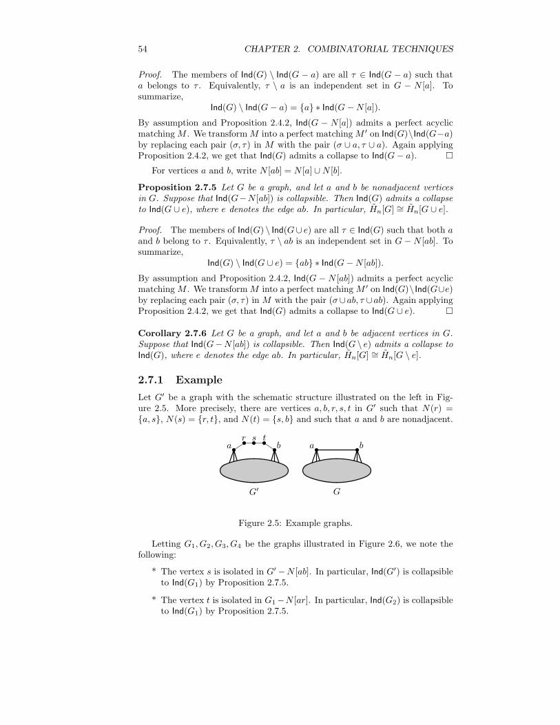
54 CHAPTER 2. COMBINATORIAL TECHNIQUES
Proof. The members of Ind(G) \ Ind(G − a) are all τ ∈ Ind(G − a) such thata belongs to τ . Equivalently, τ \ a is an independent set in G − N [a]. Tosummarize,
Ind(G) \ Ind(G− a) = {a} ∗ Ind(G−N [a]).
By assumption and Proposition 2.4.2, Ind(G − N [a]) admits a perfect acyclicmatching M . We transformM into a perfect matchingM ′ on Ind(G)\Ind(G−a)by replacing each pair (σ, τ) in M with the pair (σ ∪ a, τ ∪ a). Again applyingProposition 2.4.2, we get that Ind(G) admits a collapse to Ind(G− a). �
For vertices a and b, write N [ab] = N [a] ∪N [b].
Proposition 2.7.5 Let G be a graph, and let a and b be nonadjacent verticesin G. Suppose that Ind(G−N [ab]) is collapsible. Then Ind(G) admits a collapseto Ind(G ∪ e), where e denotes the edge ab. In particular, Hn[G] ∼= Hn[G ∪ e].
Proof. The members of Ind(G) \ Ind(G∪ e) are all τ ∈ Ind(G) such that both aand b belong to τ . Equivalently, τ \ ab is an independent set in G−N [ab]. Tosummarize,
Ind(G) \ Ind(G ∪ e) = {ab} ∗ Ind(G−N [ab]).
By assumption and Proposition 2.4.2, Ind(G − N [ab]) admits a perfect acyclicmatching M . We transformM into a perfect matching M ′ on Ind(G)\ Ind(G∪e)by replacing each pair (σ, τ) in M with the pair (σ∪ab, τ ∪ab). Again applyingProposition 2.4.2, we get that Ind(G) admits a collapse to Ind(G ∪ e). �
Corollary 2.7.6 Let G be a graph, and let a and b be adjacent vertices in G.Suppose that Ind(G−N [ab]) is collapsible. Then Ind(G \ e) admits a collapse toInd(G), where e denotes the edge ab. In particular, Hn[G] ∼= Hn[G \ e].
2.7.1 Example
Let G′ be a graph with the schematic structure illustrated on the left in Fig-ure 2.5. More precisely, there are vertices a, b, r, s, t in G′ such that N(r) ={a, s}, N(s) = {r, t}, and N(t) = {s, b} and such that a and b are nonadjacent.
a br s t
G′
a br s t
G
Figure 2.5: Example graphs.
Letting G1, G2, G3, G4 be the graphs illustrated in Figure 2.6, we note thefollowing:
* The vertex s is isolated in G′ −N [ab]. In particular, Ind(G′) is collapsibleto Ind(G1) by Proposition 2.7.5.
* The vertex t is isolated in G1−N [ar]. In particular, Ind(G2) is collapsibleto Ind(G1) by Proposition 2.7.5.

2.7. INDEPENDENCE COMPLEXES 55
a br s t
G1
a br s t
G2
a br s t
G3
a br s
G4
Figure 2.6: More example graphs.
* The vertex r is isolated in G2 −N [tb]. In particular, Ind(G3) is collapsibleto Ind(G2) by Proposition 2.7.5.
* The vertex r is also isolated in G3 − N [t]. In particular, Ind(G3) is col-lapsible to Ind(G4) by Proposition 2.7.4.
We conclude that
Hn[G′] ∼= Hn[G1] ∼= Hn[G2] ∼= Hn[G3] ∼= Hn[G4]
for all n.Now, G4 is the disjoint sum of K2 and G, where G is the graph illustrated
on the right in Figure 2.5. In particular, Proposition 2.7.3 yields that
Hn[G4] ∼= Hn−1[G]
for all n. To summarize, we have that
Hn[G′] ∼= Hn−1[G] (2.8)
for all n.For example, let G′ be the cycle graph Ok. This is the graph with vertex
set {1, . . . , k} and edge set {12, 23, 34, . . . , (k − 1)k, 1k}. Assume that k ≥ 6.Choosing (a, r, s, t, b) = (1, k, k − 1, k − 2, k − 3) and writing e = ab, we notethat
G = (Ok − {r, s, t}) ∪ e = Ok−3.
In particular,Hn[Ok] ∼= Hn−1[Ok−3].
Examining Ind(Ok) by hand for k ≤ 5 and using induction on k, we obtain thatHn[Ok] is zero for all n and k, except that
Hk−1[O3m] ∼= F2,
Hk[O3m+1] ∼= F,
Hk[O3m+2] ∼= F,
for all m ≥ 1.Let us give a second method for deriving the identity (2.8). We may divide
Ind(G′) into the following families:
* The family F∅ of graphs not containing a and b;
F∅ = {∅, r, s, t, rt} ∗ Ind(G− {a, b}).
56 CHAPTER 2. COMBINATORIAL TECHNIQUES
* The family Fa of graphs containing a but not b;
Fa = {a, as, at} ∗ Ind(G−N [a] ∪ {b}).
* The family Fb of graphs containing b but not a;
Fb = {b, br, bs} ∗ Ind(G− {a} ∪N [b]).
* The family Fab of graphs containing both a and b;
Fab = {ab, abs} ∗ Ind(G−N [ab]) = Ind(G′) \ Ind(G1),
where G1 is the graph on the left in Figure 2.6.
We obtain a collapse from Ind(G′) to Ind(G1) by forming the matching
Mab = {(ab, abs)} ∗ Ind(G−N [ab]);
we use the notation in (2.7). Namely, this is a perfect matching on Fab, and thematching is acyclic by Proposition 2.6.1.
By Corollary 2.4.5, we obtain an acyclic matching on Ind(G1) by taking theunion of any acyclic matchings on the families F∅, Fa, and Fb. Let us pick thematchings
M∅ = {(∅, r), (t, rt)} ∗ Ind(G− {a, b}),
Ma = {(a, at)} ∗ Ind(G−N [a] ∪ {b}),
Mb = {(b, br)} ∗ Ind(G− {a} ∪N [b]).
By Proposition 2.6.1, each of these matchings is acyclic. In particular, the unionM = M∅ ∪Ma ∪Mb is acyclic.
Note that M is a perfect matching on delInd(G1)(s) = Ind(G1 − s) and thatthe family of unmatched faces is
{s} ∗ linkInd(G1)(s) = {s} ∗ Ind(G1 −N [s]) = {s} ∗ Ind(G).
Since Hn[G1 − s] = 0 for all n, we may apply Proposition 2.6.4 to obtain (2.8).
Chapter 3
Algebraic techniques
3.1 Exact sequences
One of the most important concepts in mathematics is that of an exact chaincomplex. In such a complex
C : · · ·dn+2
−−−−→ Cn+1dn+1
−−−−→ Cndn−−−−→ Cn−1
dn−1
−−−−→ · · · ,
every cycle is a boundary. Equivalently,
Zn(C) = Bn(C)
for every n. One typically refers to exact chain complexes as (long) exact se-quences. The word “long” means that the sequence extends indefinitely in bothdirections; we have a chain group Cn defined for every n ∈ Z. There is also theconcept of a short exact sequence. This is a sequence involving only five groups,the very first and the very last being zero;
0 −−−−→ Ai
−−−−→ Bs
−−−−→ C −−−−→ 0.
The sequence being exact means that i : A → B is injective, s : B → C issurjective, and im i = ker s. More generally, we have the following result.
Proposition 3.1.1 Suppose we have an exact sequence of F-modules
A : · · ·dn+2
−−−−→ An+1dn+1
−−−−→ Andn−−−−→ An−1
dn−1
−−−−→ · · · .
Then the following hold.
• If dn+1 = 0, then dn : An → An−1 is injective.
• If dn−1 = 0, then dn : An → An−1 is surjective.
In particular, dn : An → An−1 is an isomorphism if dn+1 and dn−1 are bothzero maps.
Proof. The homomorphism dn is injective if and only if kerdn = 0, and dn issurjective if and only if im dn = An−1. Now, if dn+1 = 0, then 0 = im dn+1 =ker dn. Moreover, if dn−1 = 0, then An−1 = ker dn−1 = im dn. For the final
57

58 CHAPTER 3. ALGEBRAIC TECHNIQUES
statement, a homomorphism is an isomorphism if and only if it is injective andsurjective. �
There is an entire area of mathematics – homological algebra – devoted tothe study of exact sequences and their relatives. Since a chain complex C isexact if and only if Hn(C) is zero for every n, one may view the homology of Cas a measure on how far C is from being exact.
3.2 Chain maps and chain isomorphisms
Another important concept is that of isomorphic chain complexes. Intuitively,two chain complexes are isomorphic if it is possible to identify the chain groupsof the two complexes in a way compatible with the boundary maps.
Let
X : · · ·fn+2
−−−−→ Xn+1fn+1
−−−−→ Xnfn
−−−−→ Xn−1fn−1
−−−−→ · · ·
Y : · · ·gn+2
−−−−→ Yn+1gn+1
−−−−→ Yngn
−−−−→ Yn−1gn−1
−−−−→ · · ·
be two chain complexes. A chain map ϕ : X → Y is a sequence (ϕn : n ∈ Z) ofF-module homomorphisms ϕn : Xn → Yn such that
ϕn−1 ◦ fn = gn−1 ◦ ϕn
for all n. This means that the following diagram commutes:
· · ·fn+2
−−−−→ Xn+1fn+1
−−−−→ Xnfn
−−−−→ Xn−1fn−1
−−−−→ · · ·
ϕn+1
y ϕn
y ϕn−1
y
· · ·gn+2
−−−−→ Yn+1gn+1
−−−−→ Yngn
−−−−→ Yn−1gn−1
−−−−→ · · ·
Equivalently, the result when going from Xn to Yn−1 does not depend onwhether we go first right and then down or first down and then right. Notethat ϕn induces a homomorphism
ϕ∗n : Hn(X) → Hn(Y).
Namely, if x ∈ ker fn, then
0 = ϕn−1fn(x) = gnϕn(x) =⇒ ϕn(x) ∈ ker gn.
Moreover, if x ∈ im fn+1, meaning that x = fn+1(x′) for some x′ ∈ Xn+1, then
ϕn(x) = ϕnfn+1(x′) = gn+1(ϕn+1(x
′)) =⇒ ϕn(x) ∈ im gn+1.
We say that a chain map ϕ is a chain isomorphism if every ϕn is an isomor-phism.
Proposition 3.2.1 With notation as above, suppose that ϕ is a chain isomor-phism, and let n ∈ Z. Then ϕn induces an isomorphism
ϕ∗n : Hn(X) → Hn(Y)
for each n.
3.3. RELATIVE HOMOLOGY 59
Proof. We have that
ϕn(ker fn) = ϕn(kerϕn−1fn) = ϕn(ker gnϕn) = ker gn,
because ϕn−1 is injective and ϕn is surjective. As a consequence, ϕ∗n is surjective;
for every y ∈ ker gn, there is an x ∈ ker fn such that ϕ∗n(x + im fn+1) = y +
im gn+1. Moreover,
ϕn(im fn+1) = gn+1(ϕn+1(Xn+1)) = gn+1(Yn+1) = im gn+1,
because ϕn+1 is surjective. In particular, x ∈ im fn if and only if ϕn(x) ∈ im gn,because ϕn is injective. We deduce that ϕ∗
n is injective; ϕ∗n(x+ im fn+1) is zero
if and only x ∈ im fn+1. �
3.3 Relative homology
Let C be a chain complex, and let C(0) be a subcomplex of C. We define therelative chain complex
Q : · · ·dn+2
−−−−→ Qn+1dn+1
−−−−→ Qndn−−−−→ Qn−1
dn−1
−−−−→ · · ·
of the pair (C,C(0)) in the following manner. The nth chain group of Q is definedto be the quotient
Qn =Cn
C(0)n
.
The boundary map dn : Qn → Qn−1 is the one induced by dn : Cn → Cn−1.Specifically,
dn(x+ C(0)n ) = dn(x) + C
(0)n−1.
This is well-defined, because dn(C(0)n ) ⊆ C
(0)n−1. We let Hn(C,C(0)) denote the
homology in degree n of Q and refer to it as the relative homology of the pair(C,C(0)).
For a simplicial complex ∆ and a subcomplex ∆0, let C(∆,∆0; F) denotethe relative chain complex of the pair (C(∆; F),C(∆0; F)). For convenience, wewrite
Hn(∆,∆0; F) = Hn(C(∆; F),C(∆0; F)).
We refer to this as the relative homology of the pair (∆,∆0).The situation is particularly nice for simplicial complexes. Specifically, we
may identify the quotient Cn(∆; F)/Cn(∆0; F) with the submodule of Cn(∆; F)generated by all oriented simplices corresponding to faces of dimension n in∆ \ ∆0. We obtain the boundary ∂n(c) by computing the ordinary boundary∂n(c) and removing all oriented simplices corresponding to faces of ∆0.
Running example 1. Let 2V be the full simplex on the vertex set V = {a, b, c, d}.Then 2V \ E1 is the family {ad, abd, acd, bcd, abcd}. In particular,
C3(2V , E1; F) ∼= 〈abcd〉 ∼= F,
C2(2V , E1; F) ∼= 〈abd, acd, bcd〉 ∼= F3,
C1(2V , E1; F) ∼= 〈ad〉 ∼= F.

60 CHAPTER 3. ALGEBRAIC TECHNIQUES
For n /∈ {1, 2, 3}, we have that Cn(2V , E1; F) = 0. The boundary maps are definedby
∂2(abd) = −ad,
∂3(abcd) = bcd− acd+ abd, ∂2(acd) = −ad, ∂1(ad) = 0.
∂2(bcd) = 0,
For example, abc does not appear in the boundary of abcd, because abc ∈ E1.
Formally, write T = ∆\∆0, and let Pn be the submodule of Cn(∆) generatedby oriented simplices in T of dimension n. We may write Cn(∆) = Cn(∆0)⊕Pn.In particular,
Cn(∆)
Cn(∆0)=Cn(∆0) ⊕ Pn
Cn(∆0) ⊕ 0∼=Cn(∆0)
Cn(∆0)⊕Pn
0∼= Pn;
here, we use Proposition 0.2.1. The reader may check that an isomorphismϕn : Pn → Cn(∆)/Cn(∆0) is given by
ϕn(p) = p+ Cn(∆0).
Define ∂n : Pn → Pn−1 by ∂n(p) = p0, where p0 is the unique element in Pn−1
such that p0 − ∂n(p) ∈ Cn−1(∆0). Then
ϕn−1∂n(p) = p0 + Cn−1(∆0)
= ∂n(p) + (p0 − ∂n(p)) + Cn−1(∆0)
= ∂n(p) + Cn−1(∆0) = ∂n(p+ Cn(∆0)) = ∂nϕn(p).
In particular, C(∆,∆0; F) is isomorphic to the chain complex
P(∆,∆0) : · · ·∂n+2
−−−−→ Pn+1∂n+1
−−−−→ Pn∂n−−−−→ Pn−1
∂n−1
−−−−→ · · ·
It is clear from the above procedure that the chain complex P(∆,∆0) onlydepends on ∆ \ ∆0, not on the particular choice of ∆ and ∆0. Specifically, if∆\∆0 = Γ\Γ0, then P(∆,∆0) = P(Γ,Γ0). To summarize, we have the followingresult.
Proposition 3.3.1 Let Γ and ∆ be simplicial complexes, let Γ0 be a subcomplexof Γ, and let ∆0 be a subcomplex of ∆. If Γ \Γ0 = ∆ \∆0, then C(Γ,Γ0; F) andC(∆,∆0; F) are isomorphic. In particular,
Hn(Γ,Γ0; F) ∼= Hn(∆,∆0; F)
for all n.
For the final statement, apply Proposition 3.2.1.Return to the general case. In what follows, a crucial observation is that
there exists a mapd∗n : Hn(C,C(0)) → Hn(C(0)).
This map sends the homology class of an element x+C(0)n ∈ Zn(C,C(0)) to the
homology class of the element dn(x) ∈ Zn−1(C(0)). This is well-defined, because
if c ∈ C(0)n , then
dn(x+ c) − dn(x) = dn(c) ∈ Bn−1(C(0));
3.3. RELATIVE HOMOLOGY 61
hence dn(x) and dn(x+ c) belong to the same homology class.Note that elements in im d∗n are not necessarily zero. Specifically, an element
y ∈ C(0)n−1 might be a boundary of some element in Cn without being a boundary
of any element in C(0)n .
The following theorem is one of the most important results in homologicalalgebra. The long exact sequence in the theorem is known as the long exactsequence for the pair (C,C(0)).
Theorem 3.3.2 For any chain complex C and any subcomplex C(0) of C, wehave the following long exact sequence.
· · ·i∗n+1
−−−−→ Hn+1(C)s∗
n+1
−−−−→ Hn+1(C,C(0))
d∗
n+1
−−−−→d∗
n+1
−−−−→ Hn(C(0))i∗n−−−−→ Hn(C)
s∗
n−−−−→ Hn(C,C(0))d∗
n−−−−→
d∗
n−−−−→ Hn−1(C(0))
i∗n−1
−−−−→ Hn−1(C)s∗
n−1
−−−−→ · · ·
The map i∗n is induced by the inclusion map in : C(0)n → Cn, the map s∗n is
induced by the projection map sn : Cn → Cn/C(0)n , and the map d∗n is defined
above.
Proof. Write C(1) = C. For x ∈ Zn(C(i)) and i ∈ {0, 1}, let [x]i denote the
homology class of x in Hn(C(i)). For x + C(0)n ∈ Zn(C(1),C(0)), let [x]2 denote
the homology class of x+ C(0)n in Hn(C(1),C(0)).
First, we prove that im i∗n = ker s∗n. We note that [x]1 belongs to im i∗n ifand only if there is an element x′ ∈ Zn(C(0)) such that x− x′ ∈ Bn(C(1)). As aconsequence, s∗ni
∗n is zero, because s∗n maps [x]1 to
[x]2 = [x− x′]2 + [x′]2 = [0]2.
Conversely, if [x]1 ∈ ker s∗n, then x − d(y) ∈ C(0)n for some y ∈ C
(1)n+1. Writing
x′ = x − d(y), we note that x′ ∈ Zn(C(0)) and x − x′ ∈ Bn(C(1)); hence [x]1 =[x′]1 ∈ im i∗n.
Second, we prove that im s∗n = ker d∗n. We note that [x]2 belongs to im s∗nif and only if there is an element x′ ∈ Zn(C(1)) such that x − x′ ∈ C(0). As aconsequence, d∗ns
∗n is zero, because d∗n maps [x]2 to
[dn(x)]0 = [dn(x− x′)]0 + [dn(x′)]0 = [0]0.
Conversely, if [x]2 ∈ kerd∗n, then dn(x) = dn(x(0)) for some x(0) ∈ C(0)n . Writing
x′ = x− x(0), we note that x′ ∈ Zn(C(1)) and x− x′ ∈ C(0); hence [x]2 = [x′]2 ∈im s∗n.
Third, we prove that im d∗n = ker i∗n−1. We note that [x]0 belongs to im d∗n if
and only if there is an element y ∈ Cn(C(1)) such that x− dn(y) ∈ Bn−1(C(0)).
As a consequence, i∗n−1d∗n is zero, because i∗n−1 maps [x]0 to
[x]1 = [x− dn(y)]1 + [dn(y)]1 = [0]1.
Conversely, if [x]0 ∈ ker i∗n, then x = dn(y) for some y ∈ C(1)n ; hence [x]2 ∈ im s∗n.
�

62 CHAPTER 3. ALGEBRAIC TECHNIQUES
Corollary 3.3.3 The following hold for any integer n.
(i) If Hn(C(0)) = Hn−1(C(0)) = 0, then Hn(C) ∼= Hn(C,C(0)).
(ii) If Hn(C) = Hn−1(C) = 0, then Hn−1(C(0)) ∼= Hn(C,C(0)).
(iii) If Hn+1(C,C(0)) = Hn(C,C(0)) = 0, then Hn(C) ∼= Hn(C(0)).
Proof.
(i) Suppose thatHn(C(0)) = Hn−1(C(0)) = 0. Then we get the exact sequence
0i∗n−−−−→ Hn(C)
s∗
n−−−−→ Hn(C,C(0))d∗
n−−−−→ 0.
In particular, Hn(C) ∼= Hn(C,C(0)).
(ii) Suppose that Hn(C) = Hn−1(C) = 0. Then we get the exact sequence
0s∗
n−−−−→ Hn(C,C(0))d∗
n−−−−→ Hn−1(C(0))
i∗n−1
−−−−→ 0.
In particular, Hn−1(C(0)) ∼= Hn(C,C(0)).
(iii) Suppose that Hn+1(C,C(0)) = Hn(C,C(0)) = 0. Then we get the exact
sequence
0d∗
n+1
−−−−→ Hn(C(0))i∗n−−−−→ Hn(C)
s∗
n−−−−→ 0.
In particular, Hn(C) ∼= Hn(C(0)).
�
Corollary 3.3.4 For any simplicial complex ∆ and any subcomplex ∆0 of ∆,we have the following long exact sequence.
· · ·i∗n+1
−−−−→ Hn+1(∆)s∗
n+1
−−−−→ Hn+1(∆,∆0)∂∗
n+1
−−−−→∂∗
n+1
−−−−→ Hn(∆0)i∗n−−−−→ Hn(∆)
s∗
n−−−−→ Hn(∆,∆0)∂∗
n−−−−→
∂∗
n−−−−→ Hn−1(∆0)i∗n−1
−−−−→ Hn−1(∆)s∗
n−1
−−−−→ · · ·
The map i∗n is induced by the inclusion map in : Cn(∆0) → Cn(∆), the map s∗nis induced by the projection map sn : Cn(∆) → Cn(∆)/Cn(∆0), and the map∂∗n is defined in the same manner as d∗n in Theorem 3.3.2.
Corollary 3.3.5 The following hold for any integer n.
(i) If Hn(∆0; F) = Hn−1(∆0; F) = 0, then Hn(∆; F) ∼= Hn(∆,∆0; F).
(ii) If Hn(∆; F) = Hn−1(∆; F) = 0, then Hn−1(∆0; F) ∼= Hn(∆,∆0; F).
(iii) If Hn+1(∆,∆0; F) = Hn(∆,∆0; F) = 0, then Hn(∆; F) ∼= Hn(∆0; F).
Let 2V be a k-simplex; k = |V | − 1. We obtain the boundary of a k-simplexby removing the maximal face V from 2V .
3.4. MAYER-VIETORIS SEQUENCES 63
Corollary 3.3.6 If Σ is the boundary of a k-simplex, then
Hn(Σ; F) ∼=
{F if n = k − 1,0 otherwise.
Proof. Let ∆ be the full k-simplex 2V ; we have that V has size k + 1. Then∆ \ Σ consists of one single simplex of dimension k. As a consequence,
Hn(∆,Σ; F) ∼=
{F if n = k,0 otherwise.
Now, Hn(∆; F) = 0 for all n by Corollary 2.3.4. As a consequence, Hn−1(Σ; F) ∼=Hn(∆,Σ; F) by Corollary 3.3.5 (ii), which yields the desired result. �
For any simplicial complex ∆1 and any subcomplex ∆0, it is easy to constructa simplicial complex ∆2 with the same homology as the pair (∆1,∆0).
Corollary 3.3.7 Let ∆1 be a simplicial complex, and let ∆0 be a subcomplexof ∆1. Let a be a vertex not in ∆1. Define
∆2 = Conea(∆0) ∪ ∆;
this is the simplicial complex obtained from ∆1 by adding σ∪a for each σ ∈ ∆0.Then
Hn(∆2; F) ∼= Hn(∆1,∆0; F).
Proof. By Proposition 2.3.3, we have that Conea(∆0) is collapsible. As aconsequence,
Hn(∆2; F) ∼= Hn(∆2,Conea(∆0); F).
Yet, ∆2 \ Conea(∆0) = ∆1 \ ∆0, which implies that
Hn(∆2,Conea(∆0)) ∼= Hn(∆1,∆0).
As a consequence, we obtain the desired result. �
Note that ∆1 = del∆2(a) and ∆0 = link∆2
(a). In the case that Hn(∆1) = 0for all n, we recover Proposition 2.6.4. Namely,
Hn(∆2) ∼= Hn(∆1,∆0) ∼= Hn−1(∆0) = Hn−1(link∆2(a))
by Corollary 3.3.7 and Corollary 3.3.5 (ii).
3.4 Mayer-Vietoris sequences
In Section 3.3, we related the homology of a complex C to the homology of asubcomplex C(0) via a long exact sequence involving the relative homology of thepair (C,C(0)). In this section, we discuss another long exact sequence relatingthe homology of two subcomplexes of the same complex to the homology oftheir sum and intersection.
Let
X : · · ·dn+2
−−−−→ Xn+1dn+1
−−−−→ Xndn−−−−→ Xn−1
dn−1
−−−−→ · · ·
Y : · · ·dn+2
−−−−→ Yn+1dn+1
−−−−→ Yndn−−−−→ Yn−1
dn−1
−−−−→ · · ·

64 CHAPTER 3. ALGEBRAIC TECHNIQUES
be subcomplexes of the same complex C. Let X+Y be the subcomplex of C withchain groups Xn +Yn. Moreover, let X∩Y be the subcomplex with chain groupsXn ∩ Yn. One easily checks that these are indeed chain complexes. The longexact sequence in the following theorem is known as a Mayer-Vietoris sequence.
Theorem 3.4.1 With notation as above, we have a long exact sequence
· · ·f∗
n+1
−−−−→ Hn+1(X ⊕ Y)g∗
n+1
−−−−→ Hn+1(X + Y)h∗
n+1
−−−−→h∗
n+1
−−−−→ Hn(X ∩ Y)f∗
n−−−−→ Hn(X ⊕ Y)g∗
n−−−−→ Hn(X + Y)h∗
n−−−−→
h∗
n−−−−→ Hn−1(X ∩ Y)f∗
n−1
−−−−→ Hn−1(X ⊕ Y)g∗
n−1
−−−−→ · · ·
The map f∗n is induced by the map fn : Cn(X ∩ Y) → Cn(X ⊕ Y) given by
fn(s) = (s,−s). The map g∗n is induced by the map gn : Cn(X⊕Y) → Cn(X+Y)given by gn(x, y) = x+ y. The map h∗n is given by mapping the homology classof z to that of dn(x), where x is any element in Xn such that z − x ∈ Yn.
Remark. Recall from Theorem 2.2.2 that
Hn(X ⊕ Y) ∼= Hn(X) ⊕Hn(Y).
Proof. We may identify X ∩ Y with a certain subcomplex of X ⊕ Y. Namely,
let W be the subcomplex with chain groups
Wn = {(s,−s) : s ∈ Xn ∩ Yn}.
We leave it to the reader to check that we obtain a chain isomorphism ϕ :X∩Y → W defined by ϕn(s) = (s,−s) for all s ∈ Xn∩Yn. Theorem 3.3.2 yieldsa long exact sequence
· · ·i∗n+1
−−−−→ Hn+1(X ⊕ Y)s∗
n+1
−−−−→ Hn+1(X ⊕ Y,W)d∗
n+1
−−−−→d∗
n+1
−−−−→ Hn+1(W)i∗n−−−−→ Hn(X ⊕ Y)
s∗
n−−−−→ Hn(X ⊕ Y,W)d∗
n−−−−→
d∗
n−−−−→ Hn−1(W)i∗n−1
−−−−→ Hn−1(X ⊕ Y)s∗
n−1
−−−−→ · · ·
Now, let Q denote the relative chain complex of the pair (X ⊕ Y,W). We claimthat we obtain a chain isomorphism
ψ : Q → X + Y
byψn((x, y) +Wn) = x+ y
for any x ∈ X and y ∈ Y . The map ψn is well-defined, because if (x′, y′) −(x, y) ∈Wn, then x′ − x+ y′ − y = 0, which yields that
x′ + y′ = x+ y + (x′ − x+ y′ − y) = x+ y.
Moreover, ψn is injective, because ψn((x, y) +Wn) = 0 if and only if y = −x,which is equivalent to saying that (x, y) ∈ Wn. Finally, ψn is surjective, becauseany element in Xn+Yn is of the form x+y = ψn((x, y)+Wn). As a consequence,

3.5. INDEPENDENCE COMPLEXES REVISITED 65
we get a long exact sequence as in the theorem, and it only remains to showthat f∗
n, g∗n, and h∗n are as specified there.Now, f∗
n is induced by inϕn, and
inϕn(s) = in(s,−s) = (s,−s) = fn(s).
Moreover, g∗n is induced by ψnsn, and
ψnsn(x, y) = ψn((x, y) +Wn) = x+ y = gn(x, y).
Finally, h∗n maps the homology class of an element x + y = ψn((x, y) +Wn) ∈ker dn to the homology class of
ϕ−1n (dn(x), dn(y)) = ϕ−1
n (dn(x),−dn(x)) = dn(x).
This concludes the proof. �
Let ∆ and Γ be simplicial complexes. We note that
C(∆; F) ∩ C(Γ; F) = C(∆ ∩ Γ; F),
C(∆; F) + C(Γ; F) = C(∆ ∪ Γ; F).
In particular, we have the following result.
Corollary 3.4.2 With notation as above, we have a long exact sequence
· · ·f∗
n+1
−−−−→ Hn+1(∆) ⊕ Hn+1(Γ)g∗
n+1
−−−−→ Hn+1(∆ ∪ Γ)h∗
n+1
−−−−→ Hn(∆ ∩ Γ)f∗
n−−−−→ Hn(∆) ⊕ Hn(Γ)g∗
n−−−−→ Hn(∆ ∪ Γ)
h∗
n−−−−→ Hn−1(∆ ∩ Γ)f∗
n−1
−−−−→ Hn−1(∆) ∪ Hn−1(Γ)g∗
n−1
−−−−→ · · ·
The maps f∗n, g∗n, and h∗n are defined as in Theorem 3.4.1.
3.5 Independence complexes revisited
Recall definitions and concepts from Section 2.7. As before, we write Hn[G] =Hn(Ind(G); F), and we also write Cn[G] = Cn(Ind(G); F). One may view Theo-rems 3.5.1 and 3.5.4 as algebraic generalizations of Propositions 2.7.4 and 2.7.5.
Theorem 3.5.1 Let G be a graph, and let a be a vertex in G. Then we havethe following long exact sequence.
· · ·i∗n+1
−−−−→ Hn+1[G]t∗n+1
−−−−→ Hn[G−N [a]]j∗n−−−−→
j∗n−−−−→ Hn[G− a]
i∗n−−−−→ Hn[G]
t∗n−−−−→ Hn−1[G−N [a]]
j∗n−1
−−−−→
j∗n−−−−→ Hn−1[G− a]
i∗n−1
−−−−→ Hn−1[G]t∗n−1
−−−−→ · · ·
The maps i∗n and j∗n are induced by the inclusion maps in : Cn[G− a] → Cn[G]and jn : Cn[G−N [a]] → Cn[G− a]. The map t∗n is induced by the map tn :Cn[G] → Cn−1[G−N [a]] given by tn(x+a∧y) = y for each x ∈ Cn[G− a] andy ∈ Cn−1[G−N [a]].
66 CHAPTER 3. ALGEBRAIC TECHNIQUES
Proof. Consider the long exact sequence for the pair (Ind(G), Ind(G− a)). Asconcluded in the proof of Proposition 2.7.4,
Ind(G) \ Ind(G− a) = {a} ∗ Ind(G−N [a]).
Now, this is equal to
Conea(Ind(G−N [a])) \ Ind(G−N [a]).
As a consequence, Proposition 3.3.1 and Corollary 2.6.5 yield that
Hn(Ind(G), Ind(G− a)) ∼= Hn(Conea(Ind(G−N [a])), Ind(G−N [a]))∼= Hn−1(Ind(G−N [a]))
= Hn−1[G−N [a]].
By the long exact sequence for the pair (Conea(Ind(G−N [a])), Ind(G−N [a])),we have an isomorphism ϕn from Hn(Ind(G), Ind(G − a)) to Hn−1[G−N [a]]given by mapping the homology class of a∧y+ Cn[G− a] to the homology classof ∂n(a ∧ y) = y. As a consequence, the map t∗n = ϕns
∗n sends the homology
class of x+ a ∧ y to the homology class of y, and the map j∗n = ∂∗n+1ϕ−1n sends
the homology class of y to the homology class of ∂n+1(a ∧ y) = y. �
Corollary 3.5.2 Let G be a graph, and let a be a vertex in G.
(i) If Hn[G− a] = Hn−1[G− a] = 0, then Hn[G] ∼= Hn−1[G−N [a]].
(ii) If Hn+1[G] = Hn[G] = 0, then Hn[G− a] ∼= Hn[G−N [a]].
(iii) If Hn[G−N [a]] = Hn−1[G−N [a]] = 0, then Hn[G] ∼= Hn[G− a].
Corollary 3.5.3 Let G be a graph, and assume that a and b are vertices suchthat a is the only neighbor of b. Then
Hn[G] ∼= Hn−1[G−N [a]]
for all n.
Proof. We have that b is isolated in G− a, which implies that Hn[G− a] = 0for all n. Applying Corollary 3.5.2 (i), we obtain the desired result. �
Example. Let Pk be the path of vertex length k. This is the graph with vertex set{1, . . . , k} and edge set {12, 23, 34, . . . , (k−1)k}. Let k ≥ 3, and choose a = k−1and b = k. Then the conditions of Corollary 3.5.3 are satisfied, which yields that
Hn[Pk] ∼= Hn−1[Pk −N [a]] = Hn−1[Pk−3].
Observing that P0 = {∅}, P1 = {∅, 1}, and P2 = {∅, 1, 2}, a simple inductionargument yields that Hn[Pk] is zero for all n and k, except that
Hm−1[P3m] ∼= Hm[P3m+2] ∼= F
for m ≥ 0.One may also choose a = k − 2, in which case we get that Hn[Pk −N [a]] = 0
for all n. By Corollary 3.5.2 (iii) and Proposition 2.7.3, we conclude that
Hn[Pk] ∼= Hn[Pk − a] = Hn[K2 + Pk−3] ∼= Hn−1[Pk−3].

3.5. INDEPENDENCE COMPLEXES REVISITED 67
Theorem 3.5.4 Let G be a graph, and let a and b be nonadjacent vertices inG. Then we have the following long exact sequence.
· · ·i∗n+1
−−−−→ Hn+1[G]u∗
n+1
−−−−→ Hn−1[G−N [ab]]ℓ∗
n−1
−−−−→ℓ∗
n−1
−−−−→ Hn[G ∪ e]i∗n−−−−→ Hn[G]
u∗
n−−−−→ Hn−2[G−N [ab]]ℓ∗
n−2
−−−−→ℓ∗
n−2
−−−−→ Hn−1[G ∪ e]i∗n−1
−−−−→ Hn−1[G]u∗
n−1
−−−−→ · · ·
Proof. This time, consider the long exact sequence for the pair (Ind(G), Ind(G∪e)). As we concluded in the proof of Proposition 2.7.5,
Ind(G) \ Ind(G ∪ e) = {ab} ∗ Ind(G−N [ab]).
Now, this is equal to
Conea,b(Ind(G−N [ab])) \ Suspa,b(Ind(G−N [ab])),
where Conea,b(∆) = Conea(Coneb(∆)) As a consequence, Proposition 3.3.1,Corollary 3.3.5 (ii), and Corollary 2.6.5 yield that
Hn(Ind(G), Ind(G ∪ a))∼= Hn(Conea,b(Ind(G−N [ab])), Suspa,b(Ind(G−N [ab])))
∼= Hn−1(Suspa,b(Ind(G−N [ab])))
∼= Hn−2(Ind(G−N [ab]))
= Hn−2[G−N [ab]].
This concludes the proof. �
The interested reader may check the following:
• The map i∗n is induced by the inclusion map in : Cn[G ∪ e] → Cn[G].
• The map ℓ∗n is induced by the map ℓn : Cn[G−N [ab]] → Cn+1[G ∪ e]given by ℓn(x) = (b− a) ∧ x.
• The map u∗n is induced by the map un : Cn[G] → Cn−2[G−N [ab]] givenby un(x+ a∧ b∧ y) = y for each x ∈ Cn[G ∪ e] and y ∈ Cn−2[G−N [ab]].
Corollary 3.5.5 Let G be a graph, and let e = ab be an edge not in G.
(i) If Hn[G ∪ e] = Hn−1[G ∪ e] = 0, then Hn[G] ∼= Hn−2[G−N [ab]].
(ii) If Hn+1[G] = Hn[G] = 0, then Hn[G ∪ e] ∼= Hn−1[G−N [ab]].
(iii) If Hn−1[G−N [ab]] = Hn−2[G−N [ab]] = 0, then Hn[G ∪ e] ∼= Hn[G].
Example. Again, consider Pk, and assume that k ≥ 3. Choose a = k − 1 andb = k; write e = ab. We note that k is an isolated vertex in Pk \ e. In particular,Hn[Pk \ e] = 0 for all n. Picking G = Pk \ e in Corollary 3.5.5 (ii), we get that
Hn[Pk] ∼= Hn−1[Pk −N [ab]] = Hn−1[Pk−3].
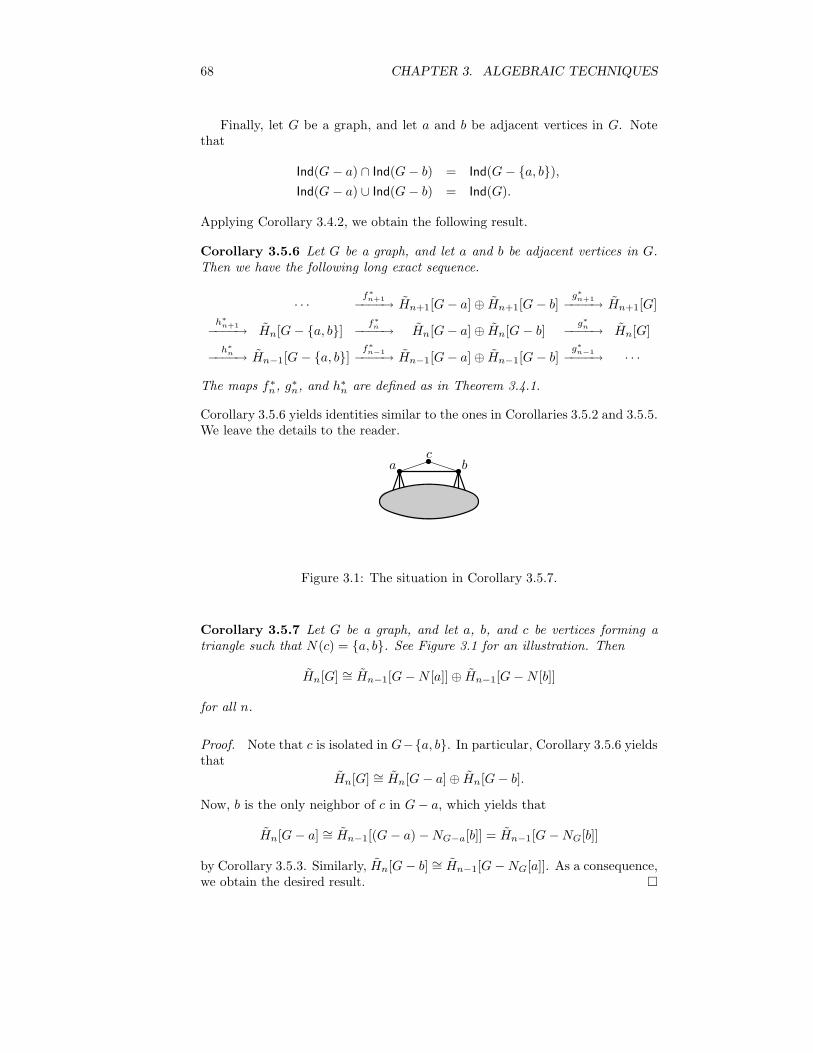
68 CHAPTER 3. ALGEBRAIC TECHNIQUES
Finally, let G be a graph, and let a and b be adjacent vertices in G. Notethat
Ind(G− a) ∩ Ind(G− b) = Ind(G− {a, b}),
Ind(G− a) ∪ Ind(G− b) = Ind(G).
Applying Corollary 3.4.2, we obtain the following result.
Corollary 3.5.6 Let G be a graph, and let a and b be adjacent vertices in G.Then we have the following long exact sequence.
· · ·f∗
n+1
−−−−→ Hn+1[G− a] ⊕ Hn+1[G− b]g∗
n+1
−−−−→ Hn+1[G]h∗
n+1
−−−−→ Hn[G− {a, b}]f∗
n−−−−→ Hn[G− a] ⊕ Hn[G− b]g∗
n−−−−→ Hn[G]
h∗
n−−−−→ Hn−1[G− {a, b}]f∗
n−1
−−−−→ Hn−1[G− a] ⊕ Hn−1[G− b]g∗
n−1
−−−−→ · · ·
The maps f∗n, g∗n, and h∗n are defined as in Theorem 3.4.1.
Corollary 3.5.6 yields identities similar to the ones in Corollaries 3.5.2 and 3.5.5.We leave the details to the reader.
a bc
Figure 3.1: The situation in Corollary 3.5.7.
Corollary 3.5.7 Let G be a graph, and let a, b, and c be vertices forming atriangle such that N(c) = {a, b}. See Figure 3.1 for an illustration. Then
Hn[G] ∼= Hn−1[G−N [a]] ⊕ Hn−1[G−N [b]]
for all n.
Proof. Note that c is isolated in G−{a, b}. In particular, Corollary 3.5.6 yieldsthat
Hn[G] ∼= Hn[G− a] ⊕ Hn[G− b].
Now, b is the only neighbor of c in G− a, which yields that
Hn[G− a] ∼= Hn−1[(G− a) −NG−a[b]] = Hn−1[G−NG[b]]
by Corollary 3.5.3. Similarly, Hn[G− b] ∼= Hn−1[G−NG[a]]. As a consequence,we obtain the desired result. �

3.5. INDEPENDENCE COMPLEXES REVISITED 69
a
b
cde
f
g h
Figure 3.2: Example graph.
Example. Let G be the graph in Figure 3.2. We note that the conditions ofCorollary 3.5.7 are satisfied. Now, G−N [a] is isomorphic to P3, whereas G−N [b]is isomorphic to P5. As a consequence, we get that
Hn[G] ∼= Hn−1[P3] ⊕ Hn−1[P5] ∼=
F if n = 1,F if n = 2,0 otherwise.

70 CHAPTER 3. ALGEBRAIC TECHNIQUES

Bibliography
[1] P. L. Hersh, On optimizing discrete Morse functions, Adv. in Appl. Math.35 (2005), 294–322. European J. Combin. 30 (2009), 429–438.
[2] J. Jonsson, Simplicial Complexes of Graphs, Lecture Notes in Mathematics1928, Springer, 2008.
71


![Simplicial Homology Global Optimisation - A Lipschitz ...In the development ofshgowe require several concepts from algebraic and combinatorial topology [Hatcher, 2002, Henle, 1979]](https://img.dokumen.tips/doc/110x75/5ecfe10a98bf530014195a95/simplicial-homology-global-optimisation-a-lipschitz-in-the-development-ofshgowe.jpg)


![CYCLIC HOMOLOGY ARISING FROM ADJUNCTIONS · the homology of suitable comonads T, de ned via simplicial objects C Tp N;Mq obtained from the bar construction (see, e.g., [Wei94]). Connes’](https://img.dokumen.tips/doc/110x75/6015683185fbeb6c746f0c9a/cyclic-homology-arising-from-adjunctions-the-homology-of-suitable-comonads-t-de.jpg)


