Embed Size (px)
Citation preview

ContentPart A Part B1. Overview of Matlab2. Getting started3. Documentation and help 4. Variables5. Matrix operations6. Built-in functions7. Controlling work flow
8. Basic input/output9. Scripts and functions10. Reading and writing data11. Fitting a model to data12. Solving differential
equations13. Plotting in 2d and 3d
http://www.mathworks.com/academia/student_center/tutorials/launchpad.html www. http://www.stanford.edu/~wfsharpe/mia/mat/mia_mat3.htm
The labs are interactive, computer-based tutorials that offer us the opportunity to go over your exercises, as well as look into some related mathematics. Another good reference is the primer by Kermit Sigmon (pdf) as well as the official Matlab documentation.

1. Overview of Matlab
Intuitive, easy-to-learn, high performance language integrating: computation, visualization, and programming.
• Math and computation• Algorithm development• Data acquisition• Modeling, simulations, and prototyping• Data analysis, exploration, and visualization• Scientific and engineering graphics• Application development, incl. graphical user interfaces
MATLAB stands for matrix laboratory. Its basic variables are arrays, i.e.vectors and matrices. Matlab also has many build-in functions (LAPACK and BLAST libs), as well as specialised add-on tool boxes.Features allow fast implementation of programs to solve computational problems.

The Matlab system consists of 5 main parts:
1. Desktop tools and development environment Mainly graphical user interfaces, editor, debugger, and workspace
2. Mathematical function library Basic math functions such as sums, cosine, complex numbers Advanced math functions such as matrix inversion, matrix eigenvalues, differential equations 3. The language High-level language based on arrays, functions, input/output, and flow statements (for, if, while)
4. Graphics Data plotting in 2d and 3d, as well as image analysis and animation tools
5. External interfaces Interaction between C and Fortran programs with Matlab, either for linking convenient routines from Matlab in C/Fortran, or for Matlab to call fast C/Fortran programs

2. Getting started
Go here to open new or existing Matlab files (M-file) and editor
write Matlab commandshere for interactive mode (work space)
Menus change,depending onthe tool youare using
Enter MATLABstatements atthe prompt
View or changethe currentdirectory

new
existing
Opening new and existing M-files (scripts or M-file functions):

Different ways to use Matlab:
(1) Interactive mode: just type commands and define variables, empty work space with command clear (2) Simple scripts: M-file (name.m) with list of commands Operate on existing data in work space, or create new data to work on Variables remain in workspace (until emptied) Re-useable
(3) Versatile M-file functions: M-file May return values Re-usable Easy to call from other functions (make sure file is in Matlab search path, set by > File > Set Path)

Matlab provides large amounts of documentation and tutorials:3. Documentation and help

Matrix assignment:
4. Variables are represented as matrices
C= A + B assigns matrix C as the sum of matrices A and B
If A and B are matrices of same dimension, e.g. [3x4] with 3 rows and4 columns, C is [3x4] matrix with element-wise addition.
Example with [2x2] matrices:
A= B= C=
If C existed before e.g. was a scalar C=[1] (i.e. a [1x1] matrix), then C isoverwritten by this new assignment.
If dimensions of A and B don’t match, you will get an error:
??? Error using ==> + Matrix dimensions must agree
Matrix variables don’t need to be declared. They are just assigned to values andknow about their dimension.
2 43 7
5 16 2
7 59 9

Showing values:
To see content of a variable, just type its name:
C = A + B provides
To assign a variable without showing its content, use semicolon:
C = A + B; (nothing)
C = 7 5 9 9
Initializing matrices:
Provide initial values, e.g.
a=3; (scalar) b=[ 1 2 3 ]; ([1x3] row vector) c=[ 4 ; 5 ; 6 ]; ([3x1] column vector) d=[ 1 2 3 ; 4 5 6 ]; ([2x3] matrix)
d = 1 2 3 4 5 6
typing d gives
Values separated by spaces are put in the same row, e.g., b=[ 1 2 3 ]Semicolon (or carriage return) separates rows, e.g., c=[ 4 ; 5 ; 6 ]

Making matrices from matrices:
a=[ 1 2 3 ]; b=[ 4 5 6 ]; gives c=[ a b ]; while
a=[ 1 2 3 ]; b=[ 4 5 6 ]; gives c=[ a ; b ];
c = 1 2 3 4 5 6
c = 1 2 3 4 5 6
Using portions of matrices:
d(1,2) returns 2d(2,1) returns 4
d=[ 1 2 3 ; 4 5 6 ]; typing
and d(1, :) returns d(: , 2) returns
1 2 3 2 5
d = 1 2 3 4 5 6

Using more portions of matrices:
d(2,[2 3]) returns 5 6d(2,[3 2]) returns 6 5
d=[ 1 2 3 ; 4 5 6 ]; typing
Variables may also be used as indices of matrices
if you type z = [2 3]then you will see that d(2, z) returns 5 6
Use colon to produce string of consecutive integers
x = 3 : 5 produces vector x = 3 4 5
and d(1, 1:2) returns 1 2
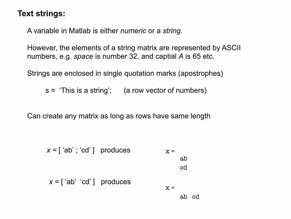
Text strings:
A variable in Matlab is either numeric or a string.
However, the elements of a string matrix are represented by ASCII numbers, e.g. space is number 32, and captial A is 65 etc.
Strings are enclosed in single quotation marks (apostrophes)
s = ‘This is a string’; (a row vector of numbers)
Can create any matrix as long as rows have same length
x = [ ‘ab’ ; ‘cd’ ] produces
x = [ ‘ab’ ‘cd’ ] produces
x = ab cd
x = ab cd

Matrix transposition is obtained by adding a prime (apostrophe)
if x = 1 2 3 (row vector)
then x’ = (column vector) 1 2 3
Matrix addition is obtaind by + sign, and Matrix subtraction is obtained by - sign
If A is a [3x4] matrix and B is a [4x3] matrix, then
C = A + B produces while C = A + B’ works fine
??? Error using ==> + Matrix dimensions must agree
5. Matrix operations

Matrix multiplication is obtained by * symbol
C = A * B
Note that inner dimensions of the two operands must be the same, e.g. A=[3x4] and B=[4x2] works.
Element by element operations are given by
C = A .* B (multiplication)
C = A ./ B (division)
C = A .^ 2 (exponentiation) but for first two, matrix dimensions have to agree!
Exceptions: For addition and subtraction, as well as element-by-element multiplication and division, matrix dimensions can be different if one of theoperand is a scalar. In this case, the scalar is applied to each element in the matrix.

Some provide one, others more than one answer.
Examples: sum, max, and plot functions
if x = 1 2 3
then statement y = sum(x) + 10
produces y = 16
if x = 1 4 3
then statement [y n]= max(x)
produces y = 4 n = 2
if x = 1 4 3
then statement z = 10 + max(x)
produces z = 14
multipleassignmentspossible aswell
position where found
6. Built-in functions value=sum(arg_1,arg_2)
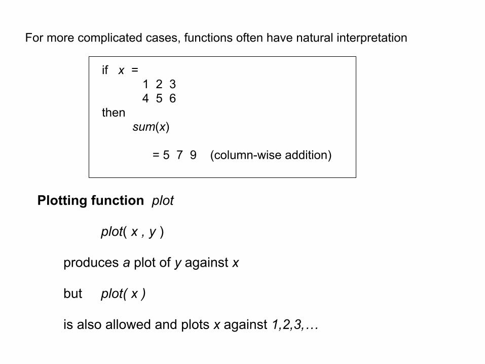
if x = 1 2 3 4 5 6then sum(x) = 5 7 9 (column-wise addition)
For more complicated cases, functions often have natural interpretation
Plotting function plot
plot( x , y )
produces a plot of y against x
but plot( x ) is also allowed and plots x against 1,2,3,…

Other built-in functions are: mean, cov, min, max, ones, zeros, size, rand, randn ….
M-file functions: provided in \matlab\toolbox or written by yourself filename.m
What do built-in or M-file functions do? To obtain description: help mean To see code: type mean
if x = 1 5 3 2 2 8then y = sort( x ) produces y = 1 2 2 5 3 8 i.e., each column is sorted separately
Example: sorting function sort
To obtain a record of the rows from which the sorted elements came:
[y r] = sort( x ) produces y as before and r = 1 2 3 1 2 3

Relational and logical operations:
Matlab knows six relational operations
< less than <= less than or equal to > greater than >= greater than or equal to == equal ~= not equal
and the following logical operators & and | or ~ not
Note:
A=B assigns to A the values of B
(A==B) tests whether A and B areequal

Whenever Matlab encounters a relational operator, it produces a 1 if the expressionis true and a 0 if the expression is false:
x = (1 < 3) produces x=1, whilex = (1 > 3) produces x=0
Relational operators can also be applied to matrices as long as they have thesame dimension (as relational operators then work on an element-by-element basis):
if A = 1 2 3 4and B = 3 1 2 2then C = (A > B) produces C = 0 1 1 1
if A = 1 2 3 4then C = (A > 2) produces C = 0 0 1 1
scalar

To change to a non-sequential order, use for and while loops, as well asif statements
for loops: for j = 1 : n ….. endwhile loops: while (x > 0.5) …… end
For clarity, introduce TRUE and FALSE variables
true = (1==1); false = (1==0); ….. done = false; while not done ….. end
Note: avoid infinite loops by including termination condition
7. Controlling work flow

if statement: if (x > 0.5) if (x > 0.5) ….. or ….. end else …. endNesting: for j = 1 : n for k = 1 : n (indentations are for clarity only) if (x( j , k ) > 0.5) x( j , k ) = 1.5; end end end
Nesting should be avoided for matrix operations, since very slow:
instead of use port_val = holdings * prices ; port_val = 0; for j = 1 : n port_val = port_val + ( holdings(j) * prices(j) ); end

Basic data input: 1. Type instructions in interactive mode or in script mode.
Examples: radius = [ 12.50 37.875 12.25 ]
molecules = [ ‘sugars’ ; ‘amino acids’ ; ‘proteins’ ]
data = [ 100 200
300 400 ] (line breaks for increased clarity)
2. Read text file and put in matrix test: load test.txt
Basic data output: 1. Display data: disp (‘test’);
2. Dump stuff from display into file: diary filename to start and diary off to stop
3. Save data from a matrix, use save newdata.txt test -ascii
4. Save variables etc. from interactive Matlab session in .mat file, use
save temp (saves complete session in temp.mat file)
save temp radius molecules data (saves only certain variables in temp.mat)
load temp (restores session later)
8. Basic input/output

9. Scripts and functionsExample script:An M-file called magicrank.m may contain following code
Typing magicrank executes script, and computes rank of first 30 magic squares and plots bar chart of results

Functions have the advantage that they can be re-used in different programs.A function starts with a line declaring the function, its arguments and its outputs.
Examples:
function y = port_val(holdings, prices) y = holdings * prices;
This function is called by
v = port_val( h, p );
local variables
variables can be named differently in calling statement
function [total_val , avg_val] = port_val(holdings, prices) total_val = holdings * prices; avg_val = total_val/size( holdings , 2 );
This function is called by
[tval aval ] = port_val( h, p );
returnsone value
returnstwo values
Example function:
must be saved in port_val.m

Functions:Name of M-file and function should be the same. Variables only defined in function, not common workspace.
M-file rank.m is available in directory
To see file, write , which produces
To get info, i.e., first lines of comments (starting with %), write
Function can be called as

Anonymous functions:
Primary and subfunctions:
Function handles:
Each M-file has a required primary function that appears first in file, whichcan be invoked from outside the M-file. Additionally, the M-file can contain any number of subfunctions that follow it, which are only visible to the primary and other subfunctions
Don’t require an M-file. Are defined in one line.
Create a handle to any Matlab function and then use it to reference the function.Often used to pass function as an argument list to other functions.
Create:
Use:
Or create:
Then, if you type:You get:
And, use:

Function of functions:Functions, which operate on functions, e.g., Zero finding Optimization Quadrature (integration) Ordinary differential equations
Example:
evaluate
and plot
local minimum near 0.6

find minimum near 0.5
value at minimum
integrate from 0 to 1
find zero near 0.5
Using @humpswe pass the function“humps” as an argumentof the function “fminsearch”

10. Reading and writing data

Reading an Excel file:
(1) Reading file ‘testdata2.xls’ with numbers and text
(2) Reading rows 4 and 5
(3) Reading numbers only
spreadsheet 1 of file
spreadsheet labelled‘Temperatures’ of file

data=cat(1,time',measurements');fprintf(fid, '%10.6f %10.6f \n', data);fclose(fid);
Writing to a text file:
(4) Reading numbers and header text
Convert row to column vectors andconcatenate (cat) arrays along specified dimension (here dim “1”, i.e., row dimension)
Produces file in table format with two numbers per line
line break (return)10 places, 6 precision floating-point variable

11. Fitting a model to data (code avail. on BB)In this example, we fit an exponential function of the form Ae–λt to some data. The M-file is given by:
func
tion
hand
le
2 fittingparameters
data needs to be provided
fitting fcn is hard-wired

To use, create some random data first:additive noise in the data:normal distributed randomnumbers between 0 and 1
and then call fitting function:
This returns the optimal parameters:
and a function handle model to the best model.

To plot data and fitted model, enter the following commands:
This produces plot:
labelsaxis andmakes alegend

y = f(t, y)
12. Solving ordinary differential equations
Matlab ODE solvers only accept first-order differential equation
Solvers provided are:
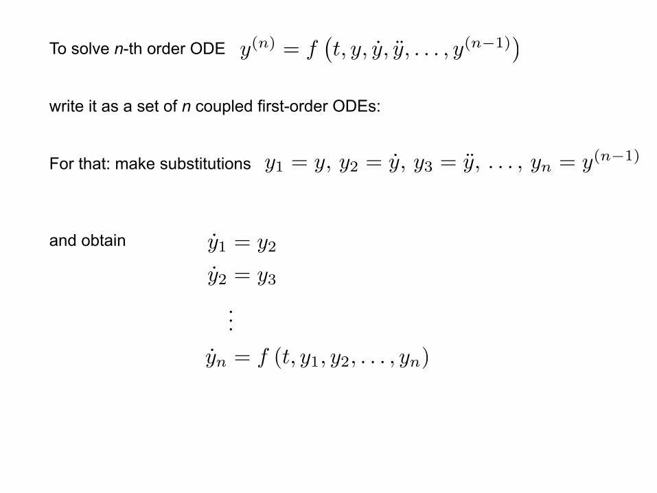
y1 = y2
y2 = y3...
yn = f (t, y1, y2, . . . , yn)
To solve n-th order ODE
write it as a set of n coupled first-order ODEs:
For that: make substitutions
and obtain
y(n) = f�t, y, y, y, . . . , y(n�1)
�
y1 = y, y2 = y, y3 = y, . . . , yn = y(n�1)

y = f(t, y)
y (t0) = y0
Initial value problem: since there are many potential solutions for an ODE, you need to specify initial values:
Example: Solve two coupled ODEs with solver ode45
time interval initial values
In filevdp1.m
Scriptmyscript.m

Plot result:LaTex symbols
Scriptmyscript.m

13. Plotting in 2d & 3dTo plot x versus y (2d plot), use command plot(x,y,’color_style_marker’)
a string, containing between 1 to fourcharacters enclosed by ‘…’, indicatingcolor, line style, and marker type.
Examples:
(1) plot(x,y,’ks’) for black squares at each point and no line (2) plot(x,y,’r:+’) for red-dotted line and plus-sign markers at each data point (3) plot(x,y,’r:+’, ’LineWidth’,2, ’MarkerSize’,10)
same as (2), but thicker line and larger markers

Multiple panels: To arrange plots in Example: four 3d plots a m x n matrix use
draws wireframe meshwith color determined by height Z as a function of Xand Y
plots X versus1:n and 1:m with[m,n]=size(X)
Additional 2d plots are: loglog, semilogx, and semilogy
Other 3d plots are: plot3, contour, and surf

• To download the files log on Blackboard:https://bb.imperial.ac.uk
• The files are also on:http://www.bg.ic.ac.uk/research/g.stan/#Lecture_Notes