Embed Size (px)
Citation preview

Introduction to R/Bioconductor
Introduction to R/Bioconductor
Dr. Pete E. PascuzziAssistant Professor
Purdue University Libraries
July 11, 2016
Introduction to R/Bioconductor
What is R?
R is a computing environment/suite/language for datamanipulation, visualization and analysis (i.e. statistics).R is the ”freeware” version of S and behaves similarly inmany respects.R is comprised of a series of packages that includefunctions and data structures for many disciplines, e.g.bioinformatics, economics, and social sciences.

Introduction to R/Bioconductor
What is R?
R is an interpreted computer language (as opposed to acompiled computer language like C++). The advantage isthat it is easier to program and troubleshoot. Thedisadvantage is that it is slower.R can serve as a ”wrapper”/interface to faster algorithms.R developers include many of the top researchers in theirfields and new statistical methods are often implementedas R code.

Introduction to R/Bioconductor
What is Bioconductor?
Bioconductor is an open source software project thatdevelops tools for the analysis of biological data with R.Bioconductor is a repository for R packages forbioinformatics analyses.Bioconductor is a help resource for bioinformaticians thatuse R.
Introduction to R/Bioconductor
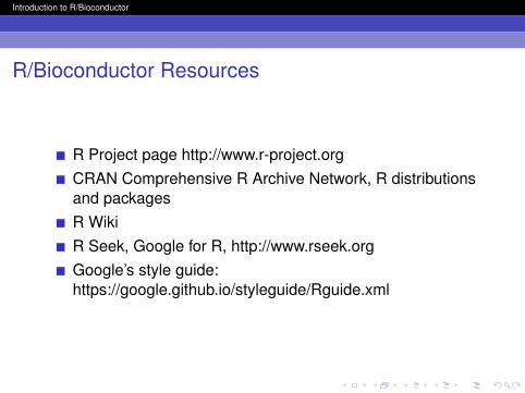
R/Bioconductor Resources
R Project page http://www.r-project.orgCRAN Comprehensive R Archive Network, R distributionsand packagesR WikiR Seek, Google for R, http://www.rseek.orgGoogle’s style guide:https://google.github.io/styleguide/Rguide.xml
Introduction to R/Bioconductor
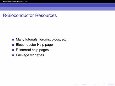
R/Bioconductor Resources
Many tutorials, forums, blogs, etc.Bioconductor Help pageR internal help pagesPackage vignettes

Introduction to R/Bioconductor
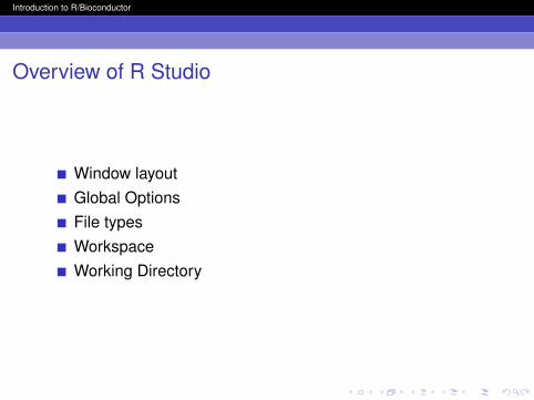
Overview of R Studio
We are going to use R Studio with R because it provides a niceuser interface for R. R Studio is called an IDE (IntegratedDevelopment Environment), a term used by computerprogrammers. R Studio combines an editor, console, history,help, plots, etc. windows in an easy to use layout.
Introduction to R/Bioconductor
Overview of R Studio
Window layoutGlobal OptionsFile typesWorkspaceWorking Directory

Introduction to R/Bioconductor
R’s Steep Learning Curve
Like any computer language, R has a steep learning curve.This is complicated by the fact that anyone can contributepackages for R, and programming style can vary wildly betweenprogrammers. However, the basic syntax of R is pretty simple.
Introduction to R/Bioconductor
Basic R Syntax
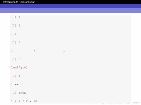
R is an interactive language. If you enter acommand/expression/assignment at the R prompt, R willimmediately evaluate your expression (you don’t need tocompile computer code).
Introduction to R/Bioconductor
1 + 1
[1] 2
1+1
[1] 2
1 + 1
[1] 2
log10(10)
[1] 1
1 == 1
[1] TRUE
1 + 1 / 2 * 10

Introduction to R/Bioconductor
[1] 6
(1 + 1) / 2 * 10
[1] 10
1 + 1 / 2 * 10>= (1 + 1) / 2 * 10
[1] FALSE
"hi"
[1] "hi"
Introduction to R/Bioconductor
Basic R Syntax
Note that in each case, R evaluated your expression andreturned the result to the console. As you can see, R is notgenerally sensitive to spaces in your code because the firstthree expressions all returned 2.

Introduction to R/Bioconductor
Basic R Syntax
In the above examples, we did not save any of our results. Towrite a program that will do anything useful, you must save theresults of your expression to an object. There are manyclasses of object in R from simple integer vectors to specialclasses such as the ExpressionSet which can hold all the datafrom a microarray experiment.You use the Assignment Operator, < −, to create an object.

Introduction to R/Bioconductor
x <- 1 + 1y <- log10(100)x == y #the operator for equality
[1] TRUE
if(x == y) "equal"
[1] "equal"
if(x < y) "less"if(x > y) "greater"
Introduction to R/Bioconductor
Basic R Syntax
So far, we have mostly used operators, a special type offunction that has a simple syntax. You merely string variablesand operators together to form an expression. Functions areoften much more complicated so the programmer must specifycertain arguments (parameters) to the function. In the exampleabove log10 is a function.
Introduction to R/Bioconductor
Basic R Syntax
In the examples above log10 is a function, and the number 10is the only argument. Functions are always followed byparentheses that enclose the arguments. If there are multiplearguments to pass to the function, these arguments must beseparated by commas. Argument/value pairs should beseparated by an equal sign, =. However, the argument nameand equal sign are often omitted for simple functions.

Introduction to R/Bioconductor
y <- log10(x=100)y <- rep(y, 10)x <- seq(from=1, to=10, by=1)plot(x=x, y=y, type="b", main="Simple Plot")

Introduction to R/Bioconductor
2 4 6 8 10
1.5
2.0
2.5Simple Plot
x
y

Introduction to R/Bioconductor
Basic R Syntax
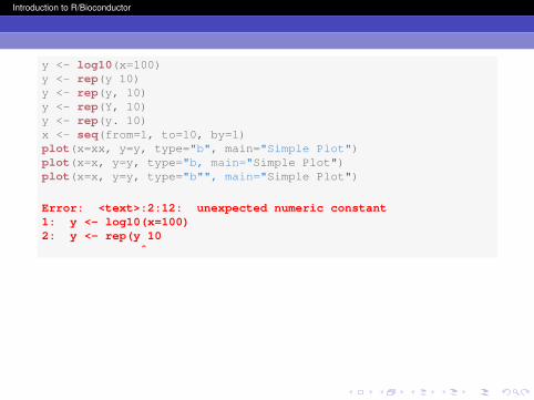
The most common mistakes in R programming are simpletypos. If you make a typo in an object name, then R will not findthat object. Additionally, R is case-sensitive! If you make asyntax mistake (missing commas, inappropriate symbols, etc.),then R will get confused when it tries to evaluate yourexpression.
Introduction to R/Bioconductor
y <- log10(x=100)y <- rep(y 10)y <- rep(y, 10)y <- rep(Y, 10)y <- rep(y. 10)x <- seq(from=1, to=10, by=1)plot(x=xx, y=y, type="b", main="Simple Plot")plot(x=x, y=y, type="b, main="Simple Plot")plot(x=x, y=y, type="b"", main="Simple Plot")
Error: <text>:2:12: unexpected numeric constant1: y <- log10(x=100)2: y <- rep(y 10
ˆ
Introduction to R/Bioconductor
Basic R Syntax
There are also strict and recommended restrictions on variablenames and the use of special characters. Names must beginwith a letter. Numbers are OK later in the name. Avoid specialcharacters other than a period (recommended) or underscorecharacter (not recommended). If you want to emphasize thepresence of words or information in your names, use periods,”camel case” or ”semi camel case”.

Introduction to R/Bioconductor
my.log <- log10(x=100)MyLog <- log10(x=100) #camel casemyLog <- log10(x=100) #semi camel casemy_log <- log10(x=100) #permitted by not recommendedall.equal(my.log, MyLog, myLog, my_log)
[1] TRUE
Introduction to R/Bioconductor
Basic R Syntax
Note that the ”expressions” after the number sign were notevaluated. The number sign is the comment character used toadd comments to your code. Anything on a line after acomment sign will be ignored by R.

Introduction to R/Bioconductor
Getting Help
R has a good built in help system. You can get the details aboutan R function or installed packages from the help menu, e.g.?list.files or help(list.files). Alternatively, if you cannotremember the name of a function, you can do a text search,e.g. ??”partial match” or help.search(”partial match”).

Introduction to R/Bioconductor
Getting Help
Note the help system may not be working on Rice becauseof a compatibility issue between R 3.2.3 and R Studio onLinux systems. We will try launching the help system inFirefox.

Introduction to R/Bioconductor
help.start()
starting httpd help server ...done
If the browser launched by '/usr/bin/open' is already running, itis *not* restarted, and you must switch to its window.
Otherwise, be patient ...
Introduction to R/Bioconductor
R Vignettes
A vignette is a PDF document that accompanies an Rpackage. A good vignette will provide essential information onthe intended use of a package. You can get a list of thevignettes for your installed packages with this expression,vignette(). A list of vignettes should appear in the upper leftwindow of R Studio. To open a specific vignette, provide thevignette name as well.

Introduction to R/Bioconductor
Computer Terminology
To learn R, you need to understand how information is storedand organized on your computer, and how R works in thecontext of this organization.
Directory - A ”place” where files are located, i.e. a folder.Path - A series of directories that lead to the location of afile and possibly terminating with a file name.File - Self-contained information in a myriad of formatsavailable to your operating system (OS) or other programs.Try to use open rather than proprietary formats as much aspossible.Object - R stores information (possibly from reading files)in memory as objects. Do not confuse objects and files!

Introduction to R/Bioconductor
Working Directory
R has a default directory when you open a session. This shouldbe your home directory on your computer and may looksomething like this: C:/Users/yourname/Documents or/Users/YourName/Documents. Unless you specify a path, Rwill always look for files in, and send output, to the currentorworking directory. Your first step when you start an Rsession should be to carefully choose, or create, andappropriate working directory.
Introduction to R/Bioconductor
Working Environment
R stores data as objects in memory. This environment is calledyour workspace or working environment. Students oftenconfuse files in their working directory with objects in theirworking environment.
Introduction to R/Bioconductor
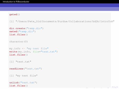
getwd()
[1] "/Users/Pete_Old/Documents/Purdue/Collaborations/bd2k/IntroToR"
dir.create("temp.dir")setwd("temp.dir")list.files()
character(0)
my.info <- "my test file"write(my.info, file="test.txt")list.files()
[1] "test.txt"
readLines("test.txt")
[1] "my test file"
unlink("test.txt")list.files()

Introduction to R/Bioconductor
character(0)
setwd("..")list.files()
[1] "figure" "IntroToR.nav" "IntroToR.pdf"[4] "IntroToR.R" "IntroToR.Rnw" "IntroToR.snm"[7] "IntroToR.tex" "IntroToR.toc" "Session01_2016.Rnw"
[10] "Session02_2016.Rnw" "temp.dir" "workspace.RData"
unlink("temp.dir")list.files()
[1] "figure" "IntroToR.nav" "IntroToR.pdf"[4] "IntroToR.R" "IntroToR.Rnw" "IntroToR.snm"[7] "IntroToR.tex" "IntroToR.toc" "Session01_2016.Rnw"
[10] "Session02_2016.Rnw" "temp.dir" "workspace.RData"
unlink("temp.dir", recursive=TRUE)list.files()
[1] "figure" "IntroToR.nav" "IntroToR.pdf"[4] "IntroToR.R" "IntroToR.Rnw" "IntroToR.snm"[7] "IntroToR.tex" "IntroToR.toc" "Session01_2016.Rnw"
[10] "Session02_2016.Rnw" "workspace.RData"

Introduction to R/Bioconductor
Basic R Syntax
This example illustrates an important part of R syntax.Character vectors are always enclosed by quotes (double orsingle). There were two cases above, the character vector ”mytest file” and the name of the file, ”text.txt”. Function and objectnames are never enclosed by quotes.
Introduction to R/Bioconductor
Working Environment
In addition to your working directory, R stores data as objectsin memory. This environment is called your workspace orworking environment. Don’t confuse the two. Students oftenconfuse files in their working directory with objects in theirtextbfworking environment.

Introduction to R/Bioconductor
Working Environment
When you quit R, it will ask if you want to save your workspace(all the objects in your working environment). If you enter yes,R will write a binary file to your working directory with thename ”.RData”. On most operating systems, this is a hiddenfile–you won’t see it when you browse the folders on yourcomputer. This is a problem because, depending on yourproject, ”.RData” can be very large. Better to use save.imageand choose a good file name.

Introduction to R/Bioconductor
ls()
[1] "my_log" "my.info" "my.log" "myLog" "MyLog" "x" "y"
rm(my_log, my.info)ls()
[1] "my.log" "myLog" "MyLog" "x" "y"
save.image()list.files()
[1] "figure" "IntroToR.nav" "IntroToR.pdf"[4] "IntroToR.R" "IntroToR.Rnw" "IntroToR.snm"[7] "IntroToR.tex" "IntroToR.toc" "Session01_2016.Rnw"[10] "Session02_2016.Rnw" "workspace.RData"
list.files(all=TRUE)
[1] "." ".." ".DS_Store"[4] ".RData" "figure" "IntroToR.nav"[7] "IntroToR.pdf" "IntroToR.R" "IntroToR.Rnw"[10] "IntroToR.snm" "IntroToR.tex" "IntroToR.toc"[13] "Session01_2016.Rnw" "Session02_2016.Rnw" "workspace.RData"

Introduction to R/Bioconductor
unlink(".RData")list.files(all=TRUE)
[1] "." ".." ".DS_Store"[4] "figure" "IntroToR.nav" "IntroToR.pdf"[7] "IntroToR.R" "IntroToR.Rnw" "IntroToR.snm"
[10] "IntroToR.tex" "IntroToR.toc" "Session01_2016.Rnw"[13] "Session02_2016.Rnw" "workspace.RData"
save.image("workspace.RData")list.files()
[1] "figure" "IntroToR.nav" "IntroToR.pdf"[4] "IntroToR.R" "IntroToR.Rnw" "IntroToR.snm"[7] "IntroToR.tex" "IntroToR.toc" "Session01_2016.Rnw"[10] "Session02_2016.Rnw" "workspace.RData"

Introduction to R/Bioconductor
Objects
R is an object-oriented programming language. This meansthat functions take an objects as arguments and produce anobject as a result. (Confusingly, functions are also consideredR objects.) Objects are a specialized data structures used tostore information. Some objects can be very simple (a numericconstant), while others are very complex (a completemicroarray experiment).
Introduction to R/Bioconductor
Objects
Objects have properties such as mode, class, and type thatdetermine what type of information that they can store and howfunctions will act upon them. In many cases, objects will alsohave attributes such as names, row names, or column names.You can get more information about an object with str() whichwill display the structure of the object.
Introduction to R/Bioconductor
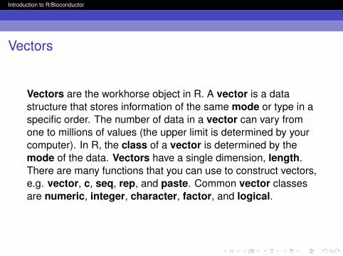
Vectors
Vectors are the workhorse object in R. A vector is a datastructure that stores information of the same mode or type in aspecific order. The number of data in a vector can vary fromone to millions of values (the upper limit is determined by yourcomputer). In R, the class of a vector is determined by themode of the data. Vectors have a single dimension, length.There are many functions that you can use to construct vectors,e.g. vector, c, seq, rep, and paste. Common vector classesare numeric, integer, character, factor, and logical.
Introduction to R/Bioconductor
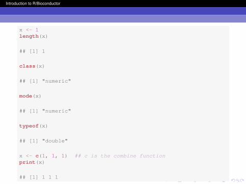
x <- 1length(x)
## [1] 1
class(x)
## [1] "numeric"
mode(x)
## [1] "numeric"
typeof(x)
## [1] "double"
x <- c(1, 1, 1) ## c is the combine functionprint(x)
## [1] 1 1 1

Introduction to R/Bioconductor
length(x)
## [1] 3
class(x)
## [1] "numeric"
mode(x)
## [1] "numeric"
typeof(x)
## [1] "double"
x <- c("one, one, one")print(x)
## [1] "one, one, one"
length(x) ## does this surprise you?

Introduction to R/Bioconductor
## [1] 1
class(x)
## [1] "character"
mode(x)
## [1] "character"
typeof(x)
## [1] "character"
x <- c("one", "one", "one")print(x)
## [1] "one" "one" "one"
length(x)
## [1] 3

Introduction to R/Bioconductor
class(x)
## [1] "character"
mode(x)
## [1] "character"
typeof(x)
## [1] "character"
x <- rep("one", 3)print(x)
## [1] "one" "one" "one"
x <- seq(from = 1, to = 10, by = 1)length(x)
## [1] 10

Introduction to R/Bioconductor
print(x)
## [1] 1 2 3 4 5 6 7 8 9 10
y <- x == 2mode(y)
## [1] "logical"
print(y)
## [1] FALSE TRUE FALSE FALSE FALSE FALSE FALSE FALSE FALSE FALSE
## create an 'empty' vector initialized to 0x <- vector(mode = "integer", length = 10)print(x)
## [1] 0 0 0 0 0 0 0 0 0 0
x <- 1:10print(x)
## [1] 1 2 3 4 5 6 7 8 9 10

Introduction to R/Bioconductor
x <- vector(mode = "character", length = 10)print(x)
## [1] "" "" "" "" "" "" "" "" "" ""
x <- factor(c(rep("red", 5), rep("white", 2), rep("blue", 3)), levels = c("red","white", "blue"))
table(x)
## x## red white blue## 5 2 3

Introduction to R/Bioconductor
Vector Names and Indexing
You can select data value(s) from a vector by indexing. You cando this with the names assigned to the vector (not the objectname itself) or with the position in the vector. To extract valuesfrom a vector you must the Extract operators, the squarebrackets [].

Introduction to R/Bioconductor
tom.wins <- 1:4 ## another way to construct a vectornames(tom.wins) <- paste("day", 1:4, sep = "_")print(tom.wins)
## day_1 day_2 day_3 day_4## 1 2 3 4
attributes(tom.wins)
## $names## [1] "day_1" "day_2" "day_3" "day_4"
tom.wins[1]
## day_1## 1
tom.wins[-1]
## day_2 day_3 day_4## 2 3 4
tom.wins["day_1"]

Introduction to R/Bioconductor
## day_1## 1
tom.wins[c(2, 4)]
## day_2 day_4## 2 4
good.days <- tom.wins[tom.wins >= 3]print(good.days)
## day_3 day_4## 3 4
## indexing vectorsmy.index <- tom.wins >= 3tom.wins[my.index]
## day_3 day_4## 3 4
my.index <- which(tom.wins >= 3)tom.wins[my.index]
Introduction to R/Bioconductor
## day_3 day_4## 3 4
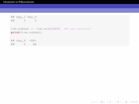
tom.subset <- tom.wins[4:5] ## use caution!print(tom.subset)
## day_4 <NA>## 4 NA

Introduction to R/Bioconductor
Vectorization of Functions and the Recycling Rule
Many functions in R are designed to act on vectors in a singleoperation. One of the keys to developing fast R code is tounderstand this powerful feature. However, you must usecaution when performing operations on vectors of unequallength because R will usually recycle the values from theshorter vector to complete the operations on the longer vector.Remember this recycling rule when you write your code!

Introduction to R/Bioconductor
temp.dat <- 1:10more.dat <- 1:2print(temp.dat + 1) ## 1 is recycled
## [1] 2 3 4 5 6 7 8 9 10 11
print(temp.dat + more.dat) ## 1 and 2 are recylced.
## [1] 2 4 4 6 6 8 8 10 10 12

Introduction to R/Bioconductor
Arrays
Arrays are similar to vectors, but they can have manydimensions. A matrix is the special case of a 2 x 2 array (like atable). Vectors, arrays and matrices are all alike in that they cancontain data only of the same mode or type. Like vectors, theelements in an array can be named and indexed. In R,dimension 1 is rows and 2 is columns. Beyond that, you shouldsimply think of the dimensions as ”slices” of the larger datastructure.
Introduction to R/Bioconductor
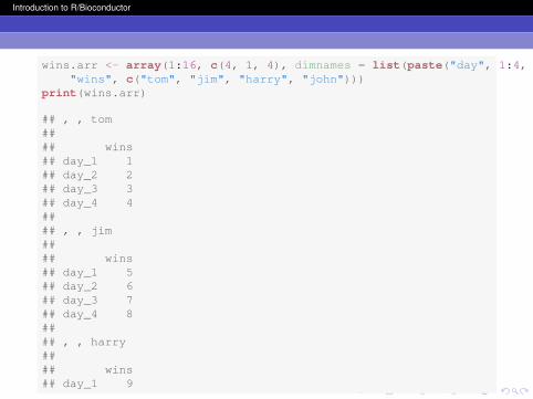
wins.arr <- array(1:16, c(4, 1, 4), dimnames = list(paste("day", 1:4, sep = "_"),"wins", c("tom", "jim", "harry", "john")))
print(wins.arr)
## , , tom#### wins## day_1 1## day_2 2## day_3 3## day_4 4#### , , jim#### wins## day_1 5## day_2 6## day_3 7## day_4 8#### , , harry#### wins## day_1 9

Introduction to R/Bioconductor
## day_2 10## day_3 11## day_4 12#### , , john#### wins## day_1 13## day_2 14## day_3 15## day_4 16
length(wins.arr) ## I find this surprising
## [1] 16
str(wins.arr)
## int [1:4, 1, 1:4] 1 2 3 4 5 6 7 8 9 10 ...## - attr(*, "dimnames")=List of 3## ..$ : chr [1:4] "day_1" "day_2" "day_3" "day_4"## ..$ : chr "wins"## ..$ : chr [1:4] "tom" "jim" "harry" "john"
Introduction to R/Bioconductor
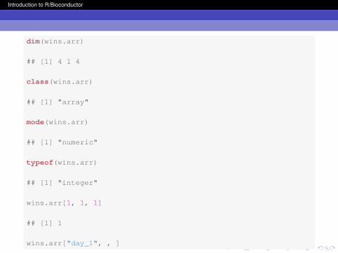
dim(wins.arr)
## [1] 4 1 4
class(wins.arr)
## [1] "array"
mode(wins.arr)
## [1] "numeric"
typeof(wins.arr)
## [1] "integer"
wins.arr[1, 1, 1]
## [1] 1
wins.arr["day_1", , ]

Introduction to R/Bioconductor
## tom jim harry john## 1 5 9 13
wins.arr[, , "harry"]
## day_1 day_2 day_3 day_4## 9 10 11 12

Introduction to R/Bioconductor
Matrices
A matrix is the special case of a 2 x 2 array, and a verycommon class of object. By default, a matrix is constructed bycolumn rather than row, although this can be changed. Thereare three common functions that create a matrix, matrix(),cbind(), and rbind().

Introduction to R/Bioconductor
wins.mat <- matrix(1:16, nrow = 4, ncol = 4)rownames(wins.mat) <- paste("day", 1:4, sep = "_")colnames(wins.mat) <- c("tom", "jim", "harry", "john")print(wins.mat)
## tom jim harry john## day_1 1 5 9 13## day_2 2 6 10 14## day_3 3 7 11 15## day_4 4 8 12 16
length(wins.mat)
## [1] 16
dim(wins.mat)
## [1] 4 4
class(wins.mat)
## [1] "matrix"

Introduction to R/Bioconductor
mode(wins.mat)
## [1] "numeric"
typeof(wins.mat)
## [1] "integer"
## add another column with averagesaverages <- apply(wins.mat, 1, mean)wins.mat <- cbind(wins.mat, averages)wins.mat
## tom jim harry john averages## day_1 1 5 9 13 7## day_2 2 6 10 14 8## day_3 3 7 11 15 9## day_4 4 8 12 16 10
Introduction to R/Bioconductor
Data frames
Data frames are similar to matrices except each column of adata frame can contain data of a different mode. In many ways,data frames are analogous to Excel spreadsheets, althoughdata frames do not contain formulas to calculate values basedon other cells (although you can perform a similar assignmentin R).
Introduction to R/Bioconductor
Data frames
Data frames are rectangular, the rows of a data frame alwayshave the same number of columns and vice-versa. A dataframe is a special case of a list. You can add new columns orrows to your data frame at any time with a simple assingment.You will probably find yourself using dataframes frequently forbioinformatics.
Introduction to R/Bioconductor
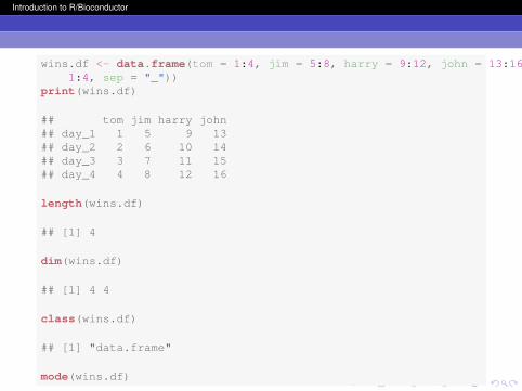
wins.df <- data.frame(tom = 1:4, jim = 5:8, harry = 9:12, john = 13:16, row.names = paste("day",1:4, sep = "_"))
print(wins.df)
## tom jim harry john## day_1 1 5 9 13## day_2 2 6 10 14## day_3 3 7 11 15## day_4 4 8 12 16
length(wins.df)
## [1] 4
dim(wins.df)
## [1] 4 4
class(wins.df)
## [1] "data.frame"
mode(wins.df)

Introduction to R/Bioconductor
## [1] "list"
typeof(wins.df)
## [1] "list"
## add another column with averageswins.df$avr <- apply(wins.df, 1, mean)wins.df["day_5", ] <- c(1, 1, 1, 1, 1)print(wins.df)
## tom jim harry john avr## day_1 1 5 9 13 7## day_2 2 6 10 14 8## day_3 3 7 11 15 9## day_4 4 8 12 16 10## day_5 1 1 1 1 1

Introduction to R/Bioconductor
Data Frame Names and Indexing
The naming and indexing of data frames is slightly differentthan vectors. Data frames have row names and column names.These can be assigned when you create the data frame orassigned or renamed with rownames or colnames. You canalso select elements, row, or columns in a data frame withmatrix-style indices. An individual column of a data frame canbe selected with the dollar sign.

Introduction to R/Bioconductor
colnames(wins.df)
## [1] "tom" "jim" "harry" "john" "avr"
rownames(wins.df)
## [1] "day_1" "day_2" "day_3" "day_4" "day_5"
print(wins.df$tom)
## [1] 1 2 3 4 1
print(wins.df["day_1", ])
## tom jim harry john avr## day_1 1 5 9 13 7
print(wins.df["day_4", "harry"])
## [1] 12

Introduction to R/Bioconductor
Lists
Lists are a mode of vector where each element in the list canhave a different mode and even different length. This can beparticularly useful if you want to group related informationtogether for subsequent analysis. Like data frames, you canadd additional elements to a list. Many R functions return a listso get accustomed to using them.

Introduction to R/Bioconductor
wins.list <- list(tom = 1:4, jim = 5:8, harry = 9:12, john = 13:16)names(wins.list$tom) <- names(wins.list$jim) <- names(wins.list$harry) <- names(wins.list$john) <- paste("day",
1:4, sep = "_")print(wins.list)
## $tom## day_1 day_2 day_3 day_4## 1 2 3 4#### $jim## day_1 day_2 day_3 day_4## 5 6 7 8#### $harry## day_1 day_2 day_3 day_4## 9 10 11 12#### $john## day_1 day_2 day_3 day_4## 13 14 15 16
length(wins.list)
## [1] 4
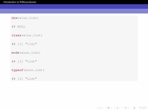
Introduction to R/Bioconductor
dim(wins.list)
## NULL
class(wins.list)
## [1] "list"
mode(wins.list)
## [1] "list"
typeof(wins.list)
## [1] "list"

Introduction to R/Bioconductor
Indexing Lists
Each element in the list can have a name and each value inthat element can also have a name. Indexing of list can be byelement name similar to column name for data frames, and bythe data value in that element. For lists, single square brackets,double square brackets and dollar signs can be used.

Introduction to R/Bioconductor
wins.list$tom
## day_1 day_2 day_3 day_4## 1 2 3 4
wins.list[["tom"]]
## day_1 day_2 day_3 day_4## 1 2 3 4
wins.list[c("tom", "harry")]
## $tom## day_1 day_2 day_3 day_4## 1 2 3 4#### $harry## day_1 day_2 day_3 day_4## 9 10 11 12
wins.list[["john"]][2:3]
## day_2 day_3## 14 15

Introduction to R/Bioconductor
When to Use Each Class of Data Structure?
There is no simple answer to that question, but basically youuse the data structure that best suits the data and yourintended analyses. In many cases, a data frame will be the bestanswer, but, for example, you might need to use a function thatonly acts on a matrix. In this case, there are rapid ways toswitch between formats.
Introduction to R/Bioconductor
Finding and Installing Packages
R comes with a number of base packages that are sufficient formany purposes. However, you can expand R’s capabilities witha huge number of additional packages. For example,Bioconductor is a ”suite” of packages designed forbioinformatics. We have installed all packages that are requiredfor this course.
Introduction to R/Bioconductor
Comprehensive R Archive Network (CRAN)
CRAN and, it’s many mirrors, is the place to go to install R andmany R packages, i.e. add-ons. Most of our packages will beinstalled from Bioconductor, but CRAN is still an importantresource.

Introduction to R/Bioconductor
Comprehensive R Archive Network (CRAN)
Go to CRAN
http://cran.r-project.org
You can find, download, and install R foryour computer.

Introduction to R/Bioconductor
Bioconductor
Bioconductor has over 2400 packages for bioinformatics. Thisincludes software for data visualization analysis, annotationdata and experimental data.

Introduction to R/Bioconductor
Bioconductor
Go to Bioconductor
https://www.bioconductor.org
You can find, download, and installbioinformatics packages.

Introduction to R/Bioconductor
Session Information
options(width=40)sessionInfo();
## R version 3.2.2 (2015-08-14)## Platform: x86_64-apple-darwin13.4.0 (64-bit)## Running under: OS X 10.10.5 (Yosemite)#### locale:## [1] en_US.UTF-8/en_US.UTF-8/en_US.UTF-8/C/en_US.UTF-8/en_US.UTF-8#### attached base packages:## [1] stats graphics grDevices## [4] utils datasets methods## [7] base##

Introduction to R/Bioconductor
## other attached packages:## [1] knitr_1.13#### loaded via a namespace (and not attached):## [1] magrittr_1.5 formatR_1.4## [3] tools_3.2.2 stringi_1.1.1## [5] highr_0.6 stringr_1.0.0## [7] evaluate_0.9