Introduction to R

Phil SpectorStatistical Computing Facility

Department of StatisticsUniversity of California, Berkeley

1

Some Basics

• There are three types of data in R: numeric, character and

logical.

• R supports vectors, matrices, lists and data frames.

• Objects can be assigned values using an equal sign (=) or the

special <- operator.

• R is highly vectorized - almost all operations work equally well

on scalars and arrays

• All the elements of a matrix or vector must be of the same type

• Lists provide a very general way to hold a collection of

arbitrary R objects.

• A data frame is a cross between a matrix and a list – columns

(variables) of a data frame can be of different types, but they

all must be the same length.

2

Using R

• Typing the name of any object will display a printed

representation. Alternatively, the print() function can be

used to display the entire object.

– Element numbers are displayed in square brackets

– Typing a function’s name will display its argument list and

definition, but sometimes it’s not very enlightening.

• The str() function shows the structure of an object

• If you don’t assign an expression to an R object, R will display

the results, but they are also stored in the .Last.value object

• Function calls require parentheses, even if there are no

arguments. For example, type q() to quit R.

• Square brackets ([ ]) are used for subscripting, and can be

applied to any subscriptable value.

3

Getting Data into R

• c() - allows direct entry of small vectors in programs.

• scan() - reads data from a file, a URL, or the keyboard into a

vector.

– Can be embedded in a call to matrix() or array().

– Use the what= argument to read character data.

• read.table - reads from a file or URL into a dataframe.

– sep= allows a field separator other than white space.– header= specifies if the first line of the file contains variable

names.– as.is= allows control over character to factor conversion– Specialized versions of read.table() include read.csv()

(comma-separated values), read.delim() (tab-separated

values), and read.fwf (fixed width formatted data).

• data() - reads preloaded data sets into the current

environment.

4

Where R stores your data

Each time you start R, it looks for a file called .RData in the

current directory. If it doesn’t exist it creates it. So managing

multiple projects is easy - change to a different directory for each

different project.

When you end an R session, you will be asked whether or not you

want to save the data.

• You can use the objects() function to list what objects exist

in your local database, and the rm() function to remove ones

you don’t want.

• You can start R with the --save or --no-save option to avoid

being prompted each time you exit R.

• You can use the save.image() function to save your data

whenever you want

5

Getting Help

To view the manual page for any R function, use the

help(functionname ) command, which can be abbreviated by

following a question mark (?) by the function name.

The help.search("topic ") command will often help you get

started if you don’t know the name of a function.

The command help.start() will open a browser pointing to a

variety of (locally stored) information about R, including a search

engine and access to more lengthly PDF documents. Once the

browser is open, all help requests will be displayed in the browser.

Many functions have examples, available through the example()

function; general demonstrations of R capabilities can be seen

through the demo() function.

6

Libraries

Libraries in R provide routines for a large variety of data

manipulation and analysis. If something seems to be missing from

R, it is most likely available in a library.

You can see the libraries installed on your system with the

command library() with no arguments. You can view a brief

description of the library using library(help=libraryname )

Finally, you can load a library with the command

library(libraryname )

Many libraries are available through the CRAN (Comprehensize R

Archive Network) at

http://cran.r-project.org/src/contrib/PACKAGES.html .

You can install libraries from CRAN with the install.packages()

function, or through a menu item in Windows. Use the lib.loc=

argument if you don’t have administrative permissions.

7

Search Path

When you type a name into the R interpreter, it checks through

several directories, known as the search path, to determine what

object to use. You can view the search path with the command

search(). To find the names of all the objects in a directory on

the search path, type objects(pos=num ), where num is the

numerical position of the directory on the search path.

You can add a database to the search path with the attach()

function. To make objects from a previous session of R available,

pass attach() the location of the appropriate .RData file. To refer

to the elements of a data frame or list without having to retype the

object name, pass the data frame or list to attach(). (You can

temporarily avoid having to retype the object name by using the

with() function.)

8

Sizes of Objects

The nchar() function returns the number of characters in a

character string. When applied to numeric data, it returns the

number of characters in the printed representation of the number.

The length() function returns the number of elements in its

argument. Note that, for a matrix, length() will return the total

number of elements in the matrix, while for a data frame it will

return the number of columns in the data frame.

For arrays, the dim() function returns a list with the dimensions of

its arguments. For a matrix, it returns a vector of length two with

the number of rows and number of columns. For convenience, the

nrow() and ncol() functions can be used to get either dimension

of a matrix directly. For non-arrays dim() returns a NULL value.

9

Finding Objects

The objects() function, called with no arguments, prints the

objects in your working database. This is where the objects you

create will be stored.

The pos= argument allows you look in other elements of your

search path. The pat= argument allows you to restrict the search

to objects whose name matches a pattern. Setting the all.names=

argument to TRUE will display object names which begin with a

period, which would otherwise be suppressed.

The apropos() function accepts a regular expression, and returns

the names of objects anywhere in your search path which match

the expression.

10

get() and assign()

Sometimes you need to retreive an object from a specific database,

temporarily overiding R’s search path. The get() function accepts

a character string naming an object to be retreived, and a pos=

argument, specifying either a position on the search path or the

name of the search path element. Suppose I have an object named

x in a database stored in rproject/.RData . I can attach the

database and get the object as follows:

> attach("rproject/.RData")

> search()

[1] ".GlobalEnv" "file:rproject/.RData" "package:methods"

[4] "package:stats" "package:graphics" "package:grDevices"

[7] "package:utils" "package:datasets" "Autoloads"

[10] "package:base"

> get("x",2)

The assign() function similarly lets you store an object in a

non-default location.

11

Combining Objects

The c() function attempts to combine objects in the most general

way. For example, if we combine a matrix and a vector, the result

is a vector.

> c(matrix(1:4,ncol=2),1:3)

[1] 1 2 3 4 1 2 3

Note that the list() function preserves the identity of each of its

elements:

> list(matrix(1:4,ncol=2),1:3)

[[1]]

[,1] [,2]

[1,] 1 3

[2,] 2 4

[[2]]

[1] 1 2 3

12

Combining Objects (cont’d)When the c() function is applied to lists, it will return a list:> c(list(matrix(1:4,ncol=2),1:3),list(1:5))

[[1]]

[,1] [,2]

[1,] 1 3

[2,] 2 4

[[2]]

[1] 1 2 3

[[3]]

[1] 1 2 3 4 5

To break down anything into its individual components, use the

recursive=TRUE argument of c():

> c(list(matrix(1:4,ncol=2),1:3),recursive=TRUE)

[1] 1 2 3 4 1 2 3

The unlist() and unclass() functions may also be useful.

13

Subscripting

Subscripting in R provides one of the most effective ways to

manipulate and select data from vectors, matrices, data frames and

lists. R supports several types of subscripts:

• Empty subscripts - allow modification of an object while

preserving its size and type.x = 1 creates a new scalar, x, with a value of 1, while

x[] = 1 changes each value of x to 1.

Empty subscripts also allow refering to the i-th column of a

data frame or matrix as matrix[i,] or the j -th row as

matrix[,j].

• Positive numeric subscripts - work like most computer

languagesThe sequence operator (:) can be used to refer to contigious

portions of an object on both the right- and left- hand side of

assignments; arrays can be used to refer to non-contigious

portions.

14

Subscripts (cont’d)• Negative numeric subscripts - allow exclusion of selected

elements

• Zero subscripts - subscripts with a value of zero are ignored• Character subscripts - used as an alternative to numeric

subscripts

Elements of R objects can be named. Use names() for vectors

or lists, dimnames(), rownames() or colnames() for data

frames and matrices. For lists and data frames, the notation

object$name can also be used.

• Logical subscripts - powerful tool for subsetting and modifying

data

A vector of logical subscripts, with the same dimensions as

the object being subscripted, will operate on those elements

for which the subscript is TRUE.

Note: A matrix indexed with a single subscript is treated as a

vector made by stacking the columns of the matrix.

15

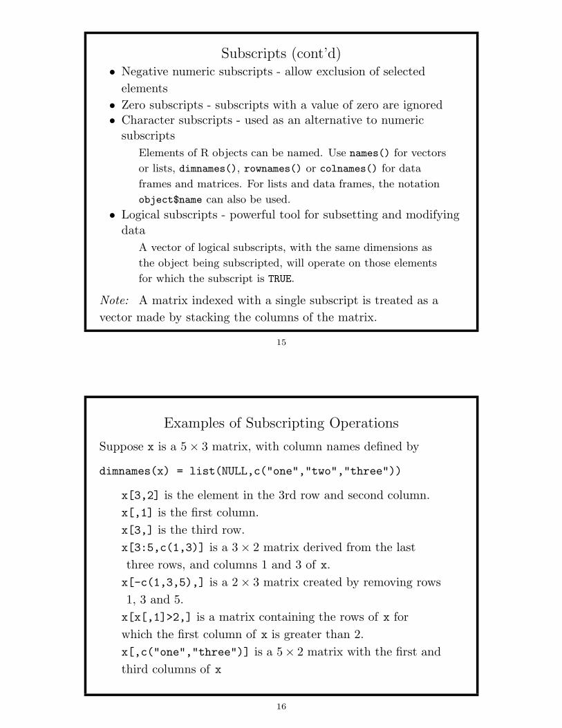
Examples of Subscripting Operations

Suppose x is a 5 × 3 matrix, with column names defined by

dimnames(x) = list(NULL,c("one","two","three"))

x[3,2] is the element in the 3rd row and second column.

x[,1] is the first column.

x[3,] is the third row.

x[3:5,c(1,3)] is a 3 × 2 matrix derived from the last

three rows, and columns 1 and 3 of x.

x[-c(1,3,5),] is a 2 × 3 matrix created by removing rows

1, 3 and 5.

x[x[,1]>2,] is a matrix containing the rows of x for

which the first column of x is greater than 2.

x[,c("one","three")] is a 5× 2 matrix with the first and

third columns of x

16

More on Subscripts

By default, when you extract a single column from a matrix or

data.frame, it becomes a simple vector, which may confuse some

functions. Furthermore, if the column was named, the name will be

lost. To prevent this from happening, you can pass the drop=TRUE

argument to the subscript operator:

> mx = matrix(c(1:4,4:7,5:8),ncol=3,byrow=TRUE,

+ dimnames=list(NULL,c("one","two","three")))

> mx[,3]

[1] 3 5 5 8

> mx[,3,drop=FALSE]

three

[1,] 3

[2,] 5

[3,] 5

[4,] 8

17

[[ Subscripting Operator

A general principle in R is that subscripted objects retain the mode

of their parent. For vectors and arrays, this rarely causes a

problem, but for lists (and data frames treated like lists), R will

often have problems working directly with such objects.

> mylist = list(1:10,10:20,30:40)

> mean(mylist[1])

[1] NA

Warning message:

argument is not numeric or logical: returning NA in: mean.default(mylist[1])

For this purpose, R provides double brackets for subscripts, which

extract the actual list element, not a list containing the element:

> mean(mylist[[1]])

[1] 5.5

For named lists, the problem can also be avoided using the $

notation.

18

Subscripting with Data Frames

Since a data frame is a cross between a matrix and a list,

subscripting operations for data frames are slightly different than

for either of those types.

• Double subscripts in a data frame behave exactly as with matrices.

• Single subscripts in a data frame refer to a data frame containing

the appropriate columns. To extract the actual column(s), use

double brackets or an empty first subscript.

• A dollar sign ($) can be used to separate a data frame name from a

column name to extract the actual column. If the column name has

special characters, it must be surrounded by quotes.

x[["name"]], x[,"name"] and x$name are all equivalent, but

x["name"] is a data frame with one column.

x[1,"name"], x[1,]$name or x[1,]["name"] all access name for

the first observation.

19

Tables and Matrices

If a two column matrix is used as a subscript of a matrix, its rows

are interpreted as row and column numbers, for both accessing and

assigning values.

> a = matrix(c(1,1,1,2,2,3),ncol=2,byrow=TRUE)

> a

[,1] [,2]

[1,] 1 1

[2,] 1 2

[3,] 2 3

> x = matrix(0,nrow=4,ncol=3)

> x[a] = c(10,20,30)

> x

[,1] [,2] [,3]

[1,] 10 20 0

[2,] 0 0 30

[3,] 0 0 0

[4,] 0 0 0

20

Type Conversion Functions

Occasionally it is necessary to treat an object as if it were of a

different type. One of the most common cases is to treat a

character value as if it were a number. The as.numeric() function

takes care of this, and in general there are “as.” functions for most

types of objects encountered in R. A complete list can be seen with

apropos(’^as.’); some common examples are as.matrix(),

as.integer(), as.data.frame(), as.list(), as.logical(), and

as.vector().

These functions do not permanently change the type of their

arguments.

Some functions related to type conversion include round() and

trunc() for numeric values, and paste() for character values.

21

Some Functions for Vectors

• c() - combines values, vectors, and/or lists to create new

objects.

• unique() - returns a vector containing one element for each

unique value in the vector

• duplicated() - returns a logical vector which tells if elements

of a vector are duplicated with regard to previous ones.

• rev() - reverse the order of elements in a vector

• sort() - sorts the elements in a vector.

• append() - append or insert elements in a vector.

• sum() - sum of the elements of a vector

• min() - minimum value in a vector

• max() - maximum value in a vector

22

Missing Values

In R, missing values are represented by the string NA. You can

assign a missing value by setting a variable equal to NA, but you

must use the is.na() function to test for a missing value.

Missing values are propagated in all calculations, so the presence of

even a single missing value can result in a variety of problems.

Many statistical functions provide a na.rm= argument to remove

missing values before computations. Alternatively, use logical

subscripting to easily extract non-missing values:

> values = c(12,NA,19,15,12,17,14,NA,19)

> values[!is.na(values)]

[1] 12 19 15 12 17 14 19

> vv = matrix(values,ncol=3,byrow=TRUE)

> vv[!is.na(vv[,2]),,drop=FALSE]

[,1] [,2] [,3]

[1,] 15 12 17

23

Reading R’s Input from a File

The source() command accepts a file name or a URL, and

executes the commands from the file or URL, just as if they were

typed into the R interpreter.

If an error is encountered while source is processing a file,

execution halts, and the remaining statements are not evaluated.

R’s usual default of printing unassigned expressions is suppressed

in source(), unless the echo=TRUE argument is used.

Note that scan() can read data into an R object, but the contents

of the files accessed by source() are executed as R commands in

the current R session. You can combine both capabilities by

embedding a scan command inside of a file whose name will be

passed to source.

24

Alternative Input: Connections

In addition to filenames, scan() and read.table() will accept a

variety of connection functions, allowing data to be read from

pipes, zipped files, URLs and sockets. (“help(connections)”

provides complete information.) For example, the output of the

UNIX ps command looks like this:

PID TTY TIME CMD

26377 pts/1 00:00:00 tcsh

26392 pts/1 00:00:02 R

26647 pts/1 00:00:00 ps

The following commands read the output of the ps command into a

data frame:

> read.table(pipe("ps"),header=TRUE)

PID TTY TIME CMD

1 26377 pts/1 00:00:00 tcsh

2 26392 pts/1 00:00:02 R

3 26647 pts/1 00:00:00 ps

25

PrintingThe print() function can be used to print any R object, and is

silently invoked when an expression is not assigned to a value. For

lists and arrays, it will always include subscripting information.> print(7)

[1] 7

> print(matrix(c(1,2,3,4),ncol=2))

[,1] [,2]

[1,] 1 3

[2,] 2 4

The cat() function allows you to print the values of objects

without any subscripting information. It accepts a variable number

of (unnamed) input arguments and supports the following named

arguments:• file= filename or connection object to write to

• sep= character string to insert between objects

• fill= logical or numeric value determining automatic newlines

• append= should output be appended if file= was used

26

Output Destinations

By default, the output from an interactive R session is sent to the

screen. To divert this output to a file, use the sink() or

capture.output() function. These provide an exact copy of the

session’s output.

To write the contents of a matrix or vector to a file, use the

write() function. Remember that when writing a matrix, it will

be written to the file by columns, so the transpose function (t())

may be useful. The ncolumns= argument can be used to specify the

number of data values on each line; the append= argument can be

used to avoid overwriting an existing file.

To write a data frame to a file, use the write.table() function; it

is basically the mirror image of the read.table() function.

27

Recycling of VectorsWhen a vector is involved in an operation that requires more

elements than the vector contains, the values in the vector are

recycled.

> x = matrix(1:3,nrow=2,ncol=6)

> x

[,1] [,2] [,3] [,4] [,5] [,6]

[1,] 1 3 2 1 3 2

[2,] 2 1 3 2 1 3

A warning is printed if the desired length is not an even multiple of

the original vector’s length.> matrix(1:4,nrow=2,ncol=5)

[,1] [,2] [,3] [,4] [,5]

[1,] 1 3 1 3 1

[2,] 2 4 2 4 2

Warning message:

data length [4] is not a sub-multiple or multiple of the number of

columns [5] in matrix

28

OperatorsAll of the binary operators in R are vectorized, operating element

by element on their arguments, recycling values as needed. These

operators include:

+ addition - subtraction * multiplication

/ division ^ Exponentiation %% Modulus

%/% Integer Division

Comparison operators will return the logical values TRUE or FALSE,

or NA if any elements involved in a comparison are missing.

< less than > greater than <= l.t. or equal

>= g.t. or equal == equality != non-equality

Logical operators come in elementwise and pairwise forms.

& elementwise and && pairwise and ! negation

| elementwise or || pairwise or xor() exclusive or

The %in% operator can be used to test if a value is present in a

vector or array.

29

Rounding Functions

The following functions are available for rounding numerical values:

• round() - uses IEEE standard to round up or down; optional

digits= argument controls precision

• signif() - rounds numerical values to the specified digits=

number of significant digits

• trunc() - rounds by removing non-integer part of number

• floor(), ceiling() - rounds to integers not greater or not

less than their arguments, respectively

• zapsmall() - accepts a vector or array, and makes numbers

close to zero (compared to others in the input) zero. digits=

argument controls the rounding.

30

Non-vectorized functions

Although most functions in R are vectorized, returning objects which are

the same size and shape as their input, some will always return a single

logical value.

any() tests if any of the elements of its arguments meet a particular

condition; all() tests if they all do.

> x = c(7,3,12,NA,13,8)

> any(is.na(x))

[1] TRUE

> all(x > 0)

[1] NA

> all(x > 0,na.rm=TRUE)

[1] TRUE

identical() tests if two objects are exactly the same. all.equal()

allows for a tolerance= argument when dealing with numeric values, but

returns a character string summarizing differences. You can test for

numeric equality using a tolerance by combining the two:

> x = c(3.0001,4.0009,5.002)

> y = c(3,4,5)

> identical(all.equal(x,y,tolerance=.001),TRUE)

[1] TRUE

31

Using Logical Expressions

We’ve seen that logical expressions can be effectively used to

extract or modify subsets of data within vectors and arrays. Some

other ways to use logical expressions include:

• Counting

The sum() function will automatically coerse FALSE to 0

and TRUE to 1, so taking the sum of a logical expression

counts how many elements are TRUE.

• Locations

The which() function will return the positions within an

array or vector for which a logical expression is TRUE. By

default it treats arrays as column-wise vectors; the

arr.ind=TRUE argument can be used to return array

indices instead.

32

Categorical Variables

Categorical variables in R are known as factors, and are stored as

integer codes along with a set of labels. The cut() function creates

factors from continuous variables.

> x = c(17,19,22,43,14,8,12,19,20,51,8,12,27,31,44)

> cut(x,3)

[1] (7.96,22.3] (7.96,22.3] (7.96,22.3] (36.7,51] (7.96,22.3] (7.96,22.3]

[7] (7.96,22.3] (7.96,22.3] (7.96,22.3] (36.7,51] (7.96,22.3] (7.96,22.3]

[13] (22.3,36.7] (22.3,36.7] (36.7,51]

Levels: (7.96,22.3] (22.3,36.7] (36.7,51]

> cut(x,3,labels=c("low","medium","high"))

[1] low low low high low low low low low high

[11] low low medium medium high

Levels: low medium high

To return the codes in an ordinary (non-factor) variable, use the

labels=FALSE argument.

To convert a factor to its integer codes, use the unclass() function; to

convert to ordinary character values use as.character().

33

Categorical Variables (cont’d)

You can control where cut() divides up your data using the

breaks= argument. Given an integer, cut() breaks up the data at

equal intervals; using a vector of values breaks up the data at those

values. For example, to create quartiles, the breaks can be specified

as the output from the quantile() function:

> cut(x,breaks=quantile(x,c(0,.25,.50,.75,1)),

+ labels=c("Q1","Q2","Q3","Q4"),include.lowest=TRUE)

[1] Q2 Q2 Q3 Q4 Q2 Q1 Q1 Q2 Q3 Q4 Q1 Q1 Q3 Q4 Q4

Levels: Q1 Q2 Q3 Q4

Note the use of include.lowest=TRUE to insure that the minimum

value is not set to missing.

34

The rep() function

The rep() function generates repetitions of values. The first

argument to rep() is a vector containing the values to be repeated.

If the second argument is a scalar, the entire first argument is

repeated that many times; if it’s a vector of the same length as the

first argument, each element of the first list is repeated as many

times as the corresponding element in the second list.

> rep(1:3,3)

[1] 1 2 3 1 2 3 1 2 3

> rep(1:3,c(5,2,1))

[1] 1 1 1 1 1 2 2 3

For the special case of generating levels for designed experiments,

the gl() function provides a convenient wrapper.

35

Tabulation

The table() function is the main tool for tabulating data in R.

Given a vector, it produces a frequency table:

> x = c(7,12,19,7,19,21,12,14,17,12,19,21)

> table(x)

x

7 12 14 17 19 21

2 3 1 1 3 2

Notice that the output is named based on the data values. To use

them as numbers, they must be passed to the as.numeric()

function:

> sum(table(x) * as.numeric(names(table(x))))

[1] 180

36

Cross-tabulation

If several equal length vectors are passed to table(), it will output

an array with the counts of the vector’s cross-tabulation:

> x1 = c(1,2,3,2,1,3,2,3,1)

> x2 = c(2,1,2,3,1,3,2,2,3)

> x3 = c(1,2,3,3,2,1,2,1,2)

> table(x1,x2)

x2

x1 1 2 3

1 1 1 1

2 1 1 1

3 0 2 1

For higher-dimensioned tables (producing higher-dimensioned

arrays), the default output may not be very easy to use. The

ftable() function can be used to ”flatten” such a table.

37

ftable()

> tbl = table(x1,x2,x3)

> tbl

, , x3 = 1

x2

x1 1 2 3

1 0 1 0

2 0 0 0

3 0 1 1

, , x3 = 2

x2

x1 1 2 3

1 1 0 1

2 1 1 0

3 0 0 0

, , x3 = 3

x2

x1 1 2 3

1 0 0 0

2 0 0 1

3 0 1 0

> ftable(tbl)

x3 1 2 3

x1 x2

1 1 0 1 0

2 1 0 0

3 0 1 0

2 1 0 1 0

2 0 1 0

3 0 0 1

3 1 0 0 0

2 1 0 1

3 1 0 0

38

Date Values

The as.Date() function converts a variety of character date

formats into R dates, stored as the number of days since January 1,

1970. The format= argument is a string composed of codes such as

%Y for full year, %y for 2-digit year, %m for month number, and %d

for day number.

Once converted to dates, the following functions will return

information about dates: weekdays(), months(), quarters() and

julian().

In addition, the cut() function allows the following choices for the

breaks= argument: "day", "week", "month", or "year".

Note: Alternative date and time formats are available through the

chron and POSIXct libraries.

39

Date Values: Examples

The format= argument allows a variety of formats:

> d1 = as.Date("20041201",format="%Y%m%d")

> d2 = as.Date("12/5/03",format="%m/%d/%y")

> d3 = as.Date("7-8-2001",format="%d-%m-%Y")

Many operators and functions will recognize dates.

> d1 - d2

Time difference of 362 days

> d1 - d2 > 360

[1] TRUE

> mean(c(d1,d2,d3))

[1] "2003-06-25"

> d1 > d2

[1] TRUE

40

The chron library

The chron library provides an alternative representation for date

values. In addition to dates, chron objects can also store times.

The chron() function accepts separate arguments for dates= and

times=. Similary, the format= argument can be a vector or list

with named dates and/or times elements. Formats for dates can

be composed of m, d, y, month, day, or year; times can be

composed of h, m, and s.

If the date=argument to chron() is numeric, it is interpreted as a

Julian date; the origin= argument accepts a array of length 3

specifying a month, day and year for an alternative to the default

January 1, 1970 origin.

The functions as.Date() and as.chron() can be used to convert

between the two representations of dates.

41

chron library: Examples

When using chron’s default formats (m/d/y and h:m:s), the

formats= argument is not needed.

> d1 = chron(’12/25/2004’,’0:0:0’) # default formats

The origin= argument is useful with Julian dates:

> d2 = chron(10,origin=c(12,31,2004))

> d2

[1] 01/10/05

Operations and functions which work with Date objects will usually work with

chron objects:

> d3 = chron(’7-6-2005’,’6:00:00’,format=c(dates=’m-d-y’,times=’h:m:s’))

> d3 - d1

Time in days:

[1] 193.25

> weekdays(d3)

[1] Wed

Levels: Sun < Mon < Tue < Wed < Thu < Fri < Sat

42

File System Interface

R provides a variety of functions to query and manipulate the file

system.

• file.info() - accepts a character vector of filenames, and

returns a data frame with information about the files.

• file.access() - provides information about read, write and

execute access of files

• list.files() - returns a list of files from a given directory

• file.choose() - interactive file chooser, varies by operating

system

The following functions are also available:

file.create() file.exists() file.remove()

file.rename() file.append() file.copy()

file.symlink() dir.create() file.show()

43

Operating System Interface

In addition to pipes, R provides the following functions to access

and execute operating system commands

• system - executes an operating system command; with

intern=TRUE returns the command’s output, otherwise the

system return code.

• system.time() - accepts and executes an R expression, and

returns the execution time

• proc.time() - returns user, system and total time for the

current R process and its children

• Sys.info() - information about the operating system

• Sys.time() - returns the current time from the operating

system

44

Assignment Functions

Many functions in R can be used on the left hand side of an

assignment operator, allowing various properties of objects to be

modified conveniently. Some examples include names(), diag(),

dimnames(), length(), dim() and substr().

For example, one way to reshape a matrix would be to assign a

value to the dim() function:

> m = matrix(1:12,4,3)

> m

[,1] [,2] [,3]

[1,] 1 5 9

[2,] 2 6 10

[3,] 3 7 11

[4,] 4 8 12

> dim(m) <- c(6,2)

> m

[,1] [,2]

[1,] 1 7

[2,] 2 8

[3,] 3 9

[4,] 4 10

[5,] 5 11

[6,] 6 12

Functions such as these have names which end in “<-”.

45

Writing Functions: Introduction

• Function definitions begin with the word function, followed by

a parenthetic list of arguments.

• Writing functions in R is easy because the syntax is identical to

ordinary R syntax.

• Variables which are modified in a function are local to the

function, but all variables in the calling environment are

available (read only). (You can override this using the <<-

operator.)

• You can specify a return value through the return() function;

otherwise, a function’s return value is the value of the last

evaluated expression. (Use the invisible() function to

suppress the return value from being automatically displayed)

46

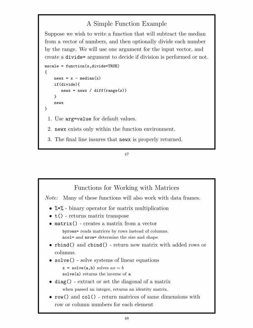
A Simple Function Example

Suppose we wish to write a function that will subtract the median

from a vector of numbers, and then optionally divide each number

by the range. We will use one argument for the input vector, and

create a divide= argument to decide if division is performed or not.

mscale = function(x,divide=TRUE)

{

newx = x - median(x)

if(divide){

newx = newx / diff(range(x))

}

newx

}

1. Use arg=value for default values.

2. newx exists only within the function environment.

3. The final line insures that newx is properly returned.

47

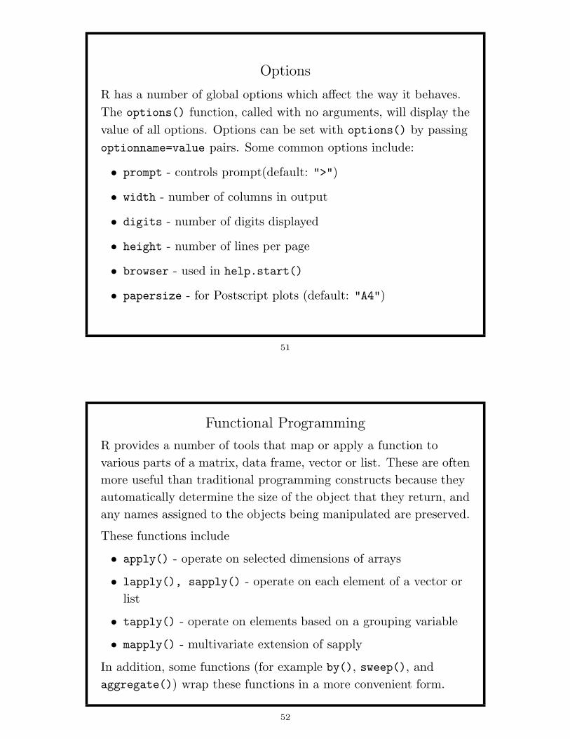
Functions for Working with Matrices

Note: Many of these functions will also work with data frames.

• %*% - binary operator for matrix multiplication

• t() - returns matrix transpose

• matrix() - creates a matrix from a vector

byrows= reads matrices by rows instead of columns.

ncol= and nrow= determine the size and shape

• rbind() and cbind() - return new matrix with added rows or

columns.

• solve() - solve systems of linear equations

x = solve(a,b) solves ax = b

solve(a) returns the inverse of a

• diag() - extract or set the diagonal of a matrix

when passed an integer, returns an identity matrix.

• row() and col() - return matrices of same dimensions with

row or column numbers for each element

48

Generating Sequences

The colon (:) operator creates simple integer sequences. While it is

often used as a subscript to “slice” an array, it can also be used on

its own

> letters[10:15]

[1] "j" "k" "l" "m" "n" "o"

> x = 1:100

> mean(x)

[1] 50.5

The seq() function provides more control over the generated

sequence. The first two arguments to seq() give the starting and

ending values. Additional arguments include by= to specify an

increment other than 1, or, alternatively length= to specify the

number of elements in the generated sequence.

To generate a sequence for use in looping over an object, the

along= argument can be used.

49

sample()

The sample() function returns random samples or permutations of

a vector. Passed an integer, n, it returns a random permutation of

the integers from 1 to n.

The size= argument specifies the size of the returned vector.

The prob= argument provides a vector of probabilities for sampling.

By default, sampling is done without replacement; the

replace=TRUE option will result in a random sample from the

specified input.

> sample(10)

[1] 7 6 1 2 8 9 3 4 10 5

> sample(c("a","b","c","d","e"),size=10,replace=TRUE)

[1] "d" "c" "b" "b" "c" "a" "a" "e" "b" "a"

> sample(c("a","b","c"),size=10,prob=c(.5,.25,.25),replace=TRUE)

[1] "c" "b" "a" "a" "a" "a" "a" "c" "c" "a"

50

Options

R has a number of global options which affect the way it behaves.

The options() function, called with no arguments, will display the

value of all options. Options can be set with options() by passing

optionname=value pairs. Some common options include:

• prompt - controls prompt(default: ">")

• width - number of columns in output

• digits - number of digits displayed

• height - number of lines per page

• browser - used in help.start()

• papersize - for Postscript plots (default: "A4")

51

Functional Programming

R provides a number of tools that map or apply a function to

various parts of a matrix, data frame, vector or list. These are often

more useful than traditional programming constructs because they

automatically determine the size of the object that they return, and

any names assigned to the objects being manipulated are preserved.

These functions include

• apply() - operate on selected dimensions of arrays

• lapply(), sapply() - operate on each element of a vector or

list

• tapply() - operate on elements based on a grouping variable

• mapply() - multivariate extension of sapply

In addition, some functions (for example by(), sweep(), and

aggregate()) wrap these functions in a more convenient form.

52

apply()

apply() will execute a function on every row or every column of a

matrix. Suppose the data frame finance contains the variables

Name, Price, Volume and Cap, and we want the mean of each of the

numerical variables.

> apply(finance[-1],2,mean)

Price Volume Cap

21.46800 51584.51840 NA

The ”2” passed as the second argument to apply means ”columns”.

Note that the variable names were retained.

If additional arguments need to be passed to the function, they can

simply be passed to apply:

> apply(finance[-1],2,mean,na.rm=TRUE)

Price Volume Cap

21.46800 51584.51840 123.22597

53

lapply() and sapply()

These functions apply a function to each element of a list or vector.

lapply() always returns a list; sapply() will return a vector or

array if appropriate.

One important use of these functions is to correctly process the

columns of a data frame. Since apply() is designed for matrices, it

can’t retain the mode of individual data frame columns. Thus,

commands like the following don’t work:

> apply(finance,2,is.numeric)

names Price Volume Cap

FALSE FALSE FALSE FALSE

Using sapply() solves the problem:

> sapply(finance,is.numeric)

names Price Volume Cap

FALSE TRUE TRUE TRUE

54

tapply()

tapply() allows you to map a function to a vector, broken up into

groups defined by a second vector or list of vectors. Generally the

vectors will all be from the same matrix or data frame, but they

need not be.

Suppose we have a data frame called banks with columns name,

state and interest.rate, and we wish to find the maximum

interest rate for banks in each of the states.

with(banks,tapply(interest.rate,state,max,na.rm=TRUE))

Note the use of the with() function to avoid retyping the data

frame name (banks) when refering to its columns.

55

The by() function

tapply() is simple to use when the variable being analyzed is a

vector, but it becomes difficult to use when we wish to perform an

analysis involving more than one variable. For example, suppose we

have a data frame named df with four variables: group, x, y, and

z, and we wish to calculate the correlation matrix of the last three

variables for each level of group. To use tapply we would have to

manipulate the indices of the data frame, but the by() function

takes care of this automatically. The statement

by(df,df$group,cor)

returns a list with as many correlation matrices as there were levels

of the variable group.

56

aggregate()

The aggregate() function presents a summary of a scalar valued

statistic, broken down by one or more groups. While similar

operations can be performed using tapply(), aggregate()

presents the results in a data frame instead of a table.

> testdata = data.frame(one=c(1,1,1,2,2,2),two=c(1,2,3,1,2,3),

+ three=rnorm(6))

> aggregate(testdata$three,list(testdata$one,testdata$two),mean)

Group.1 Group.2 x

1 1 1 -0.62116475

2 2 1 -0.68367887

3 1 2 0.53058202

4 2 2 -0.61788020

5 1 3 0.02823623

6 2 3 -1.01561697

> tapply(testdata$three,list(testdata$one,testdata$two),mean)

1 2 3

1 -0.6211648 0.5305820 0.02823623

2 -0.6836789 -0.6178802 -1.01561697 \

57

aggregate() (cont’d)

If the first argument to aggregate() is a matrix or multicolumn

data frame, the statistic will be calculated separately for each

column.

> testdata = cbind(sample(1:5,size=100,replace=TRUE),

+ matrix(rnorm(500),100,5))

> dimnames(testdata) = list(NULL,c("grp","A","B","C","D","E"))

> aggregate(testdata[,-1],list(grp=testdata[,1]),min)

grp A B C D E

1 1 -2.362126 -2.777772 -1.8970320 -2.152187 -1.966436

2 2 -1.690446 -2.202395 -1.6244721 -1.637200 -1.036338

3 3 -2.078137 -1.571017 -2.0555413 -1.401563 -1.881126

4 4 -1.325673 -1.660392 -0.8933617 -2.205563 -1.749313

5 5 -1.644125 -1.518352 -2.4064893 -1.664716 -1.994624

Note that the data frame returned by aggregate() has the

appropriate column names, and that grouping variable names can

be supplied with the list of grouping variables.

58

split()

While by() and aggregate() simplify many tasks which arise in

data manipulation, R provides the split() function which takes a

data frame, and creates a list of data frames by breaking up the

original data frame based on the value of a vector. In addition to

being useful in its own right, the returned list can be passed to

lapply() or sapply() as an alternative way of doing repetitive

analyses on subsets of data.

> data(Orange)

> trees = split(Orange,Orange$Tree)

> sapply(trees,function(x)coef(lm(circumference~age,data=x)))

3 1 5 2 4

(Intercept) 19.20353638 24.43784664 8.7583446 19.9609034 14.6376202

age 0.08111158 0.08147716 0.1110289 0.1250618 0.1351722

A similar result could be achieved by using

> by(Orange,Orange$Tree,function(x)coef(lm(circumference~age,data=x)))

59

The if/else statement

Like most programming languages, R provides an if/else construct.

The basic form is

if (condition) expression

else other_expression

where the else clause is optional. Note that the condition must be a

scalar; if not, only the first value of the condition is used. In all cases,

expressions must be surrounded by curly braces if they consists of more

than one line, and the

R also provides the ifelse() function, which takes three arguments: an

object containing logical values, the value to return for true elements,

and the value to return for false elements. It returns an object the same

size as its first argument.

> z = c(7,10,-3,4,12,-5)

> ifelse(z>0,z,0)

[1] 7 10 0 4 12 0

60

Loops in R

R provides three types of loops, although they are not used as often

as most other programming languages.

• for loop

for(var in sequence) expression

• while loop

while(condition) expression

• repeat loop

repeat expression

In all cases, the expressions must be surrounded by curly braces if

they are more than one line long.

Unassigned objects are not automatically printed inside of loops –

you must explicitly use the print() or cat() functions.

To terminate loops at any time, use the break statement; to

continue to the next iteration use the next statement.

61

Sorting

The sort() function will return a sorted version of a vector.

> x = c(19,25,31,15,12,43,82,22)

> sort(x)

[1] 12 15 19 22 25 31 43 82

The function order() returns a permutation vector which will

reorder a vector so that it becomes sorted. This is especially useful

if you wish to sort a matrix by the values in one of it’s rows:

> mat = matrix(c(12,3,7,9,10,11),ncol=2)

> mat

[,1] [,2]

[1,] 12 9

[2,] 3 10

[3,] 7 11

> mat[order(mat[,1]),]

[,1] [,2]

[1,] 3 10

[2,] 7 11

[3,] 12 9

62

Character Strings: paste()

The paste() function converts its arguments into character strings,

and concatenates them. To specify a separator between the strings,

use the sep= argument. Like most R functions, paste is vectorized:

> paste("x",1:5,sep="")

[1] "x1" "x2" "x3" "x4" "x5"

To create a result that is a single string, use the collapse=

argument.

> paste("x",1:5,collapse="|",sep="*")

[1] "x*1|x*2|x*3|x*4|x*5"

One use of paste is to convert numeric values to character values:

> x = c("10"=110,"7"=107,"12"=112)

> x[paste(3 + 7)]

10

110

63

Character Strings: substring()The substring() function extracts substrings from character

strings. The first= and last= arguments specify the size of the

desired substring. Like most R functions, it is vectorized:> animals = c("dog","cat","chicken","goat","sheep")

> substring(animals,2,4)

[1] "og" "at" "hic" "oat" "hee"

By default, the last= argument is set to a large number, so if you

omit last=, substring() simply extracts until the end of the

string.

An assignment form of substring() is also available, although it

will not allow the resulting string to shrink or grow:

> pet = "Rover"

> substring(pet,2,3) = ’abcd’

> pet

[1] "Raber"

Note that only 2 characters were replaced in pet.

64

Splitting Character Strings

Many times a character string consists of several “words” which

need to be separated. The strsplit() function accepts a character

string and a regular expressions to split the character string, and

returns a vector with the split pieces of the string. If the regular

expression is of length 0, the string is split into individual

characters.

The function is fully vectorized, and when the first argument is a

vector of character strings, strsplit() will always return a list.

> strs = c("the razor toothed piranhas","of the genera Serrasalmus")

> strsplit(strs,c(" ",""))

[[1]]

[1] "the" "razor" "toothed" "piranhas"

[[2]]

[1] "o" "f" " " "t" "h" "e" " " "g" "e" "n" "e" "r" "a" " " "S" "e" "r" "r" "a"

[20] "s" "a" "l" "m" "u" "s"

65

Character Strings: Searching for Patterns

The grep() function searches for regular expressions in vectors of

character strings. The first argument to grep() is the pattern to

be searched for, and the second argument is the vector of strings to

be searched. grep returns the indices of those elements in the

vector which matched the pattern; with the value=TRUE argument,

it returns the actual matches.

To find the locations of the patterns within the strings, the

regexpr() function can be used with the same two required

arguments as grep. It returns a vector of positions where the

pattern was found, or -1 if the pattern was not found; in addition

the returned value has an attribute containing the length of the

match.

The argument perl=TRUE can be passed to either function to use

perl-style regular expressions.

66

Searching for Patterns (cont’d)

The following simple example shows the returned values from

grep() and regexpr(). The regular expression a[lm] means an

”a” followed by either an ”l” or an ”m”.

> states = c("Alabama","Alaska","California","michigan")

> grep("a[lm]",states,ignore.case=TRUE)

[1] 1 2 3

> regexpr("a[lm]",states)

[1] 5 -1 2 -1

attr(,"match.length")

[1] 2 -1 2 -1

You can retrieve attributes of stored objects with the attr()

function.

67

Text Substitution

The functions sub() and gsub() can be used to create new

character strings by replacing regular expressions (first argument)

with replacement strings (second argument) in an existing

string(third argument). The ignore.case=TRUE argument can be

provided to ignore the case of the regular expression.

The only difference between the two functions is that sub() will

only replace the first occurence of a regular expression within

elements of its third argument, while gsub replaces all such

occurences.

> vars = c("date98","size98","x98weight98")

> sub(’98’,’04’,vars)

[1] "date04" "size04" "x04weight98"

> gsub(’98’,’04’,vars)

[1] "date04" "size04" "x04weight04"

68

match() and pmatch()

The match() function accepts two vector arguments, and returns a

vector of the same length as the first argument, containing the

indices in the second argument that matched elements of the first

argument. The nomatch= argument, which defaults to NA, specifies

what is returned when no match occurs.

> match(1:10,c(7,2,5,4,3),nomatch=0)

[1] 0 2 5 4 3 0 1 0 0 0

For character values, pmatch() allows for partial matching,

meaning that extra characters at the end are ignored when

comparing strings of different length.

To get a logical vector instead of positions, use the %in% operator.

69

Merging Matrices and Dataframes

Many times two matrices or data frames need to be combined by

matching values in a column in one to values in a column of the

other. Consider the following two data frames:

> one

a b

1 1 12

2 7 18

3 9 24

4 3 19

> two

a y

1 9 108

2 3 209

3 2 107

4 7 114

5 8 103

We wish to combine observations with common values of a in the

two data frames. The merge() function makes this simple:

> merge(one,two,by="a")

a b y

1 3 19 209

2 7 18 114

3 9 24 108

70

Merging Matrices and Dataframes (cont’d)By default, only the rows that matched are included in the output.

Using the all=TRUE argument will display all the rows, adding NAs

where appropriate.

> merge(one,two,by="a",all=TRUE)

a b y

1 1 12 NA

2 2 NA 107

3 3 19 209

4 7 18 114

5 8 NA 103

6 9 24 108

To prevent sorting of the by= variable, use sort=FALSE.

A vector of names or column numbers can be given for the by=

argument to perform a merge on multiple columns.

If the matrices to be merged need to be treated differently, the

arguments by.x=, by.y=, all.x= and all.y= can be used.

71

reshape()

Suppose we have a data frame named firmdata, with several

observations of a variable x recorded at each of several times, for

each of several firms, and we wish to create one observation per

firm, with new variables for each of the values of x contained in

that observation. In R terminology, the original format is called

”long”, and the desired format is called ”wide”.

Our original data set would look like this:

firm time x

7 1 7

7 2 19

7 3 12

12 1 13

12 2 18

12 3 9

19 1 21

19 2 15

19 3 7

72

reshape(), cont’d

The following arguments to reshape explain the role that the

variables play in the transformation. Each argument is a character

string or vector of strings.

• timevar= the variable which specifies which new variable will

be created from a given observation

• idvar= the variable which identifies the unique observations in

the new data set. There will be one observation for each level

of this variable.

• v.names= the variables of interest which were recorded multiple

times

• direction= "long" or "wide" to described the desired result

• varying= when converting to ”long” format, the variables

which will be broken up to create the new (v.names) variable.

73

reshape(), cont’d

The following R statements perform the desired transformation:

> newdata = reshape(firmdata,timevar="time",idvar="firm",

+ v.names="x",direction="wide")

> newdata

firm x.1 x.2 x.3

1 7 7 19 12

4 12 13 18 9

7 19 21 15 7

Once converted, a call to reshape() in the opposite direction needs

no other arguments, because the reshaping information is stored

with the data.

74

expand.grid()

The expand.grid() function accepts vectors or lists of vectors, and

creates a data frame with one row for each combination of values

from the vectors. Combined with apply(), it can easily perform a

grid search over a specified range of values.

> values = expand.grid(x=seq(-3,3,length=10),

y=seq(-3,3,length=10))

> result = cbind(values,

result=apply(values,1,function(z)sin(z[1])*cos(z[2])))

> dim(result)

[1] 100 3

> result[which(result[,3] == max(result[,3])),]

x y result

3 -1.666667 -3 0.9854464

93 -1.666667 3 0.9854464

75

Probability Distributions and Random Numbers

R provides four types of functions for dealing with distributions.

Each type begins with a letter designating its purpose, followed by

a name specifying the distribution.

• q - quantile function (argument is probability - returns deviate)

• p - probability (argument is deviate, returns probability)

• d - density (argument is deviate, returns density value)

• r - random numbers (argument is n, returns vector of random

numbers)

Among the possible distributions are:

norm Normal exp Exponential gamma Gamma

pois Poisson binom Binomial chisq Chi-square

t Student’s t f F unif Uniform

76

Descriptive Statistics

Among the functions for descriptive, univariate statistics are

mean() median() range() kurtosis()∗ skewness()∗

var() mad() sd() IQR() weighted.mean()∗ - in e1071 library

All of these functions accept an argument na.rm=TRUE to ignore missing

values.

The stem() function produces a (ASCII) stem-and-leaf diagram; the

boxplot() function produces a high-quality representation.

The cor() function computes correlations among multiple variables.

(Specify cases to use with the use= argument, with choices "all.obs"

(default), "complete.obs", or "pairwise.complete.obs". )

The summary() function provides minimum, mean, maximum and

quartiles in a single call.

The quantile() function returns the values of any desired quantiles

(percentiles).

77

Hypothesis Tests

R provides a number of functions for simple hypothesis testing.

They each have a alternative= argument (with choices

two.sided, less, and greater), and a conf.level= argument for

prespecifying a confidence level.

Among the available functions are:

prop.test Equality of proportions wilcox.test Wilcoxon test

binom.test One sample binomial chisq.test Contingency tables

t.test Student’s t-test var.test Equality of variances

cor.test Correlation coefficient ks.test Goodness of fit

For example, the following code performs a t-test on two unequal

sized groups of data:

> x = c(12,10,19,22,14,22,19,14,15,18,12)

> y = c(18,13,12,13,21,14,12,10,11,9)

> t.test(x,y,alt="two.sided",conf.level=.95)

78

Results of t.test()

Welch Two Sample t-test

data: x and y

t = 1.6422, df = 18.99, p-value = 0.117

alternative hypothesis: true difference in means

is not equal to 0

95 percent confidence interval:

-0.766232 6.348050

sample estimates:

mean of x mean of y

16.09091 13.30000

79

Statistical Models in R

R provides a number of functions for statistical modeling, along

with a variety of functions that extract and display information

about those models. Using object-oriented design principles, most

modeling functions work in similar ways and use similar arguments,

so changing a modeling strategy is usually very simple. Among the

modeling functions available are:

lm() Linear Models aov Analysis of Variance

glm Generalized Linear Models gam1 Generalized Additive Models

tree Classification and Regression Trees cph2 Cox Proportional Hazards

nls Non-linear Models loess Local Regression Models

Some of the functions which display information about models are

summary(), coef(), predict(), resid() and plot().

1 - in mgcv library 2 - in Design library

80

Formulas

R provides a notation to express the idea of a statistical model

which is used in all the modeling functions, as well as some

graphical functions. The dependent variable is listed on the

left-hand side of a tilde (~), and the independent variables are

listed on the right-hand side, joined by plus signs (+).

Most often, the variables in a formula come from a data frame, but

this is not a requirement; in addition expressions involving

variables can also be used in formulas

Inside of formulas, some symbols have special meanings, as shown

below.

+ add terms - remove terms : interaction

* crossing %in% nesting ^ limit crossing

To protect an arithmetic expression inside of a formula, use the I()

function.

81

Example of Formulas

Additive Model

y ~ x1 + x2 + x3

Additive Model without Intercept

y ~ x1 + x2 + x3 - 1

Regress response versus all other variables in data frame

response ~ .

Fully Factorial ANOVA model (a, b, and c are factors)

y ~ a*b*c

Factorial ANOVA model limited to depth=2 interactions

y ~ (a*b*c)^2

Polynomial Regression

y ~ x + I(x^2) + I(x^3)

82

Common Arguments to Modeling Functions

The following arguments are available in all of the modeling

functions:

• formula= first argument – specifies the model

• data= specify a data frame to attach for the duration of the

model

• subset= logical expression to select data to be used

• weights= vector of weights to be applied to model

• na.action= function to preprocess data regarding missing

values

– na.fail prints error message

– na.omit default, omit observations with missing values

– na.pass do nothing

83

Graphics in R

The graphics system in R consists of three components:

• High level functions - These functions produce entire plots with

a single command. Examples include barplot(), boxplot(),

contour(), dotchart(), hist(), pairs(), persp(), pie(),

and plot().

• Low level functions - These functions add to existing plots.

Examples include abline(), arrows(), axis(), frame(),

legend(), lines(), points(), rug(), symbols(), text(), and

title()

• Graphics parameters - Accessed through either plotting

commands or the par() function, these are arguments that

change the layout or appearance of a plot. These parameters

control thing like margins, text size, tick marks, plotting style,

and overall size of the plot.

84

Device Drivers

. By default, a window will automatically be opened to display

your graphics. Some other devices available include postscript(),

pdf(), bitmap() and jpeg(). (See the help for Devices for a

complete list.)

To use an alternative driver, either call the appropriate function

before plotting, or use the dev.copy() function to specify a device

to which to copy the current plot, always ending with a call to

dev.off().

For example, to create a PostScript plot, use statements like

postscript(file="myplot.ps")

... plotting commands go here ...

dev.off()

To create a jpeg image from the currently displayed plot, use

dev.copy(device=jpeg,file="picture.jpg")

dev.off()

85

Multiple Plots on a Page

The graphics parameters mfrow=c(nrow,ncol ) or

mfcol=c(nrow,ncol ) allow multiple plots of equal size to be placed

on a page in an nrow×ncol array. When using mfrow=, plots are

drawn by rows and with mfcol= they are drawn by column.

Since these parameters determine the layout of subsequent plots

they can only be specified through the par() function, and they

must be set before any plotting commands are entered.

Suppose we wish to create a 2 × 2 array of plots of various

trigonometric functions, plotted in the range of −π to π. The

following code uses the curve() function to produce the plots:

par(mfrow=c(2,2))

curve(sin(x),from=-pi,to=pi,main="Sine")

curve(cos(x),from=-pi,to=pi,main="Cosine")

curve(tan(x),from=-pi,to=pi,main="Tangent")

curve(sin(x)^2/cos(x),from=-pi,to=pi,main="Sin^2/Cosine")

86

Multiple Plots on a Page

−3 −2 −1 0 1 2 3

−1.

0−

0.5

0.0

0.5

1.0

Sine

x

sin(

x)−3 −2 −1 0 1 2 3

−1.

0−

0.5

0.0

0.5

1.0

Cosine

x

cos(

x)

−3 −2 −1 0 1 2 3

0.0e

+00

1.0e

+16

Tangent

x

tan(

x)

−3 −2 −1 0 1 2 3

0.0e

+00

5.0e

+15

1.0e

+16

1.5e

+16

Sin^2/Cosine

x

sin(

x)^2

/cos

(x)

The margins can be reduced through the graphics parameters mar=

or mai= for the inner margins, and oma= or omi= for the outer

margins.

87

Plot Types

The plot() function accepts a type= argument, which can be set

to any of the following values: "p" for points, "l" for lines, "b" for

both, "s" for stairstep, and "n" for none.

By setting type="n", axes will be drawn, but no points will be

displayed, allowing multiple lines to be plotted on the same set of

axes. (The matplot() function is also useful in this setting.)

> data(USArrests)

> popgroup = cut(USArrests$UrbanPop,3,labels=c("Low","Medium","High"))

> plot(range(USArrests$Murder),range(USArrests$Rape),type="n",

+ xlab="Murder",ylab="Rape")

> points(USArrests$Murder[popgroup=="Low"],

USArrests$Rape[popgroup=="Low"],col="Red")

> points(USArrests$Murder[popgroup=="Medium"],

USArrests$Rape[popgroup=="Medium"],col="Green")

> points(USArrests$Murder[popgroup=="High"],

USArrests$Rape[popgroup=="High"],col="Blue")

88

Legends

The legend() function can produce a legend on a plot, displaying

points or lines with accompanying text. The function accepts x=

and y= arguments to specify the location of the legend, and a

legend= argument with the text to appear in the legend, as well as

many graphics parameters, often in vector form to accomodate the

multiple plots or points on a graph.

The following code could be used to place a legend on the previous

plot; the title() function is also used to add a title.

legend(2,44,levels(popgroup),col=c("Red","Green","Blue"),

pch=1)

title("Rape vs Murder by Population Density")

The locator() function can be used to interactively place the

legend.

89

Multiple Sets of Points on a Plot

5 10 15

1020

3040

Murder

Rap

e

LowMediumHigh

Rape vs Murder by Population Density

90

Some Useful Graphics Parameters

These parameters can be passed to the par() function, or directly

to an individual plotting routine. They can also be queried using

par("parameter ")

• cex= character expansion (default=1)

• pch= plotting character (use character or integer)

• usr= vector of length 4 giving minimum and maximums of

figure

• col= colors - use names from the colors() function

• srt= string rotation, in degrees clockwise

• pin= vector with width and height of plotting region

• fin= vector with width and height of figure region

• lty= integer specifying line type

91

Plotting Limits

While R’s default will usually produce an attractive plot, it is

sometimes useful to restrict plotting to a reduced range of points,

or to expand the range of points. Many plotting routines accept

xlim= and ylim= arguments, which can be set to a vector of length

2 giving the range of points to be displayed.

For example, the airquality data set contains data on different

measures of the air quality in New York City. We could plot the

ozone level versus the temperature for the complete set of points

with the following statements:

data(airquality)

with(airquality,plot(Temp,Ozone))

92

Ozone vs. Temperature

60 70 80 90

050

100

150

Temp

Ozo

ne

To display temperatures less than 80 and ozone less than 100, we

could use

with(airquality,plot(Temp,Ozone,xlim=c(min(Temp,na.rm=TRUE),80),

ylim=c(min(Ozone,na.rm=TRUE),100)))

93

Limiting the Range in Plots

60 65 70 75 80

020

4060

8010

0

Temp

Ozo

ne

94

Custom Axes

The axis() function allows creation of custom axes. Graphics

parameters xaxt= and yaxt= can be set to "n" to suppress the

default creation of axes when producing a plot.

Arguments to axis() include side= (1=bottom, 2=left, 3=top,

and 4=right), at=, a vector of locations for tick marks and labels,

and labels= to specify the labels.

We can create a barplot showing mean Murder rates for states in

the three population groups with the following code:

rmeans = with(USArrests,aggregate(Rape,list(popgroup),mean))

where = barplot(mmeans[,2],xlab="Population Density")

axis(1,at=where,labels=as.character(rmeans[,1]))

box()

title("Average Rape Rate by Population Density")

The return value from barplot() gives the centers of the bars; the

box() function draws a box around the plot.

95

Custom Axis on a Barplot

Population Density

05

1015

20

Low Medium High

Average Rape Rate by Population Density

96

The lattice library

The lattice library provides a complete set of functions for

producing conditioning plots.

In a conditioning plot, a data set is broken up into several parts,

and each part is plotted on identical axes. The lattice library

uses the formula notation of statistical models to describe the

desired plot, adding the vertical bar (|) to specify the conditioning

variable.

For example, the Orange dataset contains contains information on

the circumference and age on each of five orange trees. Assuming

the lattice library is loaded, the following statements will produce

a conditioned scatter plot:

xyplot(circumference~age|Tree,data=Orange,

main="Size of Orange Trees",type="l")

97

Conditioning PlotsSize of Orange Trees

age

circ

umfe

renc

e

500 1000 1500

50

100

150

200

3 1

500 1000 1500

5

2

500 1000 1500

50

100

150

200

4

Note that all the scales are identical, and all margins between the

plots have been eliminated, making it very easy to compare the

graphs.

98

Other Conditioning Plots

In addition to xyplot() for scatter plots, the lattice library

provides the following functions:

cloud() 3D Scatter plots histogram() histogram

qq() Quantile-Quantile plots barchart() Bar charts

dotplot() Dot Plots countourplot() Contour plots

wireframe() 3D Surface plots splom() Scatterplot matrices

The panel= argument to these functions determines what is plotted

for each group. The default panel functions for each function are

named panel.function , and can be used as a model to modify the

function’s behaviour. In addition, the low-level functions

panel.abline(), panel.arrows(), panel.lines(),

panel.points(), panel.segments(), and panel.text() are

available as replacements for their basic plotting counterparts.

99

Customizing Panel Functions

Suppose we wish to add a regression line to the conditioned

scatterplot in the previous slide. We can create a function called

mypanel():

mypanel = function(x,y)

{

panel.xyplot(x,y)

panel.abline(lm(y~x))

}

Now this function can be passed to xyplot() as the panel=

argument:

xyplot(circumference~age|Tree,data=Orange,panel=mypanel,

main="Size of Orange Trees")

Note that it’s the function name that is passed to xyplot(), not an

actual call to the function.

100

Customizing Panel Functions(cont’d)Size of Orange Trees

age

circ

umfe

renc

e

500 1000 1500

50

100

150

200

3 1

500 1000 1500

5

2

500 1000 1500

50

100

150

200

4

The linear nature of the relationships, as well as the relative

magnitudes of the slopes is now more apparent.

101

Other Options to Lattice Functions

Some arguments which are recognized by most lattice plotting

routines:

• layout= a vector of length 2 or 3 giving the number of rows in

the lattice display, the number of columns, and optionally the

number of pages

• as.table= set to TRUE, prints panels in ascending order from

left to right and top to bottom

• subscripts= set to TRUE, provides an argument called

subscripts containing the subscripts of observations in the

current panel. Can be used in a custom panel routine to

display values of variables other than those being plotted

• page= function to be called after each page of a multipage

display. Set to readline to imitate par(ask=TRUE)

102

Trellis Objects

The trellis library optimizes its plots depending on the current

device. This can lead to problems if dev.copy() is used, since it

will be using settings from the current device. To avoid this

problem, trellis plots can be stored in a device dependent way, and

rendered for a particular device with the print() function.

For example, if the current device is x11, using dev.copy() will

create a PostScript version of the x11-optimized lattice plot. Trellis

objects avoid this problem:

obj = xyplot( ... )

print(obj) # required to view the plot if stored as an object

postscript(file="out.ps")

print(obj) # creates PostScript file

dev.off()

The file out.ps will now be optimized for PostScript.

103