Embed Size (px)
Citation preview

Introduction to
Quantum Field Theory
Marina von Steinkirch
State University of New York at Stony Brook
March 3, 2011

2
Preface
These are notes made by a graduate student for graduate and undergrad-uate students. The intention is purely educational. They are a review ofone the most beautiful fields on Physics and Mathematics, the QuantumField Theory, and its mathematical extension, Topological Field Theories.The status of review is necessary to make it clear that one who wants tolearn quantum field theory in a serious way should understand that she/heis not only required to read one book or review. Rather, it is importantto keep studies on many classical books and their different approaches, andrecent publications as well. Quantum field theories, together with topologi-cal field theories, are fields in evolution, with uncountable applications anduncountable approaches of learning it.
The idea of these notes initially started during my first year at StonyBrook University, when I was very well exposed to the subject, duringthe courses taught by Dr. George Sterman, [STERMAN1993], and by Dr.Dmitri Kharzeev, [KHARZEEV2010] . However, most of the first part ofthese notes was studies from classical books, mainly [PS1995], [SREDNICKI2007],[STERMAN1993], [WEINBERG2005], [ZEE2003]. This is just a tasting ofa huge and intense field. In the continuation of the journey, I’m workingon some derivations on topological quantum field theories, from classicalrefereces and books such as [IVANCEVIC2008], [LM2005], [DK2007], andthe pioneering work of Edward Witten, [WITTEN1982], [WITTEN1988],[WITTEN1989], and [WITTEN1998-2].
I have divided this book into two parts. The first part is the old-school(and necessary) way of learning quantum field theory, and I shall call thissection Fundamentals of Quantum Field Theory. In this part, in the firstthree chapters I write about scalar fields, fields with spin, and non-abelianfields. The following chapters are dedicated to quantum electrodynamics andquantum chromodynamics, followed by the renormalization theory.
The second part is dedicated to Topological Field Theories. A topologicalquantum field theory (TQFT) is a metric independent quantum field theory
3
4
that introduces topological invariants of the background manifold. The bestknown example of a three-dimensional TQFT is the Chern-Simons-Wittentheory. In these notes I start with an introduction of the mathematicalformalism and the algebraic structure and axioms. The following chaptersare the introduction of path integral and non-abelian theories in the newformalism. The last chapters are reserved to the three-dimensional Chern-Simons-Witten theory and the four-dimensional topological gauge theoryand invariants of four-manifolds (the Donaldson and Seiberg-Witten theo-ries).
I do not believe it is possible to ever finish this book, and probablythis is exactly the fun about it. One property of Science is that there isalways more to learn, more to think and more to discovery. That’s whatmakes it so delightful! I conclude this preface citing Dr. Mark Srednick on[SREDNICKI2007],
You are about to embark on tour of one of humanity’s greatest
intellectual endeavors, and certainty the one that has produced
the most precise and accurate description of the natural world as
we find it. I hope you enjoy your ride.
AcknowledgmentThese notes were made during my work as a PhD student at State Uni-
versity of New York at Stony Brook, under the support of teaching assistant,and later of research assistent, for the department of Physics of this univer-sity. I’d like to thank Prof. Dima Kharzeev, Prof. George Sterman, Prof.Patrick Meade, Prof. Sasha Kirillov, Prof. Dima Averin, and Prof. BarbaraJacak, for excellent courses and discussions, allowing me to have the basicunderstanding to start this project.
Marina von Steinkirch,
January of 2011.

Contents
I Fundamentals of Quantum Field Theory 7
1 Spin Zero 9
1.1 Quantization of the Point Particle . . . . . . . . . . . . . . . 9
1.2 Form Invariant Lagrangians . . . . . . . . . . . . . . . . . . . 11
1.3 Noether’s Theorem . . . . . . . . . . . . . . . . . . . . . . . . 11
1.4 The Poincare Group . . . . . . . . . . . . . . . . . . . . . . . 13
1.5 Quantization of Scalar Fields . . . . . . . . . . . . . . . . . . 14
1.6 Transforming States and Fields . . . . . . . . . . . . . . . . . 14
1.7 Momentum Expansion of Fields . . . . . . . . . . . . . . . . . 16
1.8 States and Fock Space . . . . . . . . . . . . . . . . . . . . . . 17
1.9 Scattering and the S-Matrix . . . . . . . . . . . . . . . . . . . 18
1.10 Path Integral and Feynman Diagrams . . . . . . . . . . . . . 20
2 Fields with Spin 23
2.1 Dirac Equation and Algebra . . . . . . . . . . . . . . . . . . . 23
2.2 Spinors . . . . . . . . . . . . . . . . . . . . . . . . . . . . . . 26
2.3 Vectors . . . . . . . . . . . . . . . . . . . . . . . . . . . . . . 29
2.4 Majorana Spinors . . . . . . . . . . . . . . . . . . . . . . . . . 30
2.5 Weyl Equation and Dirac Equation . . . . . . . . . . . . . . . 30
2.6 Lorentz Transformations . . . . . . . . . . . . . . . . . . . . . 32
2.7 Symmetries of the Dirac Lagrangian . . . . . . . . . . . . . . 33
2.8 Gauge Invariance . . . . . . . . . . . . . . . . . . . . . . . . . 36
2.9 Canonical Quantization . . . . . . . . . . . . . . . . . . . . . 42
2.10 Grassmanian Variables . . . . . . . . . . . . . . . . . . . . . . 47
2.11 Discrete Symmetries . . . . . . . . . . . . . . . . . . . . . . . 49
2.12 Chirality . . . . . . . . . . . . . . . . . . . . . . . . . . . . . . 51
2.13 The Parity Operators . . . . . . . . . . . . . . . . . . . . . . 53
2.14 Propagators in The Field . . . . . . . . . . . . . . . . . . . . 54
5

6 CONTENTS
3 Non-Abelian Field Theories 593.1 Gauge Transformations . . . . . . . . . . . . . . . . . . . . . 603.2 Lie Algebras . . . . . . . . . . . . . . . . . . . . . . . . . . . . 613.3 Spontaneous Symmetry Breaking . . . . . . . . . . . . . . . . 64
4 Quantum Electrodynamics 694.1 Functional Quantization of Spinors Fields . . . . . . . . . . . 714.2 Path Integral for QED . . . . . . . . . . . . . . . . . . . . . . 714.3 Feynman Rules for QED . . . . . . . . . . . . . . . . . . . . . 724.4 Reduction . . . . . . . . . . . . . . . . . . . . . . . . . . . . . 734.5 Compton Scattering . . . . . . . . . . . . . . . . . . . . . . . 734.6 The Bhabha Scattering . . . . . . . . . . . . . . . . . . . . . 734.7 Cross Section . . . . . . . . . . . . . . . . . . . . . . . . . . . 764.8 Dependence on the Spin . . . . . . . . . . . . . . . . . . . . . 764.9 Diracology and Evaluation of the Trace . . . . . . . . . . . . 78
5 Electroweak Theory 815.1 The Standard Model . . . . . . . . . . . . . . . . . . . . . . . 81
6 Quantum Chromodynamics 856.1 First Corrections given by QCD . . . . . . . . . . . . . . . . 856.2 The Gross-Neveu Model . . . . . . . . . . . . . . . . . . . . . 876.3 The Parton Model . . . . . . . . . . . . . . . . . . . . . . . . 876.4 The DGLAP Evolution Equations . . . . . . . . . . . . . . . 936.5 Jets . . . . . . . . . . . . . . . . . . . . . . . . . . . . . . . . 986.6 Flavor Tagging . . . . . . . . . . . . . . . . . . . . . . . . . . 1006.7 Quark-Gluon Plasma . . . . . . . . . . . . . . . . . . . . . . . 100
7 Renormalization 1037.1 Gamma and Beta Functions . . . . . . . . . . . . . . . . . . . 1037.2 Dimension Regularization . . . . . . . . . . . . . . . . . . . . 1047.3 Terminology for Renormalization . . . . . . . . . . . . . . . . 1087.4 Classification of Diagrams for Scalar Theories . . . . . . . . . 1097.5 Renormalization for φ3
4 . . . . . . . . . . . . . . . . . . . . . . 1117.6 Guideline for Renormalization . . . . . . . . . . . . . . . . . . 113
8 Sigma Model 115
II Topological Field Theories 117

Part I
Fundamentals of QuantumField Theory
7


Chapter 1
Spin Zero
In this first chapter we will begin studying scalar fields, i.e. particles with nospin. They are the simplest way of getting the first techniques of quantumfield theory, even though there is no known scalar particles in nature.1
Before we start our journey in quantum field theory, I would like to saytwo important things. One of them is that it is always useful to performdimensional analysis on our Lagrangians, operators, etc. In the naturalunits, where
[l] = [t] = [m]−1 = [E]−1,
we have [L] = E4.
When we are working on phenomenological problems, it is also useful toremember that 200 MeV ∼ 1 fm−1.
1.1 Quantization of the Point Particle
Supposing a particle with only a defined momentum, with no charges and nospin, such as the Dirac’s original photon. The recipe of quantization from aclassical picture is:
1. Start with a coordinate q(t), and the classical Lagrangian L(q(t), q(t)).
2. Write the Hamiltonian Hcl(p, q) = pq − Lcl, where p is the conjugatemomentum.
3. Postulate H(p, q)ψ = −i~ ∂∂qψ.
1There are theoretical candidates for scalar fields in nature, such as some models in-cluding the Higgs particle.
9

10 CHAPTER 1. SPIN ZERO
4. For the nonrelativistic case, the Hamiltonian of the free particle is
H = p2
2m , for the relativistic case it is H = c√p2 + (mc)2.
In the same logic one can restrict the global field to a local field theoryon x, writing the Lagrangian as
L(t) =
∫d3xL
(φa(x, t), dµφa(x, t)
).
The action is then
Sv =
∫ t2
t1
dtL(t) =
∫ t2
t1
dt
∫V (t′)
d3xL[φa].
The Principle of Minimum Action says that any variation on the actionshould be zero
δS = 0.
δφ(x, t1) = δφ(x, t2) = 0,
and from performing this variation on the action,
0 =
∫dtdx3
(∂L∂φa
δφa +∂L
∂(∂µφa)L(∂µφa)
),
=
∫dtdx3
(∂L∂φi− ∂
∂xµ∂L
∂(∂µφi)
)δa,
one gets the Lagrange’s equations of motion for this field,
∂L∂φi
− ∂
∂xµ∂L
(∂µφi)= 0. (1.1.1)
Example: The real Klein-Gordon Equation
The Klein-Gordon Lagrangian3 is 2
L =1
2[(∂µφ)(∂µφ)−m2φ2], (1.1.2)
and by varying the action, one can find its equation of motion
(2 +m2)φ = 0.
2This is the density of the Lagrangian, but since it is a common practice to call it justLagrangian, we will follow this convention here.

1.2. FORM INVARIANT LAGRANGIANS 11
Example: Complex Scalar Field
Treating the field and its complex conjugate as independent,
φ = (φ1 + iφ2),
one can writes a Lagrangian as
L = ∂µφ∗∂µφ−m2φ∗φ. (1.1.3)
1.2 Form Invariant Lagrangians
A transformation on the Lagrangian is relevant for quantum field theorywhen this transformation keeps the Lagrangian form invariant,
L(φ,∂φi∂yµ
) = L(φi(x),∂φi∂x
)d4x
d4y. (1.2.1)
Ld4y = Ld4x. (1.2.2)
For these cases of transformations, solutions in the equation of motionon x implies solutions in y. The most general invariant transformation isgiving by modifying equation (1.2.2) by any term that lives on the surface,for instance dFµ
dyµ d4y.
In the case of our local field, we can generalize the invariance studyingthe infinitesimal transformations of coordinates and fields. Introducing a setof parameters βαNα=1, in terms of a small δβα:
x = xµ + δxµ(δβα) = xµ +N∑α=1
∂(δxµ)
∂(δβα)δβα, (1.2.3)
φi = φi(x) + δφi(δβα) = φi(x) +N∑α=1
∂(δφi)
∂(δβα)δβα. (1.2.4)
One example it is the translation transformation where δxµ = δaµ andone has ∂(δxµ)
∂(δaµ) = gµν = δµν .
1.3 Noether’s Theorem
Every time we have a transformation on the Lagrangian that keeps it in-variant, we can say that we have a symmetry. From the Noether’s Theorem,

12 CHAPTER 1. SPIN ZERO
L(φi, δµφi) forms N conserved currents and charges. Therefore, under sometransformation with N parameters one has the conserved current
∂µJµa = 0, (1.3.1)
Jµa = −L∂(δxµ)
∂(βa)−∑φi
∂L∂(∂µφi)
∂(δ∗φi)
∂(βa), (1.3.2)
where a runs from 1 to N and βa is the parameters of variation defined lastsection. To apply (2.7.1), one needs to understand the concept of variationat a point, which is the variation between two fields at a point, i.e.
δ∗φi = φi(x)− φi(x).
The current can also be rewritten in the form of the Energy-Moment Tensor,using a more compact notation
Jµa = −Lδµα +δL
∂(∂µφ)∂αφ = Tµα . (1.3.3)
This tensor can be integrated on the space giving
P ν =
∫d3xT 0ν =
∫d3xT 0
λgλν . (1.3.4)
To extract the important informations of this equation one separates thetensor in the temporal (energy) and spatial (momentum) parts. The energyis given by the zeroth component of (1.3.4):
P 0 =
∫d3xT 00.
Defining the conjugate momentum as
Πi =δL∂φi
= ∂0φ∗i ,
the other components are given by
P i =
∫d3x[
∑i
Πiφi − L],
where the current vector is
~P =
∫d3x[
∑i
Πi∇φi].
1.4. THE POINCARE GROUP 13
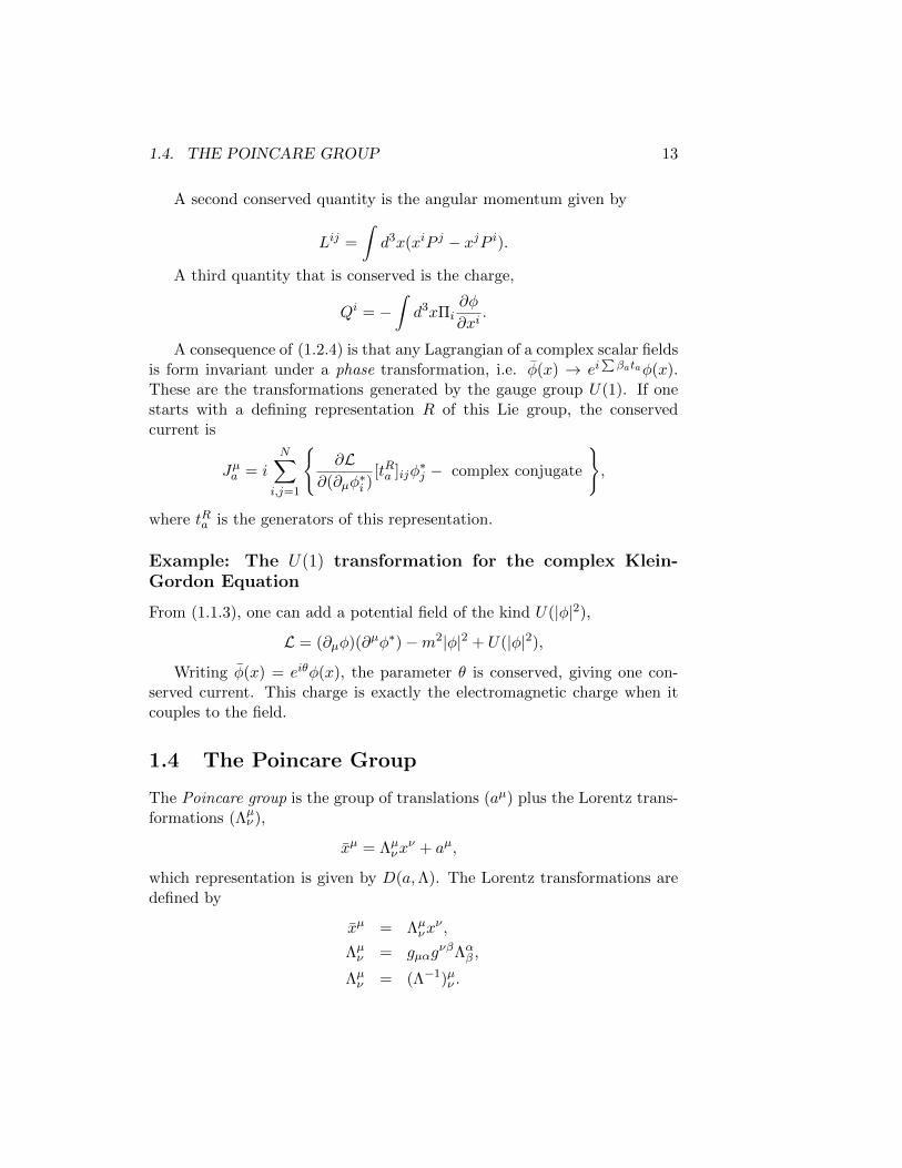
A second conserved quantity is the angular momentum given by
Lij =
∫d3x(xiP j − xjP i).
A third quantity that is conserved is the charge,
Qi = −∫d3xΠi
∂φ
∂xi.
A consequence of (1.2.4) is that any Lagrangian of a complex scalar fieldsis form invariant under a phase transformation, i.e. φ(x) → ei
∑βataφ(x).
These are the transformations generated by the gauge group U(1). If onestarts with a defining representation R of this Lie group, the conservedcurrent is
Jµa = iN∑
i,j=1
∂L
∂(∂µφ∗i )[tRa ]ijφ
∗j − complex conjugate
,
where tRa is the generators of this representation.
Example: The U(1) transformation for the complex Klein-Gordon Equation
From (1.1.3), one can add a potential field of the kind U(|φ|2),
L = (∂µφ)(∂µφ∗)−m2|φ|2 + U(|φ|2),
Writing φ(x) = eiθφ(x), the parameter θ is conserved, giving one con-served current. This charge is exactly the electromagnetic charge when itcouples to the field.
1.4 The Poincare Group
The Poincare group is the group of translations (aµ) plus the Lorentz trans-formations (Λµν ),
xµ = Λµνxν + aµ,
which representation is given by D(a,Λ). The Lorentz transformations aredefined by
xµ = Λµνxν ,
Λµν = gµαgνβΛαβ ,
Λµν = (Λ−1)µν .

14 CHAPTER 1. SPIN ZERO
The six generators (δλ) are found near the identity
Λµν = δµν + δλµν , (1.4.1)
= (I + δλ)µν , (1.4.2)
where in general the determinant of Λ is 1. This matrix can be writtenexplicitly for a representation with a rotating term and then a boost as
Λµν = (eiω.ke−iθ.j)µν .
The generators of the Poincare group in the representation of the fieldsφb are
(pµ)ab = −iδab∂µ.(mµν)ab = −iδab(xµ∂ν − xν∂µ)− (Σµν)ab,
with an algebra given by[pµ, pν ] = 0,
[pµ, mλγ ] = igµλpσ − igµσpλ,
[mµν , mλν ] = igµλmνσ + 3 terms.
1.5 Quantization of Scalar Fields
To start the quantization of the fields φ and its conjugate momentum Π,one postulates the basic equal-time commutators (ETCRS),
[φ(x, x0),Π(y, x0)] = i~δ3(x− y), (1.5.1)
[φ∗(x, x0),Π∗(y, x0)] = −i~δ3(x− y), (1.5.2)
[φ(x, x0), φ(y, x0)] = [Π(x, x0),Π(y, x0)] = 0. (1.5.3)
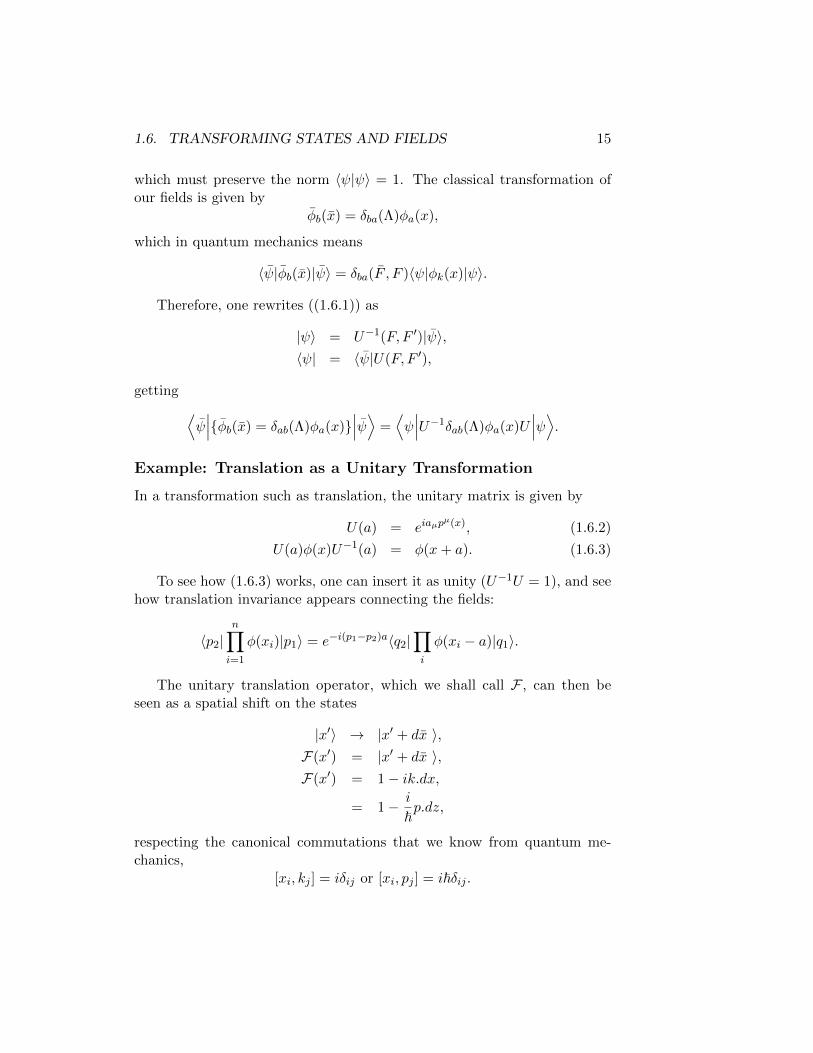
1.6 Transforming States and Fields
To see how one transforms states and fields, let us suppose the system inthe frame F , with states |ψ〉. In the frame F , with states |ψ〉, one needs tofind a unitary transformation U−1 = UT such as
|ψ〉 = U(F, F ′)|ψ〉, (1.6.1)
1.6. TRANSFORMING STATES AND FIELDS 15
which must preserve the norm 〈ψ|ψ〉 = 1. The classical transformation ofour fields is given by
φb(x) = δba(Λ)φa(x),
which in quantum mechanics means
〈ψ|φb(x)|ψ〉 = δba(F , F )〈ψ|φk(x)|ψ〉.
Therefore, one rewrites ((1.6.1)) as
|ψ〉 = U−1(F, F ′)|ψ〉,〈ψ| = 〈ψ|U(F, F ′),
getting ⟨ψ∣∣∣φb(x) = δab(Λ)φa(x)
∣∣∣ψ⟩ =⟨ψ∣∣∣U−1δab(Λ)φa(x)U
∣∣∣ψ⟩.Example: Translation as a Unitary Transformation
In a transformation such as translation, the unitary matrix is given by
U(a) = eiaµpµ(x), (1.6.2)
U(a)φ(x)U−1(a) = φ(x+ a). (1.6.3)
To see how (1.6.3) works, one can insert it as unity (U−1U = 1), and seehow translation invariance appears connecting the fields:
〈p2|n∏i=1
φ(xi)|p1〉 = e−i(p1−p2)a〈q2|∏i
φ(xi − a)|q1〉.
The unitary translation operator, which we shall call F , can then beseen as a spatial shift on the states
|x′〉 → |x′ + dx 〉,F(x′) = |x′ + dx 〉,F(x′) = 1− ik.dx,
= 1− i
~p.dz,
respecting the canonical commutations that we know from quantum me-chanics,
[xi, kj ] = iδij or [xi, pj ] = i~δij .

16 CHAPTER 1. SPIN ZERO
1.7 Momentum Expansion of Fields
We have now our fields quantized and we can work on the momentum ex-pansion of the fields. This involves their Fourier transformations
φ(k, x0) =
∫d3xe−ikxφ(x, x0),
Π(k, x0) =
∫d3xe−ikxΠ(x, x0).
It is necessary to write our φ and Π in terms of the creation/annihilationoperators (such as when we do it for x and p in quantum mechanics, definingthe raising/lowering operators), as can be seen in (1.7.1),
a(k, x0) =1
(2π)3/2
(ωkφ(k, x0) + iΠ(k, x0)
)
a†(k, x0) =1
(2π)3/2
(ωkφ(k, x0)− iΠ(k, x0)
) (1.7.1)
where ωk =√k2 +m2, which is the on-shell energy equation4 E2 =
p2 +m2. The four-vector notation can be written as kµ = (ω,~k).From the definition of the ETCR given by (1.5.1), (1.5.2) and (1.5.3),
one can then computes the ETCRs for (1.7.1), 3
[a(k, x0), a†(k, x0)] = 2~ωkδ3(k − k′), (1.7.2)
[a, a] = [a†, a†] = 0. (1.7.3)
Using ((1.7.1)) to rewrite the fields in terms of the creation/annihilationoperators, we have
φ(x, x0) =
∫d3k
(2π)3/22ωk[a(k, x0)eikx + a†(k, x0)e−ikx],
Π(x, x0) = −i∫
d3k
(2π)3/22[a(k, x0)eikx − a†(k, x0)e−ikx].
(1.7.4)
Substituting (1.7.4) in the Hamiltonian for scalar fields, one gets
H =1
4
∫d3k[a(k, x0)a†(k, x0) + a†(k, x0)a(k, x0)]. (1.7.5)
3Setting c = 1, the natural unit.

1.8. STATES AND FOCK SPACE 17
A remarkable characteristic of the free fields is the fact that the La-grangian is quadratic in fields, as you can see in (1.7.5). Making use of thetemporal evolution of the fields, one can calculate the commutation of thecreation/annihilation operator with this Hamiltonian,
[H, a(k, k0)] = −da(k, x0)
dt= ωka(k, x0).
1.8 States and Fock Space
The Fock Space is defined by the kets |k1〉, where all states are found byapplying the raising/creation operators from the ground states. Considering
|E′〉 = a†(k)|E〉,
one computes
H|E′〉 = Ha†(k)|E〉,= [H, a†(k)]|E〉+ a†(k)H|E〉,= ωka
†(k)|E〉+ Ea†(k)|E〉,= (E + ωk)|E′〉,
which clearly shows the shift on the energy when one applies the Hamiltonianoperator on some eigenstate. Requiring that the system has a ground state|0〉 allows
a(k)|0〉 = 0,
Therefore, it is possible to define the following states as
|k1, ..., kn〉 =n∏i=1
a†(ki)|0〉,
and applying the Hamiltonian operator, one finally has
H|k1, ..., kn〉 =∑i=1
ω(ki)|k1, ..., kn〉.
The dimension of the space is given by F = F0 ⊕ F1 ⊕ ... ⊕ FN , whereN in F is determined by the number operator,
N =
∫d3k
2ωka†(k)a(k), (1.8.1)
N( N∏i=1
a†(ki)|0〉)
= n( N∏i=1
a†(ki)|0〉). (1.8.2)

18 CHAPTER 1. SPIN ZERO
It is necessary to normal order N , i.e. relocate all a’s right to a†’s. Fromthis, one can rewrites the Hamiltonian (1.7.5) as
H|0〉 =1
4
∫d3k [a(k), a†(k)]|0〉,
= δ3(0)
∫d3k
ωk2δ3(0),
where the delta function is defined as
δ3(k − k′) =
∫d3x
(2π)3e−ix(k−k′). (1.8.3)
The normal ordered Hamiltonian is then given by
: H :=1
2
∫d2k a†(k)a(k). (1.8.4)
: H : |a〉 = 0. (1.8.5)
From these results, an important completeness relation is given by
1 = |0〉〈0|+∫
d3k
2ωk|k〉〈k|+ 1
2
∫d3k1d
3k2
2ωk2ωk1|k1k2〉〈k1k2|.... (1.8.6)
1.9 Scattering and the S-Matrix
The theory we have been developed should be used to calculated the simplestprocess on field theories, a particle scattering. In such process there will aninitial state, IN, which we say that is very far before the scattering moment,and a final state, OUT, taken a long time after the scattering moment. Onceone assumes completeness of these both states and waiting long enough, anystate will constitute a superposition of separable particles. Quantitativelyone may say that
• All particles were separated:∑
σ |αin〉〈αin| = 1.
• All particles are eventually separated:∑
σ |βout〉〈βout| = 1.

1.9. SCATTERING AND THE S-MATRIX 19
The S-matrix is the amplitude for a system that was simple in the pastand which will be simple in the future, and is defined by
Sαβ = 〈βout|αin〉,
with the following proprieties,
1. Completeness: S is unitary.
2. T-matrix: another unitary matrix can be obtained by S = 1 + iT .
3. Probabilistic interpretation: the process β → α has the probability|Sαβ|2, and α→ β, |Sβα|2.
Causal Green’s Function
The Green’s functions are connective solutions for equations of the type
(2x +m2)G(x− x′) = δ4(x− x′),
which the solutions with sources are
(2x +m2)φ = J.
In the scalar field Lagrangian such as (1.1.3), one can insert an additionalquadratic term which represents the fields acting on itself
L = |∂φ|2 −m2φ2 − λ(|φ2|)2.
For such a problem, the solution of the equation of motion can be givenby the causal Green’s function
(k2 −m2)G(k) = 1,
G(k) =
∫d4xe−i(k−k
′)G(x− x′),
G(k) =1
k2 −m2.
The Green’s function has an important role on field theory, this con-nection propriety ultimately will be used to represent transition amplitudebetween states,
G(x1, ..., xN ) = 〈0|Tφ(x)...φ(xn)|0〉. (1.9.1)

20 CHAPTER 1. SPIN ZERO
The Reduction Theorem
The reduction theorem relates the Green’s function for states, (1.9.1) to theS-Matrix
S(qj , ki) = 〈qjout|kiin〉,
S(qj , ki) =1(
i(2π)32R)n+m
∣∣∣∣∣n∏j=1
(q2j −m2
j )
m∏i=1
(k2i −m2
i )G(qi − ki)
∣∣∣∣∣k2i=m2
i ,q2i=m2
i
,
where R = (2π)3|〈0|φ(0)|ρ〉|2. In each isolated particle, G has a separatedpole and the residue is S. The construction is possible by considering a largetime where the wave are isolated particles.
1.10 Path Integral and Feynman Diagrams
To start the study of Path Integral, we need to define the concept of station-ary phase, which is the previous transition amplitude as the product of allpossible trajectories for two classical coordinates q′ and q′′,
U(q′′, t′′, q′, t′) = 〈q′′, t′′|q′, t′〉,
= limn→∞
(m
2πiδt~
)n2 n∏i=1
∫dqie
1~∑j δtL(qk,qj).
The stationary phase integral for the path integral, in the semi-integralapproximation, is given by the classical variations. We can, define the gen-erating function of q(t) as
Z[J ] =
∫ q2
q1
[dq]e1~ [S−
∫ t′′t′ dtJ(t)q(t)] (1.10.1)
The transition for fields is made by the formal substitution∫
[dp][dq]→∫[dπ][dφ], which can have the interpretation of transforming one harmonic
oscillator to infinite number of harmonic oscillators, all labeled by their wavenumber k. The generating are then
Wδa[J(xµ)] =
∫[dφ]e
i~∫d4x 1
2[SL′−
∫d4xJ(x)φ(x)],
=
∫[dφ]e
i~∫d4x 1
2[(∂µφ)2−m2φ2−J(x)φ(x)],

1.10. PATH INTEGRAL AND FEYNMAN DIAGRAMS 21
where the last term can be seen as a charge source.Let us recall the procedure of Wick’s rotation , which is the method of
finding a solution to a problem in Minkowski space from a solution to arelated problem in Euclidean space. The Wick’s rotation consists in per-forming the transformation t→ iτ , making it on W [J ] for the single degreeof freedom. From t[y] = e−iθτ , 0 < θ < π
2 , it is possible to write W [J ] =lim θ→0+W [J, θ]. From ((1.10.2)), it is possible to construct the free fieldGreen’s functions from the transition amplitude,
〈0|T (φ(x)φ(y)|0〉 = i∆f (x− y),
where the original equation of motion can be written as the
(2x +m2)∆f (x− y) = −δ4(x− y),
where Euclidean delta function is
i∆f (x) =
∫d4k
(2π)4
e−ikx
k2 −m2 + iε.
The Green’s function, from i terms of the generating functional, equation(1.10.2), is then
GN (x1, ..., xn) =⟨
0∣∣∣T( n∏
φ(xi))|0⟩, (1.10.2)
= (i~)nn∏i=1
δ
δJ(xi)Wδ0 [J ], (1.10.3)
where
Wδ0 [J ] = ei2~
∫d4zd4yJ(z)∆p(z−y)J(y). (1.10.4)
Equation (1.10.4) gives the Feynman Rules for scalars fields, summarizedas
1. Write all possible distinguished graphics for the process.
2. For each line, associate the propagator∫
d4k(2π)4
1k2−m2+iε
.
3. For each vertex associate −ig(2π)4g4δ(∑
i Pi−∑
j kj), where the deltafunction is over the sum of the momenta that come to the vertex.

22 CHAPTER 1. SPIN ZERO
Chapter 2
Fields with Spin
A more realistic kind of field theories are those that obey the spin-statistictheorem, where all particles have either integer spin, bosons, or half-integerspin, fermions, in units of the Planck constant ~.
2.1 Dirac Equation and Algebra
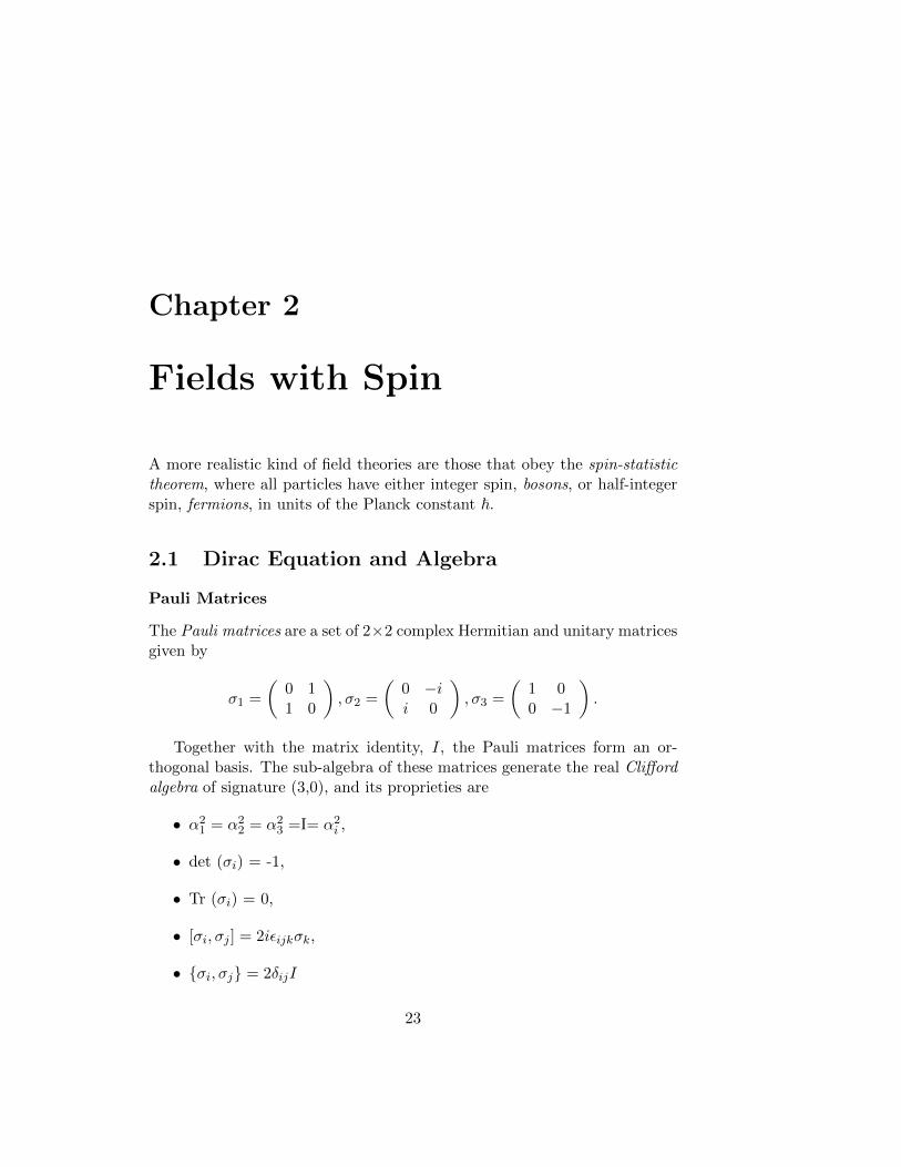
Pauli Matrices
The Pauli matrices are a set of 2×2 complex Hermitian and unitary matricesgiven by
σ1 =
(0 11 0
), σ2 =
(0 −ii 0
), σ3 =
(1 00 −1
).
Together with the matrix identity, I, the Pauli matrices form an or-thogonal basis. The sub-algebra of these matrices generate the real Cliffordalgebra of signature (3,0), and its proprieties are
• α21 = α2
2 = α23 =I= α2
i ,
• det (σi) = -1,
• Tr (σi) = 0,
• [σi, σj ] = 2iεijkσk,
• σi, σj = 2δijI
23
24 CHAPTER 2. FIELDS WITH SPIN
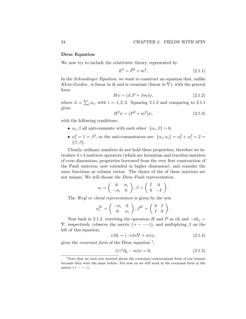
Dirac Equation
We now try to include the relativistic theory, represented by
E2 = ~P 2 +m2, (2.1.1)
In the Schroedinger Equation, we want to construct an equation that, unlikeKlein-Gordon , is linear in ∂t and is covariant (linear in ∇), with the generalform
Hψ = (~α.P + βm)ψ, (2.1.2)
where ~α =∑
i αi, with i = 1, 2, 3. Squaring 2.1.2 and comparing to 2.1.1gives
H2ψ = (P 2 +m2)ψ, (2.1.3)
with the following conditions:
• αi, β all anti-commute with each other: αi, β = 0.
• α2i = 1 = β2, so the anti-commutators are: αi, αi = α2
i + α2i = 2 =
β, β.
Clearly, ordinary numbers do not hold these proprieties, therefore we in-troduce 4×4 matrices operators (which are hermitian and traceless matricesof even dimensions, proprieties borrowed from the very first construction ofthe Pauli matrices, now extended in higher dimension), and consider thewave functions as column vector. The choice of the of these matrices arenot unique. We will choose the Dirac-Pauli representation,
αi =
(0 σi−σi 0
), β =
(I 00 −I
).
The Weyl or chiral representation is given by the sets
αWi =
(−σi 0
0 σi
), βW =
(0 II 0
).
Now back in 2.1.2. rewriting the operators H and P as i∂t and −i∂xi =∇, respectively (observe the metric (+ − −−)), and multiplying β on theleft of this equation,
iβ∂t = (−iβα∇+m)ψ, (2.1.4)
gives the covariant form of the Dirac equation 1,
(iγµ∂µ −m)ψ = 0, (2.1.5)
1Note that we were not worried about the covariant/contravariant form of our tensorsbecause they were the same before. For now on we will work in the covariant form in themetric (+ −−−).

2.1. DIRAC EQUATION AND ALGEBRA 25
with the inclusion of the four Dirac matrices γµ = (β, βαi).
Clifford Algebra
From the constrains that we have found for β and αi, we are going to derivethe algebra of the Dirac matrices, the Clifford algebra. First, let us resumethem in
αi, αj = 2δij and β, β = 2 and αi, β = 0.
It is clear that introducing a four-vector notation will summarize them.Let us from this derive the algebra of a four-vector representation γµ =(β, βαi), testing all possibilities of commutations. For i 6= j,
β, βαj = ββαi + βαiβ
= β2αi − αiβ2
= 0.
βαi, βαj = βαiβαj + βαjβαi
= −αiβ2αj − αjβ2αi
= αi, αj,= 0.
β, β = β2 + β2,
= 2.
Now, for i = j,
βαi, βαi = βαiβαi + βαiβαi,
= 2βαiβαi,
= −2αiββαi,
= −2.
Rewriting all in terms of γ-matrices,
β = γ0,
βα1 = γ1,
βα2 = γ2,
βα3 = γ2,
we can see clearly that
γ0, γ0 = 2,
γ0, γi = 0,
γi, γj = −2δij ,

26 CHAPTER 2. FIELDS WITH SPIN
Resulting, finally, in the Clifford Algebra,
γµ, γν = γµγν + γνγµ = 2gµν , (2.1.6)
where gµν is the element of the metric with the signature (+,−,−,−).We can prove 2.1.6 explicitly by actually substituting the Pauli matrices
into γµ = (β, βαi). For example, for γ0, γ2,
(I 00 −I
)(0 σ2
−σ2 0
)=
1 0 0 00 1 0 00 0 −1 00 0 0 −1
0 0 0 −i0 0 i 00 i 0 0−i 0 0 0
= 0,
and for γ3, γ3,
(0 σ3
−σ3 0
)(0 σ3
−σ3 0
)=
0 0 1 00 0 0 −1−1 0 0 00 1 0 0
0 0 1 00 0 0 −1−1 0 0 00 1 0 0
= −2.
2.2 Spinors
Recalling equation (1.4.1), one can write the general space-time transforma-tions of fields as
φa(x) = Sab(Λ)φb(Λ−1x− a),
which, near to the identity, can be writen as
Sab(1 + δλ) = δab +1
2iδλµν(Σµν)ab.
The matrices S(Λ) must obey the Poincar group proprieties S(Λ1)S(Λ2) =S(Λ1,Λ2). The fields φb are tensors that transform according to the repre-sentation on S(Λ). In quantum field theory the transformations are unitary,therefore the representation of the Poincare groups is given by the matrices
Λµν = eiω.Ke−θ.J = S(Λ), (2.2.1)
resulting on the Lorentz transformations of the fields,
U(a,Λ)φa(x)U−1(a,Λ) = Sab(Λ−1)φb(Λx+ a). (2.2.2)

2.2. SPINORS 27
With the transformation matrices established, it is possible to constructthe algebra for the Poincare group on field theory. The Poincare algebra,(1.4.3), gives the Lie algebra for the generators K and J on (2.2.1),
[Ja, Jb] = iεabcJc,[Ka,Kb] = −iεabcJc,[Ja,Kb] = iεabcKc.
(2.2.3)
Setting the normalization T (j) = 12 such that tr ta, tb = T (j)δab, with
j labeling an irreducible representation(irrep) of SU(2), one can write theCasimir operators in terms of the generators,
3∑a=1
[t(j)a ]2 = j(j + 1)Ij ,
Let us consider the Pauli matrices, defined as
σ0 = 1 =
(1 00 1
), σx = σ1 =
(0 11 0
),
σy = σ2
(0 −ii 0
), σ3 = σz =
(1 00 −1
).
A representation for the Lorentz group for 2 × 2 system in the gaugegroup Sl(2, C), can be writen, and it is called spinors,
Ka = −1
2iσa,
Ja =1
2σa,
Ka =1
2iσ∗a,
Ja =1
2σ∗a.
(2.2.4)
Substituting (2.2.4) back on (2.2.1), one has
h(Λ)ab = (eω.σ2 e−iθ.
σ2 )ab ,
h∗(Λ)ab
= (eω.σ∗2 e−iθ.
σ∗2 )a
b,
(2.2.5)
where a, a runs from 1, 2, and in this representation, h−1(Λ) = h(Λ−1).Therefore, the spinor representation is double valued. For instance, for

28 CHAPTER 2. FIELDS WITH SPIN
rotation only one has h∗(R) = σ2h(R)σ2, which is not necessary truewhen adding a boost.
The relation between h(Λ) to Λµν from (2.2.1) and (2.2.5) is convention-ally given by taking the trace
Λµν =1
2Tr [σµh(Λ)σνh
†(Λ)], (2.2.6)
where σµ = (σ0, ~σ). A rotational spinor ηa = (η1, η2) is defined as a complexobject that transform on the following way
ηb = h(Λ)baηa, (2.2.7)
ξb = h∗(Λ)baξa. (2.2.8)
They are the Weyl spinors and they give scalars by constructing
ηa = εabηb,
ξa = εabξb,
where
εab = εab =
(0 1−1 0
),
and
εab = εab = −εab.
These matrices are characteristic in the symplectic Lie groups and trans-form with the Pauli matrices as εσiε
−1 = −σTi . From this, one has
ηa = [h−1(Λ)]caηc
= ηc[h(Λ)]ca,
ξa = [h∗−1(Λ)T ]caξc
= ξc[h∗(Λ)]ca.
Applying this last resulting in the previous calculation to find the scalarsof the theory, one finds ηaη
a = ηaηa, (ξa)∗ηa, and (ηa)
∗ηa.
2.3. VECTORS 29
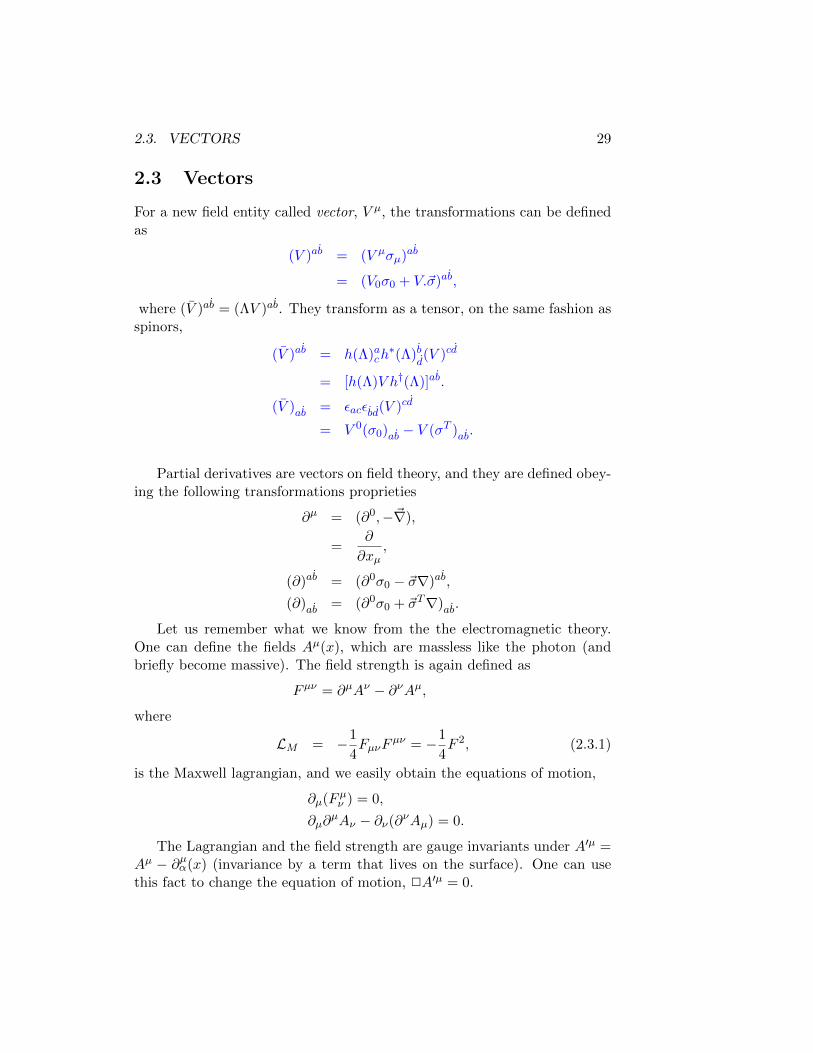
2.3 Vectors
For a new field entity called vector, V µ, the transformations can be definedas
(V )ab = (V µσµ)ab
= (V0σ0 + V.~σ)ab,
where (V )ab = (ΛV )ab. They transform as a tensor, on the same fashion asspinors,
(V )ab = h(Λ)ach∗(Λ)b
d(V )cd
= [h(Λ)V h†(Λ)]ab.
(V )ab = εacεbd(V )cd
= V 0(σ0)ab − V (σT )ab.
Partial derivatives are vectors on field theory, and they are defined obey-ing the following transformations proprieties
∂µ = (∂0,−~∇),
=∂
∂xµ,
(∂)ab = (∂0σ0 − ~σ∇)ab,
(∂)ab = (∂0σ0 + ~σT∇)ab.
Let us remember what we know from the the electromagnetic theory.One can define the fields Aµ(x), which are massless like the photon (andbriefly become massive). The field strength is again defined as
Fµν = ∂µAν − ∂νAµ,
where
LM = −1
4FµνF
µν = −1
4F 2, (2.3.1)
is the Maxwell lagrangian, and we easily obtain the equations of motion,
∂µ(Fµν ) = 0,
∂µ∂µAν − ∂ν(∂νAµ) = 0.
The Lagrangian and the field strength are gauge invariants under A′µ =Aµ − ∂µα(x) (invariance by a term that lives on the surface). One can usethis fact to change the equation of motion, 2A′µ = 0.

30 CHAPTER 2. FIELDS WITH SPIN
2.4 Majorana Spinors
One of first attempts of adding a mass term for the two-component spinorswas done by the Majorana, called Majorana spinors. Weyl equations aremassless and Dirac equations require that the spinors are indistinguishable,resulting on the Majorana Lagrangian
LM = (η∗)b(∂)abηa +
m
2(ηaη
a + η∗aη∗a),
with the the Majorana equation of motion
(∂)abηa +m(η∗)b = 0,
which is not consistent to the U(1) symmetry, i.e. the phase symmetry.
2.5 Weyl Equation and Dirac Equation
The spinors we had previously defined have to satisfy the Klein-Gordonequation, (1.1.2),(2 + m2)ηa(x) = 0. When we make m = 0 we obtain themassless equation called Weyl equation. For the component spinors ηa(x),one has
(∂)abηa(x) = 0,
multiplying by (∂)cb = (σ0∂0 − σ.∇)cb,
one has 2ua(x) = 0.
One can also derive the Weyl equation from the Lagrangian densityL = u∗b(∂)abu
a, which is a Lorentz scalar. The generalization of the Weylequation, when one includes mass, is called Dirac equation, to construct theDirac equation, one defines one more spinor ξa such as in the table 2.5.
ηa(x)→ Transforms as h(Λ)ξa(x)→ Transforms as [h−1(Λ)]†
Table 2.1: Spinor transformation in the Dirac/Weyl theory.
The two components are linked to the two spinors as
i(∂)cbηc(x)−mξb(x) = 0,
i(∂)adξd(x)−mηd(x) = 0,

2.5. WEYL EQUATION AND DIRAC EQUATION 31
which can be written as a matrix in terms of σµ(−mδd
bi(σ0∂
0 + σ∇)bci(σ0∂
0 + σ∇)ad −mδca
)·(ξd(x)ηc(x)
)= 0,
The Dirac spinor representation in the 4× 4 notation is
ψ(x)D =
(ηa + ξa
ηb − ξb
),
which transforms with the Dirac matrices
γiD
(0 σi−σi 0
), γ0D
(σ0 00 −σ0
).
The Weyl or chiral representation is given by the sets
ψ(x)W =
(ξd(x)ηc(x)
),
these 4 × 4 four-component spinors representation also transform by theDirac matrices
γiW
(0 σi−σi 0
), γ0W
(0 σ0
σ0 0
).
The Dirac equation can be written as
(i∂µγµ −m)ψ(x) = 0, (2.5.1)
where one defines
ψ(x) = ψ†γ0,
= (ψ∗)Tγ0,
and the Lorentz invariant is
(ψψ) = ψαψα
= (ξa)∗ηa + (ηa)∗ξa.
The Dirac Lagrangian is
L = ψ(i∂µγµ −m)ψ. (2.5.2)

32 CHAPTER 2. FIELDS WITH SPIN
From unitary transformations we can write another representation,
ψ′ = Uψ,
γ′µ = UγU−1,
where
U =1√2
(σ0 σ0
−σ0 σ0
).
The basic proprieties of the Dirac’s matrices algebra, which is the CliffordAlgebra, is given by the anticommutation of two matrices,
γµ, γν = γµγν + γνγµ (2.5.3)
= 2gµν(I4×4), (2.5.4)
where, for the 4× 4 representation, one has the possible representations inthe table 2.2.
Number of γ 0 1 2 3 4Element I γµ σµν γµγ5 γ5
Quantity 1 4 6 4 1
Table 2.2: The Clifford matrices for the 4× 4 representation.
2.6 Lorentz Transformations
As we have seen on (1.4.2) and (2.2.1), in general, near to the identity, onecan write the generators of the group, such as the Lorentz group, in the formof the expansion
Sab(1 + δλ) = I +1
2iδλ(Σµν)ab. (2.6.1)
In the case of Dirac’s equation, conventionally one has
(Σµν)αβ = −1
2(σµν)αβ, (2.6.2)
where the new tensor is defined as
σµν =i
2[γµ, γν ],

2.7. SYMMETRIES OF THE DIRAC LAGRANGIAN 33
with the following commutation relation to γρ,
[σµν , γρ] = 2i(gνργµ − gµργν).
Hence, it is possible to rewrite equation (2.6.1) as
S(1 + δλ) = I − 1
4iδλ(σµν), (2.6.3)
where the finite transformation is as an arbitrary boost plus an arbitraryrotation,
S(Λ)αβ = [e12ωiσ0ie−
14θiεijkσjk ]αβ. (2.6.4)
Finally, we have the following important relations with the Dirac’s ma-trices,
S†(Λ)γ0 = γ0S−1(Λ),
S−1(Λ)γµS(Λ) = Λµνγµ,
Λµα∂α = ∂µ.
2.7 Symmetries of the Dirac Lagrangian
The Dirac Lagrangian, given by (2.5.2), can be written in a more compactway in the slash-notation, where 6∂ = γµ∂
µ,
LD = ψ(i6∂ −m)ψ,
This Lagrangian is invariant under the gauge groups SU(N) and U(1).
Noether’s Theorem
In the same fashion as the theory for scalar fields, one can define the con-served current, (2.7.1), for spinors
Jαa = −
(∂(δxα)
∂βa
)L −
∑i
∂L∂(∂aφi)
∂δ∗φi∂βa
,
where a is the parameter of transformation, α the vector index, the Poincareterms are βaδx
µ, δλµν , and the last term is the variation at a point. Looking

34 CHAPTER 2. FIELDS WITH SPIN
to the form of the change of a field on a point on the Dirac’s theory, one has
δxα = δaα +1
2δλαµx
µ,
δ∗φi(x) = −(δνagµν − δλνµδxν)
∂φi(x)
∂xµ− i
2(Σµν)ijδλ
µνφj(x),
where, from (2.6.2) we know that (Σµν)αβ = 12(σµν)αβ, and the last part of
this equation is a new term different from the scalar theory. The Noether’scurrent is
HD =
∫d3x T00
D ,
=
∫d3x(−L+ iψ†∂0ψ),
=
∫d3xψ(−iγ∇+m)ψ.
The conjugate momenta in the Dirac’s theory is
Πα =∂L∂ψα
= iψ†α, (2.7.1)
and the momentum-energy tensor is
δaµ :∂
∂(δaµ)→ Tµα.
δλµν :∂
∂(δλµν)→Mµνα.
The quantities Pν =∫d3xT0ν and Jνλ =
∫d3xM0νλ have the usual
interpretation as the total momentum and the angular momentum tensor,
Jνλ =
∫d3xMνλ0 ,
=
∫d3x(xνT0λ − xλT0ν) + i
∫d3xΠi(Σνλ)ijφj ,
where the second term is the spin/intrinsic angular momentum, and Πi, φjare the fields ψ’s. The new contribution describes the intrinsic spin and ameasure of it is give by the Pauli-Lobanski vector, :
Wµ = −1
2εµνλσJ
νλP σ,
= −1
2iεµνλσ
∫d3xΠi(Σνλ)ijφjP
σ,

2.7. SYMMETRIES OF THE DIRAC LAGRANGIAN 35
where W 2 = WµWµ and P 2 = PµPµ are Casimir operators of the theory .P 2 commutes with W 2, eigenvalues of Wµ. In the rest frame, the momentumvector reduces to a 3-vector, while in the other frames WµPµ = 0.
Global Symmetries
The group of the global symmetries is U(N) = U(1) × SU(N). We canconstruct such symmetry by replicating fields with same mass
L =N∑i−1
(ψi)α(i6∂ −m)αβ(ψi)β.
The Lagrangian is invariant by the transformation of (ψi)α,i = 1, ..., N ,
under eiθ (U(1)) and ei∑N2−1a=1 βaTa (SU(N)). This form-invariance produces
conserved currents and charges, from the Noether’s theorem,
Jµ =∂L
∂(∂αψi)δ∗ψi,
U(1) → Jα = ψγµψ,
SU(N) → Jαa = ψγµTaψ,
Qa =
∫d3xJ0
a .
Parity
If ψ(x) solves the Dirac equation, so does γ0ψ(x) = ψ(x0,−x). In the Weylnotation, the γ0 exchanges the position of the dotted by the undotted andfor this reason the Weyl Lagrangian ] density is not form invariant underparity transformation.
A fifth gamma matrix is defined as
γ5 = iγ0γ1γ2γ3 =i
4!εµνλσγ
µγνγλγσ. (2.7.2)
γ5, γµ = 0.
γW5 =
(−σ0 0
0 σ0
)γD5 =
(0 σ0
σ0 0
)

36 CHAPTER 2. FIELDS WITH SPIN
From this new matrix γ5, one can define the projective operators , thatproject out states in the Weyl representation. The so-called chiral represen-tation is given by
1
2(1− γ5)ψ =
(ξd0
)→ Left− handed.
1
2(1 + γ5)ψ =
(0ηc
)→ Right− handed.
2.8 Gauge Invariance
One of the most important gauge fixing is the Lorentz gauge given by
∂µAµ = 0.
It is possible to impose it from the beginning by modifying the MaxwellLagrangian itself
LM (A, λ) = −1
4FµνF
µν − 1
2λ(∂µA
µ),
This is no longer gauge invariant. Acting ∂ν on 2Aν−(1−λ)∂ν(∂A) = 0results in λ2(∂A) = 0.
Proca Field
The Proca field is the generalization of a massive vector field. The La-grangian is given by the Maxwell Lagrangian plus a mass term on the vectorfields
LP = −1
4FµνF
µν +m2AµAµ, (2.8.1)
with equation of motion
∂µ∂µAν − ∂ν(∂µAµ) +m2Aν = 0.
If one acts ∂ν on this equation, it is possible to get the Lorentz conditionback, which is Lorentz invariant, such as the Klein-Gordon equation. Sinceit is not possible to remove the third number of degree of freedom, the Proca
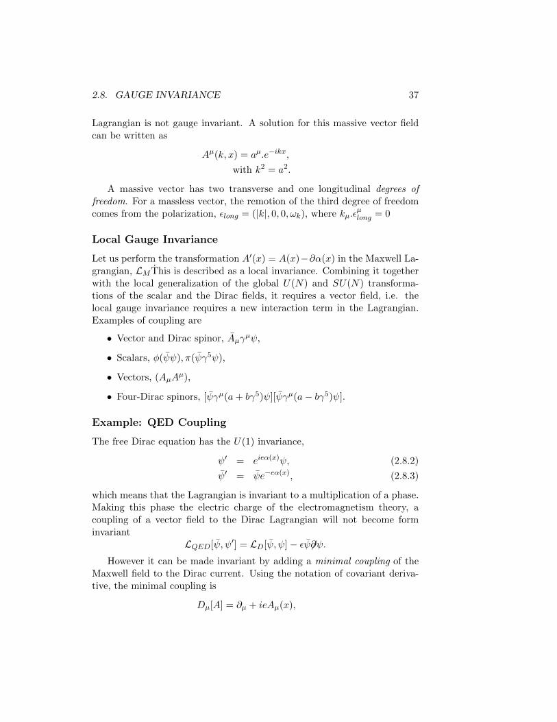
2.8. GAUGE INVARIANCE 37
Lagrangian is not gauge invariant. A solution for this massive vector fieldcan be written as
Aµ(k, x) = aµ.e−ikx,
with k2 = a2.
A massive vector has two transverse and one longitudinal degrees offreedom. For a massless vector, the remotion of the third degree of freedomcomes from the polarization, εlong = (|k|, 0, 0, ωk), where kµ.ε
µlong = 0
Local Gauge Invariance
Let us perform the transformation A′(x) = A(x)−∂α(x) in the Maxwell La-grangian, LM This is described as a local invariance. Combining it togetherwith the local generalization of the global U(N) and SU(N) transforma-tions of the scalar and the Dirac fields, it requires a vector field, i.e. thelocal gauge invariance requires a new interaction term in the Lagrangian.Examples of coupling are
• Vector and Dirac spinor, Aµγµψ,
• Scalars, φ(ψψ), π(ψγ5ψ),
• Vectors, (AµAµ),
• Four-Dirac spinors, [ψγµ(a+ bγ5)ψ][ψγµ(a− bγ5)ψ].
Example: QED Coupling
The free Dirac equation has the U(1) invariance,
ψ′ = eieα(x)ψ, (2.8.2)
ψ′ = ψe−eα(x), (2.8.3)
which means that the Lagrangian is invariant to a multiplication of a phase.Making this phase the electric charge of the electromagnetism theory, acoupling of a vector field to the Dirac Lagrangian will not become forminvariant
LQED[ψ, ψ′] = LD[ψ, ψ]− εψ 6∂ψ.However it can be made invariant by adding a minimal coupling of the
Maxwell field to the Dirac current. Using the notation of covariant deriva-tive, the minimal coupling is
Dµ[A] = ∂µ + ieAµ(x),
38 CHAPTER 2. FIELDS WITH SPIN
which allow us to write the QED Lagrangian
LQED(ψ, ψ,A) = ψ(i6D[A]−m
)ψ − 1
4F 2,
= ψ(i(∂µ + ieAµ)γµ −m
)ψ − 1
4F 2.
The quantum electrodynamic theory is then represented by the La-grangian
LQED = LD + (iεAµψγµψ). (2.8.4)
Method of Wigner
Wigner developed a method by which representations of the Poincare groupcan be constructed explicitly. We start with a eigenstate |p, λ〉 of P 2 where
Pµ|p, λ〉 = pµ|p, λ〉.
The operators versions of Pµ and Jµ generate unitary representations ofPoincare group, and one can treat Pµ and Jµ as hermitian operators on thespace of states.
Fixing p2 degenerates the basis states for all values of Pµ, and denotingthe special fixed vector by qµ, we have q2 = m2. Any vector Pµ with p2 = m2
can be derived by acting on qµ with the appropriate Lorentz transformationPµ = Λ(p, q)µνqν . The transformations is not unique, it can be modified toΛ(p, q) = Λ(p, q)l. The set of all transformations l that satisfies lq = q is agroup, the Wigner little group. The set of states with momentum qµ whichtransforms according to irreps of the little group are
U(l)|qµ, λ〉 =∑σλ
(l)|qµ, σ〉.
To find the representations of l, for example if m2 > 0, one choosesqµ = (m, 0) (vector at rest). The l is the rotation group and the states|qµ, σ〉 are most conveniently chosen with σ as the projector of the spinalong the fixed axis.
The ambiguity of the choice of Λ that takes qµ into pµ can be removed bymaking a specific choice of Wigner boost, Λ0(p, q), for each pµ. A exampleis making pµ 6= qµ and getting |pµ, λ〉 = U(Λ0(p, q)|qµ, λ〉.

2.8. GAUGE INVARIANCE 39
The case k = 0, pµ = (m, 0). We want the solution for the Dirac equation
(i6∂ −m)αβξ±β (q)e∓iq0x0 = 0,
which is (i(∓i)γ0q0 −m)αβξ±β (q) = 0.
In the matrix representation:((±q0 −m)σ0 0
0 −(±q0 −m)σ0
)ξ± = 0.
We find four independent solutions,
uα(q,±1
2)e−iqx, vα(q,±1
2)eiqx.
For instance, the two solutions are the positive energy and the two lastare the negatives,
uα(q,+1
2) = C
1000
,
where C is the normalization constant, here chosen to be C =√
2m.
The case k 6= 0, q 6= p. We want the solution
( 6q −m)ξ±β (λ) = 0,
S(Λ(p, q))6qS−1Λ(p, q) = 6p,
and the infinite solutions
( 6p−m)[S(Λ(p, q)ξ±(λ)] = 0.
We need a unitary transformations, however, in general, spinors trans-formations are non-unitary S(Λ), making it necessary to have
U(Λ)|k±, λ〉 =∑σ
Dλσ(Λ)|Λk±, σ〉,
where D†D = 1.
This equation requires then
U(Λ)b†λ(k)U(Λ−1) =∑σ
Dλσ(Λ)b†σ(Λk),
consistent to Uψ(x)U−1 = S(Λ−1)ψ(Λx).

40 CHAPTER 2. FIELDS WITH SPIN
Hence we construct a set of spinor solutions that transforms arbitraryby Dirac. In this case, the conservation of probability requires
U(Λ)b†U−1(Λ) =∑σ
Dλσ(Λ)b†σ(Λk).
Now let us look to Sαβ(Λ−1d (k, λ), where we use the Wigner boost to
define
uα(k, λ) = Sαβ(Λw(k, q))uβ(q, λ),
S(Λ−1)uα(k, λ) = S(Λ−1)Sαβ(Λw(k, q))uβ(q, λ).
However S(Λw(q, k′))S(Λ−1)S(Λw(k, q)) = S(Λw(q, k′)Λ−1Λw(k, q) =S(lk′,k,q) is a rotation! This results that
Sαβ(Λ−1)uβ(k, λ) =∑σ
Dλσ(lk′,k,q)uα(k′, σ),
=
∫dk∑λσ
bλ(Λk′)Dλσ(lk′,k,q)u(k′, σ)e−ikx,
with the equation insured by
U(Λ)bσ(k)U−1(Λ) =∑λ
bλ(Λk)Dλσ(lk′,k,q).
Finally, in resume, the two steps for finding these kind of solutions are
1. Define ((2.8.5)).
2. Label solutions by rotation (Wigner’s little group), which are inducedsolutions.
The Wigner’s method works for any field with q2 = m2. For q2 = 0,we should choose different reference momentum qµ, and it is possible do itfortachyons.
From here, it is easy to construct basis of solutions to Dirac equation:using the spin (helicity) basis, Λw(k, q) is a pure boost inp-direction with
Λ0(p, q) = eiωp.k,
ω = tanh−1( |p|√
p2 +m2
),
pµ = Λ0(p, q)µνqν ,
qµ = (m,~0)αβΛ0(p, q) = eiωp.k.
2.8. GAUGE INVARIANCE 41
To evaluate the solutions, we denote ω = u, v the spin basis
ω(p, λ) = S(Λ0(p, q))ω(q, λ),
where Sαβ(Λ0(p, q)) = e−14ωpi[γ0,γi]αβ
Evaluating this in the Dirac algebra gives
S(Λ0(p, q)) = e12ωp.α,
S(Λ0(p, q)) = I coshω
2+ φα sinh
ω
2,
and with a little algebra one gets the Dirac representations.
Sumating it up, the basis u and v can be written as:
u(p, λ) =1√
2m(p0 +m)(6p+m)u(q, λ),
v(p, λ) =1√
2m(p0 +m)(−6p+m)v(q, λ),
and it is possible to make also use of
S†(λ)γ0 = γ0S−1(Λ),
u(p, λ) =1√
2m(p0 +m)(−6p+m)u(q, λ),
v(p, λ) =1√
2m(p0 +m)( 6p+m)v(q, λ).
The final proprieties are
1. (6p−m)u = u(6p−m) = 0.
2. (6p+m)v = v( 6p+m) = 0.
3. The normalization of the scalars are u(p, λ)u(p, λ′) = |C|2δλλ′ , v(p, λ)v(p, λ′) =−|C|2δλλ′ .
4. The projector for u are∑
λ=± 12uλ(p, λ)uβ(p, λ) = |C|2
2m ( 6p + m)αβ, and
for v are∑
λ=± 12vλ(p, λ)vβ(p, λ) = |C|2
2m (6p−m)αβ .
42 CHAPTER 2. FIELDS WITH SPIN
2.9 Canonical Quantization
Making use of the spin representations, which are unitary representationsof the Poincare group, one can organizes fields in terms of solution to theclassical equation of motion,
1. Expanding to equation of motion.
2. Quantizating the coefficients.
3. Constructing the Hamiltonian H0.
4. Finding the x0-dependence of coefficients for free field.
5. Constructing the conserved charges.
From the classical transformations of the Dirac spinors, Sαβ(Λ)ψβ(x) =ψ′α(Λx) of, the expansion of the field has the general form (in the samefashion as we derived for scalar fields),
ψα(x) =∑λ
∫d3k
(2π)32 2ωk
[bλ(k)uα(k, λ)e−ikx + d†λ(k)vα(k, λ)eikx], (2.9.1)
where the Dirac spinors, uα, vα, are some bases of solution, and the trans-formations of the fields are given by
U(Λ)ψαU−1(Λ) = Sαβ(Λ−1)ψβ(Λx).
Quantization
Let us know understand (2.9.1). Due the fact that the Dirac Lagrangianis linear in derivatives, the canonical momentum of the field is simply itsconjugate, as in (2.7.1),
Π = iψα,
making the construction of the fields straightforward
ψα(x, x0) =
∫dkbλ(k, x0)uα(k, λ)eikx + dλ(k, x0)v∗α(k, λ)e−ikx,
Πα(x, x0) =
∫dkb†λ(k, x0)u†α(k, λ)e−ikx + dλ(k, x0)v†α(k, λ)eikx.
2.9. CANONICAL QUANTIZATION 43
The Hamiltonian of the theory is then
H0 =
∫d3xiψ†∂0ψ − ψ†γ0(iγ0∂0 + (iγ∇−m))ψ,
=
∫d3xψ−iγ∇+ γ0mψ,
=
∫d3k
1
2
∑λ
b†λ(k, x0)bλ(k, x0)− dλ(k, x0)d†λ(k, x0).
The Hamiltonian normal-ordered is
: H0 :=1
2
∑λ
∫d3kb†λ(k, x0)bλ(k, x0) + d†λ(k, x0)dλ(k, x0).
The canonical equal time anti-commutation relations are
b†λ(k, x0), bλ′(k′, x′0) = 2ωkδλλ′δ
3(k − k′),d†λ(k, x0), dλ′(k
′, x′0) = 2ωkδλλ′δ3(k − k′),
[bλ(k, x0), : H0 :] = ibλ(k, x0).
The states can be constructed by acting the raising/lowering operators
d(k, λ)|0〉 = b(k, λ)|0〉 = 0,
〈0|d† = 〈0|b† = 0.
andδi,j
∏i
b†λi(k′i)∏k
d†λj(kj)|0〉 = |k′i, λi, kj , λj〉,
where the delta has ± sign depending on the order of b and d. In the righthand side, the first term is the particle and the second is the antiparticle.The terms b† creates particles and d† creates antiparticles, and the differenceto the scalars is that now one has a antisymmetric wave function.
Momentum and Spin
In terms of creation/annihilation operators, the momentum is just like thescalar,
Pi =
∫d3xT0i
=∑λ
d3k
2ωkk[b†λ(k)bλ(k) + d†λ(k)dλ(k)].

44 CHAPTER 2. FIELDS WITH SPIN
On another hand, the angular momentum need to be redefined,
: Jij :=
∫d3x[xiT0j − xjT0i + iΠσijψ],
where its expected value is
〈q, λ| : Jij : |0, λ〉 = δ3(q)u†(q, λ′)1
2σiju(q, λ).
Up to a normalization, the third component of the angular momentum ineach state is just the expected value of J12, which is σ12u = λu, σ12v = −λu.The spin-statistics theorem says that spin half-integers are fermions and spinintegers are bosons.
The Lagrangian is Lorentz invariant and local gauge invariant.The chargesU(1) are then given by
: Q : =∑λ
∫d3k
2ωk[b†λ(k)bλ(k)− d†λ(k)dλ(k)]
=
∫d3xψγ0ψ,
which is exactly - Q, the electric charge.
Proca Fields Revisited
Using the Wigner method, it is possible to solve the Proca equation ofmotion, (2.8.1), with a unitary matrix Λ although Aµ transforms underΛ, i.e, it is not unitary under this matrix. For that, we make use of theinduced representations, starting with a wave vector qµ = (m,~0). The basicequations of Klein-Gordon, (1.1.2), for each Aµ are
(2 +m2)Aµ(x) = 0,
where the basic solution for Proca must have A0(q) = 0,
εµ(q, λ)e±imx0 = Aµ(q, λ),
with λ = ±1, 0 and
ε(q,±1) =1√2
01±20
, ε(q, 0) =
0001
.

2.9. CANONICAL QUANTIZATION 45
The boosted solutions are found in the same way as before, now withS(Λ)A = Λ, for either massive or massless field,
Aµ(x) =
∫dk
∑λ=0,±1
[aλ(k)εµ(k, λ)e−ikx + a†λ(k)ε∗µ(k, λ)eikx],
In the interaction case, x0 depends in a, a†. The projection is given by∑λ
ε∗µ(k, λ)εν(k, λ) = −gµν +kµkν
m2.
Massless Field
To turn the solution of the last section to massless free-Lagrangian, we canderive it in the light-cone coordinates formalism V µ = (V 0, V ), with
V ± =1
2(V 0 ± V 3),
V 2 = V 20 − V 2,
= 2V +V − − V 2−T ,
V−T = (V1, V2),
d4V = dV 0d3V,
= dV +dV −d2V−T ,
where (γ±)2 = γ and 6p6p = p2. Hence, for two vectors:
a.b = a0b0 − ab,= a+b− + a−b+ − ab,
6q = qµγµ,
= q+γ+,
= q+γ−.
The induced representations for massless fields are the solution of thewave equation 2φ = 0, which are eikx, with k2 = 0.
Starting with the reference vector analog to qµ = (m, 0), the standardchoice is qµ = q+δµ+ = 1
2(q0 +q3). Then it is necessary to find the analog forthe rotation group, the Wigner’s little group. The analogs of the generatorof rotation for (m, 0) are m12, π1 =
√2m1+, π2 =
√2m2−. The Lie algebra
is then defined by[π1, π2] = 0,

46 CHAPTER 2. FIELDS WITH SPIN
[m12, π1] = iπ2,
[m12, π2] = −iπ1.
All the representations are one-dimensional or zero-dimensional. For amassless Dirac 6qW (q, λ) = 0, the equation is very simples,
( 6q = qµγµ = q+γ+),
resulting in 6q+γ−W (q, λ) = 0. The solutions are then
(γ−)αβWβ =√
2(δ23W1 + δ12W4),
(γ−)αβ
W1
W2
W3
W4
=√
2
0W4
W1
0
→W1 = W4 = 0
Hence, one has positive and negatives solutions, labeled as u, v:
u(q,1
2) = v(1,−1
2) = 2
12
√q+
0010
,
u(q,−1
2) = v(1,
1
2) = 2
12
√q+
0010
.
The proprieties of the solutions are
• Orthonormality: u(q, λ)u(q, σ) = δλσ.
• Projections: u(q, 12)αu(q,−1
2)β = v(q,−12)αv(q, 1
2)β = 12 [(1 + γ5)6q]αβ
and u(q,−12)αu(q,−1
2)β = v(q, 12)αv(q, 1
2)β = 12 [(1− γ5)6q]αβ.
Helicity is the projection of the spin, : J12 : (where Jij =∫d3xM0ij),
along the three-momentum: 〈p, λ| : J12 : |0, λ〉. The orbital term vanishesfor qµ = q+δµ+.
To find projections of spin on 3-directions, we look to
u+(q, λ)(1
2σij)u(q, λ),
v+(q, λ)(−1
2σij)v(q, λ),

2.10. GRASSMANIAN VARIABLES 47
since J3 = 12σ12,
u(q, λ) = λu(q, λ), (2.9.2)
v(q, λ) = −λv(q, λ). (2.9.3)
From ((2.9.3)), J3 = 12γ1γ2,
0 = γ+γ−W (q, λ),
=1
2(γ2
0 − γ23 + [γ3, γ0])W,
= (1 + γ3γ0)W (q, λ),
W (q, λ) = γ0γ3W (q, λ),
J3W (q, λ) =1
2γ1γ2γ3γ0W (q, λ),
1
2γ5u = +γu,
1
2γ5v = +γv.
The projection matrices for spin along the direction defined byq is givenby λ, such as on table 2.3.
12(1 + γ5) u+ 1
2= u 1
2RH
12(1 + γ5) u− 1
2= 0 RH
12(1− γ5) u+ 1
2= 0 LH
12(1− γ5) u− 1
2= u− 1
2LH
12(1 + γ5) v+ 1
2= 0 LH
12(1 + γ5) v− 1
2= v− 1
2LH
12(1− γ5) v+ 1
2= v 1
2RH
12(1− γ5) v− 1
2= 0 RH
Table 2.3: Helicity of spinors
Hence, for any field we have (1±γ5)ψ = ψL,R, and the Wigner’s solutionare 1
2γ5u(q, λ) = λu(q, λ).
2.10 Grassmanian Variables
To construct a path integral for fermions, we now define the Grassmanianvariables, a1, a2, a3, ..., an, analog to a large set of anti-commuting fields

48 CHAPTER 2. FIELDS WITH SPIN
ψi(x, x0). The classical limit of the creation and annihilation operators,a, a†, obeys the Grassmann algebra,
• aiaj = −ajai, implying that they are nilpotent a2 = 0.
• aiz = zai, if z ε C.
• If there are n Grassmann variables, the most general element of thealgebra is
f(ai) =∑
δi=0,1
Zδ1,δ2,...,δnaδ11 a
δ22 ...a
δnn .
For example, f(a1, a2) = Z010 +Z110a1 +Z011a2 +Z111a1a2 = feven +fodd.
• The Grassmanian calculus is given by defining the derivatives:
d
dajai = δij ,
d
daiz = 0,
• One has the propriety ddai
(ajf(a)
)−δijf(a) = aj
df(a)dai
, i.e., ai, ddaj =
0, if i 6= j.
• ddai, ddaj = 0.
• There is no second derivatives and no unique antiderivative. The in-tegral is equal to the derivative:
∫dai = d
dai, their actions are the
same.
• One can shift the intervals:∫daif(ai) =
∫daif(ai − bi).
•∫daiaj = δij − aj
∫dai.
• The integration by parts gives∫daj
df(a)daj
g(a) = −∫daj[f(a)e−f(a)o]
dg(q)daj.
• The sign changes when the derivative of f(a) acts on an odd elementof the algebra.
• It is possible to construct a mixed integral, I =∏i,j
∫dyi∫ξjf(yi, ξj),
where yi is the commuting number and ξ is the anticommuting one.

2.11. DISCRETE SYMMETRIES 49
• It is possible to construct a gaussian integral, a finite dimensionalversion of the path version of the path integral, introducing two inde-pendent sets of anticommuting ψi, ψi, such as
n∏i=1
∫dψidψi =
∫dψndψn
∫dψn−1dψn−1...
∫ψ1dψ1.
A general gaussian integral in these variables will produce:
In[M ] =n∏i=1
∫dψidψie
−ψkMjkψk
= det M
and with a source term
In[M ] =
n∏i=1
∫dψidψie
−ψkMjkψk−kjψj−ψjkj
= det Me−kiMijkj .
2.11 Discrete Symmetries
Discrete symmetry are extensions of the Poincare group that are impossibleto obtain by continuous transformations: parity transformations P and timereversal transformation π.
Dirac Equation and Discrete Symmetries
Dirac Equation → (i[γ0∂0 + γ∇]−m)ψ(x0, x) = 0
Parity → (i[γ0∂0 − γ∇]−m)ψP (x0, x) = 0
Time Reversal → (i[−γ0∂0 + γ∇]−m)ψT (x0, x) = 0
Time Reversal → (i[γ0∂0 + γ∇] +m)ψC(x0, x) = 0
Dirac and its Variants
The symmetries of the Dirac equations are:
• P) γ0
(i6∂ −m)ψ(x, x0) = 0,
γ0γµγ0 = γµ
(i6∂P −m)γ0ψ(x, x0) = 0,

50 CHAPTER 2. FIELDS WITH SPIN
therefore one has ψP (−x, x0) = γ0ψ(x, x0).
• T) iγ1γ3 = σ13
(i6∂ −m)∗ψ(x, x0) = 0,
T (γµ)∗T−1 = γµ,
(i6∂RT −m)Tψ∗(x, x0) = 0,
therefore one has ψT (x,−x) = Tψ∗(x, x0).
• C) iγ3γ0 = σ20
(i6∂ −m)∗ψ(x, x0) = 0,
CγµC−1 = −(γµ)T
(i6∂ −m)TψL(x, x0) = 0,
therefore one has ψCβ = −ψα.
The symmetries in the solutions (spin basis.) u’s and v’s are:
• P) γ0
γ0u(p, s) = u(−p, s),γ0v(p, s) = −v(−p, s).
• T) iγ1γ3 = σ13
Tu∗(p, s)i(−1)s+12u(−p,−s),
T v∗(p, s) = i(−1)s−12 v(−p,−s).
• C) iγ3γ0 = σ20
vβ(p, s) = (−1)s+12Cβαuα(p, s),
uβ(p, s) = (−1)s+12Cβαvα(p, s).
The symmetries in the vectors are:
2.12. CHIRALITY 51
• P)
upψ(x, x0)u†p = γ0ψ(−x, x0),
upAµ(x, x0)u†p = Aµ(−x, x0).
• T)
vTψ(x, x0)v†T = Tψ(x,−x0),
vTAµ(x, x0)v−1
T = Aµ(x, x0).
• C)
ucψα(x, x0)u−1c = −ψβ(x0, x)CTαβ,
ucAµ(x, xβ)u†c = −A,
where CT = C−1, UcU†c = 1.
The action on b’s, d’s, a’s is:
• P)
upb(k, s)u−1p = b(−k, s),
upd(k, s)u−1p = −d(−k, s).
• T)
vT b(p, s)v†T = −i(−1)−s−
12 b(−p, s),
vTd†(p, s)v†T = i(−1)−s−
12dT (−p,−s).
• C)
ucd(p, s)u−1c = −(−1)s+
12 b(p, s),
ucb(p, s)u−1c = −(−1)s+
12d(p, s).
2.12 Chirality
The spin of a particle may be used to define a chirality for this particleand the invariance of the action of parity on a Dirac fermion is called chiralsymmetry. Vector Gauge theories with massless Dirac fermion field
52 CHAPTER 2. FIELDS WITH SPIN
ψ has chiral symmetry, which means that rotating left-handed and theright-handed components independently makes no difference (U(1) transfor-mation),
ψL → eiθLψL and ψR → ψR, (2.12.1)
ψR → eiθRψL and ψL → ψL. (2.12.2)
Let us show it explicitly. For a massless fermion, equation 2.1.2 becomes
Hψ = αiPiψ, (2.12.3)
and we lose one constraint in β. This means we can have a complete basisonly using the Pauli matrices. Now, let us define, for instance, the spinorsolutions for the free particle, the four-vector given by
ψ = u(P )e−Pixi =
(χs
φr
)e−P
ixi ,
with s, r = 1, 2 and with, for instance,
χ1 =
(10
), χ2 =
(01
).
Making αi = ±σi in 2.12.3, we decouple the massless Dirac equationinto two equations for two component spinors
Eχ = −σiPiχ, (2.12.4)
Eφ = +σiPiφ. (2.12.5)
For example, for solutions on shell on the first of these equations and forpositive energy solution, we have E = |P |, satisfying
σiPiχ = −χ.
In this case, χ is the left-handed particle (negative helicity). 2 The negativeenergy solution, σi(−Pi)χ = χ, will be the right-handed particle (positivehelicity). We can see clearly that applying a suitable form of 2.12.2 in 2.12.5will conserve the chirality. 3
2In the extreme relativistic limit, the chirality operator is equal to the helicity operator.3Chirality for massless fermion particles has an important application in the cases of
neutrinos. Experimental results show that all neutrinos have left-handed helicities and allantineutrinos have right-handed helicities. In the massless limit, it means that only one oftwo possible chiralities is observed for either particle. The existence of nonzero neutrinomasses complicates the situation since chirality of a massive particle is not a constant ofmotion. We them work with Majorana neutrinos, making they be their own anti-particles.
2.13. THE PARITY OPERATORS 53
Let us go even further and see the chirality in massless fermions in thelanguage of the continuity equation ∂µj
µ = 0. The current can be writtenas jµ = ψγµψ and it is always conserved (dµj
µ = 0) when ψ satisfies theDirac equation. When coupling the Dirac field to the electromagnetic field,jµ is just the electric current density.
However, when using our resources of the Dirac algebra we can defineone more current,
jµ5 = ψγµγ5ψ. (2.12.6)
Now, ∂µjµ5 = 2imψγ5ψ and only if m = 0 this (axial vector) current is
also conserved. It is then the electric current of left-handed and right-handedparticles, and separately conserved.
It is beautiful to see that both currents are just the Noether currents forour symmetries defined in 2.12.2:
ψ(x)→ eiαψ(x) and ψ(x)→ eiαγ5ψ(x),
where the first is a symmetry of the Dirac lagrangian and the second, thechiral transformation, is a symmetry of only the derivative term of the la-grangian, not the mass term, i.e. it conserves only for m = 0.
In conclusion, massive fermions do not exhibit chiral symmetry since themass term in the Lagrangian, mψψ, breaks chiral symmetry 4.
From the same argument we can clearly see that the quantum electro-dynamics theory is invariant under parity (together with the derivative-dependent term of electromagnetic interaction, ψγµψA
µ). We can heuristi-cally see that its action is invariant and the quantization is also invariant.The invariance of the action follows from the classical invariance of Maxwell’sequations. The invariance of the canonical quantization procedure can beseen by the fact that vector bosons can be shown to have odd intrinsic parity,and all axial-vectors to have even intrinsic parity.
2.13 The Parity Operators
If ψ(x) solves the Dirac equation, so does γ0ψ(x) = ψ(x0,−x) 5. Therefore,a fifth gamma matrix is defined,
γ5 = iγ0γ1γ2γ3 =i
4!εµνλσγµγνγλγσ,
4Spontaneous chiral symmetry breaking also occur in some theories to make the fieldacquires the mass.
5Now we are again using the metric signature given by (+ −−−).

54 CHAPTER 2. FIELDS WITH SPIN
which commutates to all other γ-matrices,
γ5, γµ = 0.
From this new matrix γ5, one can define the projective operators, P±,that project out states in the four-solutions ψ in our previous Dirac-Paulirepresentation and also in the Weyl representation,
γi =
(0 σi−σi 0
), γ0 =
(0 II 0
), γ5 =
(−I 00 I
).
It is easier to see the projection in the Weyl (or chirality representation),where the projector operator just flips the spinor in the appropriate direc-tion. For example, for the free-particle solution of the previous exercise,putting it back in 2.1.3, we can eliminate the exponential dependence andwork only with the spinor part on χs and φr. We can then see explicitly theaction of the projector operator:
P− =1
2(1− γ5)ψ =
(1 00 0
)(χs
φr
)=
(χs
0
)→ Left− handed.
P+ =1
2(1 + γ5)ψ =
(0 00 1
)(χs
φr
)=
(0φr
)→ Right− handed.
For the sake of completeness in analyzing the parity in the Dirac equa-tion, the parity operator for the Dirac equation is given by γ0,
(i6∂ −m)ψ(x0, x) = 0,
㵆 = γ0γµγ0 → γµ(i6∂P −m)γ0ψ(x0, x) = 0,
where we use the notation 6A = γµAµ. Therefore, one has ψP (−x, x0) =
γ0ψ(x, x0).
2.14 Propagators in The Field
Scalar Field Propagator
The scalar theory for the free field is given by the hamiltonian (density)
H =1
2Π2 +
1
2(∇φ)2 +
1
2m2φ2, (2.14.1)
and the respectively lagrangian (density),
L = −1
2(∂µφ)2 − 1
2m2φ. (2.14.2)
2.14. PROPAGATORS IN THE FIELD 55
The Feynman propagator is then
∆(x− y) =
∫d4k
(2π)4
eik(x−y)
k2 +m2 − iε. (2.14.3)
This propagator is the Green’s function for the Klein-Gordon equation,i.e. a solution of this equation (taking ε→ 0),
(−∂2x +m2)∆(x− y) = δ4(x− y). (2.14.4)
However we can evaluate ∆(x − y) explicitly by taking the k0 integralin 2.14.3, which is a contour integral in the complex k0 plane, where the 4-vector inner product is k(x− y) = k0(x0− y0)−~k(~x− ~y) (in the Minkowskispacetime, this expression is not uniquely defined because of the poles, k0 =±√~p2 +m2).In resume, the different choices of how to deform the integration contour
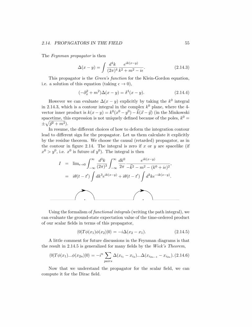
lead to different sign for the propagator. Let us them calculate it explicitlyby the residue theorem. We choose the causal (retarded) propagator, as inthe contour in figure 2.14. The integral is zero if x or y are spacelike (ifx0 > y0, i.e. x0 is future of y0). The integral is then
I = limε→0
∫ ∞−∞
d3k
(2π)3
∫ ∞−∞
dk0
2π
eik(x−y)
−~k2 −m2 − (k0 + iε)2,
= iθ(t− t′)∫dk3eik(x−y) + iθ(t− t′)
∫d3ke−ik(x−y).
Using the formalism of functional integrals (writing the path integral), wecan evaluate the ground-state expectation value of the time-ordered productof our scalar fields in terms of this propagator,
〈0|Tφ(x1)φ(x2)|0〉 = −i∆(x2 − x1). (2.14.5)
A little comment for future discussions in the Feynman diagrams is thatthe result in 2.14.5 is generalized for many fields by the Wick’s Theorem,
〈0|Tφ(x1)...φ(x2n)|0〉 = −in∑pairs
∆(xi1 − xi2)...∆(xi2n−1 − xi2n). (2.14.6)
Now that we understand the propagator for the scalar field, we cancompute it for the Dirac field.

56 CHAPTER 2. FIELDS WITH SPIN
Free Fermion Propagator
We are going to consider the free Dirac field,
ψ(x) =∑s=1,2
∫d3p[bs(p)us(p)e
ipx + d†s(p)vse−ipx
], (2.14.7)
ψ(y) =∑s=1,2
∫d3p′
[bs′(p
′)us′(p′)eip
′y + d†s′(p′)vs′e
−ip′y], (2.14.8)
where we sum on the spin polarization. The annihilation operators are givenby
bs(p)|0〉 = ds(p)|0〉 = 0, (2.14.9)
and the anticommutation relations are
bs(p), b†s′(p′) = (2π)3δ2(p− p′)2ωδss′ , (2.14.10)
ds(p), d†s′(p′) = (2π)3δ2(p− p′)2ωδss′ , (2.14.11)
with zero to all other combinations.Now we want to compute the Feynman propagator
S(x− y)αβ = θ(x0 − y0)〈0|ψα(x)ψβ(y)|0〉, (2.14.12)
= i〈0|Tψα(x)ψβ(y)|0〉, (2.14.13)
where θ(t) is the step function and T is the time-ordered product,
Tψα(x)ψβ(y) = θ(x0 − y0)ψα(x)ψβ(y)− θ(y0 − x0)ψβ(y)ψα(x).(2.14.14)
The minus sign in the last result comes from the anticommutation pro-priety, ψα(x), ψβ(y) = 0 when x0 6= y0, and we will discuss the causalityin the end. To derive the propagator and show that it obeys causality, letus now insert 2.14.8 into 2.14.14,
〈0|ψα(x)ψβ(y)|0〉 =∑s,s′
∫d3pd3p′eipx−ip
′yus(p)αus′(p′)β〈0|bs(p)b†s′(p
′)|0〉,
=∑s,s′
∫d3pd3p′eipx−ip
′yus(p)αus′(p′)(2π)3δ3(p− p′)2ωδss′
=∑s,s′
∫d3peip(x−y)us(p)αus′(p
′)β.

2.14. PROPAGATORS IN THE FIELD 57
Using the result of the sum of all spin polarizations,∑s
us(p)us(p) = −6p+m, (2.14.15)∑s
vs(p)vs(p) = −6p−m, (2.14.16)
we finally have
〈0|ψα(x)ψβ(y)|0〉 =
∫d3peip(x−y)(−6p+m)αβ.
In the same fashion,
〈0|ψα(x)ψβ(y)|0〉 =∑s,s′
∫d3pd3p′e−ipx+ip′yvs(p)αvs′(p
′)β〈0|ds(p)d†s′(p′)|0〉,
=∑s,s′
∫d3pd3p′e−ipx+ip′yvs(p)αvs′(p
′)(2π)3δ3(p− p′)2ωδss′ ,
=∑s,s′
∫d3pe−ip(x−y)vs(p)αvs′(p
′)β,
=
∫d3pe−ip(x−y)(−6p−m)αβ.
These two results can be combined in the time-ordered product, and weget
〈0|Tψα(x)ψβ(y)|0〉 = −i∫
d4p
(2π)4ei(p(x−y) (−6p+m)αβ
p2 +m2 − iε= iS(x− y)αβ,
recovering the Feynman propagator. This is of course the inverse of theDirac operator
(−i 6∂ +m)S(x− y) = δ4(x− y).
Again, let us consider the vacuum expectation value of a time-orderedproduct of more than two fields. We must have an equal number of ψ andψ to get a nonzero result. Concerning the statistics, there is an extra minussign if the ordering of the fields in their pairs is odd permutation of theoriginal ordering. For instance,
〈0|Tψα(x)ψβ(y)ψγ(z)ψδ(w)|0〉 = −i2[S(x− y)αβS(z − w)γδ
−S(x− w)αδS(z − y)γβ
],
58 CHAPTER 2. FIELDS WITH SPIN
Let us analyze these results. We recognize the right side integral of ourderivations to be the commutator of two scalar fields ∆KG(x−y), hence theanticommutator of the Dirac theory is
i∆αβ(x− y) = (−i 6∂ +m)i∆KG(x− y),
and it will vanishes since ∆KG(x − y) vanishes at spacelike separations,concluding that Dirac theory is causal.
From reference [PS1995], we see that if we had quantized the Dirac theorywith commutators instead of anticommutators, we would have a violationof causality, with the exponentials of 2.14.8 summing up instead of having aminus sign and we would have a decaying at equal time and long distances(∆→ emx
x2,mx→∞). In another words, if the theory were to be quantized
with commutators, the field operators would not commute at equal time atdistances shorter than the Compton wavelength, violating the causality.
We had just obtained the Spin-Statistic Theorem, , which states thatfields with half-integer (integer) spin must be quantized as fermions (bosons),making use of anticommutators (commutators). If the theory is quantizedwith the wrong spin-statistic connection, it either becomes non-local (nocausality) or it has no ground state (spectrum with negative norm).

Chapter 3
Non-Abelian Field Theories
Let us generalize the concept of local phase invariance to the Lagrangiandensities with N identical spinor fields that posse global symmetry U(N),
ψ′i(x) = Uijψj(x).
If U → U(x), the Dirac Lagrangian is no longer invariant. For N = 1,it is possible to recover the QED case, (2.8.4), however,, for N > 1, thechanges on the Lagrangian are only canceled if one introduces nonabeliangauge fields, also known as Yang-Mills fields, (Aµ)ij .
Starting with Lagrangians with global spin U(N) = U(1)× SU(N), onehas a set of N Dirac fields ψi, with mass mψ and N scalars fields φi withmass mφ. The gauge fields are N ×N matrices,
(Aµ)ij =
N2−1∑a=1
(Ta)ijAµa(x)ψ, (3.0.1)
where Ta are the generators of SU(N) in the N × N (fundamental) rep-resentation. For this expression to be consistent, Aµ should be an elementof the Lie algebra, where the number of gauge fields is the dimension of thegroup. The normalization is chosen to be
tr (TaTb) =1
2δab.
The covariant derivative is
(Dµ[A])ij = δij∂µ + ig(Aµ)ij , (3.0.2)
D = (6∂ + iε 6A). (3.0.3)
59

60 CHAPTER 3. NON-ABELIAN FIELD THEORIES
The field strength (also a matrix) is
Fµν = δµAν − ∂νAµ + ig[Aµ, Aν ],
=N2−1∑a
Fµν,aTa.
The Yang-Mills Lagrangian is
LYM = ψi[iDµ(A)]ijγµ −mδijψj , (3.0.4)
where the covariant derivative was defined in (3.0.3). One can make globalinvariance (phase U(1) and global SU(N)) by local combining it to thevector fields gauge theories. A resume of the simplest Yang-Mill’s theoryfactors can be seen in the table 3.1.
COMPONENT YANG-MILLS
Fields Dirac ψi, Scalar φiGenerators Ta, a = 1, ..., n2 − 1
Commutator [Ta, Tb] = ifabcTc
Matrix to the Fields Aµ(x)ij =∑n2−1
a=1 Aaµa(x)(TRa )ijCovariant Derivative Dµ[A]ij = δij∂
µ + igAµ(x)ijField Strength Fµν = ∂µAν − ∂νAµ + ig[Aµ, Aν ]
Fields in components Fµν =∑n2−1
a=1 Fµν,aTRa
Table 3.1: The Yang-Mills theory.
3.1 Gauge Transformations
The infinitesimal gauge transformations of the vectors Aµ are given by
UR(x) = eig∑N2−1a−1 Λa(x)TRa ,
= 1 + igN2−1∑a=1
δΛa(x)Ta,
= [1 + igδΛ(x)]ij .

3.2. LIE ALGEBRAS 61
The Aµ transformations are constructed in a way to give the form in-variant Lagrangian,
Finite → A′µ = UAµU−1 +i
g(∂µU)U−1
Infinitesimal → A′µ = Aµ − ∂µδΛ(x) + ig[δλ(x), Aµ(x)],
where the first two terms are the same as in any theory with U(1) gaugeinvariance and the last term is new for non-abelian theories. To complete theLagrangian (3.0.4), we need to supply a new term which is a generalizationof the Maxwell field density, this field strength transforms covariantly as
F ′µν(x) = U(x)FµνU−1,
with the following components, where the last term is Yang-Mills field,
Fµν = U(x)Fµν,ata,
F ′µν,a = ∂µAµ,a − ∂νAµ,a − gCabcAµ,cAν,c,
The gauge invariant Lagrangian is then
LYM = −1
4
∑a
Fµν,aFµνa ,
=1
2tr[FµνF
µν ].
Putting all this together, the Lagrangian invariance under SU(N) forthe spinor is and a scalar is
LSU(N) = |Dµ(A)ijφk|2 −m2φ|φ|2 + ψi(i6D[A]ij −mφδij)ψj −
1
2Tr [Fµν , F
µν ].
3.2 Lie Algebras
In compact Lie Algebras, that are the interest here, the number of generatorsT a is finite. Any infinitesimal group elementg can be written as
g(α) = 1 + iαaT a +O(α2),

62 CHAPTER 3. NON-ABELIAN FIELD THEORIES
where
[T a, T b] = ifabcT c (3.2.1)
are the non-abelian generators commutation relation. If one of the genera-tors commutes with all of the others, it generates an independent continuousabelian group ψ → eiαψ, called U(1). If the algebra contains such commut-ing elements, it is a semi-simple algebra. Finally, if the algebra cannot bedivided into two mutually commuting sets, it is simple. The condition thata Lie Algebra is compact and simple restricts it to four infinity families and5 exceptions.
Unitary Transformations of N-dimensional vectors For η, ξ n-vectors,with linear transformations ηa → Uabηb and ξa → Uabξb, this subgrouppreserves the unitary of these transformations, i.e. it preserves η∗aξa.The pure phase transformation ξae
iαξa is removed to form SU(N),consisting of all N ×N unitary transformations satisfying det(U) = 1.The N2− 1 generators of the group are the N ×N matrices T a underthe condition tr[T a] = 0.
Orthogonal Transformations of N-dimensional vectors The subgroupof unitary N ×N transformations that preserves the symmetric innerproduct: ηaEabξb with Eab = δab, which is the usual vector product,so this is the rotation group in N dimensions, SO(N), or the rotationgroup in 2n+ 1 dimensions, SU(2n+ 1). There is an independent ro-tation to each plane in N dimensions, thus the number of generatorsare N(N−1)
2 .
Symplectic Transformations of N-dimensional vectors The subgroupof unitary N ×N transformations. For N even, it preserves the anti-symmetric inner product ηaEabξb,
Eab =
(0 1−1 0
),
where the elements of the matrix are N2 ×
N2 blocks, Sl(N), with N(N+1
2 .
Representations
If the Lie algebra is semi-simple, the matrices tar are traceless and the traceof two generator matrices are positive definite given by
tr [T ar , Tbr ] = Dab.

3.2. LIE ALGEBRAS 63
Choosing a basis for T a which has Dab ∝ I for one representation meansthat it will be true for all representations:
tr [T ar , Tbr ] = C(r)δab. (3.2.2)
From the commutation relations, one can write the totally anti-symmetricstructure constant as
fabc = − i
C(r)tr [tar , t
br]t
cr. (3.2.3)
For each irrep r of G, there will be a conjugate r given by
tar = −(tar)∗ = −(tar)
T , (3.2.4)
if r ∼ r then tar = UtarU† and the representation is real. The two most
important irreducible representations are the fundamental and the adjoint,which dimensions are given by table 3.2.
Fundamental In SU(N), the basic irrep is the N -dimensional complexvector, and for N > 2, this irrep is complex. In SO(N) it is real andin Sl(N) it is pseudo-real.
Adjoint This is the representation of the generators, r = G, and therepresentation’s matrices are given by the structure constants (tbc)ab =ifabc where ([tbG, t
ca])ae = if bcd(tdG)ae. Since the structure constants are
real and anti-symmetric, this irrep is always real.
FUNDAMENTAL ADJOINT EXAMPLES
SU(N) N , complex N2 − 1 N=4, 4 and 15
SO(N) N , real N(N−1)2 N=4, 4 and 6
Sl(N) N , pseudo-real N(N+1)2 N=4, 4 and 10
Table 3.2: Dimensions of the most important irreps of the compact andsimple Lie algebras.
A good way of seeing the direct application of this theory on fields is,for example, the covariant derivative acting on a field in the adjoint repre-sentation,
(Dµφ)a = ∂µφa − igAaµ(tbG)acφc,
= ∂µφa + gfabcAbµφc,

64 CHAPTER 3. NON-ABELIAN FIELD THEORIES
and the vector field transformation
Aaµ → Aaµ +1
g(Dµα)a.
Casimir Operator
For any simple Lie algebra, the operator T 2 = T aT a commutes with allgroups of generators:
[T b, T aT a] = (if bacT a + T a(if bacT c),
= if bacT c, T a,= 0.
For the adjoint representation,
facdf bcd = C2(G)gab,
d(r)C2(r) = d(G)C(r),
where, for example, for SU(2), C(r) = 12 . ForSU(N), one has the quadratic
Casimir operator coefficient,
C2(r) =1
2
(N2 − 1)
N
3.3 Spontaneous Symmetry Breaking
So far the locally invariant Lagrangian involved only massless vector matri-ces. The spontaneous symmetry breaking makes it possible to the Lagrangianto acquire at once both local gauge invariance and massive vectors. The sys-tem chooses a ground state, with a definitive but arbitrary direction, anychoice breaks the symmetry. While the ground states breaks the symmetry,the Lagrangian remains gauge invariant.
Example: The SU(2)× U(1) Model
In the Higgs mechanism, we postulate a scalar field with a internal symmetryU(1) or great, coupled to a gauge field. We choose a doublet of complexscalar fields φi, i = 1, 2 and write the Lagrangian as
LU(1) = (iDµ(A)φ∗)(iDµ(A)φ)− V (|φ|)− 1
4F 2,
Dµ = ∂µ + igAµ,
Fµν = ∂µAν − ∂νAµ,

3.3. SPONTANEOUS SYMMETRY BREAKING 65
Next step is to write explicitly the
V (|φ|) = −µ2|φ|2 + λ(|φ|2)2,
which has its minimum in |φ0|2 = ν2
2 = µ2
2λ , as in figure (3.1) and (3.2).
Figure 3.1: The Higgs Potential for a real field.
Figure 3.2: The Higgs Potential for a Complex field, in this case the mini-mum is the circle on |φ0|.
The vacuum expectation value, 〈0|φ|0〉, is now different of zero and it isnot unique. Reparameterizing the scalar field to
φ(x) = eiξ(x)2V
V + η(x)√2
, (3.3.1)
where V = µ√λ
, one performs the following replacement of the real and
imaginary parts of φi: Reφ, Imφ → ξ(x), η(x) (phase and modulus). The

66 CHAPTER 3. NON-ABELIAN FIELD THEORIES
potential is then independent of ξ(x) and one has only to replace |φ| by(3.3.1) in V . The mass will be generated to η(x) while ξ(x) will be massless,being only a physical degree of freedom.
V (|φ|2) = −µ2
(V + η(x)√
2
)2
+ λ
(V + η(x)√
2
)4
,
= −µ2
4λ+ µ2η2(x) +
√λµη3(x) +
λ
4η4(x),
where the first term is constant and the third is the interaction. The fieldsξ(x) parametrize the position of φ around the 3-dimensional minimum whileη(x) measures the distance from this minimum. The transference of thephase degree of freedom from φ to Aµ makes it appears as a mass, as it canbe seen at table (3.3)
Start with Degree of Freedom End Degree of Freedom
φ 2 η(x) 1Aµm=0 1 Aµm 6=0 3
V (|φ|) Gauge Invariant V (η) Gauge Invariant
Table 3.3: Degree of freedom for spontaneous symmetry breaking of fields.
The Lagrangian now has a mass term for the field, which is Proca-typemass. Spontaneous symmetry breaking of any kind implies the existence ofa massless scalar, the Goldstone boson. The difference to the Higgs is thethis would be a boson absorbed as a gauge field, i.e. vector.
The theory in terms of new fields is simplified by canceling the nonabelianphase by a SU(2) gauge transformation, which is the Standard Model ofelementary particles is the electroweak group representation, with the gaugebosons W−,W+, Z0. This group transformation takes place by
φ′ = Uφ,
B′µ = UBµU−1 +
i
g(∂U)U−1,
U(x) = e−iξ(x) σ2v .
Now the Lagrangian is independent of the fields ξ and its scalar part is
LHiggs = |iD(B,C)ijφj |2 − V (|φ|2, (3.3.2)
where |φ|2 = |φ†|2 + |φ0|2, (3.3.3)

3.3. SPONTANEOUS SYMMETRY BREAKING 67
The potential and its extremal is
V (|φ|) = −µ2|φ|2 + λ|φ|4,dV
d|φ|
∣∣∣∣∣φ=0
= −2µ2V + 4λV 3 = 0,
Vmin =µ2
2λ.
We write the four degree of freedom of φ as
φ(x) = e−ξ(x)σ2
(0
V+η(x)√2
),
where the three ξ are three massive vectors and one η fields remains distancesfrom Vmin. The Lagrangian, ((3.3.3), is then
LHiggs =1
2[(∂µη)2−2µ2η2]−V λη3+
λ
4η4+
V 2
8[g2(B2
1+B22)+(g′C−gB3)2](V+η)2,
where the V 2 terms give the Proca mass:V 2g2B2
1,2
8 , V2(g′C−gB3)2
8 . The phys-ical particles are then represented by
W± =1√2
(B1 ± iB2),
Z = −( sin θW +B3 cos θW ),
γ = ( cos θW +B3 sin θW ),
where sin θW =g′√g2 + g′
.
The masses of the electroweak gauge bosons are then MW = V g2 ,Mz =
MWcosθw
.

68 CHAPTER 3. NON-ABELIAN FIELD THEORIES

Chapter 4
Quantum Electrodynamics
In this section we are going to understand and to derive the Lagrangianfor the theory of interaction of photons and matter the quantum electrody-namic, represented by (2.8.4). This theory is given by a vector field
Aµ(x) = Cµ cos θw +Bµ3 sin θw.
After the spontaneous symmetry breaking, the photon Lagrangian isMaxwell-form,
LA = −1
4F 2µν(A)− λ
2(∂A)2.
This couples to fermions as
Lferm(ψF , A) =∑
ψF (i(6∂ − ieQF 6A)−mF )ψF ,
where QF is the charge of the fermion in units of positron charge (QF =1, 2
3 ,−13 , 0). The LQED is then LA + Lferm.
Because the minimum coupling, the term ψAψ is not free. As a scalartheory, it makes it necessary to find the Green’s function 〈0|T (ψ(x), ψ(y)Aµ(z), ...)|0〉to derive the S-matrix,
LQED → Z[Jµ(x), kα(y), kβ(z)]→ S-matrix.
By analogy to the scalars fields, one can write the generating functionalfor the Green’s functions,
ZQED[Jµ, kα, kβ] =W [J, k, k]
W [0, 0, 0], (4.0.1)
69
70 CHAPTER 4. QUANTUM ELECTRODYNAMICS
where W are the path integrals and J is the source. The path integral shouldbe over classical c-numbers for fields.
WQED[A, k, k] =
∫[dAµ][dψα][dψβ]ei
∫d4xLQED−i(J,A)−i(k,A)−i(ψ,k),
=
∫[dAµ]W [A, k, k]ei
∫d4x[L(A)−λ
2(∂A)2],
=
∫[dψ][dψ]ei
∫d4xψ[i 6D(A)−m]ψe−i(ψ,k)−i(k,ψ),
where the last two exponentials are the fermion Gaussian integral. We recallthe Gaussian scalar form,
ω(ji) =
∫ ∞−∞
n∏i−1
dxie− 1
2xiMijxJ−Jkxk ,
=
∏n/2
√det M
e−12Jk(M−1)klJl .
The Green’s function is then
G(yi, xi) = 〈0|T [
n∏i=1
ψai(yi)ψbi(xi)]|0〉,
=
n∏i=1
[i δ
δ(kai, yi)][−ikbi(xi)]Z[k, k, A]|k=k=0,
which gives propagator for fermions
SF (z) =1
(2π)4
∫d4ke−ikz
1
6k −m+ iε,
=1
(2π)4
∫d4ke−ikz
6k −mk2 −m2 + iε
,
with 6k 6k = k2. The charged scalar is
Wψ[L, L] =
∫[dφ][dφ∗]e−iSkg−i(L,φ)−i(φ∗,L),
= W [0, 0]e−i∫WZ L
∗(ω)∆(ω−z)L(z),
giving, finally, the generating functional for fermions
Wφ[A, k, k] =
∫DψDψei
∫d4yψ(i 6D(A)−m)ψ−ikψ−iψk,
Z =1
W [0, 0, 0]
∫DψDψDAei
∫d4yψ(i 6D−m)ψ−kψ−ψk−yA.

4.1. FUNCTIONAL QUANTIZATION OF SPINORS FIELDS 71
4.1 Functional Quantization of Spinors Fields
The Grassmann variables defined at section (2.10) are now used in the fieldsψ, defined as a function of spacetime whose values are anticommuting num-ber. We define this field in terms of orthonormal basis functions,
ψ(x) =∑i
ψiφi(x),
where ψ is the Grassmannian variable and φ is the four-component spinor.The Dirac two point correlation function is
〈|Tψ(xi)ψ(x2)|0〉 =
∫DψDψei
∫d4xψ(iγµ−m)ψ]ψ(x1)ψ(x2)∫
DψDψei∫d4xψ(iγµ−m)ψ
(4.1.1)
Using the Gaussian integrals
(∏i
∫dθ∗i dθi)e
−θ∗iBijθj =∏i
bi
= det B,
if θ were an ordinary number, one would have (qπ)n
detB . Also
(∏i
∫dθ∗i dθi)θkθ
4l e−θ∗iBijθj = det B(B−1)kl.
One can then calculate (4.1.1), where the denominator is det(iγµ∂ −m)and numerator is det(iγµ∂−m) −1
iγµ∂−m . From this is possible to recover thepropagator for fermions,
〈0|Tψ(x1)ψ(x2)|0〉 = SF (x1 − x2) =
∫d4k
(2π)4
ie−ik(xi−x2)
6k −m+ iε
4.2 Path Integral for QED
The QED Lagrangian with sources is
LQED =∑
flavors
ψ(i 6D[A]−m)ψ − 1
4F 2(A)− λ
2(∂A)2.
Writing it considering only connected diagrams, i.e all lines connectedto some external point in the Green’s function, we get
Zfree[Jµ, kα, kα] =W [J, k, k]
W [0, 0, 0],
= e−∫w,z [ 1
2Jµ(w)Gµν(w−z)Jν(z)+kα(w)Sαβ(w−z)kβ(z)],

72 CHAPTER 4. QUANTUM ELECTRODYNAMICS
where
W [J, k, k] = Wfreee−
∫d4y[−δk(y)]α(γµ)αβ [iδJµ(y)][iδk(y)].
The greens functions are the variations of J, k, k, and one sets all themequal to zero.
4.3 Feynman Rules for QED
In the same fashion as section 1.10, we can summarize the last results inrules for fermions in an external gauge field. As for charged scalar fields,fermions lines carries arrows, pointing from ψ to ψ. The Feynman rules forQED are:
• Distinguishable diagrams with continuous fermions lines.
• For every fermion line, starting at z pointing to w, one adds i(SF (w−z))αβ, which is i(2π)−4
∫d4k[(k −m)−1]ba.
• For every vector lines, iGµνF (w − z).
• For every vertex −ie(γµ)λσ, as a result of −ieQfδff ′γµdc(2π)4δ4(∑
i pi),where pi labels the momenta of lines flowing.
• For each internal photon line, one adds the factor 12π
∫d4k 1
k2−iε [−gµν+
(1− 1λ)k
µkν
k2i ε].
• Sign rule: (-1) for every fermion loop and (-1) when exchanging pairingof external ψ, ψ.
In the momentum space, the rules are the similar with a few exceptions,
• For every fermion line, starting at z pointing to w, one adds∫
d4k(2π)4
i(6k +m)k2−m2−iε .
• For every vector lines,∫
d4k(2π)4
ik+iε
(− gµν + (1− 1
λkµkν
k2+iε))
.
• For every vertex −ie(2π)4δ4(∑
i ki)(γµ)βα.
4.4. REDUCTION 73
4.4 Reduction
The use the results of the Green’s functions to to find the S-matrix, we needthe residues of single-particle pole defined by∫
d4xeipx〈0|T (ψ(x)ψ(0))|0〉.
The reduction for e+e− → e+e− in terms of the T-matrix is given byS = 1 + iT , where
iT(
(p′, λ′)−, (q′, σ′)+out; (p, λ), (q, γ)in
)=( uα(p′, λ′)
(Rψ(2π)3)12
)( −vβ(q, σ)
(Rψ(2π)3)12
)×Gα′β′,αβ(p′, q′, p, q)trun ×
( uα(p, λ)
(Rψ(2π)3)12
)( −vβ(q′, σ′)
(Rψ(2π)3)12
)∣∣∣∣∣p2=p′2=q2=q′2=m2
The two first parenthesis are the outgoing and incoming fermions andthe two last the incoming and outgoing fermions, respectively.
For vectors, the rules are the same, to get the S-matrix: we go to themomentum space, truncate it and multiply it by, εµ(k)
(RA(2π)3)12
, the incoming
vector, εµ(k′)∗
(RA(2π)3)12
, the outgoing vector.
4.5 Compton Scattering
γe− → γe−.
The S-matrix for the Compton Scattering is
ε′ν(l′) ∗ uβ(p′, σ′)Gtrunεµ(l) · uα(p′, σ).
1
RARψ(2π)6.
4.6 The Bhabha Scattering
The Bhabha scattering is an example of tree level gauge theory cross section.
e+e− → e+e−.
The S-matrix level is gauge invariant (independent of gauge theory fixing),
iM(p4, σ4, p3, σ3, p2, σ2, p1, σ1) =

74 CHAPTER 4. QUANTUM ELECTRODYNAMICS
Figure 4.1: The two tree Feynman diagrams of the Bhabha Scattering. Inthe internal line, µ and ν couple together by the propagator of the photon.The first diagram is the scattering exchange and the second the annihilationfollowed by a pair creation, All momentum are on-shell.
There are two diagrams (figure 4.1),
iM = (2π)4δ4( 4∑i=1
kµi
)×[( i
−k2 −m[−ieγµ]
i
k4 −m
)bd−
− i
|k2 + k4|2
(− gµν + (1− 1
λ)
1
|k2 + k4|2
)×( i
−k3 −m[−ieγµ]
i
k1 −m
)ca
− other diagrams where k2 ↔ k3, b↔ c.
The Green’s function is always pure imaginary for tree diagrams and Tand M are always real. From the result of the reduction,
T = σ4(∑
ki
) 1
(2π)6M,

4.6. THE BHABHA SCATTERING 75
where we only need to find M. From the diagrams,
iM(pi, σi) = v(p2, σ2)(−ieγ)µv(p4, σ4)×1
(p2 − p4)2
(− gµν + (1− 1
λ)(p2 − p4)µ(p2 − p4)ν
(p2 − p4)2
)×
u(p2, σ2)(−ieγ)µ)u(p1, σ1)−−v(p2, σ2)(−ieγ)µ)v(p1, σ1)×
1
(p2 − p1)2
(− gµν + (1− 1
λ)(p2 − p1)µ(p2 − p1)ν
(p2 − p1)2
)×
u(p3, σ3)(−ieγµ)u(p4, σ4)],
which still depends on the gauge fixing parameter λ. The Green’s functionalso depend on the gauge while the physical amplitudes does not. Theterms multiplied by λ are dropped and one needs to keep −gµν
k2for photon
propagation. Simplifying (4.1), the first diagram is
= v2(−eγµ)u1
(−igµν
(p1 + p2)2
)u3(−eγµ)v4.
The second is
= −v2(−eγµ)v4
(−igµν
(p1 + p4)2
)u3(−eγµ)u1.
Hence, one has
M = v2(−ieγ)µv4
( 1
(p2 − p4)2
)u3(−ieγ)µu1 −
v2(−ieγ)µu1
( 1
(p1 − p3)2
)u3(−ieγ)µv4.
The gauge invariance of the general result for the S-matrix is common toall orders in QED and the other gauges theories. In general,M can dependson all invariants pipj , piσj , σjσk, they are all Lorentz invariant number. How-ever, certain dependences are not allowed by parity of QED. For example,let us suppose we have
M∝ A(p1, p2) + σipjB(pi, pj).
In the frame σ0 = 0 this changes the spin under xp− x. In transformedfields where x = −x,M = A−σipjB, not allowed in QED, however allowedin the weak interactions.
The Feynman identity (a generalization of the Ward identity) is
u(p2)(6p2 − p1)u(p1) = 0.

76 CHAPTER 4. QUANTUM ELECTRODYNAMICS
4.7 Cross Section
For a fixed spin, the relations for M are the same as for scalars. We cannow compute the cross section for fermion+antifermion scattering,
dσ
dt=
1
16πs(s− 4m2)|M(pi, σi)|2,
where t = (p3 − p1)2 = (p4 − p2)2, s = (p1 + p2)2, u = (p4 − p1)2.
4.8 Dependence on the Spin
Most experiment involves non-polarized beams at the target, i.e. incoherentcombination of spins. For unpolarized σ’s, we average over initial state spinand then sum over the final state,
• First we look to the general initial state: |Ain〉 =∑N
i=1CAi |σi〉,
where N is the number of different spin states, for example, for twoparticles with spin-half, N = 4.
• If we have a unpolarized beam for a particle process A→ B, then
|MA→B|2 ∝ |〈Bout|Ain〉|2,
=
N∑u,j=1
C∗jCi〈σj |Bout〉〈Bout|σi〉.
• If there is no polarization, we average the C’s: 〈Ci|C∗j 〉 = 1N δij , and
one has 〈|MA→B|2〉 = 1N
∑i |〈Bout|σi〉|2, which is the average over the
initial states.
• For the final states, just sum over B’s definitive spin. Applying toBhabha scattering, we then see the simplification in the unpolarizedcase (it is not necessary to compute M for the fixed spin).
• Rather than calculate v2γ∗v1, etc, we use the complex conjugate of the
identity γ0γµγ = (γµ)†. Hence, any factor (ui, γα1, γα2, ...γαn, uj)∗ =
ujγ2nγ2n−1...γ1ui. This will generate four therms in the Bhabha scat-tering, which are the four cut diagrams, related to the optical theorem.

4.8. DEPENDENCE ON THE SPIN 77
Calculating for the first cut diagram, we have
e4
s2
∑s
(v2γµu1)(u1γ
νv2)(u3γ5v4)(v4γµu3).
Using the projection relations,
∑s
(ui)β(ui)α =∑λ
uβ(piλ)uα(piλ) = (6p1 +m)αβ,∑s
(vi)β(vi)α =∑λ
vβ(pk, λ)vλ(pj , λ) = (6p2 +m)αβ,
finally giving
e4
s2
∑s
Tr dirac[(6p1 +m)γν( 6p2 +m)γa]. Tr dirac[(6p3 +m)γµ(6p4 +m)γnu]
.
The following other three diagrams have: (b)-2 traces and (c), (d)-onetrace. For the second of the cut diagrams, we have
e4
s2
∑s
uβ(p3, λ3)(γµ)βγuγ(p1, λ)uλ(p1, λ1)(λτ )γτuτ (p3, λ3),
and the only trace is given by the piece in the middle,
uλ(p1, λ)uλ(p1, λ1) = ( 6p1 +m)λσ.
It is straightforward to find the other two cut diagrams.

78 CHAPTER 4. QUANTUM ELECTRODYNAMICS
4.9 Diracology and Evaluation of the Trace
To calculate the traces of the diagrams in the Feynman, we define usefulproprieties of the Dirac matrices,
tr 6a 6b = 2ab,
tr γµ = 0,
tr (odd numbers of γ) = 0,
tr [γ5 6a 6b6c6d] = 4iεµνλνaµbνcλdσ,
tr [ 6a 6b6c6d] = 4(abcd+ adbc− acbd),
tr [∑i
6ai] =
n−1∑i=1
ana(i − 1)i−1 Tr
γ5 = iγ0γ1γ2γ3,
(γ5)2 = 1,
(γ0)† = γ0,
(γµ)† = γ0γµγ0,
γ5, γµ = 0,
6a6b = ab− 2iaµSµνbν ,
Sµν =i
4[γµ, γν ],
γµ 6aγµ = −2 6a,γµ 6a 6bγµ = 4ab,
γµ 6a 6b6cγµ = −γµ 6a 6bγµ 6c+ 2 6c6a6b,= −s 6c6a, 6b+ 2 6c6a 6b,= −2 6a6b6c,
6a, 6b = 2ab.

4.9. DIRACOLOGY AND EVALUATION OF THE TRACE 79
Now, we estabilish the follow relations,
tr Mab = Maa ,
tr γµ = 0,
tr γ5 = 0,
tr γµγνγλ = 4gµν ,
tr γµγν = 0,
tr 6a6b = 4gµν ,
tr γ5γµγνγλγσ = 4iεµνλσ,
tr γµγνγλγσ = 4(ηµνηρσηρσ − ηµρηνγ + ηµσηνρ),
tr (6a1 6a2 6a3 6a4) = 4[(a1a2)(a3a4)− (a1a3)(a2a4) + (a1a4)(a2a3)],
tr (6a1 6a2...6an) =n−1∑i=1
(an.ai)(−1)i−1tr ( 6a1 6a2...6an−1).
Finally, we evaluate the traces,
tb1µν = Tr [γν( 6p1 +m)γµ( 6p3 +m)],
= Tr [γν 6p1γµ 6p3] +m2 Tr [γνγµ],
= 4(pν1pµ3 + pν3p
µ1 − g
νµp1p3) + 4m2p1p3.
and
tb2µν = Tr [γν( 6p2 +m)γµ( 6p4 +m)],
= Tr [γν 6p2γµ 6p4] +m2 Tr [γνγµ],
= 4(pν2pµ4 + pν4p
µ2 − g
νµp2p4) + 4m2p2p4.
The full trace results to be a Lorentz invariant,
Tb = tb1µν(tb2)µν
= 16(pν1pµ3 + pν3p
µ1 − g
µνp1p3)(p2νp4µ + p4νp2µ − gµνp2p4)− 2m2(p1p3 + p1p3).
Finally, we are in the very moment we can calculate the cross section,
σ
dt=
2πα2
s(s2 − 4m) 1
s2 [(u− 2m2)2 + (t− 2m2)2 + 4m2s]
+ 1t2
[(u− 2m2)2 + (s− 2m2)2 + 4m2s]
+ 1st [(u− 2m2)2 + 4m2(u− 2m2)] ,

80 CHAPTER 4. QUANTUM ELECTRODYNAMICS
where α = e2
4π and the Mandelstam variables are
s = (p2 + p2)2,
t = (p1 − p3)2 = (p2 − p4)2,
u = (p1 − p4)2 = (p2 − p3)2.
The behavior of the cross section in terms of the center of mass scatter-ing angle is derived from (4.9.1) for the spin average case with equal massparticles. Let θ be the center of mass angle between pi and p3, we rewritethe Mandelstam variables as
s = 4E2,
t = −4(E2 −m2) sin2 θ
2,
u = −4(E2 −m2) cos2 θ
2.
The previous calculation is simplified when we take the limit m → 0,which is the same limit which E and themoment transfered go to zero (fora fixed m). There is no specified spin dependence but the answer dependson the spin of the field.

Chapter 5
Electroweak Theory
The electroweak theory is represented by the Lagrangian
LEW = − g√2
∑charged
[u
(1)1 6W
+l(L)i + li 6W−u(L)
i
]− g
cosθW
∑neutral
[u
(1)1 6Zu
(L)i + l
(L)i 6Z(γ5 + 4sin2θW − 1)
].
It consists of two parts, a charged current and interactions, couplingcharged leptons to neutrinos (only left-handed), and a ]it neutral current,coupling Z boson to neutrinos or charged leptons (left-handed and right-handed). The relevant vertice are
− ig
2√
2[γµ(1− γ5)]βα,
− ig
2cosθW[γµ(1− γ5)]βα,
− ig
4cosθW[γµ(γ5 + (4sin2θN − 1))]βα.
The propagator is( i
6k −m
)αβ
i
q2 −M2
(− gµν +
qµqνM2
).
5.1 The Standard Model
The Standard Model of Particles is represented by three gauge field theories,SU(3)× SU(2)×U(1). The group and fields couplings are described in thetable 5.1.
81

82 CHAPTER 5. ELECTROWEAK THEORY
SU(3) SU(2) U(1)
Gµa , a = 1, ..., 8 Bµb ,b = 1, 2, 3. Cµ
G are gluons B is W± and Z C is γgs g g′
Table 5.1: The Standard Model.
For each Dirac and scalar field, one must still specify how they couple.U(1) Is related to the charge, generates the phase transformation on the
hypercharge Y (eiY2α(x)). SU(2) is related to the electroweak interactions,
giving by the Z,W± bosons.The Lagrangian of the Standard Model is
LSM = Lvectors + Lhiggs + Lquarks + Lleptons,
Lvectors = −1
2TrSU(3)[F
2µν(A)]− 1
2TrSU(2)[F
2µν(B)]− 1
4F 2µν(C).
where the two first terms are bosons and the two last fermions.The general form of the covariant derivative is
Dµ[A,B,C] = ∂µ + igsAµ,aT(R3f )
a + igBµ,bT(R2e)
b + ig′Y
2Cµ.
The Standard Model distinguishes left-handed and right-hand parts ofthe Dirac field, where
ψL =1
2(I ∓ γ5)ψ.
Singlets fields (under SU(3), SU(2), U(1)) have a missing term Dα. Forexample, leptons are singlets under SU(3), and other cases can be seen inthe table 5.2.
R(3)f R
(2)e Y
qkR 3 1,1 4/3, -2/3qkL 3 2 (u and d) 1/3lkR 1 1,1 0,-2lkL 1 2 (νe and e) -1φ 1 2 1
Table 5.2: Summary of the representations of the Standard Model.

5.1. THE STANDARD MODEL 83
Hypercharge Construction
The way we represent the hypercharge in the gauge group formalism is bywriting
QEM =Y
2+ I
SU(2)L3 ,
where I3 is equal to 1/2 for Ul, µl and -1/2 for dl, l. The symmetry SU(2)does not allow a Dirac mass term: mψψ = m(ψLψR + ψRψL), since ψLand ψR transforms differently. These fields gets mass by the same Higgsmechanism of vectors. The Higgs fields are represented as
Φ =
(φ†, I3 = 1
2φ0, I3 = −1
2
).

84 CHAPTER 5. ELECTROWEAK THEORY

Chapter 6
Quantum Chromodynamics
6.1 First Corrections given by QCD
The Lagrangian of QCD is
L = ψi(iγµδµ −m)ψi − g(ψiγ
µT aijψi)Gaµ +
1
4GaµνG
µνa . (6.1.1)
In this section, we will calculate the first corrections due the strong force:the first-order radiation of gluons jets on the process e+e− → gqq, a QCD’sprocess1. This can be seen as an coupling terming of fermions to gluons atthe Lagrangian,
gψfiγµγfiBµ, (6.1.2)
with color indexes i = 1, 2, 3 and f the quark flavors. One can then calculatethe cross section for emission of one gluon. Writing the four-momentum ofthe equation as qµ = q0, ~q, and the momentum of quark, anti-quark andgluon as kµi − (ωi,~k), i = 1,2 and 3, the ratio of the center-of-mass energyof the particle i to the maximum available energy is given by
xi =2kiq
q2=
2Ei√s, (6.1.3)
where∑xi = 2. To write the differential cross section, equation 6.1.4, one
needs to calculate the phase space and matrix |M|2. From 6.1.3 one cancalculate the range of integration, finding 0 ≤ xq, x2 ≤ 1− µ
q .
85

86 CHAPTER 6. QUANTUM CHROMODYNAMICS
dσn =1
q2[1
4
∑spins
|M|2][
∫Πn]. (6.1.4)
Choosing the frame where ~q = 0, one has k1+k2+k3 = 0, the three-bodyphase space is given by∫
Π3 =
∫d3k1d
3k2
(2π)58ω1ω2ω3δ(q0 − ω1 − ω2 − ω3), (6.1.5)
=1
32π3
∫dω1dω2σ(q0 − ω1 − ω2 − ω3), (6.1.6)
=q2
128π3
∫dx1dx2. (6.1.7)
Calculating explicitly the two Feynman diagrams with emission of onegluon, squaringM, finding the two traces, electron (pure QED) and quarks(some extra tricks, see [PS1995]), one has
1
4
∑spins
|M|2 =1
4
(e4g2Q2F
q4
)Tr [6pγµ 6pγα] Tr [ 6pΛβµ 6pΛαβ], (6.1.8)
=e4g2Q2
F
4q4IµαGµα. (6.1.9)
Gathering everything on 6.1.4, one has the differential cross section:
dσ =e4g2Q2
F
4q4
1
256πIµα
∫dx1dx2Gµα, (6.1.10)
=2α2α2
s
3
Q2f
q2
∫8(x2
1 + x22)
(1− x1)(1− x2)dx1dx2. (6.1.11)
d2σ
dx1dx2=
8σ2σ2sQ
2f
3q2
8(x21 + x2
2)
(1− x1)(1− x2). (6.1.12)
Integrating this on the range 0 ≤ x1, x2 ≤ 1 gives an integral that di-verges. One then sets the range of integrations are the infrared divergencesas µ → 0, and integrating with µ 6= 0 one gets the infrared terms propor-tional to ln(µq ), which are related to the infrared cut of QCD. These singu-larities are not physical but the breakdown of perturbation theory, meaningthat the mass of quarks and gluons are never on-shell, as was supposed

6.2. THE GROSS-NEVEU MODEL 87
on these calculations (e.g. ωi cannot be of the same order of the hadronmasses).The 2-3 kinematics collapses to an effective 2-2 due to an emissionof soft gluon or to collinear splitting of a parton on two. There are then twopossible emissions, soft (when ω3√
s→ 0) and collinear (when θi3, (1−xi)→ 0
from (1− xi) =xjω3
q (1− cos θj3)).
6.2 The Gross-Neveu Model
The Gross-Neveu model is a quantum field theory model of massless Diracfermions with one spatial and one time dimension, with an attractive short-range potential, where fermion pairs composite condensates to break Z2-symmetry and acquire mass. It was introduced as a toy model for quantumchromodynamics.The Lagrangian of the model is given by
L = ψii6∂ψi +1
2g2(ψiψi)
2.
This theory is invariant under ψi → γ5ψi and the chiral symmetry forbidsthe appearance of fermions mass.
Proof. ψiψi = ψ†i γ0ψi = ψ†(γ5γ0γ5)ψi = −ψ†γ0ψi = −ψiψi. Therefore we
see that ψiψi = const. Same proof can be made for ψii6∂ψi. This is a Z2
symmetry.
The theory is renormalizable in two dimensions.
Proof. The mass dimension in a theory in D-dimensions is D−12 . The space-
time volume has dimension −D. The Lagrangian density has mass dimen-sion D. Therefore, for D = 2, we have D−1
2 = 12(−ε). Since the four-fermion
operator has dimension=2, g is dimensionless and renormalizable.
6.3 The Parton Model
The intrinsic scheme of the elementary particles in nature is given by theircomposed quarks. We call parton all the quarks and gluons of inside aparticle. We represent the parton distribution in the vacuum sea by
us(x) = us(x) = ds(x) = ds(x) = ss(x) = ss(x) = s(x). (6.3.1)
On another hand, we represent the valence quarks, such as in the proton,
u(x) = uv(x) + us(x), (6.3.2)
d(x) = dv(x) + ds(x). (6.3.3)

88 CHAPTER 6. QUANTUM CHROMODYNAMICS
Summing all the contribution of these partons, it is necessary to recovercharges, baryon number and strangeness,∫ 1
0[u(x)− u(x)]dx = 2, (6.3.4)∫ 1
0[udx)− d(x)]dx = 1, (6.3.5)∫ 1
0[s(x)− s(x)]dx = 0. (6.3.6)
The presence of gluons emissions is signaled by a quark jet and a gluonjet in the final state, either in the direction of the virtual photon (pT 6= 0).
Deep Inelastic Scattering
At a very high resolution (when the transfered momentum q2 is large), thenucleon can be resolved as a collection of almost non-interacting point-likeconstituents, the partons. When the resolution scale λ of the effective probeq is smaller than the typical size of the proton (∼ 1 fm), the internal structureof the proton is probed and we have the deep inelastic regime (DIS), 6.1-a.Defining Q2 = −q2 > 0 as the off-shell momentum of the exchanged photon,the resolution scale is λ = ~
Q .
Figure 6.1: a)DIS, b) Elastic scattering.
The electron-quark scattering, e−(k)+q(pq)→ e−(k′)+q(p′q), is given by
the QED differential cross section (partonic massless limit (s+ t+ u = 0)),where the matrix element squared for the amplitudes are∑
|M|2 = 2e2qe
4 s2 + u2
t2.
In terms of the Mandelstam variables, s = (k + pq)2, t = (k − k′)2, u =
(pq − k′)2. In the frame which the proton is moving very past, P M , we

6.3. THE PARTON MODEL 89
can consider a simple model where the photon scatter a pointlike quark withε fraction of the momentum vector p = ξP . The deep inelastic kinematicsare t = q2, u = s(y − 1), s = ξQ2/xy. The massless differential cross sectionis then
dσ
dt=
1
16πs2
∑|M|2,
where, substituting the kinetic variables,
dσ
dQ2=
2πα2e2q
Q4[1 + (1− y)2].
The mass-shell constraint for the outgoing quark p′2q = 0 suggest thatthe structure function probes the quark with ξ = x. With s the square ofthe the center-of mass energy of the electron-hadron, the invariant s is
s = (p+ k)2 ∼ 2p . k ∼ xs.
Writing∫ 1
0 dxδ(x − ξ) = 1 we have the double cross section for the quarkscattering process,
d2σ
dxdQ2=
4πα2
Q4[1 + (1− y)2]
1
2e2qδ(x− ξ).
The event distribution is in the x − Q2 plane. The parton distributionfunctions (PDFs) parametrizes the structure target as ’seen’ by the virtualphoton and which are not computable from first principles through pertur-bative calculations.
The Bjorken limit is definite as Q2, q →∞, with x fixed. In this limit thestructure functions obey an approximate scaling law, i.e. they only dependon x, not in Q2, as we can see in figure 6.2. Bjorken scaling implies thatthe virtual photon scatters off pointlike constituents, since otherwise thestructure functions would depend on the ratio Q/Q0, some length scale.
Dividing it by (1 + (Q2
xs )2)/Q4, we remove the dependence of the QEDcross section and the result is independent of Q2. The result is that thestructure of the proton scales to an electromagnetic probe no matter howhard it is probed.
We see an anti-screening effect where the coupling constant appearsstrong at small momenta, behaviors called asymptotic freedom and belong-ing to a non-abelian gauge theory. These are the only field theory withasymptotic freedom behavior with interacting vector bosons which couldbind the quarks. This gauge theory confirmed the Bjorken scaling, with theevolution of the coupling very slow, following a logarithmic distribution inmomentum. The scaling violations corresponds to a slow evolution of theparton distributions Fi(x) over a logarithmic scale Q2.
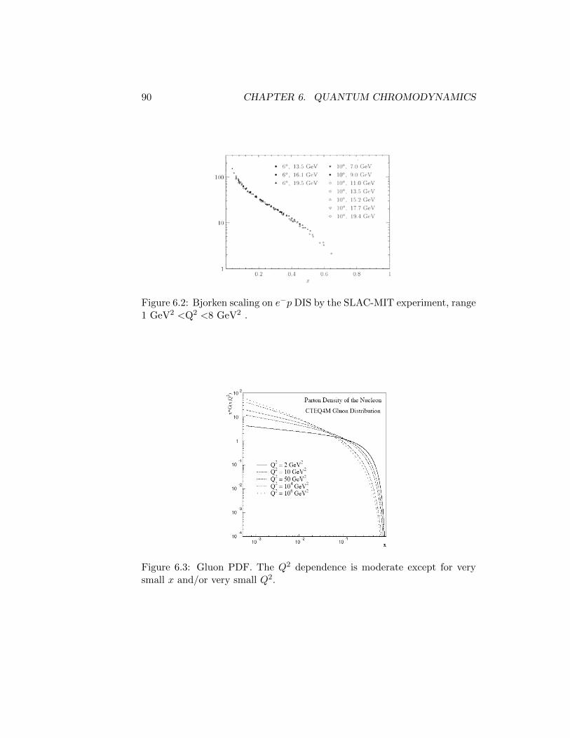
90 CHAPTER 6. QUANTUM CHROMODYNAMICS
Figure 6.2: Bjorken scaling on e−p DIS by the SLAC-MIT experiment, range1 GeV2 <Q2 <8 GeV2 .
Figure 6.3: Gluon PDF. The Q2 dependence is moderate except for verysmall x and/or very small Q2.

6.3. THE PARTON MODEL 91
Figure 6.4: The up PDF from valence and sea. The Q2 dependence is largefor small x and small Q2.
The Running Coupling
In the previous simple parton model, the structure functions scale in theasymptotic (Bjorken) limit Q2 →∞. In QCD, next to the leading order inαs, this scaling is broken by logarithms of Q2. A quark can emit a gluon
and acquire large kT with probability proportional to αsdk2Tk2T
. The integral
extend up the kinetic limit k2T ∼ Q2 and gives contributions proportional to
αsQ2, breaking the scaling.
The screening behaviors on QED is giving by summing the higher ordercorrections in terms of the general form αn[log(Q2/Q2
0)]m and retaining onlythe leading logarithm terms (m = n). Therefore the vacuum polarizationaffects the coupling in QED as
α(Q2) =α(Q2
0)
1− α(Q20)
3π log(Q2
Q0
) ,the leading logarithm approximation.
For QCD, since gluons also emit additional gluons and similar chargesattract themselves, the effect is anti-screening, the effective color chargedecreases as one probes the original quark. Therefore, this phenomena ofasymptotic freedom is given by the QCD running coupling,
αs(Q2) =
αs(µ2)
1 + αs(µ2)12π (11Nc − 2Nf ) log
(Q2
µ2
)where Nc is the number of color charges, Nf the number of quarks flavors
and µ the renormalization scale. To make αs independent of the renormal-

92 CHAPTER 6. QUANTUM CHROMODYNAMICS
ization scheme, we introduce a scale Λ2QCD,
Λ2QCD = µ2e
−12π
(11Nc−2Nf )αs(µ),
which experimentally is ∼ 200. In this QCD scale, the coupling constantcan be written as
αs(Q2) =
12π
(11Nc − 2Nf )log(Q2/Λ2QCD)
,
where we see αs → 0 when Q2 → ∞ and when Q2 Λ2QCD we have hard
interactions.
Figure 6.5: At Q2 increases, it is possible to probe shorter distances. Atlarge Q2, the large x quarks are more likely to loose energy due to gluonradiation.
Leading Log Approximation
Collinear photon emission in QED at high energies is already associatedwith mass singularities and it leads to an analog of parton distribution forelectron. Gribov and Lipatov showed that in a field theory with dimen-sionless coupling α, the DIS structure functions are represented as a sum ofRutherford cross sections og lepton scattering the point-like charges particle,weighted by a parton density Ffi (x).
Logarithmic deviations from the true scaling behavior had been predictedfor the PDFs, reveling the internal structure of PDFs which corrections aregiven by Ffi (x, logQ2). Physically: DIS with a photon with Q2 correspondto the scattering of that virtual photon on a quark of size 1/Q. From QCDbremsstrahlung, we have
dω ∝ α2
∫ Q2dk2⊥
k2⊥,

6.4. THE DGLAP EVOLUTION EQUATIONS 93
therefore the collinear photon emission cost a factor not of α but α log(s/m2), and multiple collinear photons gives contributions of order (α log(s/m2))m.therefore it makes the total probability of extra parton production large,since for α2 1, log Q2 is high enough and ω ∝ α2 log Q2 ∼ 1. In QCD,
the corresponding factor for collinear gluon emission is αs(Q2) log Q2
µ2.
In QED, when k2 → 0, we can write the expansion for gµν in termsof massless polarization vector and when the singular term as the photonmomentum q goes on-shel is given by −ig
µν
q2→ +i
q2∑
i εµTiε
νT i in the calculus of
the amplitudes, decoupling the photon/electron emission vertex. The finalcross section is giving by
σ(e−X → Y ) =
∫ 1
0dz
α
2πlog
s
m2
[1 + (1− z)2
z
]× σ(γY → Y ),
=
∫ 1
0dz Fγ(z)× σ(γX → Y ).
Considering the limit of the divergence z = 0 = 1 − x, the soft partonemission or infrared divergent, we see it is balanced by negative contributionsfrom diagrams with soft virtual photons. Thus, to order α, the partondistribution of electrons has the form
Fγ = δ(1− x) +α
2πlog
s
m2
(1 + x2
1− x−Aδ(1− x)
), (6.3.7)
where the first delta is the zeroth order of the expansion and A we willexplicitly calculate in the following sections.
6.4 The DGLAP Evolution Equations
The hadron evolve with energy Y = log(1/x), and for some values of (Q2, x),although the hadron is no longer perturbative, the evolution still is (exceptfor low Q2). Therefore, we can construct evolution equations in this two thetwo variables of the phase space: log(1/x) and logQ2.
In figure 6.6 we see that when Q2, Y small, the proton is represented bythree valence quarks and the gluon vacuum oscillations is very quickly. In-creasing Q2, the probe resolution, means to decrease the time of interactionand the probes resolves more and more of these fast fluctuations increasesthe number of partons seen. However, the space occupied by them decreases:at each Q2 step the proton becomes more dilute. This evolution is describedin QCD by the DGLAP equations.
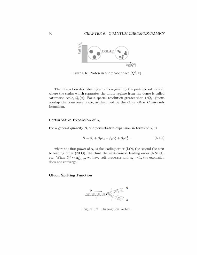
94 CHAPTER 6. QUANTUM CHROMODYNAMICS
Figure 6.6: Proton in the phase space (Q2, x).
The interaction described by small s is given by the partonic saturation,where the scales which separates the dilute regime from the dense is calledsaturation scale, Qs(x). For a spatial resolution greater than 1/Qs, gluonsoverlap the transverse plane, as described by the Color Glass Condensateformalism.
Perturbative Expansion of αs
For a general quantity B, the perturbative expansion in terms of αs is
B = β0 + β1αs + β2α2s + β3α
3s... (6.4.1)
where the first power of αs is the leading order (LO), the second the nextto leading order (NLO), the third the next-to-next leading order (NNLO),etc. When Q2 ∼ Λ2
QCD, we have soft processes and αs → 1, the expansiondoes not converge.
Gluon Spitting Function
Figure 6.7: Three-gluon vertex.

6.4. THE DGLAP EVOLUTION EQUATIONS 95
The element matrix (Feynman rules) for 6.7 is
M = −igfabc[ε∗(q)ε(p)ε∗(k)(p+ q) +
+ ε∗(q)ε∗(k)ε(p)(−q + k)−− ε∗(k)ε(p)ε∗(q)(k + p).
The color factor of the squared average amplitude
1
da
∑b,c
fabcf∗abc = CA = 3,
where CA is the Casimir for the adjoint representation of SU(3) (gluon). Wechoose the gluon (left, right) polarization
εR⊥ =1√2
(−1,−i), εL⊥ =1√2
(1,−i).
The squared amplitude is then
M2 =12g2p2
⊥z(1− z)
z2(1− (1− z)z) + (1− z)2(z + (1− z)2
z(1− z).
In the light-cone basis, the kinematics of a a real gluon can be writtenas
p = (√
2p, 0.0),
q ∼ (√
2zp−√
2p2⊥
4zp,
√2p2⊥
4zp, p⊥, 0),
k ∼ (√
2(1− z)p+
√2p2⊥
4zp,−√
2p2⊥
4zp,−p⊥, 0).
Using these kinematic relations we have
1
4π
∑|M|2 ∝ Pg←g(z)
= 2CA
[ z
1− z+
1− zz
+ z(1− z)
+ Aδ(1− z)]

96 CHAPTER 6. QUANTUM CHROMODYNAMICS
Calculating the Normalization
We know calculate the normalization A from the last equation. We take intoaccount the process where the gluons remains with its identity and normalizethrough defining a distribution that can be integrated by subtracting a deltafunction. We define a function that agrees to 1/(1−z) for all values of x < 1,
1
(1− z)+=
1
(1− z), ∀z ∈ [0, 1[,
the integral of this distribution with any smooth function f(x) gives the newdistribution ∫ 1
0dz
f(z)
(1− z)+=
∫ 1
0dzf(z)− f(1)
1− z.
In the QED process this normalization was A = 23 . For our gluon split-
ting function we are going to use the relation (4.93) of [WEINBERG2005].The leading-order DGLAP splitting function Pa←b(x) has an attractive in-terpretation as the probabilities of finding a parton of type b with a fractionx of the longitudinal momentum and a transverse momentum squared muchless than µ2. The interpretation as probabilities implies the sum rules in theleading order, ∫ 1
0
dx Pq←q(x) = 0, (6.4.2)∫ 1
0
dx x[Pq←q(x) + Pg←q(x)
]= 0, (6.4.3)∫ 1
0
dx x[2NfPq←g(x) + Pg←g(x)
]= 0. (6.4.4)
We will use the last one to find the overall normalization, A, on 6.4.2,substituting the know splitting functions. For the first term,∫ 1
0
dx x[2NfPq←g(x)
]=∫ 1
0
dx x[2Nf Tr [x2 + (1− x)2]
]=
Nf
∫ 1
0
dx x[x2 + (1− x)2
]=Nf
3.

6.4. THE DGLAP EVOLUTION EQUATIONS 97
The second therm (x = 1− z),∫ 1
0
dx x [Pg←g(x)] =
2CA
∫ 1
0
dx x[ x
1− x+
1− xx
+ x(1− x)]
=
6
∫ 1
0
dx x[x− 1
1− x+x− 1
x+ x(1− x)
]=
6(− 11
12
).
Summing up both terms, we find 6A = 112 −
Nf3 . Finally, the leading-
order corrected splitting function, 6.4.2, is then given by
P 0g←g(z) = 6
[ z
1− z+
1− zz
+ z(1− z) +(11
12− Nf
18
)δ(1− z)
)],
.
In the language of the expansion on 6.4.1, the (gluon) splittings functionscan be written as
Pg←g(z, αs) = P 0g←g +
αs2πP 1←gg(z) + ...
Proprieties of Splitting Functions
Pq←q(z) = Pq←q(1− z),Pq←g(z) = Pq←g(1− z),Pg←g(z) = Pg←g(1− z).
Because of the charge conjugation invariance and SU(Nf ) flavor sym-metry,
Pqi←qj (z) = Pqi←qj
Pqi←qj (z) = Pqi←qj
Pqi←g(z) = Pqi←g = Pq←g
Pg←qi(z) = Pg←qi = Pg←q

98 CHAPTER 6. QUANTUM CHROMODYNAMICS
Altarelli-Parisi Equations
Together with the other splitting functions we can write explicitly the Altarelli-Parisi equations which describes the coupled evolution of the PDFs, Fg(x,Q),Ff (x,Q),Ff (x,Q),
for each flavor of quark and antiquarks (treated as massless at Q),
d
dlogQFg(x,Q) =
αs(Q2)
π
∫ 1
x
dz
z
[Pg←q
∑f
(Ff (
x
z,Q) +
Ff (x
z,Q)
)+ Pg←g(z)Fg(
x
z,Q)
],
d
dlogQFf (x,Q) =
αs(Q2)
π
∫ 1
x
dz
z
[Pq←qFf (
x
z,Q) +
Pq←g(z)Fg(x
z,Q)
],
d
dlogQFf (x,Q) =
αs(Q2)
π
∫ 1
x
dz
z
[Pq←qFf (
x
z,Q) +
Pq←g(z)Fg(x
z,Q)
],
Generally, the DGLAP equation is a (2Nf +1)-dimensional matrix equa-tion in the space of quarks, antiquarks and gluons.
6.5 Jets
A constituent cannot acquire a large transverse momentum except through-out exchange of gluon. A process suppressed by the smallness of αs at largemomentum scales. We have then strong gluon radiation in limit of large Q2:if the gluon has large transverse momentum we will see three jets.
The kinematic of decay of a hadron Qq or Qqq is the kinematic of decayof Q. The four momenta is given by
(∑
pi)2 = m2
Q, (6.5.1)
which is difficult to measure because of the missing energy of neutrinos. Aconsequence of a large energy released is that the final particles will have a

6.5. JETS 99
Figure 6.8: Dependence on Q2 of the quark PDF in a DIS electron-proton.The curves are the results from Altarelli-Parisi equations.
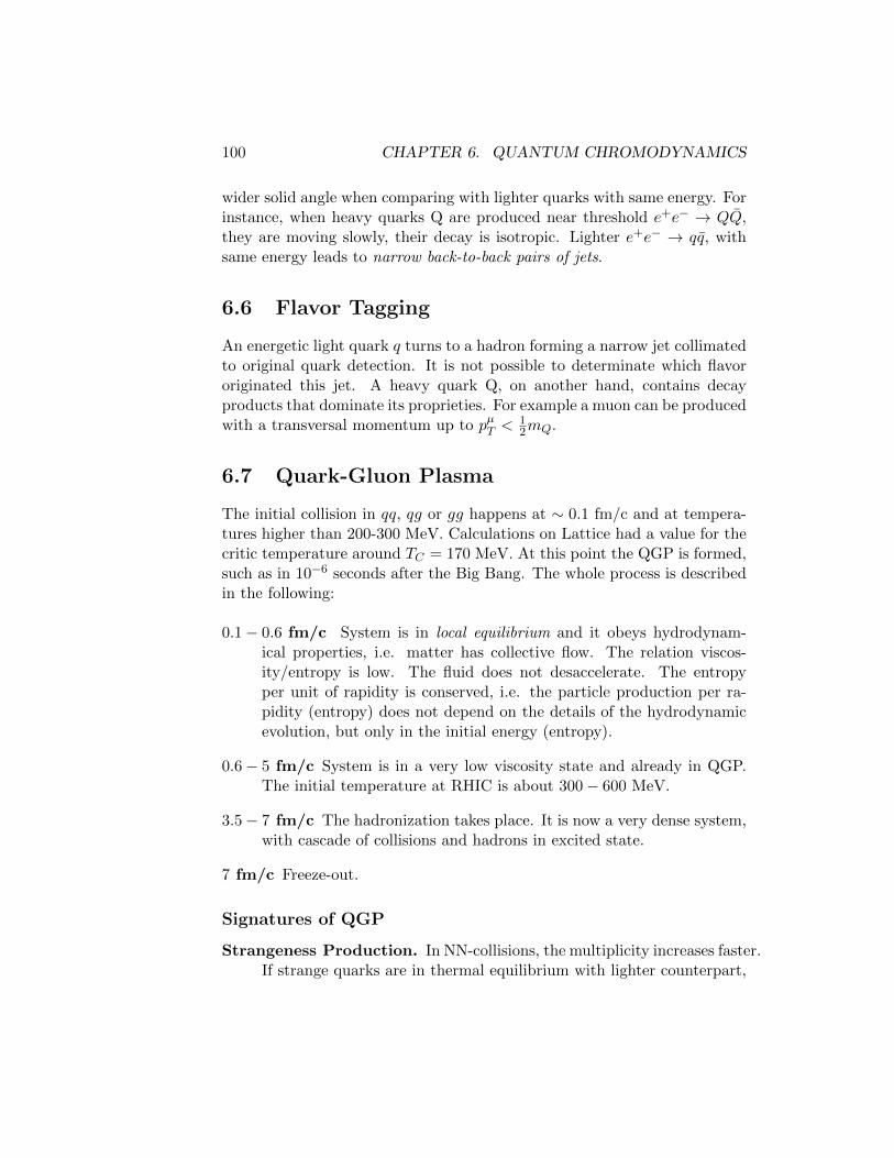
100 CHAPTER 6. QUANTUM CHROMODYNAMICS
wider solid angle when comparing with lighter quarks with same energy. Forinstance, when heavy quarks Q are produced near threshold e+e− → QQ,they are moving slowly, their decay is isotropic. Lighter e+e− → qq, withsame energy leads to narrow back-to-back pairs of jets.
6.6 Flavor Tagging
An energetic light quark q turns to a hadron forming a narrow jet collimatedto original quark detection. It is not possible to determinate which flavororiginated this jet. A heavy quark Q, on another hand, contains decayproducts that dominate its proprieties. For example a muon can be producedwith a transversal momentum up to pµT <
12mQ.
6.7 Quark-Gluon Plasma
The initial collision in qq, qg or gg happens at ∼ 0.1 fm/c and at tempera-tures higher than 200-300 MeV. Calculations on Lattice had a value for thecritic temperature around TC = 170 MeV. At this point the QGP is formed,such as in 10−6 seconds after the Big Bang. The whole process is describedin the following:
0.1− 0.6 fm/c System is in local equilibrium and it obeys hydrodynam-ical properties, i.e. matter has collective flow. The relation viscos-ity/entropy is low. The fluid does not desaccelerate. The entropyper unit of rapidity is conserved, i.e. the particle production per ra-pidity (entropy) does not depend on the details of the hydrodynamicevolution, but only in the initial energy (entropy).
0.6− 5 fm/c System is in a very low viscosity state and already in QGP.The initial temperature at RHIC is about 300− 600 MeV.
3.5− 7 fm/c The hadronization takes place. It is now a very dense system,with cascade of collisions and hadrons in excited state.
7 fm/c Freeze-out.
Signatures of QGP
Strangeness Production. In NN-collisions, the multiplicity increases faster.If strange quarks are in thermal equilibrium with lighter counterpart,

6.7. QUARK-GLUON PLASMA 101
the ratio of the strange to non strange has an enhancement comparedto non-equilibrium situations.
Suppression of J/ψ and ψ production. Because of the color screening,the interaction between c and c is diminished by the presence of otherquarks.
Two particle interferometry.
Thermal Radiation.
Dilepton Production.

102 CHAPTER 6. QUANTUM CHROMODYNAMICS

Chapter 7
Renormalization
7.1 Gamma and Beta Functions
The gamma function is defined as
Γ(z) =
∫ ∞0
dxxz−1,
<z > 0.
This integral does not exist for <z < 0. We have the following propri-eties,
zΓ(z) = Γ(1 + z),
Γ(z − 1) =Γ(z)
z − 1,
where Γ(z) has isolated points at negative integers and z = 0. We can show
the residue of the pole at z = −N is (−1)N
N ! .
The beta function is defined as
B(µ, ν) =Γ(µ)Γ(ν)
Γ(µ+ ν),
B(µ, ν) =
∫ 1
0dxxµ−1(1− x)y−1,
=
∫ ∞0
dyyν−1(1 + y)−µ−ν ,
= 2
∫ π/2
0dθ(sinθ)2µ−1(cosθ)2ν−1.
103
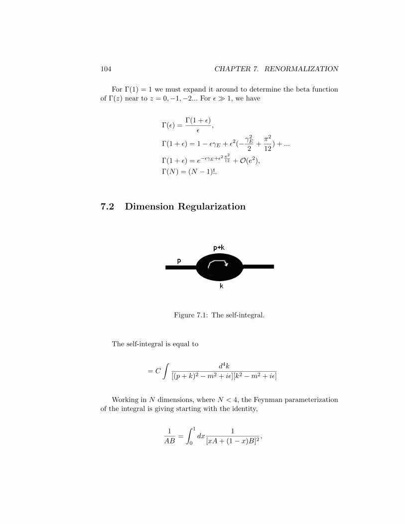
104 CHAPTER 7. RENORMALIZATION
For Γ(1) = 1 we must expand it around to determine the beta functionof Γ(z) near to z = 0,−1,−2... For ε 1, we have
Γ(ε) =Γ(1 + ε)
ε,
Γ(1 + ε) = 1− εγE + ε2(−γ2E
2+π2
12) + ...
Γ(1 + ε) = e−εγE+ε2 π2
12 +O(e2),
Γ(N) = (N − 1)!.
7.2 Dimension Regularization
Figure 7.1: The self-integral.
The self-integral is equal to
= C
∫d4k
[(p+ k)2 −m2 + iε][k2 −m2 + iε]
Working in N dimensions, where N < 4, the Feynman parameterizationof the integral is giving starting with the identity,
1
AB=
∫ 1
0dx
1
[xA+ (1− x)B]2,

7.2. DIMENSION REGULARIZATION 105
where
In(p2) =
∫d4k
[(p+ k)2 −m2 + iε]
1
[k2 −m2 + iε],
=
∫dnk
∫ 1
0
dk
[x(p+ k)2 − xm2 + (1− x)k2 − (i− x)m2 + iε[x+ (1− x)]]2,
=
∫ 1
0
∫dnk
1
[k2 + 2pxk + xp2 −m2 + iε]2,
=
∫ 1
0dx
∫dn−1~l
∫dl0
[l20 − l2 + x(1− x)p2 −m2 + iε]2,
in the last, the square was completed.Poles are at l0 = ±
√l2 − x(1− x)p2 +m2 − iε, as long as p2 < 4m2.
We then choose to perform the integral by Wick rotation and the originalcontour turns to a closed contour with no poles (-i∞ to i∞). From Cauchy,∫ ∞
−∞C1
dl0 =
∫ ∞−∞C2
dl0,
lη = il0,∫ ∞−∞
dl0 = i
∫ ∞−∞
dlη.
Along C2 we get
Iη(p2) = i
∫ 1
0dx
∫ ∞−∞
dn−1ldln[−l2n − l2 −m2 + x(1− x)p2]−2,
Now, in polar coordinates in N (now Euclidean) dimensions, choosingN = 2, ∫
dl2dl1 =
∫ ∞0
dll
∮ 2π
0dφ,
(l2 = l22 + l21),
I2(p2) = 2πi
∫ 1
0dx
∫ ∞0
dll
[l2 +m2 − x(1− x)p2]2,
= πi
∫ 1
0dx
1
[m2 − x(1− x)p2]2,
=−iπp2
1√1− 2m2
p2
ln
(√1− 4m2
p2− 1√
1− 4m2
p2+ 1
).

106 CHAPTER 7. RENORMALIZATION
The Wick rotation defines the integral where it is analytical, findingbranch cuts by continuation. A branch cut at two-particle threshold isp2 ≥ 4m2. This method is completely general, for any Green’s functionGl(p1...pl), if one starts with p2
i < 0 and also∑p2i < 0 (no exceptional
momenta). Then, for this case, diagrams can be Wick-rotated diagram bydiagram doing all loop diagrams to get all the analytical diagrams.
The generalization of Feynman parameters is (the integral in D dimen-sions) is
1∏Ai=1(Di + iε)si
=Γ(∑A
i=1 si)∏Ai=1 Γ(si)
∫ 1
0
sx1dx2..dxA
[∑A
i=1 xiDi + iε]∑siδ(1−
A∑i=1
xi)A∏i=1
xs−1i .
It reduces to the previous case and makes it possible to organize thedenominator in the loop momenta. Formally, the steps are
• Exchanging k, exchanges xi (the integral must be convergent for thischange, and this is the importance of the dimension regularization).
• Complete the squares.
• Wick rotation (ld = il0).
• Put in polar coordinates.
• This gives ID(pi, σi) = i(−1 + iε)−s, assuming the remaining integralis real.
ID(pi, σi, xi) =
∫dΩD−1
∫ ∞0
dllD−1
[l2 +M2]∑σi,
m2 =
s∑i=1
xi(
i∑σ=1
pi)2 − (
i∑i=1
xi
i∑l=1
pl)2
The radial integral is ∫ ∞0
dllD−1
[l2 +M2]∑σi,
with a change of variable y = l0/√M2 and then y2 = η, we have finally∫ ∞
0
dllD−1
[l2 +M2]∑σi
= (M2)D2−∑σi
1
2B(
D
2,∑i
σi −D
2).
From diagrams with self-energy, σ1 6= 1. The poles are

7.2. DIMENSION REGULARIZATION 107
• For D ≤ 2∑
∆i, D ≤ 0.
• The radial integral applies any D ∈ C.
The angular integral is evaluated by changing to the cylindrical coordi-nates in k 6= 1 dimensions∫
dk+1q =
∫ ∞−∞
dzk+1
∫dkq,
=
∫ ∞−∞
dzk+1
∫dqqk−1
∫dΩk−1,
defining qk+1 =√z2k+1 + q2
k, cosθw = zz+1
qk+1, we get
∫dk+1q =
∫dqk+1q
kk+1
∫ π
0dθk sink−1θk
∫dΩk−1,
=
∫dqk+1q
kk+1
∫dΩk,
ΩD−1 =2πD/2
Γ(D2,
where πD2 = (Γ(1
2))D.
Gathering everything together,
ID(pi, σi) =
i(−i+ iε)−∑σi
1
πγ(σi)
∫ 10
∏i dxi δ(1−
∑xi)x
σi−1i Γ(
∑σi −
D
2)π
D2 [M2(pi, xi,mi)]
D2−∑i σi .
The basic integral is obtained doing si = 1 and defining∑
i si = s
JD,s(q2,M2) = Γ(s)
∫dDk
(2π)D1
[k2 + 2kq −M2 − iε]s
=i(−1)s
(4π)D2
Γ(s− D
2)(q2 +M2 − iε)
D2−s.
Inside the Feynman parameters integral, one starts with D < 25 andtaking D → 4 finds isolated poles which will be treat by renormalization.

108 CHAPTER 7. RENORMALIZATION
Example: The φ34-Theory
The loop integral is equal to
Σ0(p2,m2) = (+i)(−ig0)2i21
2,
=
∫dDk
(2π)D1
k2 −m2 − iε1
(p− k)2 −m2 + iε,
=ig2
0
∈
1
0dxJD/2((xp)2,m2 − xp2),
=(i)2g2
0
2(4π)D2
Γ(2− D
2)
∫ 1
0
[m2 − x(1− x)p2 − iε
].
Separating the poles, which are the ultraviolet correction, one definesε = 2− D
2 and Γ(ε)→ pole as ε = 0. The expansion of (7.2.1) and isolatingthe pole and the infinite yields
Σ0(p2,m2) = − g20
2(4π)2(1− ε ln 4π + ...)(
1
ε− γE ...)(
∫ 1
0dx− ε
∫ 1
0dx ln ...),
where we neglect terms that vanish when ε→ 0 and almost everything can-cels. Problems with this equation is that this pole, however, is divergent forD = 4 and there is no scale for logarithm, necessitating the renormalization.
7.3 Terminology for Renormalization
• 1PI diagrams: either vertices or loop diagrams, all ultraviolet diver-gences are 1PI divergences.
• Notation: ΓN = −iγN , where for N > 2 it is just the sum of 1PIdiagram.
• For the special case N=2, one has Γ = p2 − m2 − iγ2 = p2 − m2 −iΣ(p2,m2).
• The Green’s function is G2 = iΓ2
= ip2−m2−Σ(p2,m2)
. The pole in
this function is the physical mass but not necessary the same of theFeynman propagators.

7.4. CLASSIFICATION OF DIAGRAMS FOR SCALAR THEORIES 109
7.4 Classification of Diagrams for Scalar Theories
For a D-Dimensional φP theory, one has
• L - loop.
• E - external lines
• N - lines
• DL - number of integrals
Looking for superficial overall degree of divergence, all loop momentagoes to infinity at once, one has:
γE =∑1PI
∈L∏
2−1 loops
dDkl
N∏k=1
1
[q2]
The superficial degree of divergence is
ω(ΓE) = DL− 2N.
• ω(ΓE) < 0, superficially convergent,
• ω(ΓE) > 0, superficially power divergent, ω(ΓE) = 0, superficially logdivergent.
One fixes D, chooses p (power of the theory and then ω does not dependon the powers of the diagram), and then finds them in function of E and V ,
L = N − V − 1,
pV = 2N + E.
Together with (7.4.1), one has for each diagram the algebraic function,
ω(ΓE) = D − E(D − 2
2) + V (
p
2(D − 2)−D),
where only the last term depends on the order. There are then three cases,
1. p(D−22 )−D < 0, better convergence as order increase (super-renormalizable),
for example for p = 3 and d = 4.
2. p(D−22 )−D > 0, convergence gets worse as V increases (non-renormalizable).

110 CHAPTER 7. RENORMALIZATION
3. p(D−22 ) −D = 0, ω(ΓE) ≥ 0 only for finite number of E (renormaliz-
able).
The dimensionality of the Lagrangian is then calculated as
L =1
2LKG −
g
p!φp,
in D dimensions (natural units) one has
[L] = 1,
[∂x] = [m] = 1,
[φ] =D − 2
2,
[g] = D − p(D − 2
2) = D − p[φ].
In terms of ω:
ω(ΓE) = D − E[φ]− V [g],
where
1. [g] > 0 superrernomalizable (φ34).
2. [g] = 0 superrernomalizable (φ36, φ
44).
3. [g] > 0 superrernomalizable (φ46).
Now one makes the D-dependence of g explicitly introducing a new massscale M ,
L =1
2LKG −
gM ε
p!φp,
where for D = 4 one has [g] = [M ε] = massε, ε = 2− D2 .
Other example, for a 6-theory, results in −gMε
3! φ36, where ε = 3− D
2 . Fora gauge theory, ε = 2− D
2 .
7.5. RENORMALIZATION FOR φ34 111
7.5 Renormalization for φ34
From (7.2.1), defining gεµ = g0,
Σ0(p2,m2) =g2
0
2(4π)2[1
ε− γE + ln 4π −
∫ 1
0dx ln (m2 − x(1− x)φ2 − iε)...],
=g2
0
2(4π)2[1
ε− γE + ln 4π −
∫ 1
0dx ln (
m2
M2− x(1− x)
p2
M2− iε) + ...]
where M is the renormalization mass (and an arbitrary constant) and therest of the equation vanish for ε→ 0. The logarithm function is dimension-less but the ultraviolet divergence is
• Additive to finite terms.
• Independent of p (it is local, correspond to a well-defined point).
• Simplly g2
s(4π)21ε .
These proprieties allow us to remove the divergence by renormaliza-tion which is the modification of the Lagrangian with the new local terms.The counterterms are designed to cancel poles in ε. The polynomials inp corresponds to derivatives of the field (which will appear in the generalcases). One then defines Lren → Lclass + Lctr, where Lctr = −1
2δm2φ2 and
δm2 = − g2
2(4π)2(−1
ε + cm), and this last part is the sum of poles plus an
arbitrary part.The new terminology is given by
• δm2 os the mass shift.
• cm is the constant that defines the renormalization scheme.
The new lagrangian, Lctr, is treated as a new vertex in perturbationtheory, presented as the figure 7.2, and it can be work out in the momentaspace.
= −i(2π)4δ4(p− p′)δm2.
Computing Γ2 in the order g2 one has
Γ2 =g
2(2π)4[cm − γE + ln 4π −
∫ 1
0dx ln (
m2
M2− x(1− x)
p2
M2− iε)],
resulting that ε→ 0 when D → 4.The classification of the theory, depending on cm, is given by
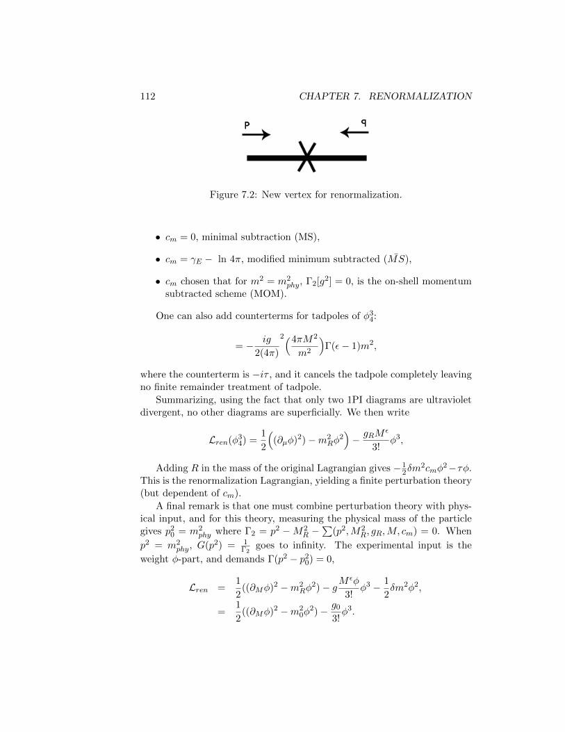
112 CHAPTER 7. RENORMALIZATION
Figure 7.2: New vertex for renormalization.
• cm = 0, minimal subtraction (MS),
• cm = γE − ln 4π, modified minimum subtracted (MS),
• cm chosen that for m2 = m2phy, Γ2[g2] = 0, is the on-shell momentum
subtracted scheme (MOM).
One can also add counterterms for tadpoles of φ34:
= − ig
2(4π)
2(4πM2
m2
)Γ(ε− 1)m2,
where the counterterm is −iτ , and it cancels the tadpole completely leavingno finite remainder treatment of tadpole.
Summarizing, using the fact that only two 1PI diagrams are ultravioletdivergent, no other diagrams are superficially. We then write
Lren(φ34) =
1
2
((∂µφ)2)−m2
Rφ2)− gRM
ε
3!φ3,
Adding R in the mass of the original Lagrangian gives −12δm
2cmφ2−τφ.
This is the renormalization Lagrangian, yielding a finite perturbation theory(but dependent of cm).
A final remark is that one must combine perturbation theory with phys-ical input, and for this theory, measuring the physical mass of the particlegives p2
0 = m2phy where Γ2 = p2 −M2
R −∑
(p2,M2R, gR,M, cm) = 0. When
p2 = m2phy, G(p2) = 1
Γ2goes to infinity. The experimental input is the
weight φ-part, and demands Γ(p2 − p20) = 0,
Lren =1
2((∂Mφ)2 −m2
Rφ2)− gM
εφ
3!φ3 − 1
2δm2φ2,
=1
2((∂Mφ)2 −m2
0φ2)− g0
3!φ3.

7.6. GUIDELINE FOR RENORMALIZATION 113
The final important result is
Lren = Lbarl(m0, g0),
where from
1. LHS, the perturbation theory is in term ofm2R, g
2R = g0M
ε = m20+δm2,
and it is finite order by order in perturbation theory (every divergentdiagram is canceled).
2. RHS, the perturbation theory only depends on two parameters.
From item 1, one picks cm and a value for M , then the Green’s functionare ultraviolet finite but depend on cm and M .
From item 2, choices on cm and M only affects the relation between mp
and mphy. Once one knows mR for some M , it is possible to calculate allremaining Green’s function for the S-matrix.
7.6 Guideline for Renormalization
This steps are for λψ3, d = 6, ω(Γ) = 6− 2N , however they give the routefor farther process of renormalization,
1. The Lagrangian is L = 12∂µψ∂µψ−
12m
2ψ2+ λ3!ψ
3. One has two graphicsand since ω(Γ) > 0, they might be divergent.
2. Introduce a new coupling λ→ λδ(N,d)µ , in the new dimension N ∼ d+ε.
In this case δ = −12(N − d) = 1
2N + 3 = ε, thus ε = 3 − n2 and one
rewrites λ→ λεµ.
3. From drawing the diagram one has
=λ2µ2ε
(2π)N
∫dnl
(l −m2)((p− l)2 −m2).
4. Wick rotating (the momentum becomes imaginary):
=λ2µ2ε
(2π)N
∫dN l
(−l2 −m2)(−(p− l)2 +m2).
5. Using the Feynman relation 1AB =
∫ 1o dx
1(xA+(1−x)B)2
, gives
=(λµε)
(2π)N
∫ 1
0dx
∫dN l
(2π)N1
x(l2 +m2 + (1− x))((l − p) +m2)2.

114 CHAPTER 7. RENORMALIZATION
6. With the variable change l′ = l − lp(1− x) to get read of the l termswhen squaring l′, yields
=λ2µ2ε
(2π)N
∫ 2
odx
∫dN l
(l′2 +m2 + p2(1− x)x)2.
7. The solution of this integral is given by∫dN l
(2π)N
( 1
(l2 −M2)A
)=
Γ(A− n2 )
(2π)N2 Γ(A)
1
(M2)A−12
.
Resulting in
=λ2µ2ε
(2π)12
Γ(2− n2 )
2
∫ 1
odx
1
(m2 + p2x(1− x(1− x))2−n/2 .
8. Performing n2 = 3− ε, results on Γ(2− N
2 ) = Γ(−1 + ε). The integralis then
=λ2µ2ε
(2π)12
Γ(ε− 1)
2
∫ 1
0dx
1
(m2 + p2x(1− x))ε−1.
9. The next step is to subtract the divergences using Γ(ε−N) = 1ε − γE ,
resulting on
=λ2µ2ε
(2π)N2
Γ(ε− 1)
2
∫ 1
0dx
m2 + p2x(1− x)
(m2 + p2x(1− x))ε.
10. From the expansion aε = 1 + ε ln a and some algebra finally gives thedivergent term in first order,
=λ2
(2π)3
1
2(m2 +
4
3p2)
1
ε+O(ε).
The counter-terms are always proportional to m2, p2 and λ.
Chapter 8
Sigma Model
115

116 CHAPTER 8. SIGMA MODEL

Part II
Topological Field Theories
117


Bibliography
[WITTEN1982] Witten, E., Supersymmetry and Morse Theory,J.Diff.Geom. 17 (1982) 661.
[WITTEN1988] Witten, E.Topological Sigma Models, Commun. Math.Phys. 118 (1988) 411.
[WITTEN1998-2] Witten, E., Topological Quantum Field Theory, Com-mun. Math. Phys. 117 (1988) 353.
[WITTEN1989] Witten, E., Quantum Field Theory and The Jones Polyno-mial, Commun. Math. Phys. 121 (1989) 351.
[ATIYAH1990] Atiah, The Geometry and Physics of Knots,1990.
[STERMAN1993] Sterman, Quantum Field Theory, 1993.
[PS1995] Peskin and Schroeder; Introduction to Quantum Field Theory,1995.
[ZEE2003] Zee, A.; Quantum Field Theory, 2003.
[LM2005] Labastida and Marino.; Topological Quantum Field Theory, 2005.
[WEINBERG2005] Weinberg, S; Quantum Field Theory I and II, 2005.
[DK2007] Donaldson, S. and Krohnheimer, P.; The Geometry of Four-Manifolds, 2007.
[SREDNICKI2007] Srednicki; Quantum Field Theory, 2007.
[IVANCEVIC2008] Ivancevic; Undergraduate Lecture Notes in TopologicalQuantum Field Theory, http://arxiv.org/abs/0810.0344, 2008.
[KHARZEEV2010] Kharzeev, D.; Graduate Course on Elementary Parti-cles, taught by; Stony Brook University, 2010.
119

Index
Angular Momentum Tensor, 36
Beta Function, 105
Causality, 60Chirality, 53Clifford algebra, 25, 27, 34Completeness Relation, 20Coupling of Fields, 39
QED, 39
Delta Function, 20DGLAP, 95Dirac Equation, 26, 32, 33Dirac Lagrangian, 33
Energy-Moment Tensor, 14Equal-Time Commutators, 16
Anti-commutation, 45
Feynman Identity, 77Feynman Rules
QED, 74Scalar Fields, 23
Fock Space, 19Fourier transformations, 18Free Particle, 12
Gamma Function, 105Gauge Fixing
Lorentz Gauge, 38Gauge Groups
Sl(2,C), 29Sl(N), 64
SO(N), 64SU(N), 35, 64U(1), 15, 32, 35, 46, 64U(N), 37, 61SU(2), 29
Generating Function, 22Global Symmetry, 37Grassmanian Variables, 49Green’s Function, 21, 71Gross-Neveu Model, 89
Higgs Boson, 85Higgs Mechanism
SU(2)× U(1), 66
Jet, 90, 100
Klein-Gordon Equation, 12, 26, 32,46, 57
Lagrange’s Equations of Motion, 12Lie Algebra
Compact, 63Light-Cone Coordinates, 47
Mandelstam Variables, 82Minimal Coupling, 39Momentum-Energy Tensor, 36
Noether’s Theorem, 13Dirac Lagrangian, 35
OperatorAngular Momentum, 46
120

INDEX 121
Casimir, 29, 37, 66Creating and Annihilation, 45Creation and Annihilation, 18, 50Number, 19Projective, 38
Optical Theorem, 78
Parity, 37, 55Weyl Lagrangian, 37
Parton, 89Path Integral, 22
QED, 73Pauli Matrices, 25, 29Pauli-Lobanski vector, 36Poincare Group, 15Principle of Minimum Action, 12Proca Field, 38, 46, 68
QCD, 87QED, 39, 88Quantization, 11, 16, 44Quark-Gluon-Plasma, 102
Reduction Theorem, 22
S-Matrix, 20, 71, 75Bhabha Scattering, 75Compton Scattering, 75
Spin-Statistic Theorem, 25, 46, 60Spinors, 29
Majorana, 32Weyl, 30
Spontaneous Symmetry Breaking, 66
T-Matrix, 21, 75Tachyons, 42Transition Amplitude, 21
UnitaryTransformations, 17
Vector Fields, 31
Weyl Equation, 32Wick Rotation, 23, 107Wigner
Boost, 40Little Group, 40, 47Method, 40, 46
Yang-MillsFields, 61