Embed Size (px)
Citation preview

default
Introduction to PyLith v3.0
Brad Aagaard
June 10, 2019

default
PyLithA modern, community-driven code for crustal deformation modeling
DevelopersBrad Aagaard (USGS)Matthew Knepley (Univ. of Buffalo)Charles Williams (GNS Science)
Combined dynamic modeling capabilities of EqSim (Aagaard) with thequasi-static modeling capabilities of Tecton (Williams)Use modern software engineering to develop an open-source, community code
Modular designTestingDocumentationDistribution
PyLith v1.0 was released in 2007
Introduction

default
Crustal Deformation ModelingElasticity problems where geometry does not change significantly
Quasi-static modeling associated with earthquakes
Strain accumulation associated with interseismic deformationWhat is the stressing rate on faults X and Y?Where is strain accumulating in the crust?
Coseismic stress changes and fault slipWhat was the slip distribution in earthquake A?How did earthquake A change the stresses on faults X and Y?
Postseismic relaxation of the crustWhat rheology is consistent with observed postseismic deformation?Can aseismic creep or afterslip explain the deformation?
Introduction

default
Crustal Deformation ModelingElasticity problems where geometry does not change significantly
Dynamic modeling associated with earthquakes
Modeling of strong ground motionsForecasting the amplitude and spatial variation in ground motion for scenarioearthquakes
Coseismic stress changes and fault slipHow did earthquake A change the stresses on faults X and Y?
Earthquake rupture behaviorWhat fault constitutive models/parameters are consistent with the observed rupturepropagation in earthquake A?
Introduction

default
Crustal Deformation ModelingElasticity problems where geometry does not change significantly
Volcanic deformation associated with magma chambers and/or dikesInflation
What is the geometry of the magma chamber?What is the potential for an eruption?
EruptionWhere is the deformation occurring?What is the ongoing potential for an eruption?
Dike intrusionsWhat is the geometry of the intrusion?What is the pressure change and/or amount of opening/dilatation?
Introduction

default
Crustal Deformation ModelingOverview of workflow for typical research problem
GeologicStructure
MeshGeneration
PhysicsCode Visualization
Gocad
Earth Vision
CUBIT/Trelis
LaGriT
TetGen
Gmsh
PyLith
Relax
GeoFEST
Abaqus
ParaView
Visit
Matlab
Matplotlib
GMT
CIG
Open Source
Free
Commercial
Available
Planned
Introduction

default
PyLith v3.0
Multiphysics formulation through point-wise integration kernelsHigher order spatial and temporal discretizationsAdaptive time stepping via PETSc TSImproved fault formulation for spontaneous rupture (coming in v3.1)Many other small changes
PyLith v3.0

default
Aside: Finite-Element MethodStrong form to weak form
Solve governing equation in integrated sense:∫Ωψtrial · PDE dΩ = 0, (1)
by minimizing the error with respect to the unknown coefficients.
This leads to equations of the form:∫Ωψtrial · f0(x, t) +∇ψtrial · f1(x, t) dΩ = 0. (2)
PyLith v3.0

default
Governing Equations
We want to solve equations in which the weak form can be expressed asF (t, s, s) = G(t, s) (3)
s(t0) = s0 (4)where F and G are vector functions, t is time, and s is the solution vector.
Using the finite-element method and divergence theorem, we cast the weak form into∫Ω
~ψtrial · ~f0(t, s, s) +∇~ψtrial : f1(t, s, s) dΩ =∫Ω
~ψtrial · ~g0(t, s) +∇~ψtrial : g1(t, s) dΩ, (5)
where ~f0 and ~g0 are vectors, and f1 and g1 are tensors.
PyLith v3.0

default
Explicit Time Stepping
Explicit time stepping with the PETSc TS requires F (t, s, s) = s.
Normally F (t, s, s) contains the inertial term (ρu).
Therefore, we transform our equation into the form:F ∗(t, s, s) = s = G∗(t, s) (6)
s = M−1G(t, s). (7)
PyLith v3.0

default
Solving the EquationsExplicit time stepping requires a subset of the terms used in implicit time stepping.
PETSc TS object provides time-stepping and solver implementationsApplication code provides functions for computing RHS and LHS residuals andJacobians
Explicit time steppingCompute RHS residual, G(t, s)Compute lumped inverse of LHS, M−1
No need to compute LHS residual, because F (t, s, s) = s
Implicit time stepping (Krylov solvers)Compute RHS residual, G(t, s)Compute LHS residual, F (t, s, s)Compute RHS Jacobian, JG = ∂G
∂s
Compute LHS Jacobian, JF = ∂F∂s + stshift
∂F∂s
PyLith v3.0

default
Example: Elasticity with Prescribed SlipUse domain decomposition and Lagrange multipliers to prescribe slip
Implicit time stepping without inertia
~sT = (~u ~λ)T , (8)~0 = ~f(~x, t) + ∇ · σ(~u) in Ω, (9)
σ · ~n = ~τ(~x, t) on Γτ , (10)~u = ~u0(~x, t) on Γu, (11)~0 = ~d(~x, t)− ~u+(~x, t) + ~u−(~x, t) on Γf , (12)
σ · ~n = −~λ(~x, t) on Γf+ , (13)
σ · ~n = +~λ(~x, t) on Γf− . (14)
Governing Equations Elasticity

default
Example: Elasticity with Prescribed Slip (cont.)
We create the weak form by taking the dot product with the trial function ~ψutrial or~ψλtrial and integrating over the domain:
0 =
∫Ω
~ψutrial ·(~f(t) + ∇ · σ(~u)
)dΩ, (15)
0 =
∫Γf
~ψλtrial ·(~d(~x, t)− ~u+(~x, t) + ~u−(~x, t)
)dΓ. (16)
Using the divergence theorem and incorporating the Neumann boundary and faultinterface conditions, we can rewrite the first equation as
0 =
∫Ω
~ψutrial · ~f(t) +∇~ψutrial : −σ(~u) dΩ +
∫Γτ
~ψutrial · ~τ(~x, t) dΓ
+
∫Γf
~ψu+
trial · −~λ(~x, t) + ~ψu−
trial ·+~λ(~x, t) dΓ.(17)
Governing Equations Elasticity

default
Example: Elasticity with Prescribed Slip (cont.)
Identifying F (t, s, s) and G(t, s), we haveF u(t, s, s) = 0, (18)
F λ(t, s, s) = 0, (19)
Gu(t, s) =
∫Ω
~ψutrial · ~f(~x, t)︸ ︷︷ ︸gu0
+∇~ψutrial : −σ(~u)︸ ︷︷ ︸gu1
dΩ (20)
+
∫Γτ
~ψutrial · ~τ(~x, t)︸ ︷︷ ︸gu0
dΓ +
∫Γf
~ψu+
trial · −~λ(~x, t)︸ ︷︷ ︸gu
+
0
+ ~ψu−
trial ·+~λ(~x, t)︸ ︷︷ ︸gu
−0
dΓ, (21)
Gλ(t, s) =
∫Γf
~ψλtrial ·(~d(~x, t)− ~u+(~x, t) + ~u−(~x, t)
)︸ ︷︷ ︸
gλ0
dΓ. (22)
Governing Equations Elasticity

default
Example: Elasticity with Prescribed Slip (cont.)
JuuG =∂Gu
∂u=
∫Ω∇~ψutrial :
∂
∂u(−σ) dΩ =
∫Ω∇~ψutrial : −C :
1
2(∇+∇T )~ψubasis dΩ
=
∫Ωψvtrial i,k (−Cikjl)︸ ︷︷ ︸
Juug3
ψubasis j,l dΩ(23)
JuλG =∂Gu
∂λ=
∫Γf+
~ψutrial ·∂
∂λ(−~λ) dΓ +
∫Γf−
~ψutrial ·∂
∂λ(+~λ) dΓ
=
∫Γf
ψu+
trial i −1︸︷︷︸Ju
+λg0
ψλbasis j + ψu−
trial i +1︸︷︷︸Ju
−λg0
ψλbasis j dΓ(24)
JλuG =∂Gλ
∂u=
∫Γf
~ψλtrial ·∂
∂u
(~d(~x, t)− ~u+(~x, t) + ~u−(~x, t)
)dΓ
=
∫Γf
ψλtrial i( −1︸︷︷︸Jλu
+
g0
)ψu+
basis j + ψλtrial i( +1︸︷︷︸Jλu
−g0
)ψu−
basis j dΓ(25)
JλλG = 0 (26)Governing Equations Elasticity

default
Example: Incompressible Elasticity
Implicit time stepping without inertia~sT = (~u p)T , (27)
~0 = ~f(t) + ∇ ·(σdev (~u)− pI
)in Ω, (28)
0 = ~∇ · ~u+p
K, (29)
σ · ~n = ~τ on Γτ , (30)~u = ~u0 on Γu, (31)p = p0 on Γp. (32)
Governing Equations Incompressible Elasticity

default
Example: Incompressible Elasticity (cont.)
Using trial functions ~ψutrial and ψptrial and incorporating the Neumann boundaryconditions:
0 =
∫Ω
~ψutrial · ~f(t) +∇~ψutrial :(−σdev (~u) + pI
)dΩ +
∫Γτ
~ψutrial · ~τ(t) dΓ, (33)
0 =
∫Ωψptrial ·
(~∇ · ~u+
p
K
)dΩ. (34)
Identifying G(t, s), we have
0 =
∫Ω
~ψutrial · ~f(t)︸︷︷︸gu0
+∇~ψutrial :(−σdev (~u) + pI
)︸ ︷︷ ︸
gu1
dΩ +
∫Γτ
~ψutrial · ~τ(t)︸︷︷︸gu0
dΓ, (35)
0 =
∫Ωψptrial ·
(~∇ · ~u+
p
K
)︸ ︷︷ ︸
gp0
dΩ. (36)
Governing Equations Incompressible Elasticity

default
Example: Incompressible Elasticity (cont.)
With two fields we have four Jacobians for the RHS associated with the coupling ofthe two fields.
JuuG =∂Gu
∂u=
∫Ω∇~ψutrial :
∂
∂u(−σdev ) dΩ =
∫Ωψutrial i,k
(−Cdev
ikjl
)︸ ︷︷ ︸
Juug3
ψubasis j,l dΩ (37)
JupG =∂Gu
∂p=
∫Ω∇~ψutrial : Iψpbasis dΩ =
∫Ωψutrial i,k δik︸︷︷︸
Jupg2
ψpbasis dΩ (38)
JpuG =∂Gp
∂u=
∫Ωψptrial
(~∇ · ~ψubasis
)dΩ =
∫Ωψptrial δjl︸︷︷︸
Jpug1
ψubasis j,l dΩ (39)
JppG =∂Gp
∂p=
∫Ωψptrial
1
K︸︷︷︸Jppg0
ψpbasis dΩ (40)
Governing Equations Incompressible Elasticity

default
Summary of Multiphysics Implementation
We decouple the element definition from the fully-coupled equation, using pointwisekernels that look like the PDE.
Flexibility The cell traversal, handled by the library, accommodates arbitrary cellshapes. The problem can be posed in any spatial dimension with anarbitrary number of physical fields.
Extensibility The library developer needs to maintain only a single method, easinglanguage transitions (CUDA, OpenCL). A new discretization schemecould be enabled in a single place in the code.
Efficiency Only a single routine needs to be optimized. The application scientist isno longer responsible for proper vectorization, tiling, and other traversaloptimization.
Governing Equations Incompressible Elasticity

default
Overview of PyLith Workflow
PyLith
Mesh Generator Simulation Parameters
Visualization
Post-processing
CUBIT / Trelis
Exodus file [.exo]
LaGriT
GMV File [.gmv]
Pset File [.pset]
Text Editor
ASCII File [.mesh]
Text Editor
Parameter
File(s) [.cfg]
Spatial
Database(s)
[.spatialdb]
VTK File(s) [.vtk]
HDF5 File(s) [.h5]
Xdmf File(s)
[.xmf]
ParaView Visit
Python w/h5py
Matlab
Using PyLith
default
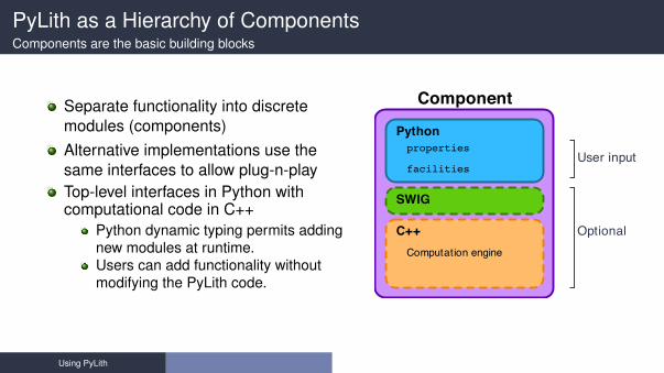
PyLith as a Hierarchy of ComponentsComponents are the basic building blocks
Separate functionality into discretemodules (components)Alternative implementations use thesame interfaces to allow plug-n-playTop-level interfaces in Python withcomputational code in C++
Python dynamic typing permits addingnew modules at runtime.Users can add functionality withoutmodifying the PyLith code.
Using PyLith

default
Parameter FilesSimple syntax for specifying parameters for properties and components
# Syntax
[pylithapp.COMPONENT.SUBCOMPONENT] ; Inline comment
COMPONENT = OBJECT
PARAMETER = VALUE
# Example
[pylithapp.mesh_generator] ; Header indicates path of mesh_generator in hierarchy
reader = pylith.meshio.MeshIOCubit ; Use mesh from CUBIT/Trelis
reader.filename = mesh_quad4.exo ; Set filename of mesh.
reader.coordsys.space_dim = 2 ; Set coordinate system of mesh.
[pylithapp.problem.solution_outputs.output] ; Set output format
writer = pylith.meshio.DataWriterHDF5
writer.filename = axialdisp.h5
[pylithapp.problem]
bc = [x_neg , x_pos , y_neg] ; Create array of boundary conditions
bc.x_neg = pylith.bc.DirichletTimeDependent ; Set type of boundary condition
bc.x_pos = pylith.bc.DirichletTimeDependent
bc.y_neg = pylith.bc.DirichletTimeDependent
[pylithapp.problem.bc.x_pos] ; Boundary condition for +x
constrained_dof = [0] ; Constrain x DOF
label = edge_xpos ; Name of nodeset from CUBIT/Trelis
db_auxiliary_fields = spatialdata.spatialdb.SimpleDB ; Set type of spatial database
db_auxiliary_fields.label = Dirichlet BC +x edge
db_auxiliary_fields.iohandler.filename = axial_disp.spatialdb ; Filename for database
Using PyLith

default
Parameters Graphical User-Interfacecd parametersgui; ./pylith paramviewer
Using PyLith

default
Spatial DatabasesUser-specified field/value in space for properties and BC values.
ExamplesUniform value for Dirichlet BC (0-D)Piecewise linear variation in tractions for Neumann BC (1-D)SCEC CVM-H seismic velocity model (3-D)
Generally independent of discretization for problemAvailable spatial databasesUniformDB Optimized for uniform valueSimpleDB Arbitrarily distributed points for variations in 0-D, 1-D, 2-D, or 3-D
SimpleGridDB Logically gridded points for variations in 0-D, 1-D, 2-D, or 3-DSCECCVMH SCEC CVM-H seismic velocity model v5.3
ZeroDB Special case of UniformDB with zero values
Using PyLith

default
PyLith Design: Focus on GeodynamicsLeverage packages developed by computational scientists
PyLith
spatialdataPETSc
Proj.4HDF5NetCDF Pyre numpy
MPIBLAS/LAPACK
Using PyLith

default
PyLith Development Follows CIG Best Practicesgithub.com/geodynamics/best practices
Version ControlNew features are added in separate branches.Use ’master’ branch as stable development branch.
CodingUser-friendly specification of parameters at runtime.Development plan, updated annually.Users can add features or alternative implementations without modifying code.
PortabilityBuild procedure is independent of compilers and optimization flags.Multiple builds (debug/optimized) from same source.
Documentation and User WorkflowExtensive example suite with varying levels of complexity.Changing simulation parameters does not require rebuilding.Displays version information via --version command line argument.
Using PyLith

default
Development ToolsLeverage open-source tools for efficient code development.
GitHub Code repository supporting simultaneous, independent implementationof new features.
Doxygen Document parameters and purpose of every object and its functions.CppUnit Test nearly every function in code during development.Travis CI Run tests when code is committed to repository.
gcov Records which lines of code tests cover.
Using PyLith
default
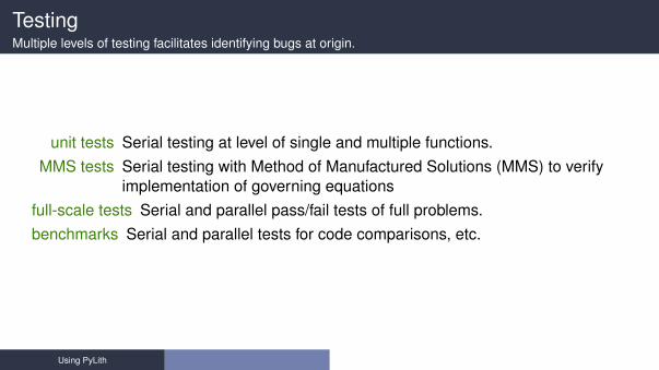
TestingMultiple levels of testing facilitates identifying bugs at origin.
unit tests Serial testing at level of single and multiple functions.MMS tests Serial testing with Method of Manufactured Solutions (MMS) to verify
implementation of governing equationsfull-scale tests Serial and parallel pass/fail tests of full problems.benchmarks Serial and parallel tests for code comparisons, etc.
Using PyLith

default
PyLith v3.0.0beta1 (Jun 10, 2019)Incomplete, contains bugs, but can do interesting physics
Features (mesh importing) not changed remain stable.Some implemented features have been thoroughly tested.Some implemented features have minimal testing.A few implemented features have no testing.Several major features in v2.2 have not yet been implemented.
Using PyLith

default
PyLith v3.0.0beta1: Governing Equations
ElasticityStatic and quasi-static problemsDynamic problems (with inertia)Infinitesimal strainsSmall strainGravitational body forcesBody forcesBulk rheologies (constitutive models)
Isotropic, linear elasticityIsotropic, linear Maxwell viscoelasticityIsotropic, linear generalized Maxwell viscoelasticityIsotropic, power-law viscoelasticityIsotropic, Drucker-Prager elastoplasticity
DoneBuggyIn ProgressComing LaterUsing PyLith

default
PyLith v3.0.0beta1: Governing EquationsIncomplete, contains bugs, but can do interesting physics
Incompressible ElasticityStatic and quasi-static problemsInfinitesimal strainsGravitational body forcesBody forcesBulk rheologies (constitutive models)
Isotropic, linear elasticityIsotropic, linear Maxwell viscoelasticityIsotropic, linear generalized Maxwell viscoelasticityIsotropic, power-law viscoelasticity
Using PyLith

default
PyLith v3.0.0beta1: Boundary and Interface Conditions
Boundary conditionsTime-dependent Dirichlet boundary conditionsTime-dependent Neumann (traction) boundary conditionsAbsorbing boundary conditions
Interface conditionsKinematic (prescribed slip) fault interfaces w/multiple rupturesDynamic (friction) fault interfaces
Static frictionLinear slip-weakeningLinear time-weakeningDieterich-Ruina rate and state friction w/ageing law
Using PyLith

default
PyLith v3.0.0beta1: Other Features
Importing meshesLaGriT: GMV/PsetCUBIT/Trelis: Exodus IIASCII: PyLith mesh ASCII format (intended for toy problems only)
Initial conditionsOutput: HDF5 and VTK files
Solution over domainSolution over domain boundarySolution interpolated to user-specified points w/station namesSolution over materials and boundary conditionsState variables (e.g., stress and strain) for each materialFault information (e.g., slip and tractions)
Using PyLith

default
PyLith v3.0.0beta1: Other Features (cont.)
Automatic conversion of units for all parametersParallel uniform global refinementPETSc linear and nonlinear solversOutput of simulation progress estimates runtime
Using PyLith

default
How do changes from v2.x to v3.x affect users?
No changesMeshesFormats of spatial database files
Substantial changesParameter (cfg) filesNames of values in spatial database files
HDF5 output is now the default
Using PyLith

default
Mesh Generation TipsThere is no silver bullet in finite-element mesh generation
Hex/Quad versus Tet/TriHex/Quad are slightly more accurate and fasterTet/Tri easily handle complex geometryEasy to vary discretization size with Tet, Tri, and Quad cellsThere is no easy answerFor a given accuracy, a finer resolution Tet mesh that varies the discretization sizein a more optimal way might run faster than a Hex mesh
Check and double-check your meshWere there any errors when running the mesher?Are the boundaries, etc marked correctly for your BC?Check mesh quality (aspect ratio should be close to 1)
CUBIT/Trelis General

default
CUBIT/Trelis Workflow
1 Create geometry1 Construct surfaces from points, curves, etc or basic shapes2 Create domain and subdivide to create any interior surfaces
Fault surfaces must be interior surfaces (or a subset) that completely divide domainNeed separate volumes for different constitutive models, not parameters
2 Create finite-element mesh1 Specify meshing scheme2 Specify mesh sizing information3 Generate mesh4 Smooth to fix any poor quality cells
3 Create nodesets and blocks1 Create block for each constitutive model2 Create nodeset for each BC and fault3 Create nodeset for buried fault edges4 Create nodeset for ground surface for output (optional)
4 Export mesh in Exodus II format (.exo files)
CUBIT/Trelis General

default
CUBIT/Trelis IssuesKeep in mind the scales of the observations you are modeling
Topography/bathymetryIgnore topography/bathymetry unless you know it mattersFor rectilinear grid, create UV net surfaceConvert triangular facets to UV net surface via mapped mesh
Fault surfacesBuilding surfaces from contours is usually easiestInclude features at the resolution that matters
PerformanceNumber of points in spline curves/surfaces has huge affect on mesh generationruntimeCUBIT/Trelis do not run in parallelUse uniform global refinement in PyLith for large sims (>10M cells)
CUBIT/Trelis General

default
CUBIT/Trelis Best Practices
Issue: Changes in geometry cause changes in object idsSoln: Name objects and use APREPRO or Python to eliminate hardwired ids
wherever possible
Issue: Splines with many points slows down operationsSoln: Reduce the number of points per spline
Issue: Surfaces meet in small angles creating distorted cellsSoln: Trim geometry to eliminate features smaller than cell size
Issue: Difficulty meshing complex geometry with Hex cellsSoln: Use Tet cells even if it requires a finer mesh
Issue: Hex mesh over-samples parts of the domainSoln: Use Tet mesh and vary discretization within domain
Issue: Extended surfaces create very complex geometrySoln: Subdivide geometry before webcutting to eliminate overly complex
geometryCUBIT/Trelis General

default
PyLith Tips
Read the PyLith User ManualDo not ignore error messages and warnings!Use an example/benchmark as a starting pointQuasi-static simulations
Start with a static simulation and then add time dependenceCheck that the solution converges at every time step
Dynamic simulationsStart with a static simulationShortest wavelength seismic waves control cell size
CIG community forumshttps://community.geodynamics.org/c/pylithPyLith User Resourceshttps://wiki.geodynamics.org/software:pylith:start
CUBIT/Trelis PyLith

default
Getting Started
1 Create a play area for working with examplescd PATH TO PYLITH DIR
mkdir playpen
cp -r src/pylith-3.0.0beta1/examples playpen/
2 Work through relevant examples3 Try to complete relevant exercises listed in the manual4 Modify an example to look like your problem of interest
CUBIT/Trelis PyLith

default
Overview of ExamplesExamples progress from simple to more complex
1 2d/boxAxial compress/extension w/Dirichlet BCShearing with Dirichlet and Neumann BC
2 3d/boxSame as 2d/box in 3D
3 2d/strikeslipVariable mesh size in CUBIT/TrelisPrescribed fault slipDirichlet boundary conditions
4 2d/reverseGravitational body forces with linear elasticityGravitational body forces with incompressible elasticityPrescribed slip on multiple faults
CUBIT/Trelis PyLith

default
Overview of Examples (cont.)Examples progress from simple to more complex
6 2d/subductionMeshing a 2-D cross-section of a subduction zonePrescribed fault slipAfterslip driven by traction changes from coseismic slip
7 3d/strikeslip (wish list)Meshing intersecting strike-slip faults with complex geometryPrescribed fault slip
8 3d/subductionMeshing a 3-D subduction zone with complex geometryPrescribed fault slip
CUBIT/Trelis PyLith