Introduction to programming with Matlab/Python Lecture 2 2/compintro-lecture2.pdf · observing nearby stars one could say something about the rotation curve of ... Performing the

Introduction to programmingwith Matlab/Python

— Lecture 2

Brian Thorsbro

Department of Astronomyand Theoretical Physics,Lund University, Sweden.

Monday, November 6, 2017

Courses

These lectures are a mini-series companion to:

ASTM13 Dynamical Astronomy

ASTM21 Statistical tools in Astrophysics

Matlab installed in the lab (Lyra). Personal laptops are OK!Install Matlab from: http://program.ddg.lth.se/Install Python3 from: https://www.anaconda.com/download/

Brian Thorsbro 1/26

Matlab

Install from: http://program.ddg.lth.se/

Brian Thorsbro 2/26

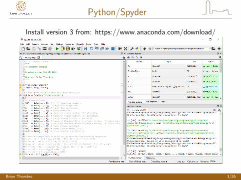
Python/Spyder

Install version 3 from: https://www.anaconda.com/download/

Brian Thorsbro 3/26

Outline

Content in this lecture:

I Finding Oort’s constants(example computational task)

I Least Squares algorithm

I Functions and scope

I Performance

Brian Thorsbro 4/26

The Oort’s constants

In 1927 Jan Oort derived an empirical relation, such that byobserving nearby stars one could say something about the rotationcurve of the Galaxy. The relation is

Acos(2l) + B = Kµl ,

where A says says something about the shearing motion and Bdescribes the rotation of the Galaxy. K is a convenient unittransformation between mas/yr and km/s/kpc which allows us touse the Hipparcos database and compare our results to standardknown values of Oort’s constant (actually using Gaia DR1):

A = 15.3± 0.4 km/s/kpc, B = −11.9± 0.4 km/s/kpc.

(Bovy, 2017)

Brian Thorsbro 5/26

The Hipparcos Database

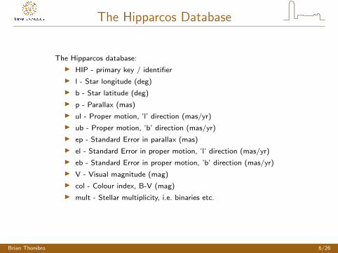
The Hipparcos database:

I HIP - primary key / identifier

I l - Star longitude (deg)

I b - Star latitude (deg)

I p - Parallax (mas)

I ul - Proper motion, ’l’ direction (mas/yr)

I ub - Proper motion, ’b’ direction (mas/yr)

I ep - Standard Error in parallax (mas)

I el - Standard Error in proper motion, ’l’ direction (mas/yr)

I eb - Standard Error in proper motion, ’b’ direction (mas/yr)

I V - Visual magnitude (mag)

I col - Colour index, B-V (mag)

I mult - Stellar multiplicity, i.e. binaries etc.

Brian Thorsbro 6/26

The equation system

With n = 116812 we have a large equation system:

Acos(2l1) + B = Kµl1... =

...

Acos(2ln) + B = Kµln ,

or: cos(2l1) 1...

...

cos(2ln) 1

(A

B

)= K

µl1...

µln

or:

X“design matrix”

(A

B

)= KY

Brian Thorsbro 7/26

Solving the equation system

Naive matrix manipulation suggests:

X

(A

B

)= KY

⇔ XTX

(A

B

)= XTKY

⇔

(A

B

)= (XTX )−1XTKY

Requires that (XTX ) is invertible.

Brian Thorsbro 8/26

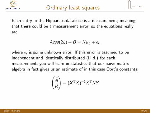
Ordinary least squares

Each entry in the Hipparcos database is a measurement, meaningthat there could be a measurement error, so the equations reallyare

Acos(2li ) + B = Kµli + εi ,

where εi is some unknown error. If this error is assumed to beindependent and identically distributed (i.i.d.) for eachmeasurement, you will learn in statistics that our naive matrixalgebra in fact gives us an estimate of in this case Oort’s constants:(

A

B

)= (XTX )−1XTKY

Brian Thorsbro 9/26

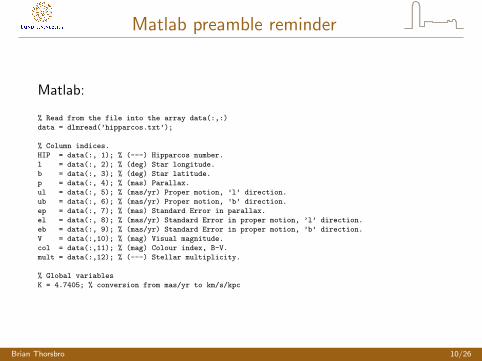
Matlab preamble reminder

Matlab:

% Read from the file into the array data(:,:)

data = dlmread(’hipparcos.txt’);

% Column indices.

HIP = data(:, 1); % (---) Hipparcos number.

l = data(:, 2); % (deg) Star longitude.

b = data(:, 3); % (deg) Star latitude.

p = data(:, 4); % (mas) Parallax.

ul = data(:, 5); % (mas/yr) Proper motion, ’l’ direction.

ub = data(:, 6); % (mas/yr) Proper motion, ’b’ direction.

ep = data(:, 7); % (mas) Standard Error in parallax.

el = data(:, 8); % (mas/yr) Standard Error in proper motion, ’l’ direction.

eb = data(:, 9); % (mas/yr) Standard Error in proper motion, ’b’ direction.

V = data(:,10); % (mag) Visual magnitude.

col = data(:,11); % (mag) Colour index, B-V.

mult = data(:,12); % (---) Stellar multiplicity.

% Global variables

K = 4.7405; % conversion from mas/yr to km/s/kpc

Brian Thorsbro 10/26

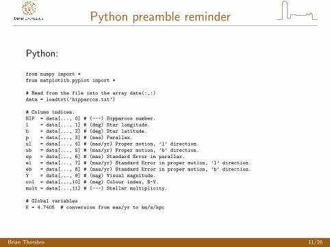
Python preamble reminder

Python:

from numpy import *

from matplotlib.pyplot import *

# Read from the file into the array data(:,:)

data = loadtxt(’hipparcos.txt’)

# Column indices.

HIP = data[..., 0] # (---) Hipparcos number.

l = data[..., 1] # (deg) Star longitude.

b = data[..., 2] # (deg) Star latitude.

p = data[..., 3] # (mas) Parallax.

ul = data[..., 4] # (mas/yr) Proper motion, ’l’ direction.

ub = data[..., 5] # (mas/yr) Proper motion, ’b’ direction.

ep = data[..., 6] # (mas) Standard Error in parallax.

el = data[..., 7] # (mas/yr) Standard Error in proper motion, ’l’ direction.

eb = data[..., 8] # (mas/yr) Standard Error in proper motion, ’b’ direction.

V = data[..., 9] # (mag) Visual magnitude.

col = data[...,10] # (mag) Colour index, B-V.

mult = data[...,11] # (---) Stellar multiplicity.

# Global variables

K = 4.7405 # conversion from mas/yr to km/s/kpc


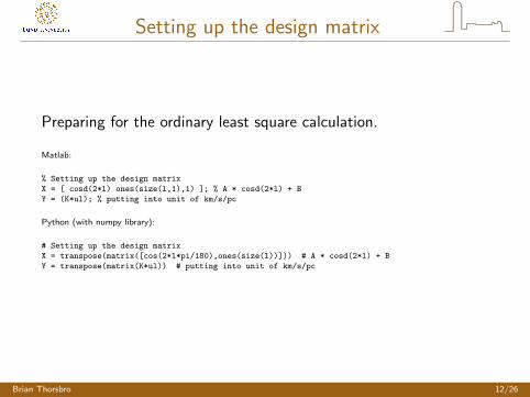
Setting up the design matrix

Preparing for the ordinary least square calculation.

Matlab:

% Setting up the design matrix

X = [ cosd(2*l) ones(size(l,1),1) ]; % A * cosd(2*l) + B

Y = (K*ul); % putting into unit of km/s/pc

Python (with numpy library):

# Setting up the design matrix

X = transpose(matrix([cos(2*l*pi/180),ones(size(l))])) # A * cosd(2*l) + B

Y = transpose(matrix(K*ul)) # putting into unit of km/s/pc


Doing the least square

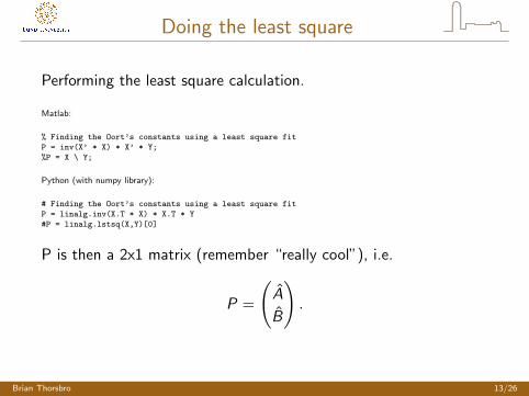
Performing the least square calculation.

Matlab:

% Finding the Oort’s constants using a least square fit

P = inv(X’ * X) * X’ * Y;

%P = X \ Y;


# Finding the Oort’s constants using a least square fit

P = linalg.inv(X.T * X) * X.T * Y

#P = linalg.lstsq(X,Y)[0]

P is then a 2x1 matrix (remember “really cool”), i.e.

P =

(A

B

).


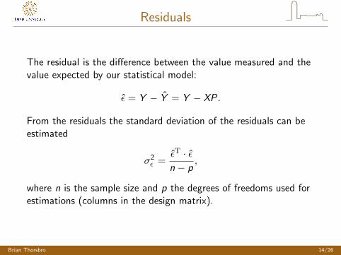
Residuals

The residual is the difference between the value measured and thevalue expected by our statistical model:

ε = Y − Y = Y − XP.

From the residuals the standard deviation of the residuals can beestimated

σ2ε =

εT · εn − p

,

where n is the sample size and p the degrees of freedoms used forestimations (columns in the design matrix).


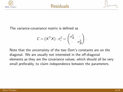
Residuals

The variance-covariance matrix is defined as

C = (XTX ) · σ2ε =

(σ2A ·· σ2

B

).

Note that the uncertainty of the two Oort’s constants are on thediagonal. We are usually not interested in the off-diagonalelements as they are the covariance values, which should all be verysmall preferably, to claim independence between the parameters.


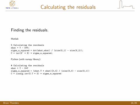
Calculating the residuals

Finding the residuals.

Matlab:

% Calculating the residuals

ehat = Y - X*P;

sigma_e_squared = dot(ehat,ehat) / (size(X,1) - size(X,2));

C = inv(X’ * X) * sigma_e_squared;


# Calculating the residuals

ehat = Y - X*P

sigma_e_squared = (ehat.T * ehat)[0,0] / (size(X,0) - size(X,1))

C = linalg.inv(X.T * X) * sigma_e_squared


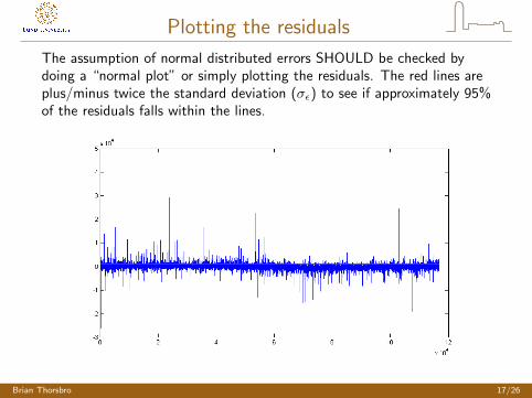
Plotting the residuals

The assumption of normal distributed errors SHOULD be checked bydoing a “normal plot” or simply plotting the residuals. The red lines areplus/minus twice the standard deviation (σε) to see if approximately 95%of the residuals falls within the lines.


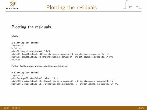
Plotting the residuals

Plotting the residuals.

Matlab:

% Plotting the errors

figure(1)

hold on

plot(1:length(ehat),ehat,’-b’)

plot([1 length(ehat)],[2*sqrt(sigma_e_squared) 2*sqrt(sigma_e_squared)],’-r’)

plot([1 length(ehat)],[-2*sqrt(sigma_e_squared) -2*sqrt(sigma_e_squared)],’-r’)

hold off

Python (with numpy and matplotlib.pyplot libraries):

# Plotting the errors

figure(1)

plot(arange(0,size(ehat)),ehat,’-b’)

plot([0 , size(ehat)-1],[2*sqrt(sigma_e_squared) , 2*sqrt(sigma_e_squared)],’-r’)

plot([0 , size(ehat)-1],[-2*sqrt(sigma_e_squared) , -2*sqrt(sigma_e_squared)],’-r’)


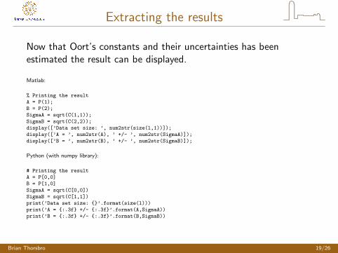
Extracting the results

Now that Oort’s constants and their uncertainties has beenestimated the result can be displayed.

Matlab:

% Printing the result

A = P(1);

B = P(2);

SigmaA = sqrt(C(1,1));

SigmaB = sqrt(C(2,2));

display([’Data set size: ’, num2str(size(l,1))]);

display([’A = ’, num2str(A), ’ +/- ’, num2str(SigmaA)]);

display([’B = ’, num2str(B), ’ +/- ’, num2str(SigmaB)]);


# Printing the result

A = P[0,0]

B = P[1,0]

SigmaA = sqrt(C[0,0])

SigmaB = sqrt(C[1,1])

print(’Data set size: {}’.format(size(l)))

print(’A = {:.3f} +/- {:.3f}’.format(A,SigmaA))

print(’B = {:.3f} +/- {:.3f}’.format(B,SigmaB))


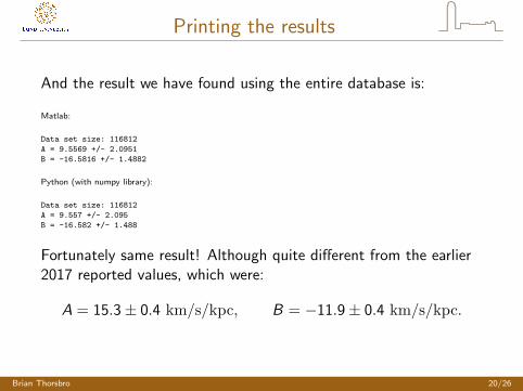
Printing the results

And the result we have found using the entire database is:

Matlab:

Data set size: 116812

A = 9.5569 +/- 2.0951

B = -16.5816 +/- 1.4882


Data set size: 116812

A = 9.557 +/- 2.095

B = -16.582 +/- 1.488

Fortunately same result! Although quite different from the earlier2017 reported values, which were:

A = 15.3± 0.4 km/s/kpc, B = −11.9± 0.4 km/s/kpc.


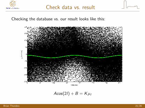
Check data vs. result

Checking the database vs. our result looks like this:

Acos(2l) + B = Kµl


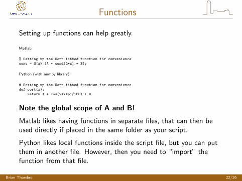
Functions

Setting up functions can help greatly.

Matlab:

% Setting up the Oort fitted function for convenience

oort = @(x) (A * cosd(2*x) + B);


# Setting up the Oort fitted function for convenience

def oort(x):

return A * cos(2*x*pi/180) + B

Note the global scope of A and B!

Matlab likes having functions in separate files, that can then beused directly if placed in the same folder as your script.

Python likes local functions inside the script file, but you can putthem in another file. However, then you need to “import” thefunction from that file.


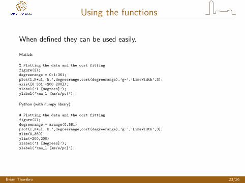
Using the functions

When defined they can be used easily.

Matlab:

% Plotting the data and the oort fitting

figure(2);

degreerange = 0:1:361;

plot(l,K*ul,’k.’,degreerange,oort(degreerange),’g-’,’LineWidth’,3);

axis([0 361 -200 200]);

xlabel(’l [degrees]’);

ylabel(’\mu_l [km/s/pc]’);


# Plotting the data and the oort fitting

figure(2);

degreerange = arange(0,361)

plot(l,K*ul,’k.’,degreerange,oort(degreerange),’g-’,’LineWidth’,3);

xlim(0,360)

ylim(-200,200)

xlabel(’l [degrees]’);

ylabel(’\mu_l [km/s/pc]’);


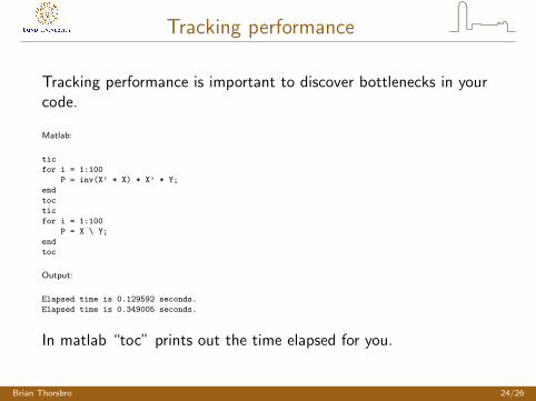
Tracking performance

Tracking performance is important to discover bottlenecks in yourcode.

Matlab:

tic

for i = 1:100

P = inv(X’ * X) * X’ * Y;

end

toc

tic

for i = 1:100

P = X \ Y;

end

toc

Output:

Elapsed time is 0.129592 seconds.

Elapsed time is 0.349005 seconds.

In matlab “toc” prints out the time elapsed for you.


Tracking performance

Tracking performance is important to discover bottlenecks in yourcode.

Python (with numpy and timit libraries):

import timeit

tic = timeit.default_timer()

for i in range(0,100):

P = linalg.inv(X.T * X) * X.T * Y

toc = timeit.default_timer()

print(toc-tic)

tic = timeit.default_timer()

for i in range(0,100):

P = linalg.lstsq(X,Y)[0]

toc = timeit.default_timer()

print(toc-tic)

Output:

0.12253564078859469

0.18159674188904162

In python the time returns seconds passed and you can print outthe difference manually.


The End

Questions?


Documents

Introduction to programming with Matlab/Python Lecture 2 2/compintro-lecture2.pdf · observing nearby stars one could say something about the rotation curve of ... Performing the