Introduction to Probability Theory · Introduction to Probability Theory Daria Lavrentev University of Freiburg October 16, 2014 1/36. BasicsDiscreate Random VariablesContinuous Random

Basics Discreate Random Variables Continuous Random Variables Important Discrete Distributions Important Continuous Distributions Useful Properties Sample Distribution

Introduction to Probability Theory

Daria Lavrentev

University of Freiburg

October 16, 2014

1 / 36


Main reference:Mathematical Statistics with Applications by John E. Freund.Available in the seminar library S1/1427

2 / 36


1 Basics

2 Discreate Random Variables

3 Continuous Random Variables

4 Important Discrete Distributions

5 Important Continuous Distributions

6 Useful Properties

7 Sample Distribution

3 / 36


Basics

We would often be interested in studying a phenomenon, wherethere is an uncertainty about the outcome. A random phenomenonis also refered to as an experiment.

• A set of all possible outcomes of an experiment is called thesample space and is denoted by Ω (or sometimes S).

One can be interested in results which are not given directly by aspecific element of a sample spase.

• An event is a subset of the sumple space.

Example

Rolling a dice.The sample space is:1, 2, 3, 4, 5, 6 .1, 2 represents an event that rolling a dice resulted in 1 or 2.

4 / 36


Basics

We denote events by capital letters.The probability of an event A is denoted by Prob(A) (or often byP(A)).Some useful properties:

• P(Ω) = 1

• P(A′) = 1− P(A)

• P(∅) = 0

• Given A and B two events, such that A ⊆ B, it holds thatP(A) ≤ P(B).

• P(A) ∈ [0, 1]

• If A and B are mutualy exclusive events (A ∩ B = ∅), thenProb(A ∪ B) = P(A) + P(B)

5 / 36


Basics

The conditional probability of event A given event B is definedas:

P(A|B) =P(A ∩ B)

P(B)

Two events A and B are said to be independent if and only if

P(A ∩ B) = P(A) · P(B)

6 / 36


Random Variable

A random variable is a function that associates a uniquenumerical value with outcome of a random phenomenon/anexperiment.One distinguishes between two types of random variables: discreteand continuous.

• Discrete random variable is a random variable that canobtain a finite, or countable infinite number of values.Note that since the number of values is countable, we candenote them by :x1, x2, ..., xn, ...

• Continuous random variable is a random variable that canobtain any value in R.

Remark: the definition of the continious r.v. is often different.

7 / 36


Random Variable

Examples

• Rolling a dice.

• Number of mistakes on a page of a book.

• Waiting time in a queue at a service point.

• Weight of a child of a certain age.

• Stock price.

8 / 36


p.d.f and c.d.f

• The probability distribution function of a discrete randomvariable, f (x) describes the probability of the variable toobtain a certain value x ,

f (x) = Prob(X = x)

• Cumulative destribution function is defined as theprobability of the given variable X to obtain a value equal orsmaller than x ,

F (x) = Prob(X ≤ x) =∑xi≤x

f (xi )

9 / 36


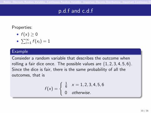
p.d.f and c.d.f

Properties:

• f (x) ≥ 0

•∑∞

i=1 f (xi ) = 1

Example

Consieder a random variable that describes the outcome whenrolling a fair dice once. The possible values are 1, 2, 3, 4, 5, 6.Since the dice is fair, there is the same probability of all theoutcomes, that is

f (x) =

16 x = 1, 2, 3, 4, 5, 6

0 otherwise.

10 / 36


p.d.f and c.d.f

Example

The cumulative distribution finction in this case is:

F (x) =

0 x < 1

16 , x ∈ [1, 2)

26 , x ∈ [2, 3)

36 , x ∈ [3, 4)

46 , x ∈ [4, 5)

56 , x ∈ [5, 6)

1 x ≥ 6

11 / 36


Expected Value

For a discrete random variable X with density function f (x) theexpected value is defined as:

E(X ) = µX =∞∑i=1

xi · f (xi )

The following terms often refer to the same thing!

Expected Value = Mean = Expectations = Average

Example

Continuing the previous example,

E(X ) =∑∞

i=1 xi · f (xi ) =

= 1 · 16 + 2 · 16 + 3 · 16 + 4 · 16 + 5 · 16 + 6 · 16 + 7 · 0 + ...

= 216 = 3.5

12 / 36


Variation and Standard Deviation

The variance of a discrete random variable X is defined as:

Var(X ) = σ2X =∞∑i=1

(xi − µX )2 · f (xi ).

Standard deviation is: σX =√

Var(X )

Example

For the example discussed above we have:

Var(X ) =∑∞

i=1(xi − µX )2 · f (xi ) =

(1− 3.5)2 · 16 + (2− 3.5)2 · 16 + (3− 3.5)2 · 16 + (4− 3.5)2 · 16+

+(5− 3.5)2 · 16 + (6− 3.5)2 · 16 + (7− 3.5)2 · 0 + ... = 17.56

=⇒ σ ≈ 1.7078

13 / 36


Moment of Order r

For a random variable X , it’s moment of order r is defined as:

M rX = E(X r ) =

∞∑i=1

x ri · f (xi ),

sometimes one talks about the central moment, also refered to asthe moment about the mean, that is:

M rX = E[(X − µX )r ] =

∞∑i=1

(xi − µX )r · f (xi )

Example

σ2x is the central moment of X .

14 / 36


p.d.f and c.d.f

• A function f (x) defined on the set of real numbers is called aprobability density function of a continious random variableX if and only if

Prob(a ≤ X ≤ b) =

∫ b

af (x)dx

for any a, b ∈ R, such that a ≤ b.

• Cumulative destribution function is defined as theprobability of the given variable X to obtain a value equal orsmaller than x ,

F (x) = Prob(X ≤ x) =

∫ x

−∞f (z)dz

15 / 36


p.d.f and c.d.f

16 / 36


p.d.f and c.d.f

• Note the difference to the discrete case!

• A function f (x) can serve as a probability density functiononly if it has the following properties:

1 f (x) ≥ 0 ∀x ∈ R,

2∫∞−∞ f (x)dx = 1.

• P(a ≤ X ≤ b) = F (b)− F (a)

• If c.d.f. of a random variable X is differentiable, then

f (x) =dF (x)

dx.

17 / 36


p.d.f and c.d.f

Example

A random variable X follows the exponential distribution withparameter λ if it has the folowing c.d.f. and p.d.f.

F (x) =

1− e−λx x ≥ 00 x < 0

and

f (x) =

λe−λx x ≥ 00 x < 0

We denote X ∼ exp(λ)

18 / 36


Expected Value

• For a continuous random variable X with density functionf (x) the expected value is defined as:

E(X ) = µX =

∫ ∞−∞

x · f (x)dx

• Let Y be a randon variable defined by Y = g(X ), where g(∗)is a real function of single variable. The expected value of Yis:

E(Y ) = E(g(X )) =

∫ ∞−∞

g(x) · f (x)dx

19 / 36


Variation and Standard Deviation

The variance of a continuous random variable is:

Var(X ) = σ2 = E((X − µX )2)

Note that

Var(X ) = E((X − µX )2) =

∫ ∞−∞

(x − µX )2 · f (x)dx =

=

∫ ∞−∞

(x2 − 2xµX + µ2X ) · f (x)dx =

=

∫ ∞−∞

x2 · f (x)dx −∫ ∞−∞

2xµX · f (x)dx +

∫ ∞−∞

µ2X · f (x)dx =

= E(X 2)− µ2X

20 / 36


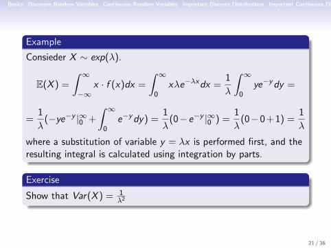
Example

Consieder X ∼ exp(λ).

E(X ) =

∫ ∞−∞

x · f (x)dx =

∫ ∞0

xλe−λxdx =1

λ

∫ ∞0

ye−ydy =

=1

λ(−ye−y |∞0 +

∫ ∞0

e−ydy) =1

λ(0− e−y |∞0 ) =

1

λ(0−0 + 1) =

1

λ

where a substitution of variable y = λx is performed first, and theresulting integral is calculated using integration by parts.

Exercise

Show that Var(X ) = 1λ2

21 / 36


Moment of Order r

Similar to the discrete case, a moment of order r is defined as:

M rX = E(X r )

The moment about the mean is:

M rX = E[(X − µX )r ]

Example

σ2x is the second moment around the mean.

22 / 36


Important Discrete Distributions

• Bernoulli distributionA single toss of a coin with probability p of obtaining heads.Let X be a random variable obtaining 1 if the result is headsand 0 if the result is tails.

f (x) =

p x = 11− p x = 0

E(X ) = p,

Var(X ) = p(1− p)

23 / 36


Important Discrete Distributions

• Binomial distributionRepresents the number of successes in a sequence of nindependent yes/no experiments, each of which yieldssuccess(yes) with probability p.

f (x) =( n

x

)px(1− p)n−x , x = 0, 1, 2, ...

E(X ) = np,

Var(X ) = np(1− p)

24 / 36


Important Continuous Distributions

• Uniform distributionX is uniform distributed on interval (a, b) it it’s densityfunction is:

f (x) =

1

b−a a < x < b

0 otherwise,

E(X ) =a + b

2,

Var(x) =(b − a)2

12

25 / 36


Important Continuous Distributions

• Normal distribution with mean µ and variance σ2

f (x) =1√2πσ

e−12(x−µ)2

σ2

If σ2 = 1 and µ = 0 we say that the distribution is a standardnormal dositribution.

• Exponential distribution

26 / 36


Joint Probability and Density

• Given two discrete r.v. X and Y , the function given by

f (x , y) = Prob(X = x ,Y = y)

is called the joint probability distribution function of X andY .

• A bivariate function f (x , y) is called a joint probabilitydensity function of the continuous r.v. X and Y if and only if

Prob[(X ,Y ) ∈ A] =

∫ ∫Af (x , y)dxdy

for any region A in the xy plane.

27 / 36


Joint Distribution

• Given two discrete r.v. X and Y , the function

F (x , y) = Prob(X ≤ x ,Y ≤ y) =∑s≤x

∑t≤y

f (s, t)

where (x , y) ∈ R2 and f (s, t) is the joint probabilitydensity, is the joint distribution function, or the jointcumulative distribution, of X and Y .

• Given two continuous r.v. X and Y , the function

F (x , y) = Prob(X ≤ x ,Y ≤ y) =

∫ x

−∞

∫ y

−∞f (s, t)dsdt

where (x , y) ∈ R2 and f (s, t) is the joint probability density, iscalled the joint distribution function of X and Y .

28 / 36


Marginal Distribution and Density.

• Given two discrete r.v. X and Y with joint probabilitydistribution f (x , y), the function

g(x) =∑y

f (x , y)

is called the marginal distribution of X .In a similar way, h(y) =

∑x f (x , y) is the marginal

distribution of Y .

• Given two continuous r.v. X and Y ,with joint dinsity f (x , y),the function

g(x) =

∫ ∞−∞

f (x , y)dy

is called the marginal density of X .In a similar way, h(y) =

∫∞−∞ f (x , y)dy is the marginal density

of Y .29 / 36


Independent Random Variables

Given two random variables X1 and X2 with jointdistribution/density function f (x1, x2) and distribution/densityfunctions f1(x1) and f2(x2), we say that the variables X1 and X2

are independent if and only if

f (x1, x2) = f1(x1) · f2(x2).

If the above does not call, we say that the two random variabllesare dependent or correlated.

30 / 36


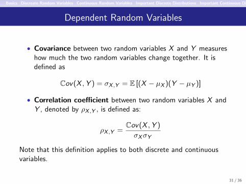
Dependent Random Variables

• Covariance between two random variables X and Y measureshow much the two random variables change together. It isdefined as

Cov(X ,Y ) = σX ,Y = E [(X − µX )(Y − µY )]

• Correlation coefficient between two random variables X andY , denoted by ρX ,Y , is defined as:

ρX ,Y =Cov(X ,Y )

σXσY

Note that this definition applies to both discrete and continuousvariables.

31 / 36


Useful Properties

• E[αX ] = αE[X ]

• E[X + Y ] = E[X ] + E[Y ]

• E[X 2] = Var [X ] + E2[X ]

• If X and Y are independent r.v. then E[XY ] = E[X ]E[Y ]

• Var [αX ] = α2Var [X ]

• If X and Y are independent r.v. thenVar [aX + bY ] = a2Var [X ] + b2Var [Y ]

• If X and Y are dependent r.v. thenVar [aX + bY ] = a2Var [X ] + b2Var [Y ] + 2abCov(X ,Y )

where α, a, b ∈ R, X and Y are random variables.

32 / 36


Sample Mean, Variance and Covariance

Given a random sample x1, x2, x3, ..., xN we can find the mean as

X =

∑Ni=1 xiN

The sample variance is

σ2 =

∑Ni=1(xi − X )2

N

The sample covariance of two random samples x1, x2, x3, ..., xN andy1, y2, y3, ..., yN is

Cov(X ,Y ) =

∑Ni=1(xi − X )(yi − Y )

N

Remark: for variance and covariance, sometimes N will be replacedwith N − 1.

33 / 36


Var-Covariance Matrix

Given N observations for each of M random varibles,which aregiven in a matrix form X , where each column of the matrix givesthe N observations of a single variable, the variance-covariancematrix is the following matrix,

Σ =(σij)i ,j=1...M

, where σij = Cov(Xi ,Xj)

We note that this matrix is symetric and that the diagonalelements are the sample variance of the variables.

34 / 36


Var-Covariance Matrix

Important Example

Assuming that the variavles represented by the matrix X have asample variance of zero, the var-covar. matrix can be calculated as

1

MX>X

35 / 36


Important Application

Consider an economy with two periods, today (t = 0) andtomorrow (t=1). There is uncertainty about the economy statetomorrow. There are s possible states. The probabilities of eachstate to occur is given by (π1, π2, ..., πs). In addition we know thatthe state contingent consumption of an agent in this economy isgiven by (c1, c2, ..., cs) and that the agent’s utility of consuming cunits is equal to u(c) =

√c.

The expected utility of the agent in this economy is:

E (u(c)) =s∑

i=1

πiu(ci ) =s∑

i=1

πi√ci

36 / 36

Documents

Introduction to Probability Theory · Introduction to Probability Theory Daria Lavrentev University of Freiburg October 16, 2014 1/36. BasicsDiscreate Random VariablesContinuous Random