Introduction to plm - Welcome to the University of Bayreuthftp.uni-bayreuth.de/math/statlib/R/CRAN/doc/vignettes/plm/plmEN.pdf · Introduction to plm Yves Croissant & Giovanni Millo

Introduction to plm

Yves Croissant & Giovanni Millo

May 14, 2007

1 Introduction

The aim of package plm is to provide an easy way to estimate panel models.Some panel models may be estimated with package nlme (non–linear mixedeffect models), but not in an intuitive way for an econometrician. plm providesmethods to read panel data, to estimate a wide range of models and to makesome tests. This library is loaded using :

> library(plm)

This document illustrates the features of plm, using data available in packageEcdat.

> library(Ecdat)

These data are used in Baltagi (2001).

2 Reading data

With plm, data are stored in an object of class pdata.frame, which is a data.framewith additional attributes describing the structure of the data set. A pdata.framemay be created from an ordinary data.frame using the pdata.frame functionor from a text file using the pread.table function.

2.1 Reading the data from a data.frame

We illustrate the use of the pdata.frame function with the Produc data :

> data(Produc)

> pdata.frame(Produc, "state", "year", "pprod")

The pdata.frame function has 4 arguments :

the name of the data.frame,

id : the individual index,

1

time : the time index,

name : the name under which the pdata.frame will be stored.

Observations are assumed to be sorted by individuals first, and by period.The third argument is optional, if NULL a new variable called time is added.The fourth argument is also optional, if NULL the pdata.frame is stored underthe same name as the data.frame.

> data(Hedonic)

> pdata.frame(Hedonic, "townid")

In case of a balanced panel, the id may be the number of individuals. Inthis case, two new variables (called id and time) are added.

> data(Wages)

> pdata.frame(Wages, 595)

A description of the data is obtained using the summary method :

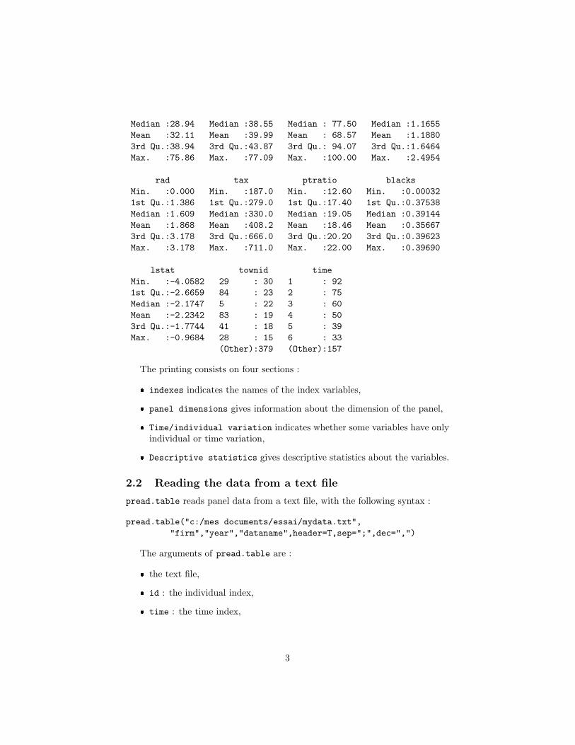
> summary(Hedonic)

___________________________________________________________________________________________________________________ Indexes ____________________________________Individual index : townidTime index : time_______________________________________________________________________________________________________________ Panel Dimensions _______________________________Unbalanced PanelNumber of Individuals : 92Number of Time Observations : from 1 to 30Total Number of Observations : 506__________________________________________________________________________________________________________ Time/Individual Variation ___________________________no time variation : zn indus rad tax ptratio____________________________________________________________________________________________________________ Descriptive Statistics ____________________________

mv crim zn indus chasMin. : 8.517 Min. : 0.00632 Min. : 0.00 Min. : 0.46 no :4711st Qu.: 9.742 1st Qu.: 0.08205 1st Qu.: 0.00 1st Qu.: 5.19 yes: 35Median : 9.962 Median : 0.25651 Median : 0.00 Median : 9.69Mean : 9.942 Mean : 3.61352 Mean : 11.36 Mean :11.143rd Qu.:10.127 3rd Qu.: 3.67708 3rd Qu.: 12.50 3rd Qu.:18.10Max. :10.820 Max. :88.97620 Max. :100.00 Max. :27.74

nox rm age disMin. :14.82 Min. :12.68 Min. : 2.90 Min. :0.12191st Qu.:20.16 1st Qu.:34.64 1st Qu.: 45.02 1st Qu.:0.7420

2

Median :28.94 Median :38.55 Median : 77.50 Median :1.1655Mean :32.11 Mean :39.99 Mean : 68.57 Mean :1.18803rd Qu.:38.94 3rd Qu.:43.87 3rd Qu.: 94.07 3rd Qu.:1.6464Max. :75.86 Max. :77.09 Max. :100.00 Max. :2.4954

rad tax ptratio blacksMin. :0.000 Min. :187.0 Min. :12.60 Min. :0.000321st Qu.:1.386 1st Qu.:279.0 1st Qu.:17.40 1st Qu.:0.37538Median :1.609 Median :330.0 Median :19.05 Median :0.39144Mean :1.868 Mean :408.2 Mean :18.46 Mean :0.356673rd Qu.:3.178 3rd Qu.:666.0 3rd Qu.:20.20 3rd Qu.:0.39623Max. :3.178 Max. :711.0 Max. :22.00 Max. :0.39690

lstat townid timeMin. :-4.0582 29 : 30 1 : 921st Qu.:-2.6659 84 : 23 2 : 75Median :-2.1747 5 : 22 3 : 60Mean :-2.2342 83 : 19 4 : 503rd Qu.:-1.7744 41 : 18 5 : 39Max. :-0.9684 28 : 15 6 : 33

(Other):379 (Other):157

The printing consists on four sections :

indexes indicates the names of the index variables,

panel dimensions gives information about the dimension of the panel,

Time/individual variation indicates whether some variables have onlyindividual or time variation,

Descriptive statistics gives descriptive statistics about the variables.

2.2 Reading the data from a text file

pread.table reads panel data from a text file, with the following syntax :

pread.table("c:/mes documents/essai/mydata.txt","firm","year","dataname",header=T,sep=";",dec=",")

The arguments of pread.table are :

the text file,

id : the individual index,

time : the time index,

3

name : the name under which the pdata.frame will be stored (if NULL,the name of the pdata.frame is the name of the file without the path andthe extension),

further arguments that will be passed to read.table.

3 Model estimation

plm provides four functions for estimation :

plm : estimation of the basic panel models, i.e. within, between andrandom effect models. Models are estimated using the lm function totransformed data,

pvcm : estimation of models with variable coefficients,

pgmm : estimation of general method of moments models,

pggls : estimation of general feasible generalized least squares models.

All these functions share the same 4 first arguments :

formula : the symbolic description of the model to be estimated,

data : the pdata.frame containing the data,

effect : the kind of effects to include in the model, i.e. individual effects,time effects or both,

model : the kind of model to be estimated, most of the time a model withfixed effects or a model with random effects.

The results of this four functions are stored in an object which class hasthe same name of the function. They all inherit from class panelmodel. Apanelmodel object contains : coefficients, residuals, fitted.values, vcov,df.residual and call.

Functions that extract these elements and to print the object are provided.

3.1 Estimation of the basic models with plm

There are two ways to use plm : the first one is to estimate a list of models (thedefault behavior), the second to estimate just one model. In the first case, theestimated models are :

the fixed effects model (within),

the pooling model (pooling),

the between model (between),

4

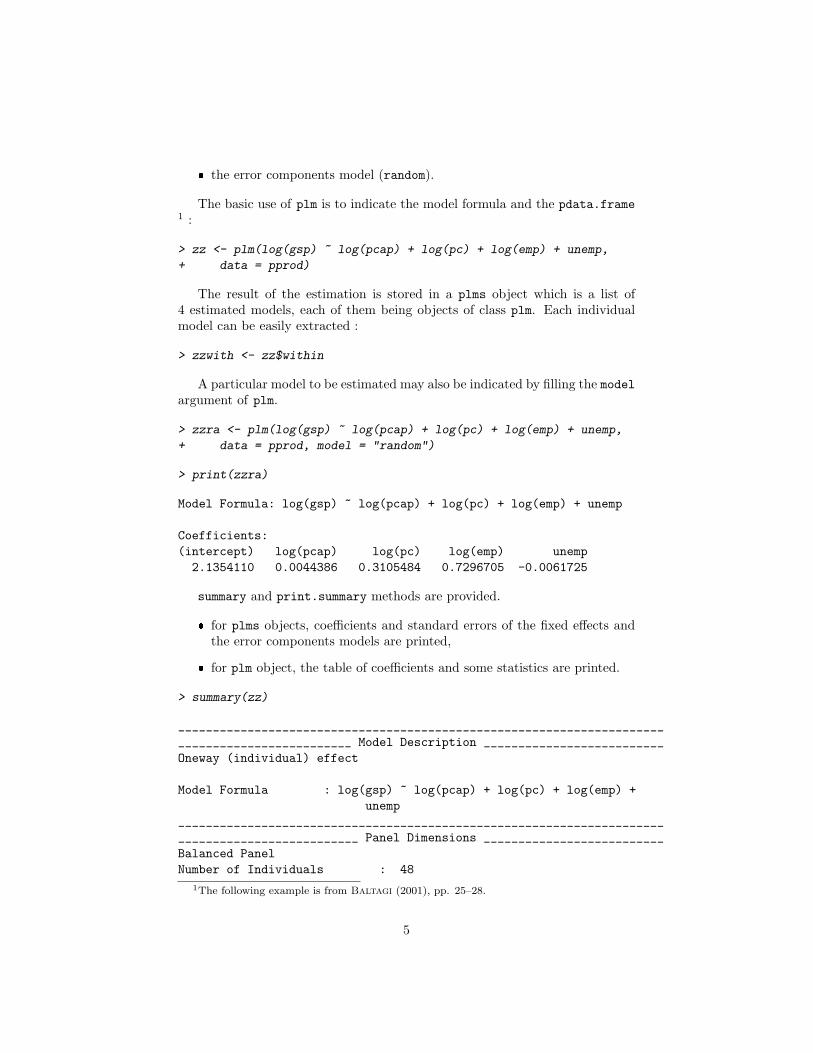
the error components model (random).

The basic use of plm is to indicate the model formula and the pdata.frame1 :

> zz <- plm(log(gsp) ~ log(pcap) + log(pc) + log(emp) + unemp,

+ data = pprod)

The result of the estimation is stored in a plms object which is a list of4 estimated models, each of them being objects of class plm. Each individualmodel can be easily extracted :

> zzwith <- zz$within

A particular model to be estimated may also be indicated by filling the modelargument of plm.

> zzra <- plm(log(gsp) ~ log(pcap) + log(pc) + log(emp) + unemp,

+ data = pprod, model = "random")

> print(zzra)

Model Formula: log(gsp) ~ log(pcap) + log(pc) + log(emp) + unemp

Coefficients:(intercept) log(pcap) log(pc) log(emp) unemp2.1354110 0.0044386 0.3105484 0.7296705 -0.0061725

summary and print.summary methods are provided.

for plms objects, coefficients and standard errors of the fixed effects andthe error components models are printed,

for plm object, the table of coefficients and some statistics are printed.

> summary(zz)

_______________________________________________________________________________________________ Model Description __________________________Oneway (individual) effect

Model Formula : log(gsp) ~ log(pcap) + log(pc) + log(emp) +unemp

________________________________________________________________________________________________ Panel Dimensions __________________________Balanced PanelNumber of Individuals : 48

1The following example is from Baltagi (2001), pp. 25–28.

5

Number of Time Observations : 17Total Number of Observations : 816__________________________________________________________________________________________________ Coefficients ____________________________

within wse random rse(intercept) . . 2.13541100 0.1335log(pcap) -0.02614965 0.02813133 0.00443859 0.0234log(pc) 0.29200693 0.02436591 0.31054843 0.0198log(emp) 0.76815947 0.02918878 0.72967053 0.0249unemp -0.00529774 0.00095906 -0.00617247 0.0009_____________________________________________________________________________________________________ Tests ________________________________Hausman Test : chi2(4) = 190.8961 (p.value=0)F Test : F(47,764) = 75.8204 (p.value=0)Lagrange Multiplier Test : chi2(1) = 4134.961 (p.value=0)______________________________________________________________________

> summary(zzra)

_______________________________________________________________________________________________ Model Description __________________________Oneway (individual) effectRandom Effect Model (Swamy-Arora's transformation)Model Formula : log(gsp) ~ log(pcap) + log(pc) + log(emp) +

unemp________________________________________________________________________________________________ Panel Dimensions __________________________Balanced PanelNumber of Individuals : 48Number of Time Observations : 17Total Number of Observations : 816____________________________________________________________________________________________________ Effects _______________________________

var std.dev shareidiosyncratic 0.0014544 0.0381371 0.1754individual 0.0068377 0.0826905 0.8246theta : 0.88884___________________________________________________________________________________________________ Residuals ______________________________

Min. 1st Qu. Median Mean 3rd Qu. Max.-1.07e-01 -2.46e-02 -2.37e-03 -9.93e-19 2.17e-02 2.00e-01__________________________________________________________________________________________________ Coefficients ____________________________

Estimate Std. Error z-value Pr(>|z|)(intercept) 2.13541100 0.13346149 16.0002 < 2.2e-16 ***log(pcap) 0.00443859 0.02341732 0.1895 0.8497

6

log(pc) 0.31054843 0.01980475 15.6805 < 2.2e-16 ***log(emp) 0.72967053 0.02492022 29.2803 < 2.2e-16 ***unemp -0.00617247 0.00090728 -6.8033 1.023e-11 ***---Signif. codes: 0 ‘***’ 0.001 ‘**’ 0.01 ‘*’ 0.05 ‘.’ 0.1 ‘ ’ 1_______________________________________________________________________________________________ Overall Statistics _________________________Total Sum of Squares : 29.209Residual Sum of Squares : 1.1879Rsq : 0.95933F : 4782.77P(F>0) : 8.76231e-08______________________________________________________________________

For a random model, the summary method gives information about the vari-ance of the components of the errors.

plm objects can be updated using the update method :

> zzwithmod <- update(zzwith, . ~ . - unemp - log(emp) + emp)

> zzmod <- update(zz, . ~ . - unemp - log(emp) + emp)

> summary(zzwithmod)

_______________________________________________________________________________________________ Model Description __________________________Oneway (individual) effect

Model Formula : log(gsp) ~ log(pcap) + log(pc) + emp________________________________________________________________________________________________ Panel Dimensions __________________________Balanced PanelNumber of Individuals : 48Number of Time Observations : 17Total Number of Observations : 816__________________________________________________________________________________________________ Coefficients ____________________________

within wse random rse(intercept) . . 7.1982e-01 0.1846log(pcap) 1.7888e-01 3.9471e-02 3.4357e-01 0.0322log(pc) 6.9975e-01 2.8280e-02 6.0369e-01 0.0256emp 3.7909e-05 8.5192e-06 5.0924e-05 8.218e-06_____________________________________________________________________________________________________ Tests ________________________________Hausman Test : chi2(3) = 32.23348 (p.value=4.672804e-07)F Test : F(47,765) = 101.9109 (p.value=0)Lagrange Multiplier Test : chi2(1) = 4355.292 (p.value=0)______________________________________________________________________

7

Fixed effects may be extracted easily from a plms or a plm object using FE :

> FE(zzmod)[1:10]

ALABAMA ARIZONA ARKANSAS CALIFORNIA COLORADO CONNECTICUT1.171753 1.306239 1.187700 1.619198 1.458215 1.706034DELAWARE FLORIDA GEORGIA IDAHO1.203575 1.556497 1.446017 1.100205

The FE function returns an object of class FE. A summary method is pro-vided, which prints the effects (in deviation from the overall intercept), theirstandard errors and the test of equality to the overall intercept.

> summary(FE(zzmod))[1:10, ]

FE std.error t-value p-valueALABAMA -0.15044698 0.2142832 -0.70209405 0.48262051ARIZONA -0.01596112 0.2115486 -0.07544893 0.93985753ARKANSAS -0.13449962 0.2009406 -0.66935022 0.50327210CALIFORNIA 0.29699815 0.2450846 1.21181889 0.22558172COLORADO 0.13601482 0.2109386 0.64480772 0.51905180CONNECTICUT 0.38383408 0.2155489 1.78072876 0.07495677DELAWARE -0.11862549 0.1892258 -0.62689921 0.53072531FLORIDA 0.23429687 0.2269427 1.03240541 0.30188224GEORGIA 0.12381708 0.2193786 0.56439904 0.57248259IDAHO -0.22199517 0.1852999 -1.19803151 0.23090475

3.2 More advanced use of plm

3.2.1 Options for the random effect model

The random effect model is obtained as a linear estimation on quasi–differentiateddata. The parameter of this transformation is obtained using preliminary es-timations. Four estimators of this parameter are available, depending on thevalue of the argument random.method :

swar : from Swamy and Arora (1972), the default value,

walhus : from Wallace and Hussain (1969),

amemiya : from Amemiyia (1971),

nerlove : from Nerlove (1971).

For exemple, to use the amemiya estimator :

> zzra <- plm(log(gsp) ~ log(pcap) + log(pc) + log(emp) + unemp,

+ data = pprod, model = "random", random.method = "amemiya")

8

3.2.2 Choosing the effects

The default behavior of plm is to introduce individual effects. Using the effectargument, one may also introduce :

time effects (effect="time"),

individual and time effects (effect="twoways").

For example, to estimate a two–ways effect model for the Grunfeld data :

> data(Grunfeld)

> pdata.frame(Grunfeld, "firm", "year")

> z <- plm(inv ~ value + capital, data = Grunfeld, effect = "twoways",

+ random.method = "amemiya")

> summary(z$random)

_______________________________________________________________________________________________ Model Description __________________________Twoways effectsRandom Effect Model (Amemiya's transformation)Model Formula : inv ~ value + capital________________________________________________________________________________________________ Panel Dimensions __________________________Balanced PanelNumber of Individuals : 10Number of Time Observations : 20Total Number of Observations : 200____________________________________________________________________________________________________ Effects _______________________________

var std.dev shareidiosyncratic 2644.135 51.421 0.2359individual 8294.716 91.075 0.7400time 270.529 16.448 0.0241theta : 0.87475 (id) 0.29695 (time) 0.29595 (total)___________________________________________________________________________________________________ Residuals ______________________________

Min. 1st Qu. Median Mean 3rd Qu. Max.-1.76e+02 -1.80e+01 3.02e+00 -3.56e-16 1.80e+01 2.33e+02__________________________________________________________________________________________________ Coefficients ____________________________

Estimate Std. Error z-value Pr(>|z|)(intercept) -64.351811 31.183651 -2.0636 0.03905 *value 0.111593 0.011028 10.1192 < 2e-16 ***capital 0.324625 0.018850 17.2214 < 2e-16 ***---Signif. codes: 0 ‘***’ 0.001 ‘**’ 0.01 ‘*’ 0.05 ‘.’ 0.1 ‘ ’ 1

9

_______________________________________________________________________________________________ Overall Statistics _________________________Total Sum of Squares : 2038000Residual Sum of Squares : 514120Rsq : 0.74774F : 291.965P(F>0) : 0.00341914______________________________________________________________________

In the “effects” section of the result is printed now the variance of the threeelements of the error term and the three parameters used in the transformation.

The two–ways effect model is for the moment only available for balancedpanels.

3.2.3 Hausman–Taylor’s model

Hausman–Taylor’s model may be estimated with plm by equating the modelargument to "ht" and filling the second argument instruments with a formulaindicating the variables used as instruments.

> data(Wages)

> pdata.frame(Wages, 595)

> form = lwage ~ wks + south + smsa + married + exp + I(exp^2) +

+ bluecol + ind + union + sex + black + ed

> ht = plm(form, data = Wages, instruments = ~sex + black + bluecol +

+ south + smsa + ind, model = "ht")

> summary(ht)

_______________________________________________________________________________________________ Model Description __________________________Oneway (individual) effectHausman-Taylor ModelModel Formula : lwage ~ wks + south + smsa + married +

exp + I(exp^2) + bluecol + ind +union + sex + black + ed

Instrumental Variables : ~sex + black + bluecol + south + smsa +ind

Time--Varying Variablesexogenous variables : bluecolyes,southyes,smsayes,indendogenous variables : wks,marriedyes,exp,I(exp^2),unionyes

Time--Invariant Variablesexogenous variables : sexmale,blackyesendogenous variables : ed

________________________________________________________________________________________________ Panel Dimensions __________________________Balanced PanelNumber of Individuals : 595

10

Number of Time Observations : 7Total Number of Observations : 4165____________________________________________________________________________________________________ Effects _______________________________


Min. 1st Qu. Median Mean 3rd Qu. Max.-1.92e+00 -7.07e-02 6.57e-03 -2.46e-17 7.97e-02 2.03e+00__________________________________________________________________________________________________ Coefficients ____________________________

Estimate Std. Error z-value Pr(>|z|)(intercept) 2.7818e+00 3.0765e-01 9.0422 < 2.2e-16 ***wks 8.3740e-04 5.9973e-04 1.3963 0.16263southyes 7.4398e-03 3.1955e-02 0.2328 0.81590smsayes -4.1833e-02 1.8958e-02 -2.2066 0.02734 *marriedyes -2.9851e-02 1.8980e-02 -1.5728 0.11578exp 1.1313e-01 2.4710e-03 45.7851 < 2.2e-16 ***I(exp^2) -4.1886e-04 5.4598e-05 -7.6718 1.688e-14 ***bluecolyes -2.0705e-02 1.3781e-02 -1.5024 0.13299ind 1.3604e-02 1.5237e-02 0.8928 0.37196unionyes 3.2771e-02 1.4908e-02 2.1982 0.02794 *sexmale 1.3092e-01 1.2666e-01 1.0337 0.30129blackyes -2.8575e-01 1.5570e-01 -1.8352 0.06647 .ed 1.3794e-01 2.1248e-02 6.4919 8.474e-11 ***---Signif. codes: 0 ‘***’ 0.001 ‘**’ 0.01 ‘*’ 0.05 ‘.’ 0.1 ‘ ’ 1_______________________________________________________________________________________________ Overall Statistics _________________________Total Sum of Squares : 243.04Residual Sum of Squares : 95.947Rsq : 0.60522F : 489.524P(F>0) : 3.33067e-16______________________________________________________________________

3.2.4 Instrumental variables estimation

One or all of the models may be estimated using instrumental variables byindicating the list of the instrumental variables. This can be done using one ofthe two following techniques :

specifying the total list of instruments (using the instruments argument

11

of plm),

specifying, on the one hand the external instruments in the argumentinstrument and on the other hand the variables of the model that areassumed to be endogenous in the argument endog.

The instrumental variables estimator used may be indicated with the inst.methodargument :

bvk, from Balestra and Varadharajan–Krishnakumar (1987), thedefault value,

baltagi, from Baltagi (1981).

We illustrate instrumental variables estimation with the Crime data2. Thesame estimation is done using the first syntax (cr1) and the second (cr2). Theprbarr and polpc variables are assumed to be endogenous and there are twoexternal instruments taxpc and mix :

> data(Crime)

> pdata.frame(Crime, "county", "year")

> form = log(crmrte) ~ log(prbarr) + log(polpc) + log(prbconv) +

+ log(prbpris) + log(avgsen) + log(density) + log(wcon) + log(wtuc) +

+ log(wtrd) + log(wfir) + log(wser) + log(wmfg) + log(wfed) +

+ log(wsta) + log(wloc) + log(pctymle) + log(pctmin) + region +

+ smsa + year

> inst = ~log(prbconv) + log(prbpris) + log(avgsen) + log(density) +

+ log(wcon) + log(wtuc) + log(wtrd) + log(wfir) + log(wser) +

+ log(wmfg) + log(wfed) + log(wsta) + log(wloc) + log(pctymle) +

+ log(pctmin) + region + smsa + log(taxpc) + log(mix) + year

> inst2 = ~log(taxpc) + log(mix)

> endog = ~log(prbarr) + log(polpc)

> cr = plm(form, data = Crime)

> cr1 = plm(form, data = Crime, instruments = inst)

> cr2 = plm(form, data = Crime, instruments = inst2, endog = endog)

> summary(cr2$random)

_______________________________________________________________________________________________ Model Description __________________________Oneway (individual) effectRandom Effect Model (Swamy-Arora's transformation)Instrumental variable estimation (Balestra-Varadharajan-Krishnakumar's transformation)Model Formula : log(crmrte) ~ log(prbarr) + log(polpc) +

log(prbconv) + log(prbpris) +log(avgsen) + log(density) + log(wcon) +log(wtuc) + log(wtrd) + log(wfir) +

2See Baltagi (2001), pp.119–120.

12

log(wser) + log(wmfg) + log(wfed) +log(wsta) + log(wloc) + log(pctymle) +log(pctmin) + region + smsa +year

Endogenous Variables : ~log(prbarr) + log(polpc)Instrumental Variables : ~log(taxpc) + log(mix)________________________________________________________________________________________________ Panel Dimensions __________________________Balanced PanelNumber of Individuals : 90Number of Time Observations : 7Total Number of Observations : 630____________________________________________________________________________________________________ Effects _______________________________


Min. 1st Qu. Median Mean 3rd Qu. Max.-5.02e+00 -4.76e-01 2.73e-02 7.11e-16 5.26e-01 3.19e+00__________________________________________________________________________________________________ Coefficients ____________________________

Estimate Std. Error z-value Pr(>|z|)(intercept) -0.4538241 1.7029840 -0.2665 0.789864log(prbarr) -0.4141200 0.2210540 -1.8734 0.061015 .log(polpc) 0.5049285 0.2277811 2.2167 0.026642 *log(prbconv) -0.3432383 0.1324679 -2.5911 0.009567 **log(prbpris) -0.1900437 0.0733420 -2.5912 0.009564 **log(avgsen) -0.0064374 0.0289406 -0.2224 0.823977log(density) 0.4343519 0.0711528 6.1045 1.031e-09 ***log(wcon) -0.0042963 0.0414225 -0.1037 0.917392log(wtuc) 0.0444572 0.0215449 2.0635 0.039068 *log(wtrd) -0.0085626 0.0419822 -0.2040 0.838387log(wfir) -0.0040302 0.0294565 -0.1368 0.891175log(wser) 0.0105604 0.0215822 0.4893 0.624620log(wmfg) -0.2017917 0.0839423 -2.4039 0.016220 *log(wfed) -0.2134634 0.2151074 -0.9924 0.321023log(wsta) -0.0601083 0.1203146 -0.4996 0.617362log(wloc) 0.1835137 0.1396721 1.3139 0.188884log(pctymle) -0.1458448 0.2268137 -0.6430 0.520214log(pctmin) 0.1948760 0.0459409 4.2419 2.217e-05 ***regionwest -0.2281780 0.1010317 -2.2585 0.023916 *regioncentral -0.1987675 0.0607510 -3.2718 0.001068 **smsayes -0.2595423 0.1499780 -1.7305 0.083535 .

13

year82 0.0132140 0.0299923 0.4406 0.659518year83 -0.0847676 0.0320008 -2.6489 0.008075 **year84 -0.1062004 0.0387893 -2.7379 0.006184 **year85 -0.0977398 0.0511685 -1.9102 0.056113 .year86 -0.0719390 0.0605821 -1.1875 0.235045year87 -0.0396520 0.0758537 -0.5227 0.601153---Signif. codes: 0 ‘***’ 0.001 ‘**’ 0.01 ‘*’ 0.05 ‘.’ 0.1 ‘ ’ 1_______________________________________________________________________________________________ Overall Statistics _________________________Total Sum of Squares : 1354.7Residual Sum of Squares : 557.64Rsq : 0.58836F : 33.1494P(F>0) : 7.77156e-16______________________________________________________________________

3.2.5 Unbalanced panel

plm enables the estimation of unbalanced panel data, with a few restrictions(twoways effects models are not supported and the only transformation for ran-dom effects models is swar).

The following example is based on the Hedonic data3:

> form = mv ~ crim + zn + indus + chas + nox + rm + age + dis +

+ rad + tax + ptratio + blacks + lstat

> ba = plm(form, data = Hedonic)

> summary(ba$random)

_______________________________________________________________________________________________ Model Description __________________________Oneway (individual) effectRandom Effect Model (Swamy-Arora's transformation)Model Formula : mv ~ crim + zn + indus + chas + nox +

rm + age + dis + rad + tax + ptratio +blacks + lstat

________________________________________________________________________________________________ Panel Dimensions __________________________Unbalanced PanelNumber of Individuals : 92Number of Time Observations : from 1 to 30Total Number of Observations : 506____________________________________________________________________________________________________ Effects _______________________________

var std.dev share3See Baltagi (2001), p. 174.

14

idiosyncratic 0.016965 0.130249 0.502individual 0.016832 0.129738 0.498theta :

Min. 1st Qu. Median Mean 3rd Qu. Max.0.2915 0.5904 0.6655 0.6499 0.7447 0.8197___________________________________________________________________________________________________ Residuals ______________________________

Min. 1st Qu. Median Mean 3rd Qu. Max.-0.641000 -0.066100 -0.000519 -0.001990 0.069800 0.527000__________________________________________________________________________________________________ Coefficients ____________________________

Estimate Std. Error z-value Pr(>|z|)(intercept) 9.6778e+00 2.0714e-01 46.7207 < 2.2e-16 ***crim -7.2338e-03 1.0346e-03 -6.9921 2.707e-12 ***zn 3.9575e-05 6.8778e-04 0.0575 0.9541153indus 2.0794e-03 4.3403e-03 0.4791 0.6318706chasyes -1.0591e-02 2.8960e-02 -0.3657 0.7145720nox -5.8630e-03 1.2455e-03 -4.7074 2.509e-06 ***rm 9.1773e-03 1.1792e-03 7.7828 7.105e-15 ***age -9.2715e-04 4.6468e-04 -1.9952 0.0460159 *dis -1.3288e-01 4.5683e-02 -2.9088 0.0036279 **rad 9.6863e-02 2.8350e-02 3.4168 0.0006337 ***tax -3.7472e-04 1.8902e-04 -1.9824 0.0474298 *ptratio -2.9723e-02 9.7538e-03 -3.0473 0.0023089 **blacks 5.7506e-01 1.0103e-01 5.6920 1.256e-08 ***lstat -2.8514e-01 2.3855e-02 -11.9533 < 2.2e-16 ***---Signif. codes: 0 ‘***’ 0.001 ‘**’ 0.01 ‘*’ 0.05 ‘.’ 0.1 ‘ ’ 1_______________________________________________________________________________________________ Overall Statistics _________________________Total Sum of Squares : 893.08Residual Sum of Squares : 8.6843Rsq : 0.99028F : 3854.18P(F>0) : 0______________________________________________________________________

3.3 Variable coefficients model

The pvcm function enables the estimation of variable coefficients models. Timeor individual effects are introduced if effect is fixed to "time" or "individual"(the default value).

Coefficients are assumed to be fixed if model="within" and random if model="random".In the first case, a different model is estimated for each individual (or timeperiod). In the second case, the Swamy (1970) model is estimated. It is ageneralized least squares model which use the result of the previous model.

15

With the Grunfeld data, we get :

> znp <- pvcm(inv ~ value + capital, data = Grunfeld, model = "within")

> znp

Model Formula: inv ~ value + capital

Coefficients:(Intercept) value capital

1 -149.78245 0.1192808 0.37144482 -49.19832 0.1748560 0.38964193 -9.95631 0.0265512 0.15169394 -6.18996 0.0779478 0.31571825 22.70712 0.1623777 0.00310176 -8.68554 0.1314548 0.08537437 -4.49953 0.0875272 0.12378148 -0.50939 0.0528941 0.09240659 -7.72284 0.0753879 0.082103610 0.16152 0.0045734 0.4373692

> summary(znp)

_______________________________________________________________________________________________ Model Description __________________________Oneway (individual) effectNo-pooling modelModel Formula : inv ~ value + capital________________________________________________________________________________________________ Panel Dimensions __________________________Balanced PanelNumber of Individuals : 10Number of Time Observations : 20Total Number of Observations : 200___________________________________________________________________________________________________ Residuals ______________________________

Min. 1st Qu. Median Mean 3rd Qu. Max.-1.84e+02 -7.12e+00 -3.93e-01 3.44e-16 5.70e+00 1.44e+02__________________________________________________________________________________________________ Coefficients ____________________________(Intercept) value capitalMin. :-149.78 Min. :0.00457 Min. :0.00311st Qu.: -9.64 1st Qu.:0.05852 1st Qu.:0.0871Median : -6.96 Median :0.08274 Median :0.1377Mean : -21.37 Mean :0.09129 Mean :0.20533rd Qu.: -1.51 3rd Qu.:0.12841 3rd Qu.:0.3575Max. : 22.71 Max. :0.17486 Max. :0.4374______________________________________________________________________

16

_________________________ Overall Statistics _________________________Total Sum of Squares : 9359900Residual Sum of Squares : 324730Rsq : 0.96531______________________________________________________________________

> form <- inv ~ value + capital

> sw <- plm(form, data = Grunfeld, model = "random")

> summary(sw)

_______________________________________________________________________________________________ Model Description __________________________Oneway (individual) effectRandom Effect Model (Swamy-Arora's transformation)Model Formula : inv ~ value + capital________________________________________________________________________________________________ Panel Dimensions __________________________Balanced PanelNumber of Individuals : 10Number of Time Observations : 20Total Number of Observations : 200____________________________________________________________________________________________________ Effects _______________________________


Min. 1st Qu. Median Mean 3rd Qu. Max.-1.78e+02 -1.97e+01 4.69e+00 3.92e-16 1.95e+01 2.53e+02__________________________________________________________________________________________________ Coefficients ____________________________

Estimate Std. Error z-value Pr(>|z|)(intercept) -57.834415 28.898935 -2.0013 0.04536 *value 0.109781 0.010493 10.4627 < 2e-16 ***capital 0.308113 0.017180 17.9339 < 2e-16 ***---Signif. codes: 0 ‘***’ 0.001 ‘**’ 0.01 ‘*’ 0.05 ‘.’ 0.1 ‘ ’ 1_______________________________________________________________________________________________ Overall Statistics _________________________Total Sum of Squares : 2381400Residual Sum of Squares : 548900Rsq : 0.7695F : 328.837P(F>0) : 0.00303635______________________________________________________________________

17

3.4 General method of moments estimator

The general method of moments is provided by the pgmm function. It’s mainargument is a dynformula which describe the variables of the model and thelag structure.

The effect argument is either NULL, "individual" (the default), or "twoways".In the first case, the model is estimated in levels. In the second case, the modelis estimated in first differences to get rid of the individuals effects. In the lastcase, the model is estimated in first differences and time dummies are included.

In a gmm estimation, there are “normal” instruments and “gmm” instru-ments. gmm instruments are indicated with the gmm.inst argument (a one sideformula) and the lags by with the lag.gmm argument. By default, all the vari-ables of the model that are not used as gmm instruments are used as normalinstruments, with the same lag structure.

The complete list of instruments can also be specified with the argumentinstruments which should be a one side formula (or dynformula).

The model argument specifies whether a one–step or a two–steps model isrequired ("onestep" or "twosteps").

The following example is from Arellano (2003). Employment in differentfirms is explained by past values of employment and wages (two lags). Allavailable lags are used up to t− 2.

> data(Snmesp)

> pdata.frame(Snmesp, "firm", "year")

> z <- pgmm(dynformula(n ~ w, lag = list(c(1, 2), c(1, 2))), effect = "twoways",

+ model = "twosteps", Snmesp, gmm.inst = ~n + w, lag.gmm = c(2,

+ 99), transformation = c("d"))

> summary(z)

_______________________________________________________________________________________________ Model Description __________________________

Model Formula : n ~ lag(n, 1) + lag(n, 2) + lag(w,1) + lag(w, 2)

________________________________________________________________________________________________ Panel Dimensions __________________________Number of Observations Used : 3690___________________________________________________________________________________________________ Residuals ______________________________

Min. 1st Qu. Median Mean 3rd Qu. Max.-1.540000 -0.051100 0.001020 0.000175 0.055000 1.280000_______________________________________________________________________________________________ Model Description __________________________

Estimate Std. Error z-value Pr(>|z|)lag(n, 1) 0.8415278 0.088389 9.52068 0.000000lag(n, 2) -0.0031454 0.029044 -0.10829 0.913762

18

lag(w, 1) 0.0779827 0.083638 0.93238 0.351141lag(w, 2) -0.0525764 0.024942 -2.10796 0.035034______________________________________________________________________________________________ Specification tests _________________________Sargan Test : chi2(36) = 36.914 (p.value=0.42648)Autocorrelation test (1) : normal = -6.7096 (p.value=9.7589e-12)Autocorrelation test (2) : normal = 0.19865 (p.value=0.42127)Wald test for coefficients : chi2(4) = 234.74 (p.value=0)Wald test for time dummies : chi2(5) = 44.476 (p.value=1.8536e-08)______________________________________________________________________

In the following example, a pure auto–regressive model is estimated.

> z <- pgmm(dynformula(n ~ 1, lag = list(c(1, 2))), effect = "twoways",

+ model = "twosteps", Snmesp, gmm.inst = ~n, lag.gmm = c(2,

+ 99), transformation = c("d"))

> summary(z)

_______________________________________________________________________________________________ Model Description __________________________

Model Formula : n ~ lag(n, 1) + lag(n, 2)________________________________________________________________________________________________ Panel Dimensions __________________________Number of Observations Used : 3690___________________________________________________________________________________________________ Residuals ______________________________

Min. 1st Qu. Median Mean 3rd Qu. Max.-1.45e+00 -4.99e-02 -2.42e-04 6.63e-05 5.21e-02 1.20e+00_______________________________________________________________________________________________ Model Description __________________________

Estimate Std. Error z-value Pr(>|z|)lag(n, 1) 0.747547 0.088270 8.4688 0.000000lag(n, 2) 0.037680 0.021952 1.7165 0.086068______________________________________________________________________________________________ Specification tests _________________________Sargan Test : chi2(18) = 14.409 (p.value=0.70206)Autocorrelation test (1) : normal = -5.947 (p.value=1.3652e-09)Autocorrelation test (2) : normal = 0.26292 (p.value=0.39630)Wald test for coefficients : chi2(2) = 105.36 (p.value=0)Wald test for time dummies : chi2(5) = 59.156 (p.value=1.8156e-11)______________________________________________________________________

19

3.5 General FGLS models

General FGLS estimators are based on a two-step estimation process: first anOLS model is estimated, then its residuals are used to estimate an error covari-ance matrix for use in a feasible-GLS analysis. Formally, the structure of theerror covariance matrix is V = IN ⊗Ω, with symmetry being the only requisitefor Ω: Ω(ij) = Ω(ji) (see Wooldridge (2002), 10.4.3 and 10.5.5).

This framework allows the error covariance structure inside every group (ifeffect="individual") of observations to be fully unrestricted and is thereforerobust against any type of intragroup heteroskedasticity and serial correlation.This structure, by converse, is assumed identical across groups and thus gglsis inefficient under groupwise heteroskedasticity. Cross-sectional correlation isexcluded a priory.

Moreover, the number of variance parameters to be estimated with NTdata points is T (T + 1)/2, which makes these estimators particularly suited forsituations where N >> T , as e.g. in labour or household income surveys, whileproblematic for ”long” panels.

In a pooled time series context (effect="time"), symmetrically, this esti-mator is able to account for arbitrary cross-sectional correlation, provided thatthe latter is time-invariant (see Greene (2003) 13.9.1-2, p.321-2). In this caseserial correlation has to be assumed away and the estimator is consistent withrespect to the time dimension, keeping N fixed.

The function pggls estimates general FGLS models, with either fixed of”random” effects4.

The ”random effect” general FGLS is estimated by

> zz <- pggls(log(gsp) ~ log(pcap) + log(pc) + log(emp) + unemp,

+ data = pprod, model = "random")

> summary(zz)

_______________________________________________________________________________________________ Model Description __________________________Oneway (individual) effectRandom effects modelModel Formula : log(gsp) ~ log(pcap) + log(pc) +

log(emp) + unemp________________________________________________________________________________________________ Panel Dimensions __________________________Balanced PanelNumber of Individuals : 48Number of Time Observations : 17Total Number of Observations : 816___________________________________________________________________________________________________ Residuals ______________________________

4The ”random effect” is better termed ”general FGLS” model, as in fact it does not have aproper random effects structure, but we keep this terminology for consistency with plm.

20

Min. 1st Qu. Median Mean 3rd Qu. Max.-0.25600 -0.07020 -0.01410 -0.00891 0.03910 0.45500__________________________________________________________________________________________________ Coefficients ____________________________

Estimate Std. Error z-value Pr(>|z|)(intercept) 2.26388494 0.10077679 22.4643 < 2.2e-16 ***log(pcap) 0.10566584 0.02004106 5.2725 1.346e-07 ***log(pc) 0.21643137 0.01539471 14.0588 < 2.2e-16 ***log(emp) 0.71293894 0.01863632 38.2553 < 2.2e-16 ***unemp -0.00447265 0.00045214 -9.8921 < 2.2e-16 ***---Signif. codes: 0 ‘***’ 0.001 ‘**’ 0.01 ‘*’ 0.05 ‘.’ 0.1 ‘ ’ 1_______________________________________________________________________________________________ Overall Statistics _________________________Total Sum of Squares : 849.81Residual Sum of Squares : 7.5587Rsq : 0.99111______________________________________________________________________

The fixed effects pggls (see Wooldridge (2002, p.276)) is based on estima-tion of a within model in the first step; the rest follows as above. It is estimatedby

> zz <- pggls(log(gsp) ~ log(pcap) + log(pc) + log(emp) + unemp,

+ data = pprod, model = "within")

> summary(zz)

_______________________________________________________________________________________________ Model Description __________________________Oneway (individual) effectWithin modelModel Formula : log(gsp) ~ log(pcap) + log(pc) +

log(emp) + unemp________________________________________________________________________________________________ Panel Dimensions __________________________Balanced PanelNumber of Individuals : 48Number of Time Observations : 17Total Number of Observations : 816___________________________________________________________________________________________________ Residuals ______________________________

Min. 1st Qu. Median Mean 3rd Qu. Max.-1.18e-01 -2.37e-02 -4.72e-03 2.92e-17 1.73e-02 1.78e-01__________________________________________________________________________________________________ Coefficients ____________________________

Estimate Std. Error z-value Pr(>|z|)log(pcap) -0.00104277 0.02900641 -0.0359 0.9713

21

log(pc) 0.17151298 0.01807934 9.4867 < 2.2e-16 ***log(emp) 0.84449144 0.02042362 41.3488 < 2.2e-16 ***unemp -0.00357102 0.00047319 -7.5468 4.463e-14 ***---Signif. codes: 0 ‘***’ 0.001 ‘**’ 0.01 ‘*’ 0.05 ‘.’ 0.1 ‘ ’ 1_______________________________________________________________________________________________ Overall Statistics _________________________Total Sum of Squares : 18.941Residual Sum of Squares : 1.1623Rsq : 0.93864______________________________________________________________________

The pggls function is similar to plm in many respects (e.g., Hausman testsmay be carried out on pggls objects much the same way they are done on plmones). An exception is that the estimate of the group covariance matrix of errors(zz$sigma, 17x17 matrix, not shown) is reported in the model objects insteadof the usual estimated variances of the two error components.

4 Tests

4.1 Tests of poolability

pooltest tests the hypothesis that the same coefficients apply to each individ-ual. It is a standard F test, based on the comparison of a model obtained forthe full sample and a model based on the estimation of an equation for eachindividual. The main argument of pooltest is a plms or a plm object. Thesecond argument is a pvcm object obtained with model=within . If the firstargument is a plms object, a third argument effect should be fixed to FALSEif the intercepts are assumed to be identical (the default value) or TRUE if not5.

> form = inv ~ value + capital

> znp = pvcm(form, data = Grunfeld, model = "within")

> zplm = plm(form, data = Grunfeld)

> pooltest(zplm, znp)

F statistic

data: plmsF = 27.7486, df1 = 27, df2 = 170, p-value < 2.2e-16

> pooltest(zplm, znp, effect = T)

F statistic

data: plmsF = 5.7805, df1 = 18, df2 = 170, p-value = 1.219e-10

5The following examples are from Baltagi (2001), pp. 57–58.

22

> pooltest(zplm$within, znp)

F statistic

data: plmsF = 5.7805, df1 = 18, df2 = 170, p-value = 1.219e-10

> z = plm(form, data = Grunfeld, effect = "time")

> znpt = pvcm(form, data = Grunfeld, effect = "time", model = "within")

> pooltest(z, znpt, effect = F)

F statistic

data: plmsF = 1.1204, df1 = 57, df2 = 140, p-value = 0.2928

4.2 Tests for individual and time effects

4.2.1 Lagrange multiplier tests

plmtest implements tests of individual or/and time effects based on the resultsof the pooling model. It’s main argument is a plm object (the result of a poolingmodel) or a plms object.

Two additional arguments can be added to indicate the kind of test to becomputed. The argument type is whether :

bp : Breusch–Pagan (1980), the default value,

honda : Honda (1985),

kw : King and Wu (1997).

The effects tested are indicated with the effect argument :

individual for individual effects (the default value),

time for time effects,

twoways for individuals and time effects.

Some examples of the use of plmtest are shown below6:

> library(Ecdat)

> g <- plm(inv ~ value + capital, data = Grunfeld)

> plmtest(g)

Lagrange Multiplier Test - individual effects (Breush-Pagan)

data: Grunfeldchi2 = 798.1615, df = 1, p-value < 2.2e-16

6See Baltagi (2001), p. 65.

23

> plmtest(g, effect = "time")

Lagrange Multiplier Test - time effects (Breush-Pagan)

data: Grunfeldchi2 = 6.4539, df = 1, p-value = 0.01107

> plmtest(g, type = "honda")

Lagrange Multiplier Test - individual effects (Honda)

data: Grunfeldnormal = 28.2518, p-value < 2.2e-16

> plmtest(g, type = "ghm", effect = "twoways")

Lagrange Multiplier Test - two-ways effects (Gourierroux, Holly andMonfort)

data: Grunfeldchi2 = 798.1615, df = 2, p-value < 2.2e-16

> plmtest(g, type = "kw", effect = "twoways")

Lagrange Multiplier Test - two-ways effects (King and Wu)

data: Grunfeldnormal = 21.8322, df = 2, p-value < 2.2e-16

4.2.2 F tests

pFtest computes F tests of effects based on the comparison of the within andthe pooling models. Its arguments are whether a plms object or two plm objects(the results of a pooling and a within model). Some examples of the use ofpFtest are shown below7:

> library(Ecdat)

> gi <- plm(inv ~ value + capital, data = Grunfeld)

> gt <- plm(inv ~ value + capital, data = Grunfeld, effect = "time")

> gd <- plm(inv ~ value + capital, data = Grunfeld, effect = "twoways")

> pFtest(gi)

F test for effects

data: giF = 49.1766, df1 = 9, df2 = 188, p-value < 2.2e-16


24

> pFtest(gi$within, gi$pooling)

F test for effects

data: gi$within and gi$poolingF = 49.1766, df1 = 9, df2 = 188, p-value < 2.2e-16

> pFtest(gt)

F test for effects

data: gtF = 0.5229, df1 = 9, df2 = 188, p-value = 0.8569

> pFtest(gd)

F test for effects

data: gdF = 17.4031, df1 = 28, df2 = 169, p-value < 2.2e-16

4.3 Hausman’s test

phtest computes the Hausman’s test which is based on the comparison of twomodels. It’s main argument may be :

a plms object. In this case, the two models used in the test are the withinand the random models (the most usual case with panel data),

two plm objects.

Some examples of the use of phtest are shown below 8:

> g <- plm(inv ~ value + capital, data = Grunfeld)

> phtest(g)

Hausman Test

data: gchi2 = 0.3638, df = 2, p-value = 0.8337

> phtest(g$between, g$random)

Hausman Test

data: g$between and g$randomchi2 = 2.1314, df = 3, p-value = 0.5456


25

4.4 Robust covariance matrix estimation

Robust estimators of the covariance matrix of coefficients are provided, mostlyfor use in Wald-type tests. pvcovHC estimates three ”flavours” of White (1980,1984)’s heteroskedasticity-consistent covariance matrix (known as the sandwichestimator). Interestingly, in the context of panel data the most general versionalso proves consistent vs. serial correlation.

All types assume no correlation between errors of different groups while al-lowing for heteroskedasticity across groups, so that the full covariance matrix oferrors is V = In ⊗ Ωi; i = 1, .., n. As for the intragroup error covariance matrixof every single group of observations, "white1" allows for general heteroskedas-ticity but no serial correlation, i.e

Ωi =

σ2

i1 . . . . . . 0

0 σ2i2

......

. . . 00 σ2

iT

(1)

while "white2" is "white1" restricted to a common variance inside everygroup, estimated as σ2

i =∑T

t=1 e2it/T , so that Ωi = IT ⊗ σ2

i (see Greene (2003),13.7.1-2 and Wooldridge (2003), 10.7.2); "arellano" (see ibid. and the originalref. Arellano (1987)) allows a fully general structure w.r.t. heteroskedasticityand serial correlation:

Ωi =

σ2i1 σi1,i2 . . . . . . σi1,iT

σi2,i1 σ2i2

......

. . ....

... σ2iT−1 σiT−1,iT

σiT,i1 . . . . . . σiT,iT−1 σ2iT

(2)

The latter is, as already observed, consistent w.r.t. timewise correlation ofthe errors, but on the converse, unlike the White 1 and 2 methods, it relies onlarge N asymptotics with small T.

The errors may be weighted according to the schemes proposed by MacK-innon and White (1985) and Cribari-Neto (2004) to improve small-sample per-formance.

Main use of pvcovHC is together with testing functions from lmtest andcar packages. These typically allow passing the vcov parameter to be either amatrix or a function (see Zeileis 2004). If one is happy with the defaults, it iseasiest to pass the function itself:

> library(lmtest)

> data(Airline)

> pdata.frame(Airline, "airline", "year")

> form <- log(cost) ~ log(output) + log(pf) + lf

26

> z <- plm(form, data = Airline, model = "within")

> coeftest(z, pvcovHC)

t test of coefficients:

Estimate Std. Error t value Pr(>|t|)log(output) 0.919285 0.019105 48.1165 < 2.2e-16 ***log(pf) 0.417492 0.013533 30.8507 < 2.2e-16 ***lf -1.070396 0.216620 -4.9413 4.11e-06 ***---Signif. codes: 0 ‘***’ 0.001 ‘**’ 0.01 ‘*’ 0.05 ‘.’ 0.1 ‘ ’ 1

else one may do the covariance computation inside the call to coeftest,thus passing on a matrix:

> coeftest(z, pvcovHC(z, type = "white2", weights = "HC3"))

t test of coefficients:

Estimate Std. Error t value Pr(>|t|)log(output) 0.919285 0.029021 31.6769 < 2.2e-16 ***log(pf) 0.417492 0.014301 29.1928 < 2.2e-16 ***lf -1.070396 0.211686 -5.0565 2.605e-06 ***---Signif. codes: 0 ‘***’ 0.001 ‘**’ 0.01 ‘*’ 0.05 ‘.’ 0.1 ‘ ’ 1

For some tests, e.g. for multiple model comparisons by waldtest, one shouldalways provide a function9. In this case, optional parameters are provided asshown below (see also Zeileis, 2004, p.12):

> waldtest(z, update(z, . ~ . - log(pf) - lf), vcov = function(x) pvcovHC(x,

+ type = "white2", weights = "HC3"))

Wald test

Model 1: log(cost) ~ log(output) + log(pf) + lfModel 2: log(cost) ~ log(output)Res.Df Df F Pr(>F)

1 812 83 -2 429.46 < 2.2e-16 ***---Signif. codes: 0 ‘***’ 0.001 ‘**’ 0.01 ‘*’ 0.05 ‘.’ 0.1 ‘ ’ 1

linear.hypothesis from package car may be used to test for linear restric-tions:

9Joint zero-restriction testing still allows providing the vcov of the unrestricted model asa matrix, see the documentation of package lmtest

27

> library(car)

> linear.hypothesis(zz, "2*log(pc)=log(emp)", vcov = pvcovHC)

Linear hypothesis test

Hypothesis:2 log(pc) - log(emp) = 0

Model 1: log(gsp) ~ log(pcap) + log(pc) + log(emp) + unempModel 2: restricted model

Note: Coefficient covariance matrix supplied.

Res.Df Df Chisq Pr(>Chisq)1 8122 813 -1 25.428 4.592e-07 ***---Signif. codes: 0 ‘***’ 0.001 ‘**’ 0.01 ‘*’ 0.05 ‘.’ 0.1 ‘ ’ 1

5 References

Amemiyia, T. (1971), The estimation of the variances in a variance–componentsmodel, International Economic Review, 12, pp.1–13.

Arellano M. (1987), Computing robust standard errors for within group estima-tors, Oxford bulletin of Economics and Statistics, 49, 431–434.

Arellano, M. (2003), Panel data econometrics, Oxford University Press.

Arellano M. and S. Bond (1991), Some tests of specification for panel data :monte carlo evidence and an application to employment equations, Review ofEconomic Studies, 58, pp.277–297.

Balestra, P. and J. Varadharajan–Krishnakumar (1987), Full information esti-mations of a system of simultaneous equations with error components structure,Econometric Theory, 3, pp.223–246.

Baltagi, B.H. (1981), Simultaneous equations with error components, Journalof econometrics, 17, pp.21–49.

Baltagi, B.H. (2001) Econometric Analysis of Panel Data. John Wiley and sons.ltd.

Breusch, T.S. and A.R. Pagan (1980), The Lagrange multiplier test and itsapplications to model specification in econometrics, Review of Economic Studies,

28

47, pp.239–253.

Cribari-Neto F. (2004), Asymptotic inference under heteroskedasticity of un-known form. Computational Statistics & Data Analysis 45, 215–233.

Gourieroux, C., A. Holly and A. Monfort (1982), Likelihood ratio test, Waldtest, and Kuhn–Tucker test in linear models with inequality constraints on theregression parameters, Econometrica, 50, pp.63–80.

Greene W. H. (2003), Econometric Analysis, 5th ed. Prentice Hall.

Hausman, G. (1978), Specification tests in econometrics, Econometrica, 46,pp.1251–1271.

Hausman, J.A. and W.E. Taylor (1981), Panel data and unobservable individualeffects, Econometrica, 49, pp.1377–1398.

Honda, Y. (1985), Testing the error components model with non–normal dis-turbances, Review of Economic Studies, 52, pp.681–690.

King, M.L. and P.X. Wu (1997), Locally optimal one–sided tests for multipa-rameter hypotheses, Econometric Reviews, 33, pp.523–529.

MacKinnon J. G., White H. (1985), Some heteroskedasticity-consistent covari-ance matrix estimators with improved finite sample properties. Journal ofEconometrics 29, 305–325.

Nerlove, M. (1971), Further evidence on the estimation of dynamic economicrelations from a time–series of cross–sections, Econometrica, 39, pp.359–382.

Swamy, P.A.V.B. (1970), Efficient inference in a random coefficient regressionmodel, Econometrica, 38, pp.311-323.

Swamy, P.A.V.B. and S.S. Arora (1972), The exact finite sample properties ofthe estimators of coefficients in the error components regression models, Econo-metrica, 40, pp.261–275.

Wallace, T.D. and A. Hussain (1969), The use of error components models incombining cross section with time series data, Econometrica, 37(1), pp.55–72.

White H. (1980), Asymptotic Theory for Econometricians, Ch. 6, AcademicPress, Orlando (FL).

White H. (1984), A heteroskedasticity-consistent covariance matrix and a directtest for heteroskedasticity. Econometrica 48, 817–838.

29

Wooldridge J. M. (2003), Econometric Analysis of Cross Section and PanelData, MIT Press

Zeileis A. (2004), Econometric Computing with HC and HAC Covariance MatrixEstimators. Journal of Statistical Software, 11(10), 1–17.

URL http://http://www.jstatsoft.org/v11/i10/.

30

Documents

Introduction to plm - Welcome to the University of Bayreuthftp.uni-bayreuth.de/math/statlib/R/CRAN/doc/vignettes/plm/plmEN.pdf · Introduction to plm Yves Croissant & Giovanni Millo