Embed Size (px)
Citation preview

Introduction to Planarity TestIntroduction to Planarity Test
W. L. HsuW. L. Hsu
Plane GraphPlane Graph
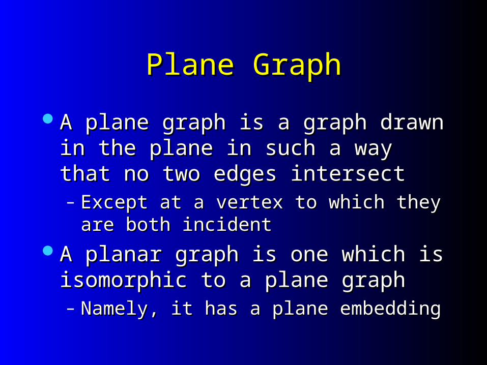
A plane graph is a graph drawn in the A plane graph is a graph drawn in the plane in such a way that no two edges plane in such a way that no two edges intersectintersect– Except at a vertex to which they are both Except at a vertex to which they are both
incidentincidentA planar graph is one which is A planar graph is one which is
isomorphic to a plane graphisomorphic to a plane graph– Namely, it has a plane embeddingNamely, it has a plane embedding

Planar GraphsPlanar Graphs

Planar Graph EmbeddingPlanar Graph EmbeddingClockwise edge orderingClockwise edge ordering
Issues in Planarity TestIssues in Planarity Test
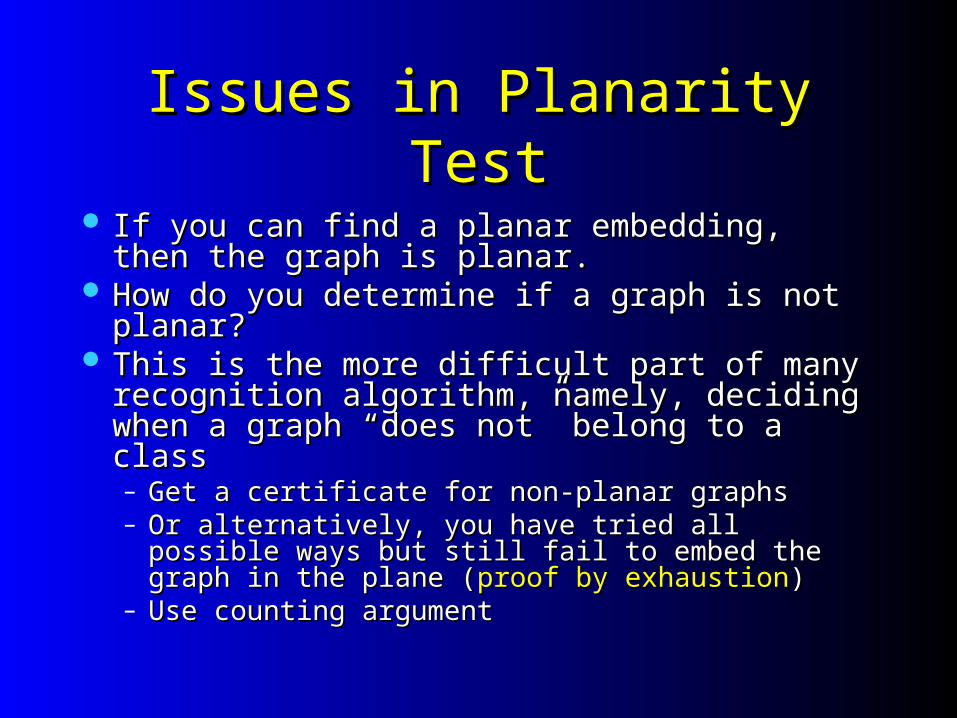
If you can find a planar embedding, then the If you can find a planar embedding, then the graph is planar.graph is planar.
How do you determine if a graph is not planar?How do you determine if a graph is not planar? This is the more difficult part of many This is the more difficult part of many
recognition algorithm, namely, deciding when a recognition algorithm, namely, deciding when a graph “does not” belong to a classgraph “does not” belong to a class– Get a certificate for non-planar graphsGet a certificate for non-planar graphs– Or alternatively, you have tried all possible ways but Or alternatively, you have tried all possible ways but
still fail to embed the graph in the plane (still fail to embed the graph in the plane (proof by proof by exhaustionexhaustion))
– Use counting argumentUse counting argument

Basic Non-Planar GraphsBasic Non-Planar Graphs
K5K3,3

Euler’s Theorem (1752)Euler’s Theorem (1752)
Euler’s theoremEuler’s theoremLet Let GG be a connected plane graph, and let be a connected plane graph, and let ff be the # of faces of be the # of faces of GG..Then Then n + f = mn + f = m + 2 + 2– Prove by induction on the # of edges.Prove by induction on the # of edges.
Corollary. Corollary. mm 33nn – 6 – 6– First show that First show that 33f f 22m m since every face is since every face is
bounded by at lest 3 edgesbounded by at lest 3 edges

KK55 and and KK3,33,3 are non-planar are non-planar
If If KK55 is planar, then by previous is planar, then by previous
Corollary, we have 10 Corollary, we have 10 9. 9. KK3,33,3 is bipartite. Assume it is planar, then is bipartite. Assume it is planar, then
every face is even (has at least 4 every face is even (has at least 4 edges). edges). – Hence 4Hence 4ff 2 2m.m.– Namely, 10 = 2Namely, 10 = 2ff m m = 9.= 9.

Kuratowski’s TheoremKuratowski’s Theorem
Two graphs are Two graphs are homeomorphichomeomorphic if they if they can be obtained from the same graph can be obtained from the same graph by inserting new vertices of degree 2 by inserting new vertices of degree 2 into its edgesinto its edges
A graph is planar if and only if it A graph is planar if and only if it contains no subgraph homeomorphic to contains no subgraph homeomorphic to KK55 or or KK3,33,3
The latter are referred to as The latter are referred to as Kuratowski Kuratowski subgraphssubgraphs

Planarity TestPlanarity Test

How do you draw a planar graph How do you draw a planar graph without regret ?without regret ?
This means that, besides keeping the This means that, besides keeping the current embedding planar, your current embedding planar, your embedding can also keep future embedding can also keep future options open.options open.
You will have to design an embedding You will have to design an embedding “scheme” rather than obtain a “physical” “scheme” rather than obtain a “physical” (( 實體的實體的 ) embedding) embedding

Prior ResultsPrior Results 11st approachst approach
– Hopcroft and Tarjan [1974],first O(Hopcroft and Tarjan [1974],first O(mm) time.) time. – PATH ADDITIONPATH ADDITION
2nd approach2nd approach– Lempel, Even and Cederbaum[1967], O(Lempel, Even and Cederbaum[1967], O(nn22) time) time– VERTEX ADDITIONVERTEX ADDITION– st-numbering, consecutive ones testingst-numbering, consecutive ones testing– Booth and Lueker [1976] used PQ-trees to test theBooth and Lueker [1976] used PQ-trees to test the consecutive ones property in O(consecutive ones property in O(m+nm+n) time) time
3rd approach3rd approach– Shih and Hsu [1999] used PC-trees for recognition and Shih and Hsu [1999] used PC-trees for recognition and
embedding. embedding. – EDGE ADDITIONEDGE ADDITION

A Brief Intro. to the Vertex A Brief Intro. to the Vertex Addition Approach of LECAddition Approach of LEC
Vertex Addition Approach of LECVertex Addition Approach of LEC
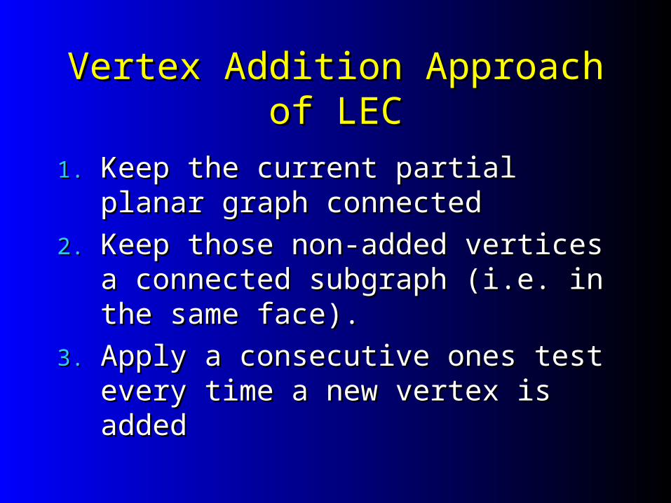
1.1. Keep the current partial planar graph Keep the current partial planar graph connectedconnected
2.2. Keep those non-added vertices a Keep those non-added vertices a connected subgraph (i.e. in the same connected subgraph (i.e. in the same face).face).
3.3. Apply a consecutive ones test every Apply a consecutive ones test every time a new vertex is addedtime a new vertex is added

st-numbering (I)st-numbering (I)
Consider a 2-connected graph Consider a 2-connected graph GG. Pick any two . Pick any two adjacent vertices adjacent vertices ss and and tt..
Order the vertices of G into Order the vertices of G into ss, , vv(1), ..., (1), ..., vv((kk), ), tt such such thatthat
s
sv(i)
v(i)
v(i+1)
v(i+1),…, t must be imbedded in the same face
t
t

St-numbering(II)
s v(i) t
s v(i) tv(i+1)
v(i+1)
Depth-First-SearchDepth-First-Search
s v(i) tv(i+1)

1=s
6=t 2 3 5 6 2 3 5(a) B1 (a’)
(b) B2 (b’)
1
2
6 3 54 53 6 3 54 53
Bush Form (1)Bush Form (1)

(c) B2’
1
2
6 354 53
(c’)
6 54 533
(d) B3
1
2
6 54 5
(d’)
6 54 5644 6
3
Bush Form (2)Bush Form (2)

(e) B3’
2
6 5 4 54 6
3
(e’)
6 5 4 564
(f’)
6 5 4 564
(f) B4
2
6 5 56
3
1
1
65
4
Bush Form (3)Bush Form (3)

(g) B4’
2
6 5 56
3
1
6 5
4
(g’)
6 5 56 6 5
(h’)
6 6 66
(h) B5
2
6 6
3
1
6
54
6
Bush Form (4)Bush Form (4)

(i) G=G6=B6
2
6
3
1
54
(i’)
Bush Form (5)Bush Form (5)
Introducing PQ-TreesIntroducing PQ-Trees
23/30
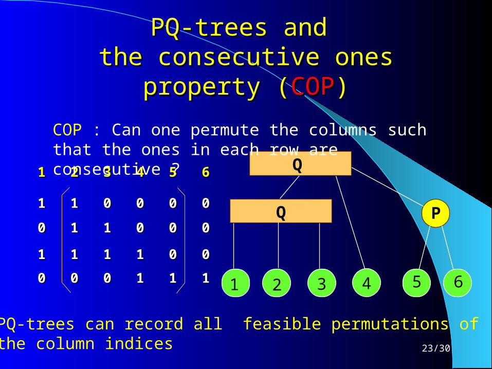
PQ-trees and PQ-trees and the consecutive ones property (the consecutive ones property (COPCOP))
PQ-trees can record all feasible permutations of the column indices
Q P
1 2 3 5 6
Q
4
1 2 3 4 5 61 2 3 4 5 6
1 1 0 0 0 01 1 0 0 0 0
0 1 1 0 0 00 1 1 0 0 0
1 1 1 1 0 01 1 1 1 0 0
0 0 0 1 1 10 0 0 1 1 1
COP : Can one permute the columns such that the ones in each row are consecutive ?
24/30
Linear time algorithm on PQ-treesLinear time algorithm on PQ-trees
[1974] [1974] Booth and Lueker presented a Booth and Lueker presented a linear time algorithm for the COP test linear time algorithm for the COP test based on PQ-treesbased on PQ-trees– Process the matrix one row at a timeProcess the matrix one row at a time
PQ-tree can also be used to yield a PQ-tree can also be used to yield a linear time algorithm for interval graph linear time algorithm for interval graph recognition and planar graph recognition and planar graph recognition.recognition.

25/30
Operations on PQ-trees (I)Operations on PQ-trees (I)
Booth and Lueker’s algorithm is a Booth and Lueker’s algorithm is a bottom-upbottom-up approach consisting of two stages:approach consisting of two stages:– 1. 1. Node labelingNode labeling
The leaves of the incoming row are labeled The leaves of the incoming row are labeled fullfull,, all the all the other leaves are other leaves are emptyempty. the remaining nodes are labeled. the remaining nodes are labeled
emptyempty : all of its children are empty : all of its children are empty full full : all of its children are full: all of its children are full partial partial : neither full nor empty: neither full nor empty
– 2. 2. Tree modificationTree modification

26/30
Operations on PQ-trees (II):Operations on PQ-trees (II):
1. Node labeling 1. Node labelingThe first time a node The first time a node uu becomes partial becomes partial
or full report to its parent.or full report to its parent.The first time a node The first time a node uu gets a partial or gets a partial or
full child label full child label uu partialpartial..The first time all children of a node The first time all children of a node uu
become full label become full label uu fullfull..

27/30
Operations on PQ-trees (III):Operations on PQ-trees (III):
2. Tree modification2. Tree modification Need to modify the current tree so that all the Need to modify the current tree so that all the
incoming columns can be arranged incoming columns can be arranged consecutively. consecutively.
Modify the subtree of every partial nodeModify the subtree of every partial node– At each iteration, modify the subtree of a partial At each iteration, modify the subtree of a partial
node starting from the lowest level of the treenode starting from the lowest level of the tree The subtree modification is based on 9 The subtree modification is based on 9
templates of subtree structurestemplates of subtree structures..

28/30
......
...
...
Template Template PP2 for ROOT (2 for ROOT (T,ST,S) ) when it is a when it is a P-P-nodenode
29/30
......
......
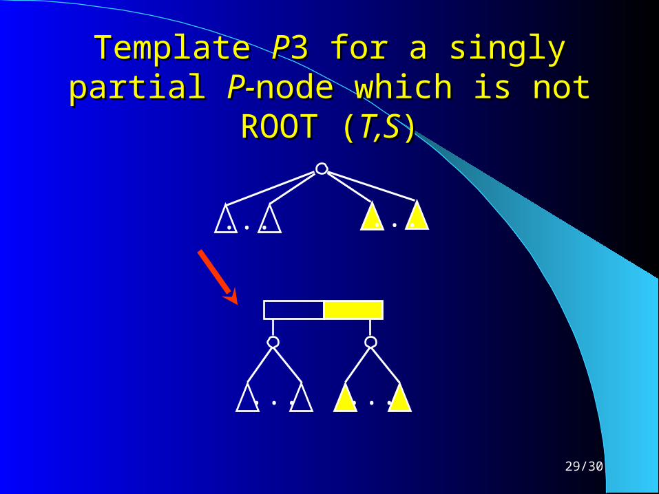
Template Template PP3 for a singly partial 3 for a singly partial P-P-node which is not ROOT (node which is not ROOT (T,ST,S))

30/30
... ...
... ...
Template Template PP4 for ROOT(4 for ROOT(TT,,SS) when it ) when it is a is a PP-node with one partial child-node with one partial child
...... ...
...
31/30
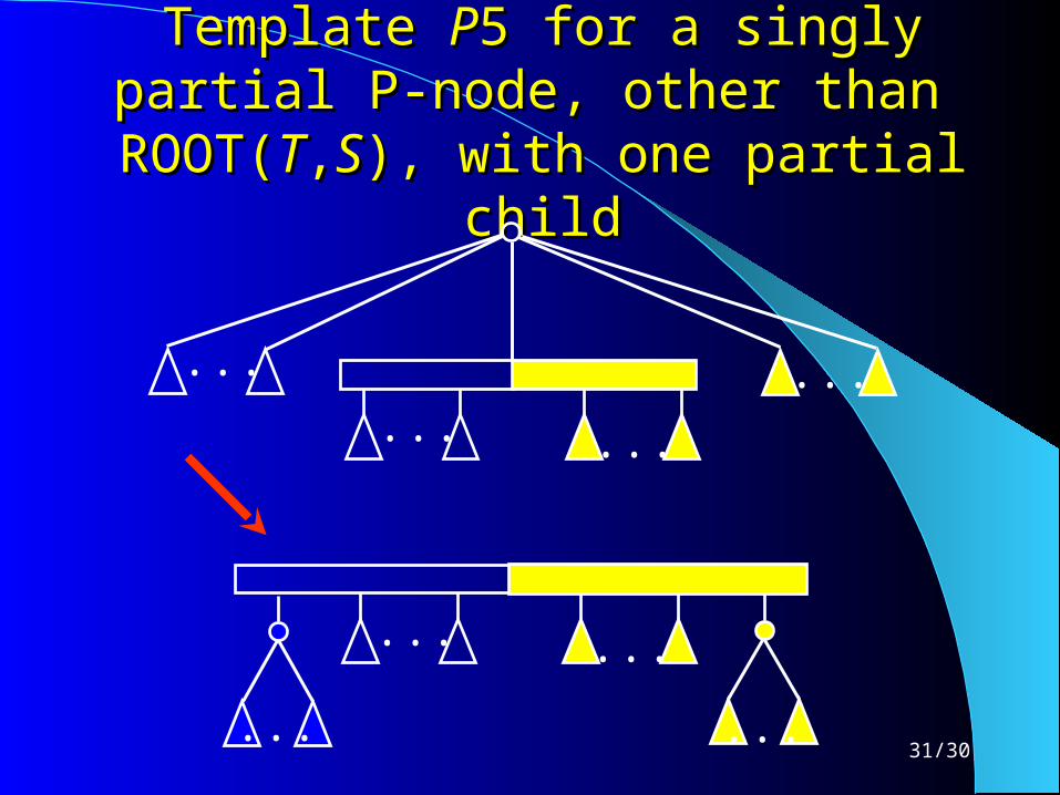
Template Template PP5 for a singly partial P-node, 5 for a singly partial P-node, other than ROOT(other than ROOT(TT,,SS), with one partial ), with one partial
childchild
... ...
... ...
... ...
... ...

32/30
Template PTemplate P66 for ROOT( for ROOT(TT,,SS) when it ) when it is a doubly partial is a doubly partial PP-node-node
......
...
...
... ...
...... ...... ...

33/30
... ......
... ... ......
Template Template Q2Q2 for a singly partial for a singly partial Q-Q-nodenode

34/30
Template Template Q3Q3 for a double partial for a double partial Q-Q-nodenode
... ...... .........
... ... ... ...
...... ...
35/30
Time complexity of the original Time complexity of the original PQ-tree operationsPQ-tree operations
Node labeling takes time proportional to the Node labeling takes time proportional to the number of incoming columns.number of incoming columns.
Subtree modification needs to change many Subtree modification needs to change many parent-children relationshipsparent-children relationships– use amortized analysis to argue that it takes use amortized analysis to argue that it takes
constant time at every iteration.constant time at every iteration.– this analysis is quite involved.this analysis is quite involved.
Does not render a direct algorithm for testing Does not render a direct algorithm for testing the the circular ones propertycircular ones property– Complement a rowComplement a row