Embed Size (px)
Citation preview

Introduction to finite element methods
Hans Petter Langtangen1,2
1Center for Biomedical Computing, Simula Research Laboratory2Department of Informatics, University of Oslo
Dec 16, 2013
PRELIMINARY VERSION
Contents
1 Approximation of vectors 71.1 Approximation of planar vectors . . . . . . . . . . . . . . . . . . 71.2 Approximation of general vectors . . . . . . . . . . . . . . . . . . 11
2 Approximation of functions 132.1 The least squares method . . . . . . . . . . . . . . . . . . . . . . 142.2 The projection (or Galerkin) method . . . . . . . . . . . . . . . . 152.3 Example: linear approximation . . . . . . . . . . . . . . . . . . . 152.4 Implementation of the least squares method . . . . . . . . . . . . 162.5 Perfect approximation . . . . . . . . . . . . . . . . . . . . . . . . 172.6 Ill-conditioning . . . . . . . . . . . . . . . . . . . . . . . . . . . . 182.7 Fourier series . . . . . . . . . . . . . . . . . . . . . . . . . . . . . 202.8 Orthogonal basis functions . . . . . . . . . . . . . . . . . . . . . . 222.9 Numerical computations . . . . . . . . . . . . . . . . . . . . . . . 232.10 The interpolation (or collocation) method . . . . . . . . . . . . . 242.11 Lagrange polynomials . . . . . . . . . . . . . . . . . . . . . . . . 26
3 Finite element basis functions 323.1 Elements and nodes . . . . . . . . . . . . . . . . . . . . . . . . . 333.2 The basis functions . . . . . . . . . . . . . . . . . . . . . . . . . . 353.3 Example on piecewise quadratic finite element functions . . . . . 373.4 Example on piecewise linear finite element functions . . . . . . . 383.5 Example on piecewise cubic finite element basis functions . . . . 403.6 Calculating the linear system . . . . . . . . . . . . . . . . . . . . 413.7 Assembly of elementwise computations . . . . . . . . . . . . . . . 443.8 Mapping to a reference element . . . . . . . . . . . . . . . . . . . 473.9 Example: Integration over a reference element . . . . . . . . . . . 49

4 Implementation 504.1 Integration . . . . . . . . . . . . . . . . . . . . . . . . . . . . . . 514.2 Linear system assembly and solution . . . . . . . . . . . . . . . . 534.3 Example on computing symbolic approximations . . . . . . . . . 534.4 Comparison with finite elements and interpolation/collocation . . 544.5 Example on computing numerical approximations . . . . . . . . . 544.6 The structure of the coefficient matrix . . . . . . . . . . . . . . . 554.7 Applications . . . . . . . . . . . . . . . . . . . . . . . . . . . . . . 574.8 Sparse matrix storage and solution . . . . . . . . . . . . . . . . . 58
5 Comparison of finite element and finite difference approxima-tion 595.1 Finite difference approximation of given functions . . . . . . . . . 605.2 Finite difference interpretation of a finite element approximation 605.3 Making finite elements behave as finite differences . . . . . . . . 62
6 A generalized element concept 636.1 Cells, vertices, and degrees of freedom . . . . . . . . . . . . . . . 646.2 Extended finite element concept . . . . . . . . . . . . . . . . . . . 646.3 Implementation . . . . . . . . . . . . . . . . . . . . . . . . . . . . 656.4 Computing the error of the approximation . . . . . . . . . . . . . 666.5 Example: Cubic Hermite polynomials . . . . . . . . . . . . . . . 68
7 Numerical integration 697.1 Newton-Cotes rules . . . . . . . . . . . . . . . . . . . . . . . . . . 697.2 Gauss-Legendre rules with optimized points . . . . . . . . . . . . 70
8 Approximation of functions in 2D 708.1 2D basis functions as tensor products of 1D functions . . . . . . 718.2 Example: Polynomial basis in 2D . . . . . . . . . . . . . . . . . . 728.3 Implementation . . . . . . . . . . . . . . . . . . . . . . . . . . . . 748.4 Extension to 3D . . . . . . . . . . . . . . . . . . . . . . . . . . . 76
9 Finite elements in 2D and 3D 769.1 Basis functions over triangles in the physical domain . . . . . . . 779.2 Basis functions over triangles in the reference cell . . . . . . . . . 789.3 Affine mapping of the reference cell . . . . . . . . . . . . . . . . . 819.4 Isoparametric mapping of the reference cell . . . . . . . . . . . . 829.5 Computing integrals . . . . . . . . . . . . . . . . . . . . . . . . . 83
10 Exercises 84
11 Basic principles for approximating differential equations 9011.1 Differential equation models . . . . . . . . . . . . . . . . . . . . . 9011.2 Simple model problems . . . . . . . . . . . . . . . . . . . . . . . 9211.3 Forming the residual . . . . . . . . . . . . . . . . . . . . . . . . . 9311.4 The least squares method . . . . . . . . . . . . . . . . . . . . . . 94
2

11.5 The Galerkin method . . . . . . . . . . . . . . . . . . . . . . . . 94
11.6 The Method of Weighted Residuals . . . . . . . . . . . . . . . . . 94
11.7 Test and Trial Functions . . . . . . . . . . . . . . . . . . . . . . . 95
11.8 The collocation method . . . . . . . . . . . . . . . . . . . . . . . 95
11.9 Examples on using the principles . . . . . . . . . . . . . . . . . . 97
11.10Integration by parts . . . . . . . . . . . . . . . . . . . . . . . . . 100
11.11Boundary function . . . . . . . . . . . . . . . . . . . . . . . . . . 101
11.12Abstract notation for variational formulations . . . . . . . . . . . 103
11.13Variational problems and optimization of functionals . . . . . . . 104
12 Examples on variational formulations 105
12.1 Variable coefficient . . . . . . . . . . . . . . . . . . . . . . . . . . 105
12.2 First-order derivative in the equation and boundary condition . . 107
12.3 Nonlinear coefficient . . . . . . . . . . . . . . . . . . . . . . . . . 108
12.4 Computing with Dirichlet and Neumann conditions . . . . . . . . 109
12.5 When the numerical method is exact . . . . . . . . . . . . . . . . 110
13 Computing with finite elements 110
13.1 Finite element mesh and basis functions . . . . . . . . . . . . . . 111
13.2 Computation in the global physical domain . . . . . . . . . . . . 111
13.3 Comparison with a finite difference discretization . . . . . . . . . 114
13.4 Cellwise computations . . . . . . . . . . . . . . . . . . . . . . . . 114
14 Boundary conditions: specified nonzero value 117
14.1 General construction of a boundary function . . . . . . . . . . . . 117
14.2 Example on computing with finite element-based a boundaryfunction . . . . . . . . . . . . . . . . . . . . . . . . . . . . . . . . 119
14.3 Modification of the linear system . . . . . . . . . . . . . . . . . . 120
14.4 Symmetric modification of the linear system . . . . . . . . . . . . 123
14.5 Modification of the element matrix and vector . . . . . . . . . . . 124
15 Boundary conditions: specified derivative 125
15.1 The variational formulation . . . . . . . . . . . . . . . . . . . . . 125
15.2 Boundary term vanishes because of the test functions . . . . . . 125
15.3 Boundary term vanishes because of linear system modifications . 126
15.4 Direct computation of the global linear system . . . . . . . . . . 126
15.5 Cellwise computations . . . . . . . . . . . . . . . . . . . . . . . . 128
16 Implementation 129
16.1 Global basis functions . . . . . . . . . . . . . . . . . . . . . . . . 129
16.2 Example: constant right-hand side . . . . . . . . . . . . . . . . . 131
16.3 Finite elements . . . . . . . . . . . . . . . . . . . . . . . . . . . . 132
3

17 Variational formulations in 2D and 3D 13417.1 Transformation to a reference cell in 2D and 3D . . . . . . . . . . 13617.2 Numerical integration . . . . . . . . . . . . . . . . . . . . . . . . 13717.3 Convenient formulas for P1 elements in 2D . . . . . . . . . . . . 138
18 Summary 139
19 Time-dependent problems 14119.1 Discretization in time by a Forward Euler scheme . . . . . . . . . 14119.2 Variational forms . . . . . . . . . . . . . . . . . . . . . . . . . . . 14219.3 Simplified notation for the solution at recent time levels . . . . . 14319.4 Deriving the linear systems . . . . . . . . . . . . . . . . . . . . . 14319.5 Computational algorithm . . . . . . . . . . . . . . . . . . . . . . 14519.6 Comparing P1 elements with the finite difference method . . . . 14519.7 Discretization in time by a Backward Euler scheme . . . . . . . . 14619.8 Dirichlet boundary conditions . . . . . . . . . . . . . . . . . . . . 14719.9 Example: Oscillating Dirichlet boundary condition . . . . . . . . 14919.10Analysis of the discrete equations . . . . . . . . . . . . . . . . . . 151
20 Systems of differential equations 15620.1 Variational forms . . . . . . . . . . . . . . . . . . . . . . . . . . . 15620.2 A worked example . . . . . . . . . . . . . . . . . . . . . . . . . . 15720.3 Identical function spaces for the unknowns . . . . . . . . . . . . . 15820.4 Different function spaces for the unknowns . . . . . . . . . . . . . 16220.5 Computations in 1D . . . . . . . . . . . . . . . . . . . . . . . . . 163
21 Exercises 164
4

List of Exercises and Problems
Exercise 1 Linear algebra refresher I p. 84Exercise 2 Linear algebra refresher II p. 84Exercise 3 Approximate a three-dimensional vector in ... p. 84Exercise 4 Approximate the exponential function by power ... p. 85Exercise 5 Approximate the sine function by power functions ... p. 85Exercise 6 Approximate a steep function by sines p. 85Exercise 7 Animate the approximation of a steep function ... p. 85Exercise 8 Fourier series as a least squares approximation ... p. 86Exercise 9 Approximate a steep function by Lagrange polynomials ... p. 87Exercise 10 Define nodes and elements p. 86Exercise 11 Define vertices, cells, and dof maps p. 87Exercise 12 Construct matrix sparsity patterns p. 87Exercise 13 Perform symbolic finite element computations p. 87Exercise 14 Approximate a steep function by P1 and P2 ... p. 87Exercise 15 Approximate a steep function by P3 and P4 ... p. 87Exercise 16 Investigate the approximation error in finite ... p. 87Exercise 17 Approximate a step function by finite elements ... p. 88Exercise 18 2D approximation with orthogonal functions p. 88Exercise 19 Use the Trapezoidal rule and P1 elements p. 89Problem 20 Compare P1 elements and interpolation p. 89Exercise 21 Implement 3D computations with global basis ... p. 90Exercise 22 Use Simpson’s rule and P2 elements p. 90Exercise 23 Refactor functions into a more general class p. 164Exercise 24 Compute the deflection of a cable with sine ... p. 164Exercise 25 Check integration by parts p. 165Exercise 26 Compute the deflection of a cable with 2 P1 ... p. 165Exercise 27 Compute the deflection of a cable with 1 P2 ... p. 165Exercise 28 Compute the deflection of a cable with a step ... p. 165Exercise 29 Show equivalence between linear systems p. 166Exercise 30 Compute with a non-uniform mesh p. 166Problem 31 Solve a 1D finite element problem by hand p. 166Exercise 32 Compare finite elements and differences for ... p. 167Exercise 33 Compute with variable coefficients and P1 ... p. 168Exercise 34 Solve a 2D Poisson equation using polynomials ... p. 168Exercise 35 Analyze a Crank-Nicolson scheme for the diffusion ... p. 169
5

The finite element method is a powerful tool for solving differential equations.The method can easily deal with complex geometries and higher-order approxima-tions of the solution. Figure 1 shows a two-dimensional domain with a non-trivialgeometry. The idea is to divide the domain into triangles (elements) and seeka polynomial approximations to the unknown functions on each triangle. Themethod glues these piecewise approximations together to find a global solution.Linear and quadratic polynomials over the triangles are particularly popular.
Figure 1: Domain for flow around a dolphin.
Many successful numerical methods for differential equations, including thefinite element method, aim at approximating the unknown function by a sum
u(x) =
N∑i=0
ciψi(x), (1)
where ψi(x) are prescribed functions and c0, . . . , cN are unknown coefficients tobe determined. Solution methods for differential equations utilizing (1) musthave a principle for constructing N + 1 equations to determine c0, . . . , cN . Thenthere is a machinery regarding the actual constructions of the equations forc0, . . . , cN , in a particular problem. Finally, there is a solve phase for computingthe solution c0, . . . , cN of the N + 1 equations.
6

Especially in the finite element method, the machinery for constructing thediscrete equations to be implemented on a computer is quite comprehensive, withmany mathematical and implementational details entering the scene at the sametime. From an ease-of-learning perspective it can therefore be wise to introducethe computational machinery for a trivial equation: u = f . Solving this equationwith f given and u on the form (1) means that we seek an approximationu to f . This approximation problem has the advantage of introducing mostof the finite element toolbox, but with postponing demanding topics relatedto differential equations (e.g., integration by parts, boundary conditions, andcoordinate mappings). This is the reason why we shall first become familiarwith finite element approximation before addressing finite element methods fordifferential equations.
First, we refresh some linear algebra concepts about approximating vectorsin vector spaces. Second, we extend these concepts to approximating functionsin function spaces, using the same principles and the same notation. We presentexamples on approximating functions by global basis functions with supportthroughout the entire domain. Third, we introduce the finite element type oflocal basis functions and explain the computational algorithms for working withsuch functions. Three types of approximation principles are covered: 1) the leastsquares method, 2) the L2 projection or Galerkin method, and 3) interpolationor collocation.
1 Approximation of vectors
We shall start with introducing two fundamental methods for determining thecoefficients ci in (1) and illustrate the methods on approximation of vectors,because vectors in vector spaces give a more intuitive understanding than startingdirectly with approximation of functions in function spaces. The extensionfrom vectors to functions will be trivial as soon as the fundamental ideas areunderstood.
The first method of approximation is called the least squares method andconsists in finding ci such that the difference u− f , measured in some norm, isminimized. That is, we aim at finding the best approximation u to f (in somenorm). The second method is not as intuitive: we find u such that the erroru− f is orthogonal to the space where we seek u. This is known as projection,or we may also call it a Galerkin method. When approximating vectors andfunctions, the two methods are equivalent, but this is no longer the case whenapplying the principles to differential equations.
1.1 Approximation of planar vectors
Suppose we have given a vector f = (3, 5) in the xy plane and that we want toapproximate this vector by a vector aligned in the direction of the vector (a, b).Figure 2 depicts the situation.
We introduce the vector space V spanned by the vector ψ0 = (a, b):
7

0
1
2
3
4
5
6
0 1 2 3 4 5 6
(a,b)
(3,5)
c0(a,b)
Figure 2: Approximation of a two-dimensional vector by a one-dimensionalvector.
V = span ψ0 . (2)
We say that ψ0 is a basis vector in the space V . Our aim is to find thevector u = c0ψ0 ∈ V which best approximates the given vector f = (3, 5). Areasonable criterion for a best approximation could be to minimize the length ofthe difference between the approximate u and the given f . The difference, orerror e = f − u, has its length given by the norm
||e|| = (e, e)12 ,
where (e, e) is the inner product of e and itself. The inner product, also calledscalar product or dot product, of two vectors u = (u0, u1) and v = (v0, v1) isdefined as
(u,v) = u0v0 + u1v1 . (3)
8

Remark 1. We should point out that we use the notation (·, ·) for two differentthings: (a, b) for scalar quantities a and b means the vector starting in the originand ending in the point (a, b), while (u,v) with vectors u and v means the innerproduct of these vectors. Since vectors are here written in boldface font thereshould be no confusion. We may add that the norm associated with this innerproduct is the usual Eucledian length of a vector.
Remark 2. It might be wise to refresh some basic linear algebra by consultinga textbook. Exercises 1 and 2 suggest specific tasks to regain familiarity withfundamental operations on inner product vector spaces.
The least squares method. We now want to find c0 such that it minimizes||e||. The algebra is simplified if we minimize the square of the norm, ||e||2 =(e, e), instead of the norm itself. Define the function
E(c0) = (e, e) = (f − c0ψ0,f − c0ψ0) . (4)
We can rewrite the expressions of the right-hand side in a more convenient formfor further work:
E(c0) = (f ,f)− 2c0(f ,ψ0) + c20(ψ0,ψ0) . (5)
The rewrite results from using the following fundamental rules for inner productspaces:
(αu,v) = α(u,v), α ∈ R, (6)
(u+ v,w) = (u,w) + (v,w), (7)
(u,v) = (v,u) . (8)
Minimizing E(c0) implies finding c0 such that
∂E
∂c0= 0 .
Differentiating (5) with respect to c0 gives
∂E
∂c0= −2(f ,ψ0) + 2c0(ψ0,ψ0) . (9)
Setting the above expression equal to zero and solving for c0 gives
c0 =(f ,ψ0)
(ψ0,ψ0), (10)
which in the present case with ψ0 = (a, b) results in
9
c0 =3a+ 5b
a2 + b2. (11)
For later, it is worth mentioning that setting the key equation (9) to zerocan be rewritten as
(f − c0ψ0,ψ0) = 0,
or
(e,ψ0) = 0 . (12)
The projection method. We shall now show that minimizing ||e||2 impliesthat e is orthogonal to any vector v in the space V . This result is visually quiteclear from Figure 2 (think of other vectors along the line (a, b): all of them willlead to a larger distance between the approximation and f). To see this resultmathematically, we express any v ∈ V as v = sψ0 for any scalar parameter s,recall that two vectors are orthogonal when their inner product vanishes, andcalculate the inner product
(e, sψ0) = (f − c0ψ0, sψ0)
= (f , sψ0)− (c0ψ0, sψ0)
= s(f ,ψ0)− sc0(ψ0,ψ0)
= s(f ,ψ0)− s (f ,ψ0)
(ψ0,ψ0)(ψ0,ψ0)
= s ((f ,ψ0)− (f ,ψ0))
= 0 .
Therefore, instead of minimizing the square of the norm, we could demand thate is orthogonal to any vector in V . This method is known as projection, becauseit is the same as projecting the vector onto the subspace. (The approach canalso be referred to as a Galerkin method as explained at the end of Section ??.)
Mathematically the projection method is stated by the equation
(e,v) = 0, ∀v ∈ V . (13)
An arbitrary v ∈ V can be expressed as sψ0, s ∈ R, and therefore (13) implies
(e, sψ0) = s(e,ψ0) = 0,
which means that the error must be orthogonal to the basis vector in the spaceV :
(e,ψ0) = 0 or (f − c0ψ0,ψ0) = 0 .
The latter equation gives (10) and it also arose from least squares computationsin (12).
10
1.2 Approximation of general vectors
Let us generalize the vector approximation from the previous section to vectorsin spaces with arbitrary dimension. Given some vector f , we want to find thebest approximation to this vector in the space
V = span ψ0, . . . ,ψN .We assume that the basis vectors ψ0, . . . ,ψN are linearly independent so thatnone of them are redundant and the space has dimension N + 1. Any vectoru ∈ V can be written as a linear combination of the basis vectors,
u =
N∑j=0
cjψj ,
where cj ∈ R are scalar coefficients to be determined.
The least squares method. Now we want to find c0, . . . , cN , such that u isthe best approximation to f in the sense that the distance (error) e = f − uis minimized. Again, we define the squared distance as a function of the freeparameters c0, . . . , cN ,
E(c0, . . . , cN ) = (e, e) = (f −∑j
cjψj ,f −∑j
cjψj)
= (f ,f)− 2
N∑j=0
cj(f ,ψj) +
N∑p=0
N∑q=0
cpcq(ψp,ψq) . (14)
Minimizing this E with respect to the independent variables c0, . . . , cN is obtainedby requiring
∂E
∂ci= 0, i = 0, . . . , N .
The second term in (14) is differentiated as follows:
∂
∂ci
N∑j=0
cj(f ,ψj) = (f ,ψi), (15)
since the expression to be differentiated is a sum and only one term, ci(f ,ψi),contains ci and this term is linear in ci. To understand this differentiation indetail, write out the sum specifically for, e.g, N = 3 and i = 1.
The last term in (14) is more tedious to differentiate. We start with
∂
∂cicpcq =
0, if p 6= i and q 6= i,cq, if p = i and q 6= i,cp, if p 6= i and q = i,2ci, if p = q = i,
(16)
11

Then
∂
∂ci
N∑p=0
N∑q=0
cpcq(ψp,ψq) =
N∑p=0,p6=i
cp(ψp,ψi) +
N∑q=0,q 6=i
cq(ψq,ψi) + 2ci(ψi,ψi) .
The last term can be included in the other two sums, resulting in
∂
∂ci
N∑p=0
N∑q=0
cpcq(ψp,ψq) = 2
N∑j=0
ci(ψj ,ψi) . (17)
It then follows that setting
∂E
∂ci= 0, i = 0, . . . , N,
leads to a linear system for c0, . . . , cN :
N∑j=0
Ai,jcj = bi, i = 0, . . . , N, (18)
where
Ai,j = (ψi,ψj), (19)
bi = (ψi,f) . (20)
We have changed the order of the two vectors in the inner product according to(1.1):
Ai,j = (ψj ,ψi) = (ψi,ψj),
simply because the sequence i-j looks more aesthetic.
The Galerkin or projection method. In analogy with the ”one-dimensional”example in Section 1.1, it holds also here in the general case that minimizing thedistance (error) e is equivalent to demanding that e is orthogonal to all v ∈ V :
(e,v) = 0, ∀v ∈ V . (21)
Since any v ∈ V can be written as v =∑Ni=0 ciψi, the statement (21) is
equivalent to saying that
(e,
N∑i=0
ciψi) = 0,
for any choice of coefficients c0, . . . , cN . The latter equation can be rewritten as
12

N∑i=0
ci(e,ψi) = 0 .
If this is to hold for arbitrary values of c0, . . . , cN we must require that eachterm in the sum vanishes,
(e,ψi) = 0, i = 0, . . . , N . (22)
These N + 1 equations result in the same linear system as (18):
(f −N∑j=0
cjψj ,ψi) = (f ,ψi)−∑j∈Is
(ψi,ψj)cj = 0,
and hence
N∑j=0
(ψi,ψj)cj = (f ,ψi), i = 0, . . . , N .
So, instead of differentiating the E(c0, . . . , cN ) function, we could simply use(21) as the principle for determining c0, . . . , cN , resulting in the N + 1 equations(22).
The names least squares method or least squares approximation are naturalsince the calculations consists of minimizing ||e||2, and ||e||2 is a sum of squaresof differences between the components in f and u. We find u such that thissum of squares is minimized.
The principle (21), or the equivalent form (22), is known as projection.Almost the same mathematical idea was used by the Russian mathematicianBoris Galerkin to solve differential equations, resulting in what is widely knownas Galerkin’s method.
2 Approximation of functions
Let V be a function space spanned by a set of basis functions ψ0, . . . , ψN ,
V = span ψ0, . . . , ψN,
such that any function u ∈ V can be written as a linear combination of the basisfunctions:
u =∑j∈Is
cjψj . (23)
The index set Is is defined as Is = 0, . . . , N and is used both for compactnotation and for flexibility in the numbering of elements in sequences.
For now, in this introduction, we shall look at functions of a single variablex: u = u(x), ψi = ψi(x), i ∈ Is. Later, we will almost trivially extend the
13

mathematical details to functions of two- or three-dimensional physical spaces.The approximation (23) is typically used to discretize a problem in space. Othermethods, most notably finite differences, are common for time discretization,although the form (23) can be used in time as well.
2.1 The least squares method
Given a function f(x), how can we determine its best approximation u(x) ∈ V ?A natural starting point is to apply the same reasoning as we did for vectorsin Section 1.2. That is, we minimize the distance between u and f . However,this requires a norm for measuring distances, and a norm is most convenientlydefined through an inner product. Viewing a function as a vector of infinitelymany point values, one for each value of x, the inner product could intuitivelybe defined as the usual summation of pairwise components, with summationreplaced by integration:
(f, g) =
∫f(x)g(x) dx .
To fix the integration domain, we let f(x) and ψi(x) be defined for a domainΩ ⊂ R. The inner product of two functions f(x) and g(x) is then
(f, g) =
∫Ω
f(x)g(x) dx . (24)
The distance between f and any function u ∈ V is simply f − u, and thesquared norm of this distance is
E = (f(x)−∑j∈Is
cjψj(x), f(x)−∑j∈Is
cjψj(x)) . (25)
Note the analogy with (14): the given function f plays the role of the givenvector f , and the basis function ψi plays the role of the basis vector ψi. We canrewrite (25), through similar steps as used for the result (14), leading to
E(ci, . . . , cN ) = (f, f)− 2∑j∈Is
cj(f, ψi) +∑p∈Is
∑q∈Is
cpcq(ψp, ψq) . (26)
Minimizing this function of N+1 scalar variables cii∈Is , requires differentiationwith respect to ci, for all i ∈ Is. The resulting equations are very similar tothose we had in the vector case, and we hence end up with a linear system ofthe form (18), with basically the same expressions:
Ai,j = (ψi, ψj), (27)
bi = (f, ψi) . (28)
14

2.2 The projection (or Galerkin) method
As in Section 1.2, the minimization of (e, e) is equivalent to
(e, v) = 0, ∀v ∈ V . (29)
This is known as a projection of a function f onto the subspace V . We may alsocall it a Galerkin method for approximating functions. Using the same reasoningas in (21)-(22), it follows that (29) is equivalent to
(e, ψi) = 0, i ∈ Is . (30)
Inserting e = f − u in this equation and ordering terms, as in the multi-dimensional vector case, we end up with a linear system with a coefficient matrix(27) and right-hand side vector (28).
Whether we work with vectors in the plane, general vectors, or functionsin function spaces, the least squares principle and the projection or Galerkinmethod are equivalent.
2.3 Example: linear approximation
Let us apply the theory in the previous section to a simple problem: given aparabola f(x) = 10(x− 1)2 − 1 for x ∈ Ω = [1, 2], find the best approximationu(x) in the space of all linear functions:
V = span 1, x .
With our notation, ψ0(x) = 1, ψ1(x) = x, and N = 1. We seek
u = c0ψ0(x) + c1ψ1(x) = c0 + c1x,
where c0 and c1 are found by solving a 2× 2 the linear system. The coefficientmatrix has elements
A0,0 = (ψ0, ψ0) =
∫ 2
1
1 · 1 dx = 1, (31)
A0,1 = (ψ0, ψ1) =
∫ 2
1
1 · x dx = 3/2, (32)
A1,0 = A0,1 = 3/2, (33)
A1,1 = (ψ1, ψ1) =
∫ 2
1
x · x dx = 7/3 . (34)
The corresponding right-hand side is
15

b1 = (f, ψ0) =
∫ 2
1
(10(x− 1)2 − 1) · 1 dx = 7/3, (35)
b2 = (f, ψ1) =
∫ 2
1
(10(x− 1)2 − 1) · x dx = 13/3 . (36)
Solving the linear system results in
c0 = −38/3, c1 = 10, (37)
and consequently
u(x) = 10x− 38
3. (38)
Figure 3 displays the parabola and its best approximation in the space of alllinear functions.
1.0 1.2 1.4 1.6 1.8 2.0 2.2x
4
2
0
2
4
6
8
10
approximationexact
Figure 3: Best approximation of a parabola by a straight line.
2.4 Implementation of the least squares method
The linear system can be computed either symbolically or numerically (a numer-ical integration rule is needed in the latter case). Here is a function for symboliccomputation of the linear system, where f(x) is given as a sympy expression f
16

involving the symbol x, psi is a list of expressions for ψii∈Is , and Omega is a2-tuple/list holding the limits of the domain Ω:
import sympy as sp
def least_squares(f, psi, Omega):N = len(psi) - 1A = sp.zeros((N+1, N+1))b = sp.zeros((N+1, 1))x = sp.Symbol(’x’)for i in range(N+1):
for j in range(i, N+1):A[i,j] = sp.integrate(psi[i]*psi[j],
(x, Omega[0], Omega[1]))A[j,i] = A[i,j]
b[i,0] = sp.integrate(psi[i]*f, (x, Omega[0], Omega[1]))c = A.LUsolve(b)u = 0for i in range(len(psi)):
u += c[i,0]*psi[i]return u, c
Observe that we exploit the symmetry of the coefficient matrix: only theupper triangular part is computed. Symbolic integration in sympy is oftentime consuming, and (roughly) halving the work has noticeable effect on thewaiting time for the function to finish execution.
Comparing the given f(x) and the approximate u(x) visually is done bythe following function, which with the aid of sympy’s lambdify tool converts asympy expression to a Python function for numerical computations:
def comparison_plot(f, u, Omega, filename=’tmp.pdf’):x = sp.Symbol(’x’)f = sp.lambdify([x], f, modules="numpy")u = sp.lambdify([x], u, modules="numpy")resolution = 401 # no of points in plotxcoor = linspace(Omega[0], Omega[1], resolution)exact = f(xcoor)approx = u(xcoor)plot(xcoor, approx)hold(’on’)plot(xcoor, exact)legend([’approximation’, ’exact’])savefig(filename)
The modules=’numpy’ argument to lambdify is important if there are mathe-matical functions, such as sin or exp in the symbolic expressions in f or u, andthese mathematical functions are to be used with vector arguments, like xcoor
above.Both the least_squares and comparison_plot are found and coded in the
file approx1D.py. The forthcoming examples on their use appear in ex_approx1D.py.
2.5 Perfect approximation
Let us use the code above to recompute the problem from Section 2.3 where wewant to approximate a parabola. What happens if we add an element x2 to the
17

basis and test what the best approximation is if V is the space of all parabolicfunctions? The answer is quickly found by running
>>> from approx1D import *>>> x = sp.Symbol(’x’)>>> f = 10*(x-1)**2-1>>> u, c = least_squares(f=f, psi=[1, x, x**2], Omega=[1, 2])>>> print u10*x**2 - 20*x + 9>>> print sp.expand(f)10*x**2 - 20*x + 9
Now, what if we use ψi(x) = xi for i = 0, 1, . . . , N = 40? The output fromleast_squares gives ci = 0 for i > 2, which means that the method finds theperfect approximation.
In fact, we have a general result that if f ∈ V , the least squares andprojection/Galerkin methods compute the exact solution u = f . The proof isstraightforward: if f ∈ V , f can be expanded in terms of the basis functions,f =
∑j∈Is djψj , for some coefficients dii∈Is , and the right-hand side then has
entries
bi = (f, ψi) =∑j∈Is
dj(ψj , ψi) =∑j∈Is
djAi,j .
The linear system∑j Ai,jcj = bi, i ∈ Is, is then
∑j∈Is
cjAi,j =∑j∈Is
djAi,j , i ∈ Is,
which implies that ci = di for i ∈ Is.
2.6 Ill-conditioning
The computational example in Section 2.5 applies the least_squares functionwhich invokes symbolic methods to calculate and solve the linear system. Thecorrect solution c0 = 9, c1 = −20, c2 = 10, ci = 0 for i ≥ 3 is perfectly recovered.
Suppose we convert the matrix and right-hand side to floating-point arraysand then solve the system using finite-precision arithmetics, which is what onewill (almost) always do in real life. This time we get astonishing results! Upto about N = 7 we get a solution that is reasonably close to the exact one.Increasing N shows that seriously wrong coefficients are computed. Below isa table showing the solution of the linear system arising from approximatinga parabola by functions on the form u(x) = c0 + c1x + c2x
2 + · · · + c10x10.
Analytically, we know that cj = 0 for j > 2, but numerically we may get cj 6= 0for j > 2.
18

exact sympy numpy32 numpy64
9 9.62 5.57 8.98-20 -23.39 -7.65 -19.9310 17.74 -4.50 9.960 -9.19 4.13 -0.260 5.25 2.99 0.720 0.18 -1.21 -0.930 -2.48 -0.41 0.730 1.81 -0.013 -0.360 -0.66 0.08 0.110 0.12 0.04 -0.020 -0.001 -0.02 0.002
The exact value of cj , j = 0, 1, . . . , 10, appears in the first column while theother columns correspond to results obtained by three different methods:
• Column 2: The matrix and vector are converted to the data structuresympy.mpmath.fp.matrix and the sympy.mpmath.fp.lu_solve functionis used to solve the system.
• Column 3: The matrix and vector are converted to numpy arrays with datatype numpy.float32 (single precision floating-point number) and solvedby the numpy.linalg.solve function.
• Column 4: As column 3, but the data type is numpy.float64 (doubleprecision floating-point number).
We see from the numbers in the table that double precision performs much betterthan single precision. Nevertheless, when plotting all these solutions the curvescannot be visually distinguished (!). This means that the approximations lookperfect, despite the partially very wrong values of the coefficients.
Increasing N to 12 makes the numerical solver in numpy abort with themessage: ”matrix is numerically singular”. A matrix has to be non-singular tobe invertible, which is a requirement when solving a linear system. Already whenthe matrix is close to singular, it is ill-conditioned, which here implies that thenumerical solution algorithms are sensitive to round-off errors and may produce(very) inaccurate results.
The reason why the coefficient matrix is nearly singular and ill-conditionedis that our basis functions ψi(x) = xi are nearly linearly dependent for large i.That is, xi and xi+1 are very close for i not very small. This phenomenon isillustrated in Figure 4. There are 15 lines in this figure, but only half of themare visually distinguishable. Almost linearly dependent basis functions give riseto an ill-conditioned and almost singular matrix. This fact can be illustrated bycomputing the determinant, which is indeed very close to zero (recall that a zerodeterminant implies a singular and non-invertible matrix): 10−65 for N = 10 and10−92 for N = 12. Already for N = 28 the numerical determinant computationreturns a plain zero.
19

1.0 1.2 1.4 1.6 1.8 2.0 2.20
2000
4000
6000
8000
10000
12000
14000
16000
18000
Figure 4: The 15 first basis functions xi, i = 0, . . . , 14.
On the other hand, the double precision numpy solver do run for N = 100,resulting in answers that are not significantly worse than those in the tableabove, and large powers are associated with small coefficients (e.g., cj < 10−2
for 10 ≤ j ≤ 20 and c < 10−5 for j > 20). Even for N = 100 the approximationstill lies on top of the exact curve in a plot (!).
The conclusion is that visual inspection of the quality of the approximationmay not uncover fundamental numerical problems with the computations. How-ever, numerical analysts have studied approximations and ill-conditioning fordecades, and it is well known that the basis 1, x, x2, x3, . . . , is a bad basis.The best basis from a matrix conditioning point of view is to have orthogonalfunctions such that (ψi, ψj) = 0 for i 6= j. There are many known sets of orthog-onal polynomials and other functions. The functions used in the finite elementmethods are almost orthogonal, and this property helps to avoid problems withsolving matrix systems. Almost orthogonal is helpful, but not enough whenit comes to partial differential equations, and ill-conditioning of the coefficientmatrix is a theme when solving large-scale matrix systems arising from finiteelement discretizations.
2.7 Fourier series
A set of sine functions is widely used for approximating functions (the sines arealso orthogonal as explained more in Section 2.6). Let us take
20

V = span sinπx, sin 2πx, . . . , sin(N + 1)πx .
That is,
ψi(x) = sin((i+ 1)πx), i ∈ Is .
An approximation to the f(x) function from Section 2.3 can then be computedby the least_squares function from Section 2.4:
N = 3from sympy import sin, pix = sp.Symbol(’x’)psi = [sin(pi*(i+1)*x) for i in range(N+1)]f = 10*(x-1)**2 - 1Omega = [0, 1]u, c = least_squares(f, psi, Omega)comparison_plot(f, u, Omega)
Figure 5 (left) shows the oscillatory approximation of∑Nj=0 cj sin((j + 1)πx)
when N = 3. Changing N to 11 improves the approximation considerably, seeFigure 5 (right).
0.0 0.2 0.4 0.6 0.8 1.0x
2
0
2
4
6
8
10
approximationexact
0.0 0.2 0.4 0.6 0.8 1.0x
2
0
2
4
6
8
10
approximationexact
Figure 5: Best approximation of a parabola by a sum of 3 (left) and 11 (right)sine functions.
There is an error f(0)− u(0) = 9 at x = 0 in Figure 5 regardless of how largeN is, because all ψi(0) = 0 and hence u(0) = 0. We may help the approximationto be correct at x = 0 by seeking
u(x) = f(0) +∑j∈Is
cjψj(x) . (39)
However, this adjustment introduces a new problem at x = 1 since we now getan error f(1)− u(1) = f(1)− 0 = −1 at this point. A more clever adjustment isto replace the f(0) term by a term that is f(0) at x = 0 and f(1) at x = 1. Asimple linear combination f(0)(1− x) + xf(1) does the job:
u(x) = f(0)(1− x) + xf(1) +∑j∈Is
cjψj(x) . (40)
21

This adjustment of u alters the linear system slightly as we get an extra term−(f(0)(1− x) + xf(1), ψi) on the right-hand side. Figure 6 shows the result ofthis technique for ensuring right boundary values: even 3 sines can now adjustthe f(0)(1− x) + xf(1) term such that u approximates the parabola really well,at least visually.
0.0 0.2 0.4 0.6 0.8 1.0x
2
0
2
4
6
8
10
approximationexact
0.0 0.2 0.4 0.6 0.8 1.0x
2
0
2
4
6
8
10
approximationexact
Figure 6: Best approximation of a parabola by a sum of 3 (left) and 11 (right)sine functions with a boundary term.
2.8 Orthogonal basis functions
The choice of sine functions ψi(x) = sin((i+ 1)πx) has a great computationaladvantage: on Ω = [0, 1] these basis functions are orthogonal, implying thatAi,j = 0 if i 6= j. This result is realized by trying
integrate(sin(j*pi*x)*sin(k*pi*x), x, 0, 1)
in WolframAlpha (avoid i in the integrand as this symbol means the imaginary
unit√−1). Also by asking WolframAlpha about
∫ 1
0sin2(jπx) dx, we find it to
equal 1/2. With a diagonal matrix we can easily solve for the coefficients byhand:
ci = 2
∫ 1
0
f(x) sin((i+ 1)πx) dx, i ∈ Is, (41)
which is nothing but the classical formula for the coefficients of the Fourier sineseries of f(x) on [0, 1]. In fact, when V contains the basic functions used in aFourier series expansion, the approximation method derived in Section 2 resultsin the classical Fourier series for f(x) (see Exercise 8 for details).
With orthogonal basis functions we can make the least_squares function(much) more efficient since we know that the matrix is diagonal and only thediagonal elements need to be computed:
def least_squares_orth(f, psi, Omega):N = len(psi) - 1A = [0]*(N+1)
22

b = [0]*(N+1)x = sp.Symbol(’x’)for i in range(N+1):
A[i] = sp.integrate(psi[i]**2, (x, Omega[0], Omega[1]))b[i] = sp.integrate(psi[i]*f, (x, Omega[0], Omega[1]))
c = [b[i]/A[i] for i in range(len(b))]u = 0for i in range(len(psi)):
u += c[i]*psi[i]return u, c
This function is found in the file approx1D.py.
2.9 Numerical computations
Sometimes the basis functions ψi and/or the function f have a nature thatmakes symbolic integration CPU-time consuming or impossible. Even though weimplemented a fallback on numerical integration of
∫fϕidx considerable time
might be required by sympy in the attempt to integrate symbolically. Therefore,it will be handy to have function for fast numerical integration and numericalsolution of the linear system. Below is such a method. It requires Pythonfunctions f(x) and psi(x,i) for f(x) and ψi(x) as input. The output is a meshfunction with values u on the mesh with points in the array x. Three numericalintegration methods are offered: scipy.integrate.quad (precision set to 10−8),sympy.mpmath.quad (high precision), and a Trapezoidal rule based on the pointsin x.
def least_squares_numerical(f, psi, N, x,integration_method=’scipy’,orthogonal_basis=False):
import scipy.integrateA = np.zeros((N+1, N+1))b = np.zeros(N+1)Omega = [x[0], x[-1]]dx = x[1] - x[0]
for i in range(N+1):j_limit = i+1 if orthogonal_basis else N+1for j in range(i, j_limit):
print ’(%d,%d)’ % (i, j)if integration_method == ’scipy’:
A_ij = scipy.integrate.quad(lambda x: psi(x,i)*psi(x,j),Omega[0], Omega[1], epsabs=1E-9, epsrel=1E-9)[0]
elif integration_method == ’sympy’:A_ij = sp.mpmath.quad(
lambda x: psi(x,i)*psi(x,j),[Omega[0], Omega[1]])
else:values = psi(x,i)*psi(x,j)A_ij = trapezoidal(values, dx)
A[i,j] = A[j,i] = A_ij
if integration_method == ’scipy’:b_i = scipy.integrate.quad(
23

lambda x: f(x)*psi(x,i), Omega[0], Omega[1],epsabs=1E-9, epsrel=1E-9)[0]
elif integration_method == ’sympy’:b_i = sp.mpmath.quad(
lambda x: f(x)*psi(x,i), [Omega[0], Omega[1]])else:
values = f(x)*psi(x,i)b_i = trapezoidal(values, dx)
b[i] = b_i
c = b/np.diag(A) if orthogonal_basis else np.linalg.solve(A, b)u = sum(c[i]*psi(x, i) for i in range(N+1))return u, c
def trapezoidal(values, dx):"""Integrate values by the Trapezoidal rule (mesh size dx)."""return dx*(np.sum(values) - 0.5*values[0] - 0.5*values[-1])
Here is an example on calling the function:
from numpy import linspace, tanh, pi
def psi(x, i):return sin((i+1)*x)
x = linspace(0, 2*pi, 501)N = 20u, c = least_squares_numerical(lambda x: tanh(x-pi), psi, N, x,
orthogonal_basis=True)
2.10 The interpolation (or collocation) method
The principle of minimizing the distance between u and f is an intuitive wayof computing a best approximation u ∈ V to f . However, there are otherapproaches as well. One is to demand that u(xi) = f(xi) at some selected pointsxi, i ∈ Is:
u(xi) =∑j∈Is
cjψj(xi) = f(xi), i ∈ Is . (42)
This criterion also gives a linear system with N+1 unknown coefficients cii∈Is :∑j∈Is
Ai,jcj = bi, i ∈ Is, (43)
with
Ai,j = ψj(xi), (44)
bi = f(xi) . (45)
This time the coefficient matrix is not symmetric because ψj(xi) 6= ψi(xj) ingeneral. The method is often referred to as an interpolation method since some
24

point values of f are given (f(xi)) and we fit a continuous function u that goesthrough the f(xi) points. In this case the xi points are called interpolationpoints. When the same approach is used to approximate differential equations,one usually applies the name collocation method and xi are known as collocationpoints.
Given f as a sympy symbolic expression f, ψii∈Is as a list psi, and a setof points xii∈Is as a list or array points, the following Python function setsup and solves the matrix system for the coefficients cii∈Is :
def interpolation(f, psi, points):N = len(psi) - 1A = sp.zeros((N+1, N+1))b = sp.zeros((N+1, 1))x = sp.Symbol(’x’)# Turn psi and f into Python functionspsi = [sp.lambdify([x], psi[i]) for i in range(N+1)]f = sp.lambdify([x], f)for i in range(N+1):
for j in range(N+1):A[i,j] = psi[j](points[i])
b[i,0] = f(points[i])c = A.LUsolve(b)u = 0for i in range(len(psi)):
u += c[i,0]*psi[i](x)return u
The interpolation function is a part of the approx1D module.
We found it convenient in the above function to turn the expressions f
and psi into ordinary Python functions of x, which can be called with float
values in the list points when building the matrix and the right-hand side.The alternative is to use the subs method to substitute the x variable in anexpression by an element from the points list. The following session illustratesboth approaches in a simple setting:
>>> from sympy import *>>> x = Symbol(’x’)>>> e = x**2 # symbolic expression involving x>>> p = 0.5 # a value of x>>> v = e.subs(x, p) # evaluate e for x=p>>> v0.250000000000000>>> type(v)sympy.core.numbers.Float>>> e = lambdify([x], e) # make Python function of e>>> type(e)>>> function>>> v = e(p) # evaluate e(x) for x=p>>> v0.25>>> type(v)float
25

A nice feature of the interpolation or collocation method is that it avoidscomputing integrals. However, one has to decide on the location of the xi points.A simple, yet common choice, is to distribute them uniformly throughout Ω.
Example. Let us illustrate the interpolation or collocation method by approx-imating our parabola f(x) = 10(x− 1)2 − 1 by a linear function on Ω = [1, 2],using two collocation points x0 = 1 + 1/3 and x1 = 1 + 2/3:
f = 10*(x-1)**2 - 1psi = [1, x]Omega = [1, 2]points = [1 + sp.Rational(1,3), 1 + sp.Rational(2,3)]u = interpolation(f, psi, points)comparison_plot(f, u, Omega)
The resulting linear system becomes(1 4/31 5/3
)(c0c1
)=
(1/931/9
)with solution c0 = −119/9 and c1 = 10. Figure 7 (left) shows the resultingapproximation u = −119/9 + 10x. We can easily test other interpolation points,say x0 = 1 and x1 = 2. This changes the line quite significantly, see Figure 7(right).
1.0 1.2 1.4 1.6 1.8 2.0 2.2x
4
2
0
2
4
6
8
10
approximationexact
1.0 1.2 1.4 1.6 1.8 2.0 2.2x
2
0
2
4
6
8
10
approximationexact
Figure 7: Approximation of a parabola by linear functions computed by twointerpolation points: 4/3 and 5/3 (left) versus 1 and 2 (right).
2.11 Lagrange polynomials
In Section 2.7 we explain the advantage with having a diagonal matrix: formulasfor the coefficients cii∈Is can then be derived by hand. For an interpolation/-collocation method a diagonal matrix implies that ψj(xi) = 0 if i 6= j. Oneset of basis functions ψi(x) with this property is the Lagrange interpolatingpolynomials, or just Lagrange polynomials. (Although the functions are namedafter Lagrange, they were first discovered by Waring in 1779, rediscovered by
26

Euler in 1783, and published by Lagrange in 1795.) The Lagrange polynomialshave the form
ψi(x) =
N∏j=0,j 6=i
x− xjxi − xj
=x− x0
xi − x0· · · x− xi−1
xi − xi−1
x− xi+1
xi − xi+1· · · x− xN
xi − xN, (46)
for i ∈ Is. We see from (46) that all the ψi functions are polynomials of degreeN which have the property
ψi(xs) = δis, δis =
1, i = s,0, i 6= s,
(47)
when xs is an interpolation/collocation point. Here we have used the Kroneckerdelta symbol δis. This property implies that Ai,j = 0 for i 6= j and Ai,j = 1when i = j. The solution of the linear system is them simply
ci = f(xi), i ∈ Is, (48)
and
u(x) =∑j∈Is
f(xi)ψi(x) . (49)
The following function computes the Lagrange interpolating polynomial ψi(x),given the interpolation points x0, . . . , xN in the list or array points:
def Lagrange_polynomial(x, i, points):p = 1for k in range(len(points)):
if k != i:p *= (x - points[k])/(points[i] - points[k])
return p
The next function computes a complete basis using equidistant points throughoutΩ:
def Lagrange_polynomials_01(x, N):if isinstance(x, sp.Symbol):
h = sp.Rational(1, N-1)else:
h = 1.0/(N-1)points = [i*h for i in range(N)]psi = [Lagrange_polynomial(x, i, points) for i in range(N)]return psi, points
When x is an sp.Symbol object, we let the spacing between the interpolationpoints, h, be a sympy rational number for nice end results in the formulasfor ψi. The other case, when x is a plain Python float, signifies numericalcomputing, and then we let h be a floating-point number. Observe that theLagrange_polynomial function works equally well in the symbolic and numerical
27

case - just think of x being an sp.Symbol object or a Python float. A littleinteractive session illustrates the difference between symbolic and numericalcomputing of the basis functions and points:
>>> import sympy as sp>>> x = sp.Symbol(’x’)>>> psi, points = Lagrange_polynomials_01(x, N=3)>>> points[0, 1/2, 1]>>> psi[(1 - x)*(1 - 2*x), 2*x*(2 - 2*x), -x*(1 - 2*x)]
>>> x = 0.5 # numerical computing>>> psi, points = Lagrange_polynomials_01(x, N=3)>>> points[0.0, 0.5, 1.0]>>> psi[-0.0, 1.0, 0.0]
The Lagrange polynomials are very much used in finite element methods becauseof their property (47).
Approximation of a polynomial. The Galerkin or least squares method leadto an exact approximation if f lies in the space spanned by the basis functions. Itcould be interest to see how the interpolation method with Lagrange polynomialsas basis is able to approximate a polynomial, e.g., a parabola. Running
for N in 2, 4, 5, 6, 8, 10, 12:f = x**2psi, points = Lagrange_polynomials_01(x, N)u = interpolation(f, psi, points)
shows the result that up to N=4 we achieve an exact approximation, and thenround-off errors start to grow, such that N=15 leads to a 15-degree polynomialfor u where the coefficients in front of xr for r > 2 are of size 10−5 and smaller.
Successful example. Trying out the Lagrange polynomial basis for approxi-mating f(x) = sin 2πx on Ω = [0, 1] with the least squares and the interpolationtechniques can be done by
x = sp.Symbol(’x’)f = sp.sin(2*sp.pi*x)psi, points = Lagrange_polynomials_01(x, N)Omega=[0, 1]u = least_squares(f, psi, Omega)comparison_plot(f, u, Omega)u = interpolation(f, psi, points)comparison_plot(f, u, Omega)
Figure 8 shows the results. There is little difference between the least squares andthe interpolation technique. Increasing N gives visually better approximations.
28

0.0 0.2 0.4 0.6 0.8 1.0x
1.0
0.5
0.0
0.5
1.0
Least squares approximation by Lagrange polynomials of degree 3
approximationexact
0.0 0.2 0.4 0.6 0.8 1.0x
1.0
0.5
0.0
0.5
1.0
Interpolation by Lagrange polynomials of degree 3
approximationexact
Figure 8: Approximation via least squares (left) and interpolation (right) of asine function by Lagrange interpolating polynomials of degree 3.
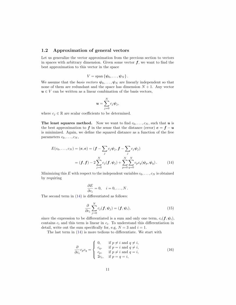
Less successful example. The next example concerns interpolating f(x) =|1 − 2x| on Ω = [0, 1] using Lagrange polynomials. Figure 9 shows a peculiareffect: the approximation starts to oscillate more and more as N grows. Thisnumerical artifact is not surprising when looking at the individual Lagrangepolynomials. Figure 10 shows two such polynomials, ψ2(x) and ψ7(x), both ofdegree 11 and computed from uniformly spaced points xxi
= i/11, i = 0, . . . , 11,marked with circles. We clearly see the property of Lagrange polynomials:ψ2(xi) = 0 and ψ7(xi) = 0 for all i, except ψ2(x2) = 1 and ψ7(x7) = 1. Themost striking feature, however, is the significant oscillation near the boundary.The reason is easy to understand: since we force the functions to zero at so manypoints, a polynomial of high degree is forced to oscillate between the points. Thephenomenon is named Runge’s phenomenon and you can read a more detailedexplanation on Wikipedia.
Remedy for strong oscillations. The oscillations can be reduced by a moreclever choice of interpolation points, called the Chebyshev nodes:
xi =1
2(a+ b) +
1
2(b− a) cos
(2i+ 1
2(N + 1)pi
), i = 0 . . . , N, (50)
on the interval Ω = [a, b]. Here is a flexible version of the Lagrange_polynomials_01function above, valid for any interval Ω = [a, b] and with the possibility to gener-ate both uniformly distributed points and Chebyshev nodes:
def Lagrange_polynomials(x, N, Omega, point_distribution=’uniform’):if point_distribution == ’uniform’:
if isinstance(x, sp.Symbol):h = sp.Rational(Omega[1] - Omega[0], N)
else:h = (Omega[1] - Omega[0])/float(N)
points = [Omega[0] + i*h for i in range(N+1)]elif point_distribution == ’Chebyshev’:
points = Chebyshev_nodes(Omega[0], Omega[1], N)psi = [Lagrange_polynomial(x, i, points) for i in range(N+1)]return psi, points
29

def Chebyshev_nodes(a, b, N):from math import cos, pireturn [0.5*(a+b) + 0.5*(b-a)*cos(float(2*i+1)/(2*N+1))*pi) \
for i in range(N+1)]
All the functions computing Lagrange polynomials listed above are found in themodule file Lagrange.py. Figure 11 shows the improvement of using Chebyshevnodes (compared with Figure 9). The reason is that the corresponding Lagrangepolynomials have much smaller oscillations as seen in Figure 12 (compare withFigure 10).
Another cure for undesired oscillation of higher-degree interpolating poly-nomials is to use lower-degree Lagrange polynomials on many small patches ofthe domain, which is the idea pursued in the finite element method. For in-stance, linear Lagrange polynomials on [0, 1/2] and [1/2, 1] would yield a perfectapproximation to f(x) = |1− 2x| on Ω = [0, 1] since f is piecewise linear.
0.0 0.2 0.4 0.6 0.8 1.0x
0.0
0.2
0.4
0.6
0.8
1.0Interpolation by Lagrange polynomials of degree 7
approximationexact
0.0 0.2 0.4 0.6 0.8 1.0x
4
3
2
1
0
1
2Interpolation by Lagrange polynomials of degree 14
approximationexact
Figure 9: Interpolation of an absolute value function by Lagrange polynomialsand uniformly distributed interpolation points: degree 7 (left) and 14 (right).
How does the least squares or projection methods work with Lagrangepolynomials? Unfortunately, sympy has problems integrating the f(x) = |1− 2x|function times a polynomial. Other choices of f(x) can also make the symbolicintegration fail. Therefore, we should extend the least_squares functionsuch that it falls back on numerical integration if the symbolic integration isunsuccessful. In the latter case, the returned value from sympy’s integrate
function is an object of type Integral. We can test on this type and utilizethe mpmath module in sympy to perform numerical integration of high precision.Here is the code:
def least_squares(f, psi, Omega):N = len(psi) - 1A = sp.zeros((N+1, N+1))b = sp.zeros((N+1, 1))x = sp.Symbol(’x’)for i in range(N+1):
for j in range(i, N+1):integrand = psi[i]*psi[j]I = sp.integrate(integrand, (x, Omega[0], Omega[1]))
30

0.0 0.2 0.4 0.6 0.8 1.010
8
6
4
2
0
2
4
6
ψ2
ψ7
Figure 10: Illustration of the oscillatory behavior of two Lagrange polynomialsbased on 12 uniformly spaced points (marked by circles).
0.0 0.2 0.4 0.6 0.8 1.0x
0.0
0.2
0.4
0.6
0.8
1.0
1.2Interpolation by Lagrange polynomials of degree 7
approximationexact
0.0 0.2 0.4 0.6 0.8 1.0x
0.2
0.0
0.2
0.4
0.6
0.8
1.0
1.2Interpolation by Lagrange polynomials of degree 14
approximationexact
Figure 11: Interpolation of an absolute value function by Lagrange polynomialsand Chebyshev nodes as interpolation points: degree 7 (left) and 14 (right).
if isinstance(I, sp.Integral):# Could not integrate symbolically, fallback# on numerical integration with mpmath.quadintegrand = sp.lambdify([x], integrand)I = sp.mpmath.quad(integrand, [Omega[0], Omega[1]])
A[i,j] = A[j,i] = Iintegrand = psi[i]*fI = sp.integrate(integrand, (x, Omega[0], Omega[1]))if isinstance(I, sp.Integral):
integrand = sp.lambdify([x], integrand)
31
0.0 0.2 0.4 0.6 0.8 1.010
8
6
4
2
0
2
4
6
ψ2
ψ7
Figure 12: Illustration of the less oscillatory behavior of two Lagrange polyno-mials based on 12 Chebyshev points (marked by circles).
I = sp.mpmath.quad(integrand, [Omega[0], Omega[1]])b[i,0] = I
c = A.LUsolve(b)u = 0for i in range(len(psi)):
u += c[i,0]*psi[i]return u
3 Finite element basis functions
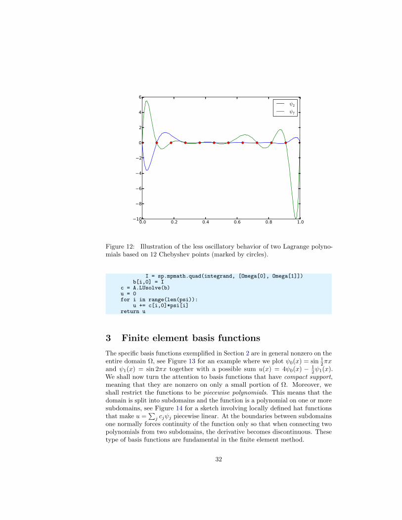
The specific basis functions exemplified in Section 2 are in general nonzero on theentire domain Ω, see Figure 13 for an example where we plot ψ0(x) = sin 1
2πxand ψ1(x) = sin 2πx together with a possible sum u(x) = 4ψ0(x) − 1
2ψ1(x).We shall now turn the attention to basis functions that have compact support,meaning that they are nonzero on only a small portion of Ω. Moreover, weshall restrict the functions to be piecewise polynomials. This means that thedomain is split into subdomains and the function is a polynomial on one or moresubdomains, see Figure 14 for a sketch involving locally defined hat functionsthat make u =
∑j cjψj piecewise linear. At the boundaries between subdomains
one normally forces continuity of the function only so that when connecting twopolynomials from two subdomains, the derivative becomes discontinuous. Thesetype of basis functions are fundamental in the finite element method.
32

0.0 0.5 1.0 1.5 2.0 2.5 3.0 3.5 4.0
4
2
0
2
4ψ0
ψ1
u=4ψ0−12ψ1
Figure 13: A function resulting from adding two sine basis functions.
We first introduce the concepts of elements and nodes in a simplistic fashionas often met in the literature. Later, we shall generalize the concept of anelement, which is a necessary step to treat a wider class of approximations withinthe family of finite element methods. The generalization is also compatible withthe concepts used in the FEniCS finite element software.
3.1 Elements and nodes
Let us divide the interval Ω on which f and u are defined into non-overlappingsubintervals Ω(e), e = 0, . . . , Ne:
Ω = Ω(0) ∪ · · · ∪ Ω(Ne) . (51)
We shall for now refer to Ω(e) as an element, having number e. On each elementwe introduce a set of points called nodes. For now we assume that the nodesare uniformly spaced throughout the element and that the boundary pointsof the elements are also nodes. The nodes are given numbers both within anelement and in the global domain. These are referred to as local and global nodenumbers, respectively. Figure 15 shows element boundaries with small verticallines, nodes as small disks, element numbers in circles, and global node numbersunder the nodes.
Nodes and elements uniquely define a finite element mesh, which is ourdiscrete representation of the domain in the computations. A common special
33

0.0 0.5 1.0 1.5 2.0 2.5 3.0 3.5 4.00
1
2
3
4
5
6
7
8
9
ϕ0 ϕ1 ϕ2
u
Figure 14: A function resulting from adding three local piecewise linear (hat)functions.
0 2 4 61.5
1.0
0.5
0.0
0.5
1.0
1.5
2.0
2.5
543210
x
Ω(4)Ω(0) Ω(1) Ω(2) Ω(3)
Figure 15: Finite element mesh with 5 elements and 6 nodes.
case is that of a uniformly partitioned mesh where each element has the samelength and the distance between nodes is constant.
Example. On Ω = [0, 1] we may introduce two elements, Ω(0) = [0, 0.4] andΩ(1) = [0.4, 1]. Furthermore, let us introduce three nodes per element, equallyspaced within each element. Figure 16 shows the mesh. The three nodes inelement number 0 are x0 = 0, x1 = 0.2, and x2 = 0.4. The local and global nodenumbers are here equal. In element number 1, we have the local nodes x0 = 0.4,
34

x1 = 0.7, and x2 = 1 and the corresponding global nodes x2 = 0.4, x3 = 0.7,and x4 = 1. Note that the global node x2 = 0.4 is shared by the two elements.
0.2 0.0 0.2 0.4 0.6 0.8 1.0 1.2
0.2
0.1
0.0
0.1
0.2
0.3
0.4
0.5
43210
x
Ω(0) Ω(1)
Figure 16: Finite element mesh with 2 elements and 5 nodes.
For the purpose of implementation, we introduce two lists or arrays: nodesfor storing the coordinates of the nodes, with the global node numbers as indices,and elements for holding the global node numbers in each element, with thelocal node numbers as indices. The nodes and elements lists for the samplemesh above take the form
nodes = [0, 0.2, 0.4, 0.7, 1]elements = [[0, 1, 2], [2, 3, 4]]
Looking up the coordinate of local node number 2 in element 1 is here done bynodes[elements[1][2]] (recall that nodes and elements start their numberingat 0).
The numbering of elements and nodes does not need to be regular. Figure 17shows and example corresponding to
nodes = [1.5, 5.5, 4.2, 0.3, 2.2, 3.1]elements = [[2, 1], [4, 5], [0, 4], [3, 0], [5, 2]]
3.2 The basis functions
Construction principles. Finite element basis functions are in this text rec-ognized by the notation ϕi(x), where the index now in the beginning correspondsto a global node number. In the current approximation problem we shall simplytake ψi = ϕi.
Let i be the global node number corresponding to local node r in elementnumber e. The finite element basis functions ϕi are now defined as follows.
35

0 1 2 3 4 5 6 71.5
1.0
0.5
0.0
0.5
1.0
1.5
2.0
2.5
543 2 10
x
Ω(4) Ω(0)Ω(1)Ω(2)Ω(3)
Figure 17: Example on irregular numbering of elements and nodes.
• If local node number r is not on the boundary of the element, take ϕi(x)to be the Lagrange polynomial that is 1 at the local node number r andzero at all other nodes in the element. On all other elements, ϕi = 0.
• If local node number r is on the boundary of the element, let ϕi be madeup of the Lagrange polynomial over element e that is 1 at node i, combinedwith the Lagrange polynomial over element e+ 1 that is also 1 at node i.On all other elements, ϕi = 0.
A visual impression of three such basis functions are given in Figure 18.
Properties of ϕi. The construction of basis functions according to the princi-ples above lead to two important properties of ϕi(x). First,
ϕi(xj) = δij , δij =
1, i = j,0, i 6= j,
(52)
when xj is a node in the mesh with global node number j. The result ϕi(xj) = δijarises because the Lagrange polynomials are constructed to have exactly thisproperty. The property also implies a convenient interpretation of ci as the valueof u at node i. To show this, we expand u in the usual way as
∑j cjψj and
choose ψi = ϕi:
u(xi) =∑j∈Is
cjψj(xi) =∑j∈Is
cjϕj(xi) = ciϕi(xi) = ci .
Because of this interpretation, the coefficient ci is by many named ui or Ui.Second, ϕi(x) is mostly zero throughout the domain:
• ϕi(x) 6= 0 only on those elements that contain global node i,
• ϕi(x)ϕj(x) 6= 0 if and only if i and j are global node numbers in the sameelement.
36

0.0 0.2 0.4 0.6 0.8 1.00.2
0.0
0.2
0.4
0.6
0.8
1.0 ϕ2
ϕ3
ϕ4
Figure 18: Illustration of the piecewise quadratic basis functions associatedwith nodes in element 1.
Since Ai,j is the integral of ϕiϕj it means that most of the elements in thecoefficient matrix will be zero. We will come back to these properties and usethem actively in computations to save memory and CPU time.
We let each element have d+1 nodes, resulting in local Lagrange polynomialsof degree d. It is not a requirement to have the same d value in each element,but for now we will assume so.
3.3 Example on piecewise quadratic finite element func-tions
Figure 18 illustrates how piecewise quadratic basis functions can look like (d = 2).We work with the domain Ω = [0, 1] divided into four equal-sized elements, eachhaving three nodes. The nodes and elements lists in this particular examplebecome
nodes = [0, 0.125, 0.25, 0.375, 0.5, 0.625, 0.75, 0.875, 1.0]elements = [[0, 1, 2], [2, 3, 4], [4, 5, 6], [6, 7, 8]]
Figure 19 sketches the mesh and the numbering. Nodes are marked with circleson the x axis and element boundaries are marked with vertical dashed lines inFigure 18.
Let us explain in detail how the basis functions are constructed accordingto the principles. Consider element number 1 in Figure 18, Ω(1) = [0.25, 0.5],
37

0.2 0.0 0.2 0.4 0.6 0.8 1.0 1.2
0.2
0.1
0.0
0.1
0.2
0.3
0.4
0.5
43210
x
Ω(0) Ω(1)
Figure 19: Sketch of mesh with 4 elements and 3 nodes per element.
with local nodes 0, 1, and 2 corresponding to global nodes 2, 3, and 4. Thecoordinates of these nodes are 0.25, 0.375, and 0.5, respectively. We define threeLagrange polynomials on this element:
1. The polynomial that is 1 at local node 1 (x = 0.375, global node 3) makesup the basis function ϕ3(x) over this element, with ϕ3(x) = 0 outside theelement.
2. The Lagrange polynomial that is 1 at local node 0 is the ”right part”of the global basis function ϕ2(x). The ”left part” of ϕ2(x) consists ofa Lagrange polynomial associated with local node 2 in the neighboringelement Ω(0) = [0, 0.25].
3. Finally, the polynomial that is 1 at local node 2 (global node 4) is the ”leftpart” of the global basis function ϕ4(x). The ”right part” comes from theLagrange polynomial that is 1 at local node 0 in the neighboring elementΩ(2) = [0.5, 0.75].
As mentioned earlier, any global basis function ϕi(x) is zero on elements thatdo not contain the node with global node number i.
The other global functions associated with internal nodes, ϕ1, ϕ5, and ϕ7, areall of the same shape as the drawn ϕ3, while the global basis functions associatedwith shared nodes also have the same shape, provided the elements are of thesame length.
3.4 Example on piecewise linear finite element functions
Figure 20 shows piecewise linear basis functions (d = 1). Also here we havefour elements on Ω = [0, 1]. Consider the element Ω(1) = [0.25, 0.5]. Now thereare no internal nodes in the elements so that all basis functions are associatedwith nodes at the element boundaries and hence made up of two Lagrange
38

0.0 0.2 0.4 0.6 0.8 1.0
0.0
0.2
0.4
0.6
0.8
1.0ϕ1
ϕ2
Figure 20: Illustration of the piecewise linear basis functions associated withnodes in element 1.
polynomials from neighboring elements. For example, ϕ1(x) results from theLagrange polynomial in element 0 that is 1 at local node 1 and 0 at local node0, combined with the Lagrange polynomial in element 1 that is 1 at local node 0and 0 at local node 1. The other basis functions are constructed similarly.
Explicit mathematical formulas are needed for ϕi(x) in computations. In thepiecewise linear case, one can show that
ϕi(x) =
0, x < xi−1,(x− xi−1)/(xi − xi−1), xi−1 ≤ x < xi,1− (x− xi)/(xi+1 − xi), xi ≤ x < xi+1,0, x ≥ xi+1 .
(53)
Here, xj , j = i− 1, i, i+ 1, denotes the coordinate of node j. For elements ofequal length h the formulas can be simplified to
ϕi(x) =
0, x < xi−1,(x− xi−1)/h, xi−1 ≤ x < xi,1− (x− xi)/h, xi ≤ x < xi+1,0, x ≥ xi+1
(54)
39

3.5 Example on piecewise cubic finite element basis func-tions
Piecewise cubic basis functions can be defined by introducing four nodes perelement. Figure 21 shows examples on ϕi(x), i = 3, 4, 5, 6, associated withelement number 1. Note that ϕ4 and ϕ5 are nonzero on element number 1, whileϕ3 and ϕ6 are made up of Lagrange polynomials on two neighboring elements.
0.0 0.2 0.4 0.6 0.8 1.00.4
0.2
0.0
0.2
0.4
0.6
0.8
1.0
Figure 21: Illustration of the piecewise cubic basis functions associated withnodes in element 1.
We see that all the piecewise linear basis functions have the same ”hat” shape.They are naturally referred to as hat functions, also called chapeau functions.The piecewise quadratic functions in Figure 18 are seen to be of two types.”Rounded hats” associated with internal nodes in the elements and some more”sombrero” shaped hats associated with element boundary nodes. Higher-orderbasis functions also have hat-like shapes, but the functions have pronouncedoscillations in addition, as illustrated in Figure 21.
A common terminology is to speak about linear elements as elements with twolocal nodes associated with piecewise linear basis functions. Similarly, quadraticelements and cubic elements refer to piecewise quadratic or cubic functionsover elements with three or four local nodes, respectively. Alternative names,frequently used later, are P1 elements for linear elements, P2 for quadraticelements, and so forth: Pd signifies degree d of the polynomial basis functions.
40

3.6 Calculating the linear system
The elements in the coefficient matrix and right-hand side are given by theformulas (27) and (28), but now the choice of ψi is ϕi. Consider P1 elementswhere ϕi(x) piecewise linear. Nodes and elements numbered consecutively fromleft to right in a uniformly partitioned mesh imply the nodes
xi = ih, i = 0, . . . , N,
and the elements
Ω(i) = [xi, xi+1] = [ih, (i+ 1)h], i = 0, . . . , Ne = N − 1 . (55)
We have in this case N elements and N + 1 nodes, and Ω = [x0, xN ]. Theformula for ϕi(x) is given by (54) and a graphical illustration is provided inFigures 20 and 23. First we clearly see from the figures the very importantproperty ϕi(x)ϕj(x) 6= 0 if and only if j = i − 1, j = i, or j = i + 1, oralternatively expressed, if and only if i and j are nodes in the same element.Otherwise, ϕi and ϕj are too distant to have an overlap and consequently theirproduct vanishes.
0 2 4 61.5
1.0
0.5
0.0
0.5
1.0
1.5
2.0
2.5
543210
x
Ω(4)Ω(0) Ω(1) Ω(2) Ω(3)
φ2 φ3
Figure 22: Illustration of the piecewise linear basis functions corresponding toglobal node 2 and 3.
Calculating a specific matrix entry. Let us calculate the specific matrixentry A2,3 =
∫Ωϕ2ϕ3 dx. Figure 22 shows how ϕ2 and ϕ3 look like. We realize
from this figure that the product ϕ2ϕ3 6= 0 only over element 2, which containsnode 2 and 3. The particular formulas for ϕ2(x) and ϕ3(x) on [x2, x3] are foundfrom (54). The function ϕ3 has positive slope over [x2, x3] and corresponds tothe interval [xi−1, xi] in (54). With i = 3 we get
ϕ3(x) = (x− x2)/h,
while ϕ2(x) has negative slope over [x2, x3] and corresponds to setting i = 2 in(54),
41

ϕ2(x) = 1− (x− x2)/h .
We can now easily integrate,
A2,3 =
∫Ω
ϕ2ϕ3 dx =
∫ x3
x2
(1− x− x2
h
)x− x2
hdx =
h
6.
The diagonal entry in the coefficient matrix becomes
A2,2 =
∫ x2
x1
(x− x1
h
)2
dx+
∫ x3
x2
(1− x− x2
h
)2
dx =h
3.
The entry A2,1 has an the integral that is geometrically similar to the situationin Figure 22, so we get A2,1 = h/6.
Calculating a general row in the matrix. We can now generalize thecalculation of matrix entries to a general row number i. The entry Ai,i−1 =∫
Ωϕiϕi−1 dx involves hat functions as depicted in Figure 23. Since the integral
is geometrically identical to the situation with specific nodes 2 and 3, we realizethat Ai,i−1 = Ai,i+1 = h/6 and Ai,i = 2h/3. However, we can compute theintegral directly too:
Ai,i−1 =
∫Ω
ϕiϕi−1 dx
=
∫ xi−1
xi−2
ϕiϕi−1 dx︸ ︷︷ ︸ϕi=0
+
∫ xi
xi−1
ϕiϕi−1 dx+
∫ xi+1
xi
ϕiϕi−1 dx︸ ︷︷ ︸ϕi−1=0
=
∫ xi
xi−1
(x− xih
)︸ ︷︷ ︸
ϕi(x)
(1− x− xi−1
h
)︸ ︷︷ ︸
ϕi−1(x)
dx =h
6.
The particular formulas for ϕi−1(x) and ϕi(x) on [xi−1, xi] are found from(54): ϕi is the linear function with positive slope, corresponding to the interval[xi−1, xi] in (54), while φi−1 has a negative slope so the definition in interval[xi, xi+1] in (54) must be used. (The appearance of i in (54) and the integralmight be confusing, as we speak about two different i indices.)
The first and last row of the coefficient matrix lead to slightly differentintegrals:
A0,0 =
∫Ω
ϕ20 dx =
∫ x1
x0
(1− x− x0
h
)2
dx =h
3.
Similarly, AN,N involves an integral over only one element and equals hence h/3.The general formula for bi, see Figure 24, is now easy to set up
42

0 2 4 61.5
1.0
0.5
0.0
0.5
1.0
1.5
2.0
2.5
i+1ii−1i−2
x
φi−1 φi
Figure 23: Illustration of two neighboring linear (hat) functions with generalnode numbers.
0 2 4 61.5
1.0
0.5
0.0
0.5
1.0
1.5
2.0
2.5
i+1ii−1i−2
x
φi f(x)
Figure 24: Right-hand side integral with the product of a basis function andthe given function to approximate.
bi =
∫Ω
ϕi(x)f(x) dx =
∫ xi
xi−1
x− xi−1
hf(x) dx+
∫ xi+1
xi
(1− x− xi
h
)f(x) dx .
(56)We need a specific f(x) function to compute these integrals. With two equal-sizedelements in Ω = [0, 1] and f(x) = x(1− x), one gets
A =h
6
2 1 01 4 10 1 2
, b =h2
12
2− 3h12− 14h10− 17h
.
The solution becomes
c0 =h2
6, c1 = h− 5
6h2, c2 = 2h− 23
6h2 .
The resulting function
43

u(x) = c0ϕ0(x) + c1ϕ1(x) + c2ϕ2(x)
is displayed in Figure 25 (left). Doubling the number of elements to four leadsto the improved approximation in the right part of Figure 25.
0.0 0.2 0.4 0.6 0.8 1.00.00
0.05
0.10
0.15
0.20
0.25
0.30
uf
0.0 0.2 0.4 0.6 0.8 1.00.00
0.05
0.10
0.15
0.20
0.25
0.30
uf
Figure 25: Least squares approximation of a parabola using 2 (left) and 4(right) P1 elements.
3.7 Assembly of elementwise computations
The integrals above are naturally split into integrals over individual elementssince the formulas change with the elements. This idea of splitting the integralis fundamental in all practical implementations of the finite element method.
Let us split the integral over Ω into a sum of contributions from each element:
Ai,j =
∫Ω
ϕiϕj dx =∑e
A(e)i,j , A
(e)i,j =
∫Ω(e)
ϕiϕj dx . (57)
Now, A(e)i,j 6= 0 if and only if i and j are nodes in element e. Introduce i = q(e, r)
as the mapping of local node number r in element e to the global node number i.This is just a short mathematical notation for the expression i=elements[e][r]
in a program. Let r and s be the local node numbers corresponding to the globalnode numbers i = q(e, r) and j = q(e, s). With d nodes per element, all the
nonzero elements in A(e)i,j arise from the integrals involving basis functions with
indices corresponding to the global node numbers in element number e:∫Ω(e)
ϕq(e,r)ϕq(e,s) dx, r, s = 0, . . . , d .
These contributions can be collected in a (d + 1) × (d + 1) matrix known asthe element matrix. Let Id = 0, . . . , d be the valid indices of r and s. Weintroduce the notation
A(e) = A(e)r,s, r, s ∈ Id,
44

for the element matrix. For the case d = 2 we have
A(e) =
A(e)0,0 A
(e)0,1 A
(e)0,2
A(e)1,0 A
(e)1,1 A
(e)1,2
A(e)2,0 A
(e)2,1 A
(e)2,2
.Given the numbers A
(e)r,s , we should according to (57) add the contributions to
the global coefficient matrix by
Aq(e,r),q(e,s) := Aq(e,r),q(e,s) + A(e)r,s , r, s ∈ Id . (58)
This process of adding in elementwise contributions to the global matrix is calledfinite element assembly or simply assembly. Figure 26 illustrates how elementmatrices for elements with two nodes are added into the global matrix. Morespecifically, the figure shows how the element matrix associated with elements 1and 2 assembled, assuming that global nodes are numbered from left to right inthe domain. With regularly numbered P3 elements, where the element matriceshave size 4× 4, the assembly of elements 1 and 2 are sketched in Figure 27.
Figure 26: Illustration of matrix assembly: regularly numbered P1 elements.
After assembly of element matrices corresponding to regularly numberedelements and nodes are understood, it is wise to study the assembly process forirregularly numbered elements and nodes. Figure 17 shows a mesh where theelements array, or q(e, r) mapping in mathematical notation, is given as
45

Figure 27: Illustration of matrix assembly: regularly numbered P3 elements.
elements = [[2, 1], [4, 5], [0, 4], [3, 0], [5, 2]]
The associated assembly of element matrices 1 and 2 is sketched in Figure 28.These three assembly processes can also be animated.The right-hand side of the linear system is also computed elementwise:
bi =
∫Ω
f(x)ϕi(x) dx =∑e
b(e)i , b
(e)i =
∫Ω(e)
f(x)ϕi(x) dx . (59)
We observe that b(e)i 6= 0 if and only if global node i is a node in element e.
With d nodes per element we can collect the d+ 1 nonzero contributions b(e)i ,
for i = q(e, r), r ∈ Id, in an element vector
b(e)r = b(e)r , r ∈ Id .
These contributions are added to the global right-hand side by an assemblyprocess similar to that for the element matrices:
46

Figure 28: Illustration of matrix assembly: irregularly numbered P1 elements.
bq(e,r) := bq(e,r) + b(e)r , r ∈ Id . (60)
3.8 Mapping to a reference element
Instead of computing the integrals
A(e)r,s =
∫Ω(e)
ϕq(e,r)(x)ϕq(e,s)(x) dx
over some element Ω(e) = [xL, xR], it is convenient to map the element domain[xL, xR] to a standardized reference element domain [−1, 1]. (We have nowintroduced xL and xR as the left and right boundary points of an arbitraryelement. With a natural, regular numbering of nodes and elements from left toright through the domain, we have xL = xe and xR = xe+1 for P1 elements.)
Let X ∈ [−1, 1] be the coordinate in the reference element. A linear or affinemapping from X to x reads
x =1
2(xL + xR) +
1
2(xR − xL)X . (61)
This relation can alternatively be expressed by
x = xm +1
2hX, (62)
47

where we have introduced the element midpoint xm = (xL + xR)/2 and theelement length h = xR − xL.
Integrating on the reference element is a matter of just changing the integra-tion variable from x to X. Let
ϕr(X) = ϕq(e,r)(x(X)) (63)
be the basis function associated with local node number r in the referenceelement. The integral transformation reads
A(e)r,s =
∫Ω(e)
ϕq(e,r)(x)ϕq(e,s)(x) dx =
∫ 1
−1
ϕr(X)ϕs(X)dx
dXdX . (64)
The stretch factor dx/dX between the x and X coordinates becomes the deter-minant of the Jacobian matrix of the mapping between the coordinate systemsin 2D and 3D. To obtain a uniform notation for 1D, 2D, and 3D problems wetherefore replace dx/dX by det J already now. In 1D, det J = dx/dX = h/2.The integration over the reference element is then written as
A(e)r,s =
∫ 1
−1
ϕr(X)ϕs(X) detJ dX . (65)
The corresponding formula for the element vector entries becomes
b(e)r =
∫Ω(e)
f(x)ϕq(e,r)(x)dx =
∫ 1
−1
f(x(X))ϕr(X) detJ dX . (66)
Since we from now on will work in the reference element, we need explicitmathematical formulas for the basis functions ϕi(x) in the reference elementonly, i.e., we only need to specify formulas for ϕr(X). This is a very convenientsimplification compared to specifying piecewise polynomials in the physicaldomain.
The ϕr(x) functions are simply the Lagrange polynomials defined throughthe local nodes in the reference element. For d = 1 and two nodes per element,we have the linear Lagrange polynomials
ϕ0(X) =1
2(1−X) (67)
ϕ1(X) =1
2(1 +X) (68)
Quadratic polynomials, d = 2, have the formulas
ϕ0(X) =1
2(X − 1)X (69)
ϕ1(X) = 1−X2 (70)
ϕ2(X) =1
2(X + 1)X (71)
48

In general,
ϕr(X) =
d∏s=0,s6=r
X −X(s)
X(r) −X(s), (72)
where X(0), . . . , X(d) are the coordinates of the local nodes in the referenceelement. These are normally uniformly spaced: X(r) = −1 + 2r/d, r ∈ Id.
Why reference elements?
The great advantage of using reference elements is that the formulas forthe basis functions, ϕr(X), are the same for all elements and independentof the element geometry (length and location in the mesh). The geometricinformation is ”factored out” in the simple mapping formula and the asso-ciated det J quantity, but this information is (here taken as) the same forelement types. Also, the integration domain is the same for all elements.
3.9 Example: Integration over a reference element
To illustrate the concepts from the previous section in a specific example, wenow consider calculation of the element matrix and vector for a specific choiceof d and f(x). A simple choice is d = 1 (P1 elements) and f(x) = x(1 − x)
on Ω = [0, 1]. We have the general expressions (65) and (66) for A(e)r,s and b
(e)r .
Writing these out for the choices (67) and (68), and using that det J = h/2, wecan do the following calculations of the element matrix entries:
A(e)0,0 =
∫ 1
−1
ϕ0(X)ϕ0(X)h
2dX
=
∫ 1
−1
1
2(1−X)
1
2(1−X)
h
2dX =
h
8
∫ 1
−1
(1−X)2dX =h
3, (73)
A(e)1,0 =
∫ 1
−1
ϕ1(X)ϕ0(X)h
2dX
=
∫ 1
−1
1
2(1 +X)
1
2(1−X)
h
2dX =
h
8
∫ 1
−1
(1−X2)dX =h
6, (74)
A(e)0,1 = A
(e)1,0, (75)
A(e)1,1 =
∫ 1
−1
ϕ1(X)ϕ1(X)h
2dX
=
∫ 1
−1
1
2(1 +X)
1
2(1 +X)
h
2dX =
h
8
∫ 1
−1
(1 +X)2dX =h
3. (76)
The corresponding entries in the element vector becomes
49

b(e)0 =
∫ 1
−1
f(x(X))ϕ0(X)h
2dX
=
∫ 1
−1
(xm +1
2hX)(1− (xm +
1
2hX))
1
2(1−X)
h
2dX
= − 1
24h3 +
1
6h2xm −
1
12h2 − 1
2hx2
m +1
2hxm (77)
b(e)1 =
∫ 1
−1
f(x(X))ϕ1(X)h
2dX
=
∫ 1
−1
(xm +1
2hX)(1− (xm +
1
2hX))
1
2(1 +X)
h
2dX
= − 1
24h3 − 1
6h2xm +
1
12h2 − 1
2hx2
m +1
2hxm . (78)
In the last two expressions we have used the element midpoint xm.Integration of lower-degree polynomials above is tedious, and higher-degree
polynomials involve very much more algebra, but sympy may help. For example,we can easily calculate (73), (73), and (77) by
>>> import sympy as sp>>> x, x_m, h, X = sp.symbols(’x x_m h X’)>>> sp.integrate(h/8*(1-X)**2, (X, -1, 1))h/3>>> sp.integrate(h/8*(1+X)*(1-X), (X, -1, 1))h/6>>> x = x_m + h/2*X>>> b_0 = sp.integrate(h/4*x*(1-x)*(1-X), (X, -1, 1))>>> print b_0-h**3/24 + h**2*x_m/6 - h**2/12 - h*x_m**2/2 + h*x_m/2
For inclusion of formulas in documents (like the present one), sympy can printexpressions in LATEX format:
>>> print sp.latex(b_0, mode=’plain’)- \frac124 h^3 + \frac16 h^2 x_m- \frac112 h^2 - \half h x_m^2+ \half h x_m
4 Implementation
Based on the experience from the previous example, it makes sense to writesome code to automate the analytical integration process for any choice of finiteelement basis functions. In addition, we can automate the assembly processand linear system solution. Appropriate functions for this purpose documentall details of all steps in the finite element computations and can found in themodule file fe_approx1D.py. The key steps in the computational machinery arenow explained in detail in terms of code and text.
50

4.1 Integration
First we need a Python function for defining ϕr(X) in terms of a Lagrangepolynomial of degree d:
import sympy as spimport numpy as np
def phi_r(r, X, d):if isinstance(X, sp.Symbol):
h = sp.Rational(1, d) # node spacingnodes = [2*i*h - 1 for i in range(d+1)]
else:# assume X is numeric: use floats for nodesnodes = np.linspace(-1, 1, d+1)
return Lagrange_polynomial(X, r, nodes)
def Lagrange_polynomial(x, i, points):p = 1for k in range(len(points)):
if k != i:p *= (x - points[k])/(points[i] - points[k])
return p
Observe how we construct the phi_r function to be a symbolic expression forϕr(X) if X is a Symbol object from sympy. Otherwise, we assume that X is a float
object and compute the corresponding floating-point value of ϕr(X). Recall thatthe Lagrange_polynomial function, here simply copied from Section 2.7, workswith both symbolic and numeric variables.
The complete basis ϕ0(X), . . . , ϕd(X) on the reference element, representedas a list of symbolic expressions, is constructed by
def basis(d=1):X = sp.Symbol(’X’)phi = [phi_r(r, X, d) for r in range(d+1)]return phi
Now we are in a position to write the function for computing the element matrix:
def element_matrix(phi, Omega_e, symbolic=True):n = len(phi)A_e = sp.zeros((n, n))X = sp.Symbol(’X’)if symbolic:
h = sp.Symbol(’h’)else:
h = Omega_e[1] - Omega_e[0]detJ = h/2 # dx/dXfor r in range(n):
for s in range(r, n):A_e[r,s] = sp.integrate(phi[r]*phi[s]*detJ, (X, -1, 1))A_e[s,r] = A_e[r,s]
return A_e
In the symbolic case (symbolic is True), we introduce the element length asa symbol h in the computations. Otherwise, the real numerical value of the
51

element interval Omega_e is used and the final matrix elements are numbers, notsymbols. This functionality can be demonstrated:
>>> from fe_approx1D import *>>> phi = basis(d=1)>>> phi[1/2 - X/2, 1/2 + X/2]>>> element_matrix(phi, Omega_e=[0.1, 0.2], symbolic=True)[h/3, h/6][h/6, h/3]>>> element_matrix(phi, Omega_e=[0.1, 0.2], symbolic=False)[0.0333333333333333, 0.0166666666666667][0.0166666666666667, 0.0333333333333333]
The computation of the element vector is done by a similar procedure:
def element_vector(f, phi, Omega_e, symbolic=True):n = len(phi)b_e = sp.zeros((n, 1))# Make f a function of XX = sp.Symbol(’X’)if symbolic:
h = sp.Symbol(’h’)else:
h = Omega_e[1] - Omega_e[0]x = (Omega_e[0] + Omega_e[1])/2 + h/2*X # mappingf = f.subs(’x’, x) # substitute mapping formula for xdetJ = h/2 # dx/dXfor r in range(n):
b_e[r] = sp.integrate(f*phi[r]*detJ, (X, -1, 1))return b_e
Here we need to replace the symbol x in the expression for f by the mapping
formula such that f can be integrated in terms of X, cf. the formula b(e)r =∫ 1
−1f(x(X))ϕr(X)h2dX.The integration in the element matrix function involves only products of
polynomials, which sympy can easily deal with, but for the right-hand side sympy
may face difficulties with certain types of expressions f. The result of the integralis then an Integral object and not a number or expression as when symbolicintegration is successful. It may therefore be wise to introduce a fallback onnumerical integration. The symbolic integration can also take much time beforean unsuccessful conclusion so we may also introduce a parameter symbolic andset it to False to avoid symbolic integration:
def element_vector(f, phi, Omega_e, symbolic=True):...if symbolic:
I = sp.integrate(f*phi[r]*detJ, (X, -1, 1))if not symbolic or isinstance(I, sp.Integral):
h = Omega_e[1] - Omega_e[0] # Ensure h is numericaldetJ = h/2integrand = sp.lambdify([X], f*phi[r]*detJ)I = sp.mpmath.quad(integrand, [-1, 1])
b_e[r] = I...
52

Numerical integration requires that the symbolic integrand is converted to a plainPython function (integrand) and that the element length h is a real number.
4.2 Linear system assembly and solution
The complete algorithm for computing and assembling the elementwise contribu-tions takes the following form
def assemble(nodes, elements, phi, f, symbolic=True):N_n, N_e = len(nodes), len(elements)if symbolic:
A = sp.zeros((N_n, N_n))b = sp.zeros((N_n, 1)) # note: (N_n, 1) matrix
else:A = np.zeros((N_n, N_n))b = np.zeros(N_n)
for e in range(N_e):Omega_e = [nodes[elements[e][0]], nodes[elements[e][-1]]]
A_e = element_matrix(phi, Omega_e, symbolic)b_e = element_vector(f, phi, Omega_e, symbolic)
for r in range(len(elements[e])):for s in range(len(elements[e])):
A[elements[e][r],elements[e][s]] += A_e[r,s]b[elements[e][r]] += b_e[r]
return A, b
The nodes and elements variables represent the finite element mesh as explainedearlier.
Given the coefficient matrix A and the right-hand side b, we can computethe coefficients cii∈Is in the expansion u(x) =
∑j cjϕj as the solution vector
c of the linear system:
if symbolic:c = A.LUsolve(b)
else:c = np.linalg.solve(A, b)
When A and b are sympy arrays, the solution procedure implied by A.LUsolve issymbolic. Otherwise, A and b are numpy arrays and a standard numerical solveris called. The symbolic version is suited for small problems only (small N values)since the calculation time becomes prohibitively large otherwise. Normally, thesymbolic integration will be more time consuming in small problems than thesymbolic solution of the linear system.
4.3 Example on computing symbolic approximations
We can exemplify the use of assemble on the computational case from Section 3.6with two P1 elements (linear basis functions) on the domain Ω = [0, 1]. Let usfirst work with a symbolic element length:
53

>>> h, x = sp.symbols(’h x’)>>> nodes = [0, h, 2*h]>>> elements = [[0, 1], [1, 2]]>>> phi = basis(d=1)>>> f = x*(1-x)>>> A, b = assemble(nodes, elements, phi, f, symbolic=True)>>> A[h/3, h/6, 0][h/6, 2*h/3, h/6][ 0, h/6, h/3]>>> b[ h**2/6 - h**3/12][ h**2 - 7*h**3/6][5*h**2/6 - 17*h**3/12]>>> c = A.LUsolve(b)>>> c[ h**2/6][12*(7*h**2/12 - 35*h**3/72)/(7*h)][ 7*(4*h**2/7 - 23*h**3/21)/(2*h)]
4.4 Comparison with finite elements and interpolation/-collocation
We may, for comparison, compute the c vector corresponding to an interpola-tion/collocation method with finite element basis functions. Choosing the nodesas points, the principle is
u(xi) =∑j∈Is
cjϕj(xi) = f(xi), i ∈ Is .
The coefficient matrix Ai,j = ϕj(xi) becomes the identity matrix because basisfunction number j vanishes at all nodes, except node j: ϕj(xi = δij . Therefore,ci = f(xi.
The associated sympy calculations are
>>> fn = sp.lambdify([x], f)>>> c = [fn(xc) for xc in nodes]>>> c[0, h*(1 - h), 2*h*(1 - 2*h)]
These expressions are much simpler than those based on least squares or projec-tion in combination with finite element basis functions.
4.5 Example on computing numerical approximations
The numerical computations corresponding to the symbolic ones in Section 4.3,and still done by sympy and the assemble function, go as follows:
>>> nodes = [0, 0.5, 1]>>> elements = [[0, 1], [1, 2]]>>> phi = basis(d=1)>>> x = sp.Symbol(’x’)
54

>>> f = x*(1-x)>>> A, b = assemble(nodes, elements, phi, f, symbolic=False)>>> A[ 0.166666666666667, 0.0833333333333333, 0][0.0833333333333333, 0.333333333333333, 0.0833333333333333][ 0, 0.0833333333333333, 0.166666666666667]>>> b[ 0.03125][0.104166666666667][ 0.03125]>>> c = A.LUsolve(b)>>> c[0.0416666666666666][ 0.291666666666667][0.0416666666666666]
The fe_approx1D module contains functions for generating the nodes andelements lists for equal-sized elements with any number of nodes per element.The coordinates in nodes can be expressed either through the element lengthsymbol h (symbolic=True) or by real numbers (symbolic=False):
nodes, elements = mesh_uniform(N_e=10, d=3, Omega=[0,1],symbolic=True)
There is also a function
def approximate(f, symbolic=False, d=1, N_e=4, filename=’tmp.pdf’):
which computes a mesh with N_e elements, basis functions of degree d, andapproximates a given symbolic expression f by a finite element expansion u(x) =∑j cjϕj(x). When symbolic is False, u(x) =
∑j cjϕj(x) can be computed at
a (large) number of points and plotted together with f(x). The construction of upoints from the solution vector c is done elementwise by evaluating
∑r crϕr(X)
at a (large) number of points in each element in the local coordinate system,and the discrete (x, u) values on each element are stored in separate arrays thatare finally concatenated to form a global array for x and for u. The details arefound in the u_glob function in fe_approx1D.py.
4.6 The structure of the coefficient matrix
Let us first see how the global matrix looks like if we assemble symbolic elementmatrices, expressed in terms of h, from several elements:
>>> d=1; N_e=8; Omega=[0,1] # 8 linear elements on [0,1]>>> phi = basis(d)>>> f = x*(1-x)>>> nodes, elements = mesh_symbolic(N_e, d, Omega)>>> A, b = assemble(nodes, elements, phi, f, symbolic=True)>>> A[h/3, h/6, 0, 0, 0, 0, 0, 0, 0][h/6, 2*h/3, h/6, 0, 0, 0, 0, 0, 0][ 0, h/6, 2*h/3, h/6, 0, 0, 0, 0, 0]
55

[ 0, 0, h/6, 2*h/3, h/6, 0, 0, 0, 0][ 0, 0, 0, h/6, 2*h/3, h/6, 0, 0, 0][ 0, 0, 0, 0, h/6, 2*h/3, h/6, 0, 0][ 0, 0, 0, 0, 0, h/6, 2*h/3, h/6, 0][ 0, 0, 0, 0, 0, 0, h/6, 2*h/3, h/6][ 0, 0, 0, 0, 0, 0, 0, h/6, h/3]
The reader is encouraged to assemble the element matrices by hand and verifythis result, as this exercise will give a hands-on understanding of what theassembly is about. In general we have a coefficient matrix that is tridiagonal:
A =h
6
2 1 0 · · · · · · · · · · · · · · · 0
1 4 1. . .
...
0 1 4 1. . .
......
. . .. . .
. . . 0...
.... . .
. . .. . .
. . .. . .
...... 0 1 4 1
. . ....
.... . .
. . .. . .
. . . 0...
. . . 1 4 10 · · · · · · · · · · · · · · · 0 1 2
(79)
The structure of the right-hand side is more difficult to reveal since it involvesan assembly of elementwise integrals of f(x(X))ϕr(X)h/2, which obviouslydepend on the particular choice of f(x). Numerical integration can give someinsight into the nature of the right-hand side. For this purpose it is easier tolook at the integration in x coordinates, which gives the general formula (56).For equal-sized elements of length h, we can apply the Trapezoidal rule at theglobal node points to arrive at
bi = h
1
2ϕi(x0)f(x0) +
1
2ϕi(xN )f(xN ) +
N−1∑j=1
ϕi(xj)f(xj)
(80)
=
12hf(xi), i = 0 or i = N,hf(xi), 1 ≤ i ≤ N − 1
(81)
The reason for this simple formula is simply that ϕi is either 0 or 1 at the nodesand 0 at all but one of them.
Going to P2 elements (d=2) leads to the element matrix
A(e) =h
30
4 2 −12 16 2−1 2 4
(82)
and the following global assembled matrix from four elements:
56

A =h
30
4 2 −1 0 0 0 0 0 02 16 2 0 0 0 0 0 0−1 2 8 2 −1 0 0 0 00 0 2 16 2 0 0 0 00 0 −1 2 8 2 −1 0 00 0 0 0 2 16 2 0 00 0 0 0 −1 2 8 2 −10 0 0 0 0 0 2 16 20 0 0 0 0 0 −1 2 4
(83)
In general, for i odd we have the nonzeroes
Ai,i−2 = −1, Ai−1,i = 2, Ai,i = 8, Ai+1,i = 2, Ai+2,i = −1,
multiplied by h/30, and for i even we have the nonzeros
Ai−1,i = 2, Ai,i = 16, Ai+1,i = 2,
multiplied by h/30. The rows with odd numbers correspond to nodes at theelement boundaries and get contributions from two neighboring elements in theassembly process, while the even numbered rows correspond to internal nodes inthe elements where the only one element contributes to the values in the globalmatrix.
4.7 Applications
With the aid of the approximate function in the fe_approx1D module we caneasily investigate the quality of various finite element approximations to somegiven functions. Figure 29 shows how linear and quadratic elements approximatesthe polynomial f(x) = x(1− x)8 on Ω = [0, 1], using equal-sized elements. Theresults arise from the program
import sympy as spfrom fe_approx1D import approximatex = sp.Symbol(’x’)
approximate(f=x*(1-x)**8, symbolic=False, d=1, N_e=4)approximate(f=x*(1-x)**8, symbolic=False, d=2, N_e=2)approximate(f=x*(1-x)**8, symbolic=False, d=1, N_e=8)approximate(f=x*(1-x)**8, symbolic=False, d=2, N_e=4)
The quadratic functions are seen to be better than the linear ones for the samevalue of N , as we increase N . This observation has some generality: higherdegree is not necessarily better on a coarse mesh, but it is as we refined themesh.
57

0.0 0.2 0.4 0.6 0.8 1.00.01
0.00
0.01
0.02
0.03
0.04
0.05
uf
0.0 0.2 0.4 0.6 0.8 1.00.01
0.00
0.01
0.02
0.03
0.04
0.05
uf
0.0 0.2 0.4 0.6 0.8 1.00.01
0.00
0.01
0.02
0.03
0.04
0.05
uf
0.0 0.2 0.4 0.6 0.8 1.00.01
0.00
0.01
0.02
0.03
0.04
0.05
uf
Figure 29: Comparison of the finite element approximations: 4 P1 elements with5 nodes (upper left), 2 P2 elements with 5 nodes (upper right), 8 P1 elementswith 9 nodes (lower left), and 4 P2 elements with 9 nodes (lower right).
4.8 Sparse matrix storage and solution
Some of the examples in the preceding section took several minutes to compute,even on small meshes consisting of up to eight elements. The main explanationfor slow computations is unsuccessful symbolic integration: sympy may use alot of energy on integrals like
∫f(x(X))ϕr(X)h/2dx before giving up, and the
program then resorts to numerical integration. Codes that can deal with a largenumber of basis functions and accept flexible choices of f(x) should compute allintegrals numerically and replace the matrix objects from sympy by the far moreefficient array objects from numpy.
Another reason for slow code is related to the fact that most of the matrixentries Ai,j are zero, because (ϕi, ϕj) = 0 unless i and j are nodes in the sameelement. A matrix whose majority of entries are zeros, is known as a sparsematrix. The sparsity should be utilized in software as it dramatically decreasesthe storage demands and the CPU-time needed to compute the solution of thelinear system. This optimization is not critical in 1D problems where moderncomputers can afford computing with all the zeros in the complete square matrix,but in 2D and especially in 3D, sparse matrices are fundamental for feasiblefinite element computations.
58

In 1D problems, using a numbering of nodes and elements from left to rightover the domain, the assembled coefficient matrix has only a few diagonalsdifferent from zero. More precisely, 2d + 1 diagonals are different from zero.With a different numbering of global nodes, say a random ordering, the diagonalstructure is lost, but the number of nonzero elements is unaltered. Figures 30and 31 exemplify sparsity patterns.
Figure 30: Matrix sparsity pattern for left-to-right numbering (left) and randomnumbering (right) of nodes in P1 elements.
Figure 31: Matrix sparsity pattern for left-to-right numbering (left) and randomnumbering (right) of nodes in P3 elements.
The scipy.sparse library supports creation of sparse matrices and linearsystem solution.
• scipy.sparse.diags for matrix defined via diagonals
• scipy.sparse.lil_matrix for creation via setting matrix entries
• scipy.sparse.dok_matrix for creation via setting matrix entries
5 Comparison of finite element and finite differ-ence approximation
The previous sections on approximating f by a finite element function u utilizethe projection/Galerkin or least squares approaches to minimize the approxi-
59

mation error. We may, alternatively, use the collocation/interpolation methodas described in Section 4.4. Here we shall compare these three approaches withwhat one does in the finite difference method when representing a given functionon a mesh.
5.1 Finite difference approximation of given functions
Approximating a given function f(x) on a mesh in a finite difference context willtypically just sample f at the mesh points. If ui is the value of the approximate uat the mesh point xi, we have ui = f(xi). The collocation/interpolation methodusing finite element basis functions gives exactly the same representation, asshown Section 4.4,
u(xi) = ci = f(xi) .
How does a finite element Galerkin or least squares approximation differ fromthis straightforward interpolation of f? This is the question to be addressednext. We now limit the scope to P1 elements since this is the element type thatgives formulas closest to those arising in the finite difference method.
5.2 Finite difference interpretation of a finite element ap-proximation
The linear system arising from a Galerkin or least squares approximation readsin general ∑
j∈Is
cj(ψi, ψj) = (f, ψi), i ∈ Is .
In the finite element approximation we choose ψi = ϕi. With ϕi correspondingto P1 elements and a uniform mesh of element length h we have in Section 3.6calculated the matrix with entries (ϕi, ϕj). Equation number i reads
h
6(ui−1 + 4ui + ui+1) = (f, ϕi) . (84)
The first and last equation, corresponding to i = 0 and i = N are slightlydifferent, see Section 4.6.
The finite difference counterpart to (84) is just ui = fi as explained inSection 5.1. To easier compare this result to the finite element approach toapproximating functions, we can rewrite the left-hand side of (84) as
h(ui +1
6(ui−1 − 2ui + ui+1)) . (85)
Thinking in terms of finite differences, we can write this expression using finitedifference operator notation:
[h(u+h2
6DxDxu)]i,
60

which is nothing but the standard discretization of
h(u+h2
6u′′) .
Before interpreting the approximation procedure as solving a differentialequation, we need to work out what the right-hand side is in the context of P1elements. Since ϕi is the linear function that is 1 at xi and zero at all othernodes, only the interval [xi−1, xi+1] contribute to the integral on the right-handside. This integral is naturally split into two parts according to (54):
(f, ϕi) =
∫ xi
xi−1
f(x)1
h(x− xi−1)dx+
∫ xi+1
xi
f(x)1
h(1− (x− xi))dx .
However, if f is not known we cannot do much else with this expression. It isclear that many values of f around xi contributes to the right-hand side, notjust the single point value f(xi) as in the finite difference method.
To proceed with the right-hand side, we can turn to numerical integrationschemes. The Trapezoidal method for (f, ϕi), based on sampling the integrandfϕi at the node points xi = ih gives
(f, ϕi) =
∫Ω
fϕidx ≈ h1
2(f(x0)ϕi(x0) + f(xN )ϕi(xN )) + h
N−1∑j=1
f(xj)ϕi(xj) .
Since ϕi is zero at all these points, except at xi, the Trapezoidal rule collapsesto one term:
(f, ϕi) ≈ hf(xi), (86)
for i = 1, . . . , N − 1, which is the same result as with collocation/interpolation,and of course the same result as in the finite difference method. For i = 0 andi = N we get contribution from only one element so
(f, ϕi) ≈1
2hf(xi), i = 0, i = N . (87)
Simpson’s rule with sample points also in the middle of the elements, atxi+ 1
2= (xi + xi+1)/2, can be written as
∫Ω
g(x)dx ≈ h
3
g(x0) + 2
N−1∑j=1
g(xj) + 4
N−1∑j=0
g(xj+ 12) + f(x2N )
,
where h = h/2 is the spacing between the sample points. Our integrand is g =
fϕi. For all the node points, ϕi(xj) = δij , and therefore∑N−1j=1 f(xj)ϕi(xj) =
f(xi). At the midpoints, ϕi(xi± 12) = 1/2 and ϕi(xj+ 1
2) = 0 for j > 1 and
j < i− 1. Consequently,
61

N−1∑j=0
f(xj+ 12)ϕi(xj+ 1
2) =
1
2(fxj− 1
2+ xj+ 1
2) .
When 1 ≤ i ≤ N − 1 we then get
(f, ϕi) ≈h
3(fi− 1
2+ fi + fi+ 1
2) . (88)
This result shows that, with Simpson’s rule, the finite element method operateswith the average of f over three points, while the finite difference method justapplies f at one point. We may interpret this as a ”smearing” or smoothing off by the finite element method.
We can now summarize our findings. With the approximation of (f, ϕi) bythe Trapezoidal rule, P1 elements give rise to equations that can be expressedas a finite difference discretization of
u+h2
6u′′ = f, u′(0) = u′(L) = 0, (89)
expressed with operator notation as
[u+h2
6DxDxu = f ]i . (90)
As h→ 0, the extra term proportional to u′′ goes to zero, and the two methodsare then equal.
With the Simpson’s rule, we may say that we solve
[u+h2
6DxDxu = f ]i, (91)
where fi means the average 13 (fi−1/2 + fi + fi+1/2).
The extra term h2
6 u′′ represents a smoothing effect: with just this term,
we would find u by integrating f twice and thereby smooth f considerably.In addition, the finite element representation of f involves an average, or asmoothing, of f on the right-hand side of the equation system. If f is a noisyfunction, direct interpolation ui = fi may result in a noisy u too, but with aGalerkin or least squares formulation and P1 elements, we should expect that uis smoother than f unless h is very small.
The interpretation that finite elements tend to smooth the solution is validin applications far beyond approximation of 1D functions.
5.3 Making finite elements behave as finite differences
With a simple trick, using numerical integration, we can easily produce the resultui = fi with the Galerkin or least square formulation with P1 elements. This isuseful in many occasions when we deal with more difficult differential equationsand want the finite element method to have properties like the finite differencemethod (solving standard linear wave equations is one primary example).
62

Computations in physical space. We have already seen that applying theTrapezoidal rule to the right-hand side (f, ϕi) simply gives f sampled at xi.Using the Trapezoidal rule on the matrix entries Ai,j = (ϕi, ϕj) involves a sum∑
k
ϕi(xk)ϕj(xk),
but ϕi(xk) = δik and ϕj(xk) = δjk. The product ϕiϕj is then different fromzero only when sampled at xi and i = j. The Trapezoidal approximation to theintegral is then
(ϕi, ϕj) ≈ h, i = j,
and zero if i 6= j. This means that we have obtained a diagonal matrix! The firstand last diagonal elements, (ϕ0, ϕ0) and (ϕN , ϕN ) get contribution only fromthe first and last element, respectively, resulting in the approximate integralvalue h/2. The corresponding right-hand side also has a factor 1/2 for i = 0 andi = N . Therefore, the least squares or Galerkin approach with P1 elements andTrapezoidal integration results in
ci = fi, i ∈ Is .
Simpsons’s rule can be used to achieve a similar result for P2 elements, i.e, adiagonal coefficient matrix, but with the previously derived average of f on theright-hand side.
Elementwise computations. Identical results to those above will arise ifwe perform elementwise computations. The idea is to use the Trapezoidal ruleon the reference element for computing the element matrix and vector. Whenassembled, the same equations ci = f(xi) arise. Exercise 19 encourages you tocarry out the details.
Terminology. The matrix with entries (ϕi, ϕj) typically arises from termsproportional to u in a differential equation where u is the unknown function.This matrix is often called the mass matrix, because in the early days of thefinite element method, the matrix arose from the mass times acceleration termin Newton’s second law of motion. Making the mass matrix diagonal by, e.g.,numerical integration, as demonstrated above, is a widely used technique and iscalled mass lumping. In time-dependent problems it can sometimes enhance thenumerical accuracy and computational efficiency of the finite element method.However, there are also examples where mass lumping destroys accuracy.
6 A generalized element concept
So far, finite element computing has employed the nodes and element liststogether with the definition of the basis functions in the reference element.
63

Suppose we want to introduce a piecewise constant approximation with one basisfunction ϕ0(x) = 1 in the reference element, corresponding to a ϕi(x) functionthat is 1 on element number i and zero on all other elements. Although we couldassociate the function value with a node in the middle of the elements, there areno nodes at the ends, and the previous code snippets will not work because wecannot find the element boundaries from the nodes list.
6.1 Cells, vertices, and degrees of freedom
We now introduce cells as the subdomains Ω(e) previously referred as elements.The cell boundaries are denoted as vertices. The reason for this name is thatcells are recognized by their vertices in 2D and 3D. We also define a set of degreesof freedom, which are the quantities we aim to compute. The most common typeof degree of freedom is the value of the unknown function u at some point. (Forexample, we can introduce nodes as before and say the degrees of freedom are thevalues of u at the nodes.) The basis functions are constructed so that they equalunity for one particular degree of freedom and zero for the rest. This propertyensures that when we evaluate u =
∑j cjϕj for degree of freedom number i, we
get u = ci. Integrals are performed over cells, usually by mapping the cell ofinterest to a reference cell.
With the concepts of cells, vertices, and degrees of freedom we increase thedecoupling of the geometry (cell, vertices) from the space of basis functions.We will associate different sets of basis functions with a cell. In 1D, all cellsare intervals, while in 2D we can have cells that are triangles with straightsides, or any polygon, or in fact any two-dimensional geometry. Triangles andquadrilaterals are most common, though. The popular cell types in 3D aretetrahedra and hexahedra.
6.2 Extended finite element concept
The concept of a finite element is now
• a reference cell in a local reference coordinate system;
• a set of basis functions ϕi defined on the cell;
• a set of degrees of freedom that uniquely determines the basis functionssuch that ϕi = 1 for degree of freedom number i and ϕi = 0 for all otherdegrees of freedom;
• a mapping between local and global degree of freedom numbers, here calledthe dof map;
• a geometric mapping of the reference cell onto to cell in the physicaldomain.
There must be a geometric description of a cell. This is trivial in 1D since thecell is an interval and is described by the interval limits, here called vertices. If
64

the cell is Ω(e) = [xL, xR], vertex 0 is xL and vertex 1 is xR. The reference cellin 1D is [−1, 1] in the reference coordinate system X.
The expansion of u over one cell is often used:
u(x) = u(X) =∑r
crϕr(X), x ∈ Ω(e), X ∈ [−1, 1], (92)
where the sum is taken over the numbers of the degrees of freedom and cr is thevalue of u for degree of freedom number r.
Our previous P1, P2, etc., elements are defined by introducing d+ 1 equallyspaced nodes in the reference cell and saying that the degrees of freedom are thed+ 1 function values at these nodes. The basis functions must be 1 at one nodeand 0 at the others, and the Lagrange polynomials have exactly this property.The nodes can be numbered from left to right with associated degrees of freedomthat are numbered in the same way. The degree of freedom mapping becomeswhat was previously represented by the elements lists. The cell mapping is thesame affine mapping (61) as before.
6.3 Implementation
Implementationwise,
• we replace nodes by vertices;
• we introduce cells such that cell[e][r] gives the mapping from localvertex r in cell e to the global vertex number in vertices;
• we replace elements by dof_map (the contents are the same for Pd ele-ments).
Consider the example from Section 3.1 where Ω = [0, 1] is divided into two cells,Ω(0) = [0, 0.4] and Ω(1) = [0.4, 1], as depicted in Figure 16. The vertices are[0, 0.4, 1]. Local vertex 0 and 1 are 0 and 0.4 in cell 0 and 0.4 and 1 in cell 1. AP2 element means that the degrees of freedom are the value of u at three equallyspaced points (nodes) in each cell. The data structures become
vertices = [0, 0.4, 1]cells = [[0, 1], [1, 2]]dof_map = [[0, 1, 2], [2, 3, 4]]
If we would approximate f by piecewise constants, known as P0 elements, wesimply introduce one point or node in an element, preferably X = 0, and defineone degree of freedom, which is the function value at this node. Moreover, weset ϕ0(X) = 1. The cells and vertices arrays remain the same, but dof_mapis altered:
dof_map = [[0], [1]]
65

We use the cells and vertices lists to retrieve information on the geometryof a cell, while dof_map is the q(e, r) mapping introduced earlier in the assemblyof element matrices and vectors. For example, the Omega_e variable (representingthe cell interval) in previous code snippets must now be computed as
Omega_e = [vertices[cells[e][0], vertices[cells[e][1]]
The assembly is done by
A[dof_map[e][r], dof_map[e][s]] += A_e[r,s]b[dof_map[e][r]] += b_e[r]
We will hereafter drop the nodes and elements arrays and work exculsivelywith cells, vertices, and dof_map. The module fe_approx1D_numint.py
now replaces the module fe_approx1D and offers similar functions that workwith the new concepts:
from fe_approx1D_numint import *x = sp.Symbol(’x’)f = x*(1 - x)N_e = 10vertices, cells, dof_map = mesh_uniform(N_e, d=3, Omega=[0,1])phi = [basis(len(dof_map[e])-1) for e in range(N_e)]A, b = assemble(vertices, cells, dof_map, phi, f)c = np.linalg.solve(A, b)# Make very fine mesh and sample u(x) on this mesh for plottingx_u, u = u_glob(c, vertices, cells, dof_map,
resolution_per_element=51)plot(x_u, u)
These steps are offered in the approximate function, which we here apply to seehow well four P0 elements (piecewise constants) can approximate a parabola:
from fe_approx1D_numint import *x=sp.Symbol("x")for N_e in 4, 8:
approximate(x*(1-x), d=0, N_e=N_e, Omega=[0,1])
Figure 32 shows the result.
6.4 Computing the error of the approximation
So far we have focused on computing the coefficients cj in the approximationu(x) =
∑j cjϕj as well as on plotting u and f for visual comparison. A more
quantitative comparison needs to investigate the error e(x) = f(x)− u(x). Wemostly want a single number to reflect the error and use a norm for this purpose,usually the L2 norm
||e||L2 =
(∫Ω
e2dx
)1/2
.
66

0
0.05
0.1
0.15
0.2
0.25
0 0.2 0.4 0.6 0.8 1
P0, Ne=4, exact integration
uf
0
0.05
0.1
0.15
0.2
0.25
0 0.2 0.4 0.6 0.8 1
P0, Ne=8, exact integration
uf
Figure 32: Approximation of a parabola by 4 (left) and 8 (right) P0 elements.
Since the finite element approximation is defined for all x ∈ Ω, and we areinterested in how u(x) deviates from f(x) through all the elements, we can eitherintegrate analytically or use an accurate numerical approximation. The latter ismore convenient as it is a generally feasible and simple approach. The idea is tosample e(x) at a large number of points in each element. The function u_glob
in the fe_approx1D_numint module does this for u(x) and returns an array x
with coordinates and an array u with the u values:
x, u = u_glob(c, vertices, cells, dof_map,resolution_per_element=101)
e = f(x) - u
Let us use the Trapezoidal method to approximate the integral. Because differentelements may have different lengths, the x array has a non-uniformly distributedset of coordinates. Also, the u_glob function works in an element by elementfashion such that coordinates at the boundaries between elements appear twice.We therefore need to use a ”raw” version of the Trapezoidal rule where we justadd up all the trapezoids:∫
Ω
g(x)dx ≈n−1∑j=0
1
2(g(xj) + g(xj+1))(xj+1 − xj),
if x0, . . . , xn are all the coordinates in x. In vectorized Python code,
g_x = g(x)integral = 0.5*np.sum((g_x[:-1] + g_x[1:])*(x[1:] - x[:-1]))
Computing the L2 norm of the error, here named E, is now achieved by
e2 = e**2E = np.sqrt(0.5*np.sum((e2[:-1] + e2[1:])*(x[1:] - x[:-1]))
67

How does the error depend on h and d?
Theory and experiments show that the least squares or projection/Galerkinmethod in combination with Pd elements of equal length h has an error
||e||L2 = Chd+1, (93)
where C is a constant depending on f , but not on h or d.
6.5 Example: Cubic Hermite polynomials
The finite elements considered so far represent u as piecewise polynomials withdiscontinuous derivatives at the cell boundaries. Sometimes it is desirable tohave continuous derivatives. A primary examples is the solution of differentialequations with fourth-order derivatives where standard finite element formula-tions lead to a need for basis functions with continuous first-order derivatives.The most common type of such basis functions in 1D is the so-called cubicHermite polynomials. The construction of such polynomials, as explained next,will further exemplify the concepts of a cell, vertex, degree of freedom, and dofmap.
Given a reference cell [−1, 1], we seek cubic polynomials with the values ofthe function and its first-order derivative at X = −1 and X = 1 as the fourdegrees of freedom. Let us number the degrees of freedom as
• 0: value of function at X = −1
• 1: value of first derivative at X = −1
• 2: value of function at X = 1
• 3: value of first derivative at X = 1
By having the derivatives as unknowns, we ensure that the derivative of a basisfunction in two neighboring elements is the same at the node points.
The four basis functions can be written in a general form
ϕi(X) =
3∑j=0
Ci,jXj ,
with four coefficients Ci,j , j = 0, 1, 2, 3, to be determined for each i. Theconstraints that basis function number i must be 1 for degree of freedom numberi and zero for the other three degrees of freedom, gives four equations to determineCi,j for each i. In mathematical detail,
ϕ0(−1) = 1, ϕ0(1) = ϕ′0(−1) = ϕ′i(1) = 0,
ϕ′1(−1) = 1, ϕ1(−1) = ϕ1(1) = ϕ′1(1) = 0,
ϕ2(1) = 1, ϕ2(−1) = ϕ′2(−1) = ϕ′2(1) = 0,
ϕ′3(1) = 1, ϕ3(−1) = ϕ′3(−1) = ϕ3(1) = 0 .
68

These four 4× 4 linear equations can be solved, yielding the following formulasfor the cubic basis functions:
ϕ0(X) = 1− 3
4(X + 1)2 +
1
4(X + 1)3 (94)
ϕ1(X) = −(X + 1)(1− 1
2(X + 1))2 (95)
ϕ2(X) =3
4(X + 1)2 − 1
2(X + 1)3 (96)
ϕ3(X) = −1
2(X + 1)(
1
2(X + 1)2 − (X + 1)) (97)
(98)
The construction of the dof map needs a scheme for numbering the globaldegrees of freedom. A natural left-to-right numbering has the function value atvertex xi as degree of freedom number 2i and the value of the derivative at xias degree of freedom number 2i+ 1, i = 0, . . . , Ne + 1.
7 Numerical integration
Finite element codes usually apply numerical approximations to integrals. Sincethe integrands in the coefficient matrix often are (lower-order) polynomials,integration rules that can integrate polynomials exactly are popular.
The numerical integration rules can be expressed in a common form,∫ 1
−1
g(X)dX ≈M∑j=0
wjg(Xj), (99)
where Xj are integration points and wj are integration weights, j = 0, . . . ,M .Different rules correspond to different choices of points and weights.
The very simplest method is the Midpoint rule,∫ 1
−1
g(X)dX ≈ 2g(0), X0 = 0, w0 = 2, (100)
which integrates linear functions exactly.
7.1 Newton-Cotes rules
The Newton-Cotes rules are based on a fixed uniform distribution of the integra-tion points. The first two formulas in this family are the well-known Trapezoidalrule,
∫ 1
−1
g(X)dX ≈ g(−1) + g(1), X0 = −1, X1 = 1, w0 = w1 = 1, (101)
69
and Simpson’s rule,∫ 1
−1
g(X)dX ≈ 1
3(g(−1) + 4g(0) + g(1)) , (102)
where
X0 = −1, X1 = 0, X2 = 1, w0 = w2 =1
3, w1 =
4
3. (103)
Newton-Cotes rules up to five points is supported in the module file numint.py.For higher accuracy one can divide the reference cell into a set of subintervals
and use the rules above on each subinterval. This approach results in composite
rules, well-known from basic introductions to numerical integration of∫ baf(x)dx.
7.2 Gauss-Legendre rules with optimized points
More accurate rules, for a given M , arise if the location of the integration pointsare optimized for polynomial integrands. The Gauss-Legendre rules (also knownas Gauss-Legendre quadrature or Gaussian quadrature) constitute one such classof integration methods. Two widely applied Gauss-Legendre rules in this familyhave the choice
M = 1 : X0 = − 1√3, X1 =
1√3, w0 = w1 = 1 (104)
M = 2 : X0 = −√
3
5, X0 = 0, X2 =
√3
5, w0 = w2 =
5
9, w1 =
8
9. (105)
These rules integrate 3rd and 5th degree polynomials exactly. In general, anM -point Gauss-Legendre rule integrates a polynomial of degree 2M + 1 exactly.The code numint.py contains a large collection of Gauss-Legendre rules.
8 Approximation of functions in 2D
All the concepts and algorithms developed for approximation of 1D functionsf(x) can readily be extended to 2D functions f(x, y) and 3D functions f(x, y, z).Basically, the extensions consists of defining basis functions ψi(x, y) or ψi(x, y, z)over some domain Ω, and for the least squares and Galerkin methods, theintegration is done over Ω.
As in 1D, the least squares and projection/Galerkin methods two lead tolinear systems
∑j∈Is
Ai,jcj = bi, i ∈ Is,
Ai,j = (ψi, ψj),
bi = (f, ψi),
70

where the inner product of two functions f(x, y) and g(x, y) is defined completelyanalogously to the 1D case (24):
(f, g) =
∫Ω
f(x, y)g(x, y)dxdy (106)
8.1 2D basis functions as tensor products of 1D functions
One straightforward way to construct a basis in 2D is to combine 1D basisfunctions. Say we have the 1D vector space
Vx = spanψ0(x), . . . , ψNx(x) . (107)
A similar space for variation in y can be defined,
Vy = spanψ0(y), . . . , ψNy(y) . (108)
We can then form 2D basis functions as tensor products of 1D basis functions.
Tensor products.
Given two vectors a = (a0, . . . , aM ) and b = (b0, . . . , bN ), their outer tensorproduct, also called the dyadic product, is p = a⊗ b, defined through
pi,j = aibj , i = 0, . . . ,M, j = 0, . . . , N .
In the tensor terminology, a and b are first-order tensors (vectors with oneindex, also termed rank-1 tensors), and then their outer tensor product is asecond-order tensor (matrix with two indices, also termed rank-2 tensor).The corresponding inner tensor product is the well-known scalar or dotproduct of two vectors: p = a · b =
∑Nj=0 ajbj . Now, p is a rank-0 tensor.
Tensors are typically represented by arrays in computer code. In theabove example, a and b are represented by one-dimensional arrays of lengthM and N , respectively, while p = a ⊗ b must be represented by a two-dimensional array of size M ×N .
Tensor products can be used in a variety of context.
Given the vector spaces Vx and Vy as defined in (107) and (108), the tensorproduct space V = Vx ⊗ Vy has a basis formed as the tensor product of thebasis for Vx and Vy. That is, if ϕi(x)i∈Ix and ϕi(y)i∈Iy are basis for Vxand Vy, respectively, the elements in the basis for V arise from the tensorproduct: ϕi(x)ϕj(y)i∈Ix,j∈Iy . The index sets are Ix = 0, . . . , Nx and
Iy = 0, . . . , Ny.The notation for a basis function in 2D can employ a double index as in
ψp,q(x, y) = ψp(x)ψq(y), p ∈ Ix, q ∈ Iy .
The expansion for u is then written as a double sum
71

u =∑p∈Ix
∑q∈Iy
cp,qψp,q(x, y) .
Alternatively, we may employ a single index,
ψi(x, y) = ψp(x)ψq(y),
and use the standard form for u,
u =∑j∈Is
cjψj(x, y) .
The single index is related to the double index through i = pNy+q or i = qNx+p.
8.2 Example: Polynomial basis in 2D
Suppose we choose ψp(x) = xp, and try an approximation with Nx = Ny = 1:
ψ0,0 = 1, ψ1,0 = x, ψ0,1 = y, ψ1,1 = xy .
Using a mapping to one index like i = qNx + p, we get
ψ0 = 1, ψ1 = x, ψ2 = y, ψ3 = xy .
With the specific choice f(x, y) = (1 + x2)(1 + 2y2) on Ω = [0, Lx]× [0, Ly],we can perform actual calculations:
A0,0 = (ψ0, ψ0) =
∫ Ly
0
∫ Lx
0
ψ0(x, y)2dxdy =
∫ Ly
0
∫ Lx
0
dxdy = LxLy,
A1,0 = (ψ1, ψ0) =
∫ Ly
0
∫ Lx
0
xdxdy =1
2L2xLy,
A0,1 = (ψ0, ψ1) =
∫ Ly
0
∫ Lx
0
ydxdy =1
2L2yLx,
A0,1 = (ψ0, ψ1) =
∫ Ly
0
∫ Lx
0
xydxdy =
∫ Ly
0
ydy
∫ Lx
0
xdx =1
4L2yL
2x .
The right-hand side vector has the entries
72

b0 = (ψ0, f) =
∫ Ly
0
∫ Lx
0
1 · (1 + x2)(1 + 2y2)dxdy
=
∫ Ly
0
(1 + 2y2)dy
∫ Lx
0
(1 + x2)dx = (Ly +2
3L3y)(Lx +
1
3L3x)
b1 = (ψ1, f) =
∫ Ly
0
∫ Lx
0
x(1 + x2)(1 + 2y2)dxdy
=
∫ Ly
0
(1 + 2y2)dy
∫ Lx
0
x(1 + x2)dx = (Ly +2
3L3y)(
1
2L2x +
1
4L4x)
b2 = (ψ2, f) =
∫ Ly
0
∫ Lx
0
y(1 + x2)(1 + 2y2)dxdy
=
∫ Ly
0
y(1 + 2y2)dy
∫ Lx
0
(1 + x2)dx = (1
2Ly +
1
2L4y)(Lx +
1
3L3x)
b3 = (ψ2, f) =
∫ Ly
0
∫ Lx
0
xy(1 + x2)(1 + 2y2)dxdy
=
∫ Ly
0
y(1 + 2y2)dy
∫ Lx
0
x(1 + x2)dx = (1
2L2y +
1
2L4y)(
1
2L2x +
1
4L4x) .
There is a general pattern in these calculations that we can explore. Anarbitrary matrix entry has the formula
Ai,j = (ψi, ψj) =
∫ Ly
0
∫ Lx
0
ψiψjdxdy
=
∫ Ly
0
∫ Lx
0
ψp,qψr,sdxdy =
∫ Ly
0
∫ Lx
0
ψp(x)ψq(y)ψr(x)ψs(y)dxdy
=
∫ Ly
0
ψq(y)ψs(y)dy
∫ Lx
0
ψp(x)ψr(x)dx
= A(x)p,rA
(y)q,s ,
where
A(x)p,r =
∫ Lx
0
ψp(x)ψr(x)dx, A(y)q,s =
∫ Ly
0
ψq(y)ψs(y)dy,
are matrix entries for one-dimensional approximations. Moreover, i = qNy + qand j = sNy + r.
With ψp(x) = xp we have
A(x)p,r =
1
p+ r + 1Lp+r+1x , A(y)
q,s =1
q + s+ 1Lq+s+1y ,
and
73

Ai,j = A(x)p,rA
(y)q,s =
1
p+ r + 1Lp+r+1x
1
q + s+ 1Lq+s+1y ,
for p, r ∈ Ix and q, s ∈ Iy.Corresponding reasoning for the right-hand side leads to
bi = (ψi, f) =
∫ Ly
0
∫ Lx
0
ψif dxdx
=
∫ Ly
0
∫ Lx
0
ψp(x)ψq(y)f dxdx
=
∫ Ly
0
ψq(y)(1 + 2y2)dy
∫ Ly
0
ψp(x)xp(1 + x2)dx
=
∫ Ly
0
yq(1 + 2y2)dy
∫ Ly
0
xp(1 + x2)dx
= (1
q + 1Lq+1y +
2
q + 3Lq+3y )(
1
p+ 1Lp+1x +
2
q + 3Lp+3x )
Choosing Lx = Ly = 2, we have
A =
4 4 4 44 16
3 4 163
4 4 163
163
4 163
163
649
, b =
3089
1403
4460
, c =
− 1
943− 2
38
.Figure 33 illustrates the result.
f(x,y)
0 0.5
1 1.5
2
0 0.5
1 1.5
2
0 5
10 15 20 25 30 35 40 45
0
5
10
15
20
25
30
35
40
45
f(x,y)
0 0.5
1 1.5
2
0 0.5
1 1.5
2
-5 0 5
10 15 20 25 30 35
-5
0
5
10
15
20
25
30
35
Figure 33: Approximation of a 2D quadratic function (left) by a 2D bilinearfunction (right) using the Galerkin or least squares method.
8.3 Implementation
The least_squares function from Section 2.8 and/or the file approx1D.py
can with very small modifications solve 2D approximation problems. First,let Omega now be a list of the intervals in x and y direction. For example,Ω = [0, Lx]× [0, Ly] can be represented by Omega = [[0, L_x], [0, L_y]].
Second, the symbolic integration must be extended to 2D:
74

import sympy as sp
integrand = psi[i]*psi[j]I = sp.integrate(integrand,
(x, Omega[0][0], Omega[0][1]),(y, Omega[1][0], Omega[1][1]))
provided integrand is an expression involving the sympy symbols x and y. The2D version of numerical integration becomes
if isinstance(I, sp.Integral):integrand = sp.lambdify([x,y], integrand)I = sp.mpmath.quad(integrand,
[Omega[0][0], Omega[0][1]],[Omega[1][0], Omega[1][1]])
The right-hand side integrals are modified in a similar way.Third, we must construct a list of 2D basis functions. Here are two examples
based on tensor products of 1D ”Taylor-style” polynomials xi and 1D sinefunctions sin((i+ 1)πx):
def taylor(x, y, Nx, Ny):return [x**i*y**j for i in range(Nx+1) for j in range(Ny+1)]
def sines(x, y, Nx, Ny):return [sp.sin(sp.pi*(i+1)*x)*sp.sin(sp.pi*(j+1)*y)
for i in range(Nx+1) for j in range(Ny+1)]
The complete code appears in approx2D.py.The previous hand calculation where a quadratic f was approximated by a
bilinear function can be computed symbolically by
>>> from approx2D import *>>> f = (1+x**2)*(1+2*y**2)>>> psi = taylor(x, y, 1, 1)>>> Omega = [[0, 2], [0, 2]]>>> u = least_squares(f, psi, Omega)>>> print u8*x*y - 2*x/3 + 4*y/3 - 1/9>>> print sp.expand(f)2*x**2*y**2 + x**2 + 2*y**2 + 1
We may continue with adding higher powers to the basis:
>>> psi = taylor(x, y, 2, 2)>>> u = least_squares(f, psi, Omega)>>> print u2*x**2*y**2 + x**2 + 2*y**2 + 1>>> print u-f0
For Nx ≥ 2 and Ny ≥ 2 we recover the exact function f , as expected, since inthat case f ∈ V (see Section 2.5).
75

8.4 Extension to 3D
Extension to 3D is in principle straightforward once the 2D extension is un-derstood. The only major difference is that we need the repeated outer tensorproduct,
V = Vx ⊗ Vy ⊗ Vz .
In general, given vectors (first-order tensors) a(q) = (a(q)0 , . . . , a
(q)Nq
, q = 0, . . . ,m,
the tensor product p = a(0) ⊗ · · · ⊗ am has elements
pi0,i1,...,im = a(0)i1a
(1)i1· · · a(m)
im.
The basis functions in 3D are then
ψp,q,r(x, y, z) = ψp(x)ψq(y)ψr(z),
with p ∈ Ix, q ∈ Iy, r ∈ Iz. The expansion of u becomes
u(x, y, z) =∑p∈Ix
∑q∈Iy
∑r∈Iz
cp,q,rψp,q,r(x, y, z) .
A single index can be introduced also here, e.g., i = NxNyr + qNx + p, u =∑i ciψi(x, y, z).
Use of tensor product spaces.
Constructing a multi-dimensional space and basis from tensor products of1D spaces is a standard technique when working with global basis functions.In the world of finite elements, constructing basis functions by tensorproducts is much used on quadrilateral and hexahedra cell shapes, but noton triangles and tetrahedra. Also, the global finite element basis functionsare almost exclusively denoted by a single index and not by the naturaltuple of indices that arises from tensor products.
9 Finite elements in 2D and 3D
Finite element approximation is particularly powerful in 2D and 3D becausethe method can handle a geometrically complex domain Ω with ease. Theprincipal idea is, as in 1D, to divide the domain into cells and use polynomialsfor approximating a function over a cell. Two popular cell shapes are trianglesand the quadrilaterals. Figures 34, 35, and 36 provide examples. P1 elementsmeans linear functions (a0 + a1x+ a2y) over triangles, while Q1 elements havebilinear functions (a0 + a1x+ a2y + a3xy) over rectangular cells. Higher-orderelements can easily be defined.
76

0.0 0.5 1.0 1.5 2.0 2.5 3.00.0
0.2
0.4
0.6
0.8
1.0
0.0 0.5 1.0 1.5 2.0 2.5 3.00.0
0.2
0.4
0.6
0.8
1.0
Figure 34: Examples on 2D P1 elements.
0.5 1.0 1.5 2.00.0
0.5
1.0
1.5
2.0
Figure 35: Examples on 2D P1 elements in a deformed geometry.
9.1 Basis functions over triangles in the physical domain
Cells with triangular shape will be in main focus here. With the P1 triangularelement, u is a linear function over each cell, as depicted in Figure 37, withdiscontinuous derivatives at the cell boundaries.
We give the vertices of the cells global and local numbers as in 1D. Thedegrees of freedom in the P1 element are the function values at a set of nodes,which are the three vertices. The basis function ϕi(x, y) is then 1 at the vertexwith global vertex number i and zero at all other vertices. On an element, thethree degrees of freedom uniquely determine the linear basis functions in thatelement, as usual. The global ϕi(x, y) function is then a combination of the linearfunctions (planar surfaces) over all the neighboring cells that have vertex numberi in common. Figure 38 tries to illustrate the shape of such a ”pyramid”-likefunction.
77

0.0 0.5 1.0 1.5 2.0 2.5 3.00.0
0.2
0.4
0.6
0.8
1.0
Figure 36: Examples on 2D Q1 elements.
Element matrices and vectors. As in 1D, we split the integral over Ω intoa sum of integrals over cells. Also as in 1D, ϕi overlaps ϕj (i.e., ϕiϕj 6= 0) ifand only if i and j are vertices in the same cell. Therefore, the integral of ϕiϕjover an element is nonzero only when i and j run over the vertex numbers inthe element. These nonzero contributions to the coefficient matrix are, as in 1D,collected in an element matrix. The size of the element matrix becomes 3× 3since there are three degrees of freedom that i and j run over. Again, as in 1D,we number the local vertices in a cell, starting at 0, and add the entries in theelement matrix into the global system matrix, exactly as in 1D. All details andcode appear below.
9.2 Basis functions over triangles in the reference cell
As in 1D, we can define the basis functions and the degrees of freedom in areference cell and then use a mapping from the reference coordinate system tothe physical coordinate system. We also have a mapping of local degrees offreedom numbers to global degrees of freedom numbers.
The reference cell in an (X,Y ) coordinate system has vertices (0, 0), (1, 0),and (0, 1), corresponding to local vertex numbers 0, 1, and 2, respectively. TheP1 element has linear functions ϕr(X,Y ) as basis functions, r = 0, 1, 2. Since alinear function ϕr(X,Y ) in 2D is on the form Cr,0 + Cr,1X + Cr,2Y , and hencehas three parameters Cr,0, Cr,1, and Cr,2, we need three degrees of freedom.These are in general taken as the function values at a set of nodes. For the P1
78

Figure 37: Example on piecewise linear 2D functions defined on triangles.
element the set of nodes is the three vertices. Figure 39 displays the geometryof the element and the location of the nodes.
Requiring ϕr = 1 at node number r and ϕr = 0 at the two other nodes, givesthree linear equations to determine Cr,0, Cr,1, and Cr,2. The result is
ϕ0(X,Y ) = 1−X − Y, (109)
ϕ1(X,Y ) = X, (110)
ϕ2(X,Y ) = Y (111)
Higher-order approximations are obtained by increasing the polynomial order,adding additional nodes, and letting the degrees of freedom be function valuesat the nodes. Figure 40 shows the location of the six nodes in the P2 element.
A polynomial of degree p in X and Y has np = (p+ 1)(p+ 2)/2 terms andhence needs np nodes. The values at the nodes constitute np degrees of freedom.The location of the nodes for ϕr up to degree 6 is displayed in Figure 41.
The generalization to 3D is straightforward: the reference element is atetrahedron with vertices (0, 0, 0), (1, 0, 0), (0, 1, 0), and (0, 0, 1) in a X,Y, Zreference coordinate system. The P1 element has its degrees of freedom as fournodes, which are the four vertices, see Figure 42. The P2 element adds additionalnodes along the edges of the cell, yielding a total of 10 nodes and degrees offreedom, see Figure 43.
The interval in 1D, the triangle in 2D, the tetrahedron in 3D, and itsgeneralizations to higher space dimensions are known as simplex cells (the
79

Figure 38: Example on a piecewise linear 2D basis function over a patch oftriangles.
Figure 39: 2D P1 element.
geometry) or simplex elements (the geometry, basis functions, degrees of freedom,etc.). The plural forms simplices and simplexes are also a much used shorterterms when referring to this type of cells or elements. The side of a simplex iscalled a face, while the tetrahedron also has edges.
Acknowledgment. Figures 39 to 43 are created by Anders Logg and takenfrom the FEniCS book: Automated Solution of Differential Equations by theFinite Element Method, edited by A. Logg, K.-A. Mardal, and G. N. Wells,published by Springer, 2012.
80

Figure 40: 2D P2 element.
Figure 41: 2D P1, P2, P3, P4, P5, and P6 elements.
9.3 Affine mapping of the reference cell
Let ϕ(1)r denote the basis functions associated with the P1 element in 1D, 2D, or
3D, and let xq(e,r) be the physical coordinates of local vertex number r in cell e.Furthermore, let X be a point in the reference coordinate system correspondingto the point x in the physical coordinate system. The affine mapping of any Xonto x is then defined by
x =∑r
ϕ(1)r (X)xq(e,r), (112)
where r runs over the local vertex numbers in the cell. The affine mappingessentially stretches, translates, and rotates the triangle. Straight or planar
81

Figure 42: P1 elements in 1D, 2D, and 3D.
Figure 43: P2 elements in 1D, 2D, and 3D.
faces of the reference cell are therefore mapped onto straight or planar facesin the physical coordinate system. The mapping can be used for both P1 andhigher-order elements, but note that the mapping itself always applies the P1basis functions.
9.4 Isoparametric mapping of the reference cell
Instead of using the P1 basis functions in the mapping (112), we may use thebasis functions of the actual Pd element:
x =∑r
ϕr(X)xq(e,r), (113)
where r runs over all nodes, i.e., all points associated with the degrees of freedom.This is called an isoparametric mapping. For P1 elements it is identical tothe affine mapping (112), but for higher-order elements the mapping of thestraight or planar faces of the reference cell will result in a curved face in thephysical coordinate system. For example, when we use the basis functions of thetriangular P2 element in 2D in (113), the straight faces of the reference triangleare mapped onto curved faces of parabolic shape in the physical coordinatesystem, see Figure 45.
82

x
local global
2
1
x
1
2X
X
Figure 44: Affine mapping of a P1 element.
x
local global
2
1
x
1
2X
X
Figure 45: Isoparametric mapping of a P2 element.
From (112) or (113) it is easy to realize that the vertices are correctly mapped.Consider a vertex with local number s. Then ϕs = 1 at this vertex and zero atthe others. This means that only one term in the sum is nonzero and x = xq(e,s),which is the coordinate of this vertex in the global coordinate system.
9.5 Computing integrals
Let Ωr denote the reference cell and Ω(e) the cell in the physical coordinatesystem. The transformation of the integral from the physical to the referencecoordinate system reads
83

∫Ω(e)
ϕi(x)ϕj(x) dx =
∫Ωr
ϕi(X)ϕj(X) detJ dX, (114)∫Ω(e)
ϕi(x)f(x) dx =
∫Ωr
ϕi(X)f(x(X)) det J dX, (115)
where dx means the infinitesimal area element dxdy in 2D and dxdydz in 3D,with a similar definition of dX. The quantity det J is the determinant of theJacobian of the mapping x(X). In 2D,
J =
[∂x∂X
∂x∂Y
∂y∂X
∂y∂Y
], det J =
∂x
∂X
∂y
∂Y− ∂x
∂Y
∂y
∂X. (116)
With the affine mapping (112), det J = 2∆, where ∆ is the area or volume ofthe cell in the physical coordinate system.
Remark. Observe that finite elements in 2D and 3D builds on the same ideasand concepts as in 1D, but there is simply much more to compute because thespecific mathematical formulas in 2D and 3D are more complicated and the bookkeeping with dof maps also gets more complicated. The manual work is tedious,lengthy, and error-prone so automation by the computer is a must.
10 Exercises
Exercise 1: Linear algebra refresher I
Look up the topic of vector space in your favorite linear algebra book or searchfor the term at Wikipedia. Prove that vectors in the plane (a, b) form a vectorspace by showing that all the axioms of a vector space are satisfied. Similarly,prove that all linear functions of the form ax + b constitute a vector space,a, b ∈ R.
On the contrary, show that all quadratic functions of the form 1 + ax2 + bxdo not constitute a vector space. Filename: linalg1.pdf.
Exercise 2: Linear algebra refresher II
As an extension of Exercise 1, check out the topic of inner product spaces. Suggesta possible inner product for the space of all linear functions of the form ax+ b,a, b ∈ R. Show that this inner product satisfies the general requirements of aninner product in a vector space. Filename: linalg2.pdf.
Exercise 3: Approximate a three-dimensional vector in aplane
Given f = (1, 1, 1) in R3, find the best approximation vector u in the planespanned by the unit vectors (1, 0) and (0, 1). Repeat the calculations using thevectors (2, 1) and (1, 2). Filename: vec111_approx.pdf.
84

Exercise 4: Approximate the exponential function by powerfunctions
Let V be a function space with basis functions xi, i = 0, 1, . . . , N . Find the bestapproximation to f(x) = exp(−x) on Ω = [0, 4] among all functions in V forN = 2, 4, 6. Illustrate the three approximations in three separate plots. Addthe corresponding Taylor polynomial approximation of degree N in each plot.Filename: exp_powers.py.
Exercise 5: Approximate the sine function by power func-tions
Let V be a function space with basis functions x2i+1, i = 0, 1, . . . , N . Find thebest approximation to f(x) = sin(x) among all functions in V , using N = 8for a domain that includes more and more half-periods of the sine function:Ω = [0, kπ/2], k = 2, 3, . . . , 12. How does a Taylor series of sin(x) around x upto degree 9 behave for the largest domain?
Hint. One can make a loop over k and call the functions least_squares andcomparison_plot from the approx1D module.
Filename: sin_powers.py.
Exercise 6: Approximate a steep function by sines
Find the best approximation of f(x) = tanh(s(x− π)) on [0, 2π] in the space Vwith basis ψi(x) = sin((2i+ 1)x), i ∈ Is = 0, . . . , N. Make a movie showinghow u =
∑j∈Is cjψj(x) approximates f(x) as N grows. Choose s such that f is
steep (s = 20 may be appropriate).
Hint. One may naively call the least_squares_orth and comparison_plot
from the approx1D module in a loop and extend the basis with one new elementin each pass. This approach implies a lot of recomputations. A more efficientstrategy is to let least_squares_orth compute with only one basis function ata time and accumulate the corresponding u in the total solution.
Filename: tanh_sines_approx1.py.
Exercise 7: Animate the approximation of a steep functionby sines
Make a movie where the steepness (s) of the tanh function in Exercise 6 growsin ”time”, and for each value of the steepness, the movie shows how the approxi-mation improves with increasing N . Filename: tanh_sines_approx2.py.
85

Exercise 8: Fourier series as a least squares approximation
Given a function f(x) on an interval [0, L], look up the formula for the coefficientsaj and bj in the Fourier series of f :
f(x) = a0 +
∞∑j=1
aj cos(jπx
L
)+
∞∑j=1
bj sin(jπx
L
).
Let an infinite-dimensional vector space V have the basis functions cos j πxLfor j = 0, 1, . . . ,∞ and sin j πxL for j = 1, . . . ,∞. Show that the least squaresapproximation method from Section 2 leads to a linear system whose solutioncoincides with the standard formulas for the coefficients in a Fourier series off(x) (see also Section 2.7). You may choose
ψ2i = cos(iπ
Lx), ψ2i+1 = sin
(iπ
Lx),
for i = 0, 1, . . . , N →∞.
Choose f(x) = tanh(s(x− 12 )) on Ω = [0, 1], which is a smooth function, but
with considerable steepness around x = 1/2 as s grows in size. Calculate thecoefficients in the Fourier expansion by solving the linear system, arising fromthe least squares or Galerkin methods, by hand. Plot some truncated versionsof the series together with f(x) to show how the series expansion converges fors = 10 and s = 100. Filename: Fourier_approx.py.
Exercise 9: Approximate a steep function by Lagrange poly-nomials
Use interpolation/collocation with uniformly distributed points and Chebychevnodes to approximate
f(x) = − tanh(s(x− 1
2)), x ∈ [0, 1],
by Lagrange polynomials for s = 10 and s = 100, and N = 3, 6, 9, 11. Makeseparate plots of the approximation for each combination of s, point type(Chebyshev or uniform), and N . Filename: tanh_Lagrange.py.
Exercise 10: Define nodes and elements
Consider a domain Ω = [0, 2] divided into the three P2 elements [0, 1], [1, 1.2],and [1.2, 2].
For P1 and P2 elements, set up the list of coordinates and nodes (nodes)and the numbers of the nodes that belong to each element (elements) in twocases: 1) nodes and elements numbered from left to right, and 2) nodes andelements numbered from right to left. Filename: fe_numberings1.py..
86

Exercise 11: Define vertices, cells, and dof maps
Repeat Exercise 10, but define the data structures vertices, cells, and dof_map
instead of nodes and elements. Filename: fe_numberings2.py.
Exercise 12: Construct matrix sparsity patterns
Exercise 10 describes a element mesh with a total of five elements, but with twodifferent element and node orderings. For each of the two orderings, make a5× 5 matrix and fill in the entries that will be nonzero.
Hint. A matrix entry (i, j) is nonzero if i and j are nodes in the same element.Filename: fe_sparsity_pattern.pdf.
Exercise 13: Perform symbolic finite element computations
Perform hand calculations to find formulas for the coefficient matrix and right-hand side when approximating f(x) = sin(x) on Ω = [0, π] by two P1 elementsof size π/2. Solve the system and compare u(π/2) with the exact value 1.
Filename: sin_approx_P1.py.
Exercise 14: Approximate a steep function by P1 and P2elements
Given
f(x) = tanh(s(x− 1
2))
use the Galerkin or least squares method with finite elements to find anapproximate function u(x). Choose s = 40 and try Ne = 4, 8, 16 P1 ele-ments and Ne = 2, 4, 8 P2 elements. Integrate fϕi numerically. Filename:tanh_fe_P1P2_approx.py.
Exercise 15: Approximate a steep function by P3 and P4elements
Solve Exercise 14 using Ne = 1, 2, 4 P3 and P4 elements. How will a colloca-tion/interpolation method work in this case with the same number of nodes?Filename: tanh_fe_P3P4_approx.py.
Exercise 16: Investigate the approximation error in finiteelements
The theory (93) from Section ?? predicts that the error in the Pd approximationof a function should behave as hd+1. Use experiments to verify this asymptoticbehavior (i.e., for small enough h). Choose two examples: f(x) = Ae−ωx on
87

[0, 3/ω] and f(x) = A sin(ωx) on Ω = [0, 2π/ω] for constants A and ω. Whathappens if you try f(x) =
√x on [0, 1]?
Hint. Run a series of experiments: (hi, E), i = 0, . . . ,m, where Ei is the L2
norm of the error corresponding to element length hi. Assume an error modelE = Chr and compute r from two successive experiments:
ri = ln(Ei+1/Ei)/ ln(hi+1/hi), i = 0, . . . ,m− 1 .
Hopefully, the sequence r0, . . . , rm−1 converges to the true r, and rm−1 can betaken as an approximation to r.
Filename: Asinwt_interpolation_error.py.
Exercise 17: Approximate a step function by finite elements
Approximate the step function
f(x) =
1 x < 1/2,2 x ≥ 1/2
by 2, 4, and 8 P1 and P2 elements. Compare approximations visually.
Hint. This f can also be expressed in terms of the Heaviside function H(x):f(x) = H(x− 1/2). Therefore, f can be defined by
f = sp.Heaviside(x - sp.Rational(1,2))
making the approximate function in the fe_approx1D.py module an obviouscandidate to solve the problem. However, sympy does not handle symbolicintegration with this particular integrand, and the approximate function faces aproblem when converting f to a Python function (for plotting) since Heaviside
is not an available function in numpy. It is better to make special-purpose codefor this case or perform all calculations by hand.
Filename: Heaviside_approx_P1P2.py..
Exercise 18: 2D approximation with orthogonal functions
Assume we have basis functions ϕi(x, y) in 2D that are orthogonal such that(ϕi, ϕj) = 0 when i 6= j. The function least_squares in the file approx2D.py
will then spend much time on computing off-diagonal terms in the coefficientmatrix that we know are zero. To speed up the computations, make a versionleast_squares_orth that utilizes the orthogonality among the basis functions.Apply the function to approximate
f(x, y) = x(1− x)y(1− y)e−x−y
on Ω = [0, 1]× [0, 1] via basis functions
ϕi(x, y) = sin(pπx) sin(qπy), i = qNx + p .
88

Hint. Get ideas from the function least_squares_orth in Section 2.8 andfile approx1D.py.
Filename: approx2D_lsorth_sin.py.
Exercise 19: Use the Trapezoidal rule and P1 elements
Consider approximation of some f(x) on an interval Ω using the least squares orGalerkin methods with P1 elements. Derive the element matrix and vector usingthe Trapezoidal rule (101) for calculating integrals on the reference element.Assemble the contributions, assuming a uniform cell partitioning, and showthat the resulting linear system has the form ci = f(xi) for i ∈ Is. Filename:fe_P1_trapez.pdf.
Problem 20: Compare P1 elements and interpolation
We shall approximate the function
f(x) = 1 + ε sin(2πnx), x ∈ Ω = [0, 1],
where n ∈ Z and ε ≥ 0.
a) Sketch f(x) and find the wave length of the function.
b) We want to use NP elements per wave length. Show that the number ofelements is then nNP .
c) The critical quantity for accuracy is the number of elements per wave length,not the element size in itself. It therefore suffices to study an f with just onewave length in Ω = [0, 1]. Set ε = 0.5.
Run the least squares or projection/Galerkin method for NP = 2, 4, 8, 16, 32.Compute the error E = ||u− f ||L2 .
Hint. Use the fe_approx1D_numint module to compute u and use the tech-nique from Section 6.4 to compute the norm of the error.
d) Repeat the set of experiments in the above point, but use interpolation/col-location based on the node points to compute u(x) (recall that ci is now simplyf(xi)). Compute the error E = ||u − f ||L2 . Which method seems to be mostaccurate?
Filename: P1_vs_interp.py.
89

Exercise 21: Implement 3D computations with global basisfunctions
Extend the approx2D.py code to 3D applying ideas from Section 8.4. Use a3D generalization of the test problem in Section 8.3 to test the implementation.Filename: approx3D.py.
Exercise 22: Use Simpson’s rule and P2 elements
Redo Exercise 19, but use P2 elements and Simpson’s rule based on samplingthe integrands at the nodes in the reference cell.
Filename: fe_P2_simpson.pdf.
11 Basic principles for approximating differen-tial equations
The finite element method is a very flexible approach for solving partial differentialequations. Its two most attractive features are the ease of handling domains ofcomplex shape in two and three dimensions and the ease of constructing higher-order discretization methods. The finite element method is usually applied fordiscretization in space, and therefore spatial problems will be our focus in thecoming sections. Extensions to time-dependent problems may, for instance, usefinite difference approximations in time.
Before studying how finite element methods are used to tackle differentialequation, we first look at how global basis functions and the least squares,Galerkin, and collocation principles can be used to solve differential equations.
11.1 Differential equation models
Let us consider an abstract differential equation for a function u(x) of onevariable, written as
L(u) = 0, x ∈ Ω . (117)
Here are a few examples on possible choices of L(u), of increasing complexity:
L(u) =d2u
dx2− f(x), (118)
L(u) =d
dx
(α(x)
du
dx
)+ f(x), (119)
L(u) =d
dx
(α(u)
du
dx
)− au+ f(x), (120)
L(u) =d
dx
(α(u)
du
dx
)+ f(u, x) . (121)
90

Both α(x) and f(x) are considered as specified functions, while a is a prescribedparameter. Differential equations corresponding to (118)-(119) arise in diffusionphenomena, such as steady transport of heat in solids and flow of viscous fluidsbetween flat plates. The form (120) arises when transient diffusion or wavephenomenon are discretized in time by finite differences. The equation (121)appear in chemical models when diffusion of a substance is combined withchemical reactions. Also in biology, (121) plays an important role, both forspreading of species and in models involving generation and propagation ofelectrical signals.
Let Ω = [0, L] be the domain in one space dimension. In addition to thedifferential equation, u must fulfill boundary conditions at the boundaries of thedomain, x = 0 and x = L. When L contains up to second-order derivatives, asin the examples above, m = 1, we need one boundary condition at each of the(two) boundary points, here abstractly specified as
B0(u) = 0, x = 0, B1(u) = 0, x = L (122)
There are three common choices of boundary conditions:
Bi(u) = u− g, Dirichlet condition (123)
Bi(u) = −αdudx− g, Neumann condition (124)
Bi(u) = −αdudx− h(u− g), Robin condition (125)
Here, g and a are specified quantities.
From now on we shall use ue(x) as symbol for the exact solution, fulfilling
L(ue) = 0, x ∈ Ω, (126)
while u(x) is our notation for an approximate solution of the differential equation.
Remark on notation.In the literature about the finite element method, is common to use uas the exact solution and uh as the approximate solution, where h is adiscretization parameter. However, the vast part of the present text isabout the approximate solutions, and having a subscript h attached allthe time is cumbersome. Of equal importance is the close correspondencebetween implementation and mathematics that we strive to achieve inthis text: when it is natural to use u and not u_h in code, we let themathematical notation be dictated by the code’s preferred notation. Afterall, it is the powerful computer implementations of the finite element methodthat justifies studying the mathematical formulation and aspects of themethod.
91

11.2 Simple model problems
A common model problem used much in the forthcoming examples is
− u′′(x) = f(x), x ∈ Ω = [0, L], u(0) = 0, u(L) = D . (127)
A closely related problem with a different boundary condition at x = 0 reads
− u′′(x) = f(x), x ∈ Ω = [0, L], u′(0) = C, u(L) = D . (128)
A third variant has a variable coefficient,
− (α(x)u′(x))′ = f(x), x ∈ Ω = [0, L], u′(0) = C, u(L) = D . (129)
We can easily solve these using sympy. For (127) we can write the function
def model1(f, L, D):"""Solve -u’’ = f(x), u(0)=0, u(L)=D."""u_x = - sp.integrate(f, (x, 0, x)) + c_0u = sp.integrate(u_x, (x, 0, x)) + c_1r = sp.solve([u.subs(x, 0)-0, u.subs(x,L)-D], [c_0, c_1])u = u.subs(c_0, r[c_0]).subs(c_1, r[c_1])u = sp.simplify(sp.expand(u))return u
Calling model1(2, L, D) results in the solution
u(x) =1
Lx(D + L2 − Lx
)(130)
Model (128) can be solved by
def model2(f, L, C, D):"""Solve -u’’ = f(x), u’(0)=C, u(L)=D."""u_x = - sp.integrate(f, (x, 0, x)) + c_0u = sp.integrate(u_x, (x, 0, x)) + c_1r = sp.solve([sp.diff(u,x).subs(x, 0)-C, u.subs(x,L)-D], [c_0, c_1])u = u.subs(c_0, r[c_0]).subs(c_1, r[c_1])u = sp.simplify(sp.expand(u))return u
to yield
u(x) = −x2 + Cx− CL+D + L2, (131)
if f(x) = 2. Model (129) requires a bit more involved code,
def model3(f, a, L, C, D):"""Solve -(a*u’)’ = f(x), u(0)=C, u(L)=D."""au_x = - sp.integrate(f, (x, 0, x)) + c_0u = sp.integrate(au_x/a, (x, 0, x)) + c_1r = sp.solve([u.subs(x, 0)-C, u.subs(x,L)-D], [c_0, c_1])u = u.subs(c_0, r[c_0]).subs(c_1, r[c_1])u = sp.simplify(sp.expand(u))return u
92
With f(x) = 0 and α(x) = 1 + x2 we get
u(x) =C atan (L)− C atan (x) +D atan (x)
atan (L)
11.3 Forming the residual
The fundamental idea is to seek an approximate solution u in some space V ,
V = spanψ0(x), . . . , ψN (x),
which means that u can always be expressed as a linear combination of the basisfunctions ϕii∈Is , with Is as the index set 0, . . . , N:
u(x) =∑j∈Is
cjψj(x) .
The coefficients cii∈Is are unknowns to be computed.
(Later, in Section 14, we will see that if we specify boundary values of udifferent from zero, we must look for an approximate solution u(x) = B(x) +∑j cjψj(x), where
∑j cjψj ∈ V and B(x) is some function for incorporating
the right boundary values. Because of B(x), u will not necessarily lie in V . Thismodification does not imply any difficulties.)
We need principles for deriving N + 1 equations to determine the N + 1unknowns cii∈Is . When approximating a given function f by u =
∑j cjϕj , a
key idea is to minimize the square norm of the approximation error e = u− f or(equvalently) demand that e is orthogonal to V . Working with e is not so usefulhere since the approximation error in our case is e = ue − u and ue is unknown.The only general indicator we have on the quality of the approximate solution isto what degree u fulfills the differential equation. Inserting u =
∑j cjψj into
L(u) reveals that the result is not zero, because u is only likely to equal ue. Thenonzero result,
R = L(u) = L(∑j
cjψj), (132)
is called the residual and measures the error in fulfilling the governing equation.
Various principles for determining cii∈Is try to minimize R in some sense.Note that R varies with x and the cii∈Is parameters. We may write thisdependence explicitly as
R = R(x; c0, . . . , cN ) . (133)
Below, we present three principles for making R small: a least squares method,a projection or Galerkin method, and a collocation or interpolation method.
93

11.4 The least squares method
The least-squares method aims to find cii∈Is such that the square norm of theresidual
||R|| = (R,R) =
∫Ω
R2 dx (134)
is minimized. By introducing an inner product of two functions f and g on Ω as
(f, g) =
∫Ω
f(x)g(x) dx, (135)
the least-squares method can be defined as
minc0,...,cN
E = (R,R) . (136)
Differentiating with respect to the free parameters cii∈Is gives the N + 1equations ∫
Ω
2R∂R
∂cidx = 0 ⇔ (R,
∂R
∂ci) = 0, i ∈ Is . (137)
11.5 The Galerkin method
The least-squares principle is equivalent to demanding the error to be orthogonalto the space V when approximating a function f by u ∈ V . With a differentialequation we do not know the true error so we must instead require the residualR to be orthogonal to V . This idea implies seeking cii∈Is such that
(R, v) = 0, ∀v ∈ V . (138)
This is the Galerkin method for differential equations.This statement is equivalent to R being orthogonal to the N+1 basis functions
only:
(R,ψi) = 0, i ∈ Is, (139)
resulting in N + 1 equations for determining cii∈Is .
11.6 The Method of Weighted Residuals
A generalization of the Galerkin method is to demand that R is orthogonalto some space W , but not necessarily the same space as V where we seek theunknown function. This generalization is naturally called the method of weightedresiduals:
(R, v) = 0, ∀v ∈W . (140)
If w0, . . . , wN is a basis for W , we can equivalently express the method ofweighted residuals as
94

(R,wi) = 0, i ∈ Is . (141)
The result is N + 1 equations for cii∈Is .The least-squares method can also be viewed as a weighted residual method
with wi = ∂R/∂ci.
Variational formulation of the continuous problem.
Formulations like (140) (or (141)) and (138) (or (139)) are known as varia-tional formulations. These equations are in this text primarily used for anumerical approximation u ∈ V , where V is a finite-dimensional space withdimension N + 1. However, we may also let V be an infinite-dimensionalspace containing the exact solution ue(x) such that also ue fulfills thesame variational formulation. The variational formulation is in that case amathematical way of stating the problem and acts as an alternative to theusual formulation of a differential equation with initial and/or boundaryconditions.
11.7 Test and Trial Functions
In the context of the Galerkin method and the method of weighted residuals it iscommon to use the name trial function for the approximate u =
∑j cjψj . The
space containing the trial function is known as the trial space. The function ventering the orthogonality requirement in the Galerkin method and the methodof weighted residuals is called test function, and so are the ψi or wi functionsthat are used as weights in the inner products with the residual. The spacewhere the test functions comes from is naturally called the test space.
We see that in the method of weighted residuals the test and trial spaces aredifferent and so are the test and trial functions. In the Galerkin method the testand trial spaces are the same (so far).
Remark.It may be subject to debate whether it is only the form of (140) or (138)after integration by parts, as explained in Section 11.10, that qualifies for theterm variational formulation. The result after integration by parts is whatis obtained after taking the first variation of an optimization problem, seeSection 11.13. However, here we use variational formulation as a commonterm for formulations which, in contrast to the differential equation R = 0,instead demand that an average of R is zero: (R, v) = 0 for all v in somespace.
11.8 The collocation method
The idea of the collocation method is to demand that R vanishes at N + 1selected points x0, . . . , xN in Ω:
95

R(xi; c0, . . . , cN ) = 0, i ∈ Is . (142)
The collocation method can also be viewed as a method of weighted residualswith Dirac delta functions as weighting functions. Let δ(x− xi) be the Diracdelta function centered around x = xi with the properties that δ(x− xi) = 0 forx 6= xi and ∫
Ω
f(x)δ(x− xi) dx = f(xi), xi ∈ Ω . (143)
Intuitively, we may think of δ(x− xi) as a very peak-shaped function aroundx = xi with integral 1, roughly visualized in Figure 46. Because of (143), we canlet wi = δ(x− xi) be weighting functions in the method of weighted residuals,and (141) becomes equivalent to (142).
0.0 0.2 0.4 0.6 0.8 1.0x
0
10
20
30
40
w
Figure 46: Approximation of delta functions by narrow Gaussian functions.
The subdomain collocation method. The idea of this approach is to de-mand the integral of R to vanish over N + 1 subdomains Ωi of Ω:∫
Ωi
R dx = 0, i ∈ Is . (144)
This statement can also be expressed as a weighted residual method
96

∫Ω
Rwi dx = 0, i ∈ Is, (145)
where wi = 1 for x ∈ Ωi and wi = 0 otherwise.
11.9 Examples on using the principles
Let us now apply global basis functions to illustrate the principles for minimizingR.
The model problem. We consider the differential equation problem
− u′′(x) = f(x), x ∈ Ω = [0, L], u(0) = 0, u(L) = 0 . (146)
Basis functions. Our choice of basis functions ψi for V is
ψi(x) = sin(
(i+ 1)πx
L
), i ∈ Is . (147)
An important property of these functions is that ψi(0) = ψi(L) = 0, whichmeans that the boundary conditions on u are fulfilled:
u(0) =∑j
cjψj(0) = 0, u(L) =∑j
cjψj(L) = 0 .
Another nice property is that the chosen sine functions are orthogonal on Ω:
L∫0
sin(
(i+ 1)πx
L
)sin(
(j + 1)πx
L
)dx =
12L i = j0, i 6= j
(148)
provided i and j are integers.
The residual. We can readily calculate the following explicit expression forthe residual:
R(x; c0, . . . , cN ) = u′′(x) + f(x),
=d2
dx2
∑j∈Is
cjψj(x)
+ f(x),
=∑j∈Is
cjψ′′j (x) + f(x) . (149)
97

The least squares method. The equations (137) in the least squares methodrequire an expression for ∂R/∂ci. We have
∂R
∂ci=
∂
∂ci
∑j∈Is
cjψ′′j (x) + f(x)
=∑j∈Is
∂cj∂ci
ψ′′j (x) = ψ′′i (x) . (150)
The governing equations for cii∈Is are then
(∑j
cjψ′′j + f, ψ′′i ) = 0, i ∈ Is, (151)
which can be rearranged as∑j∈Is
(ψ′′i , ψ′′j )cj = −(f, ψ′′i ), i ∈ Is . (152)
This is nothing but a linear system∑j∈Is
Ai,jcj = bi, i ∈ Is,
with
Ai,j = (ψ′′i , ψ′′j )
= π4(i+ 1)2(j + 1)2L−4
∫ L
0
sin(
(i+ 1)πx
L
)sin(
(j + 1)πx
L
)dx
=
12L−3π4(i+ 1)4 i = j
0, i 6= j(153)
bi = −(f, ψ′′i ) = (i+ 1)2π2L−2
∫ L
0
f(x) sin(
(i+ 1)πx
L
)dx (154)
Since the coefficient matrix is diagonal we can easily solve for
ci =2L
π2(i+ 1)2
∫ L
0
f(x) sin(
(i+ 1)πx
L
)dx . (155)
With the special choice of f(x) = 2 can be calculated in sympy by
from sympy import *import sys
i, j = symbols(’i j’, integer=True)x, L = symbols(’x L’)f = 2a = 2*L/(pi**2*(i+1)**2)c_i = a*integrate(f*sin((i+1)*pi*x/L), (x, 0, L))c_i = simplify(c_i)print c_i
98

The answer becomes
ci = 4L2(
(−1)i+ 1)
π3 (i3 + 3i2 + 3i+ 1)
Now, 1+(−1)i = 0 for i odd, so only the coefficients with even index are nonzero.Introducing i = 2k for k = 0, . . . , N/2 to count the relevant indices (for N odd,k goes to (N − 1)/2), we get the solution
u(x) =
N/2∑k=0
8L2
π3(2k + 1)3sin(
(2k + 1)πx
L
). (156)
The coefficients decay very fast: c2 = c0/27, c4 = c0/125. The solution willtherefore be dominated by the first term,
u(x) ≈ 8L2
π3sin(πx
L
).
The Galerkin method. The Galerkin principle (138) applied to (146) consistsof inserting our special residual (149) in (138)
(u′′ + f, v) = 0, ∀v ∈ V,
or
(u′′, v) = −(f, v), ∀v ∈ V . (157)
This is the variational formulation, based on the Galerkin principle, of ourdifferential equation. The ∀v ∈ V requirement is equivalent to demanding theequation (u′′, v) = −(f, v) to be fulfilled for all basis functions v = ψi, i ∈ Is,see (138) and (139). We therefore have
(∑j∈Is
cjψ′′j , ψi) = −(f, ψi), i ∈ Is . (158)
This equation can be rearranged to a form that explicitly shows that we get alinear system for the unknowns cii∈Is :
∑j∈Is
(ψi, ψ′′j )cj = (f, ψi), i ∈ Is . (159)
For the particular choice of the basis functions (147) we get in fact the samelinear system as in the least squares method because ψ′′ = −(i+ 1)2π2L−2ψ.
99

The collocation method. For the collocation method (142) we need to decideupon a set of N + 1 collocation points in Ω. A simple choice is to use uniformlyspaced points: xi = i∆x, where ∆x = L/N in our case (N ≥ 1). However, thesepoints lead to at least two rows in the matrix consisting of zeros (since ψi(x0) = 0and ψi(xN ) = 0), thereby making the matrix singular and non-invertible. Thisforces us to choose some other collocation points, e.g., random points or pointsuniformly distributed in the interior of Ω. Demanding the residual to vanish atthese points leads, in our model problem (146), to the equations
−∑j∈Is
cjψ′′j (xi) = f(xi), i ∈ Is, (160)
which is seen to be a linear system with entries
Ai,j = −ψ′′j (xi) = (j + 1)2π2L−2 sin(
(j + 1)πxiL
),
in the coefficient matrix and entries bi = 2 for the right-hand side (whenf(x) = 2).
The special case of N = 0 can sometimes be of interest. A natural choice isthen the midpoint x0 = L/2 of the domain, resulting in A0,0 = −ψ′′0 (x0) = π2L−2,f(x0) = 2, and hence c0 = 2L2/π2.
Comparison. In the present model problem, with f(x) = 2, the exact solutionis u(x) = x(L − x), while for N = 0 the Galerkin and least squares methodresult in u(x) = 8L2π−3 sin(πx/L) and the collocation method leads to u(x) =2L2π−2 sin(πx/L). Since all methods fulfill the boundary conditions u(0) =u(L) = 0, we expect the largest discrepancy to occur at the midpoint of thedomain: x = L/2. The error at the midpoint becomes −0.008L2 for the Galerkinand least squares method, and 0.047L2 for the collocation method.
11.10 Integration by parts
A problem arises if we want to apply popular finite element functions to solveour model problem (146) by the standard least squares, Galerkin, or collocationmethods: the piecewise polynomials ψi(x) have discontinuous derivatives atthe cell boundaries which makes it problematic to compute the second-orderderivative. This fact actually makes the least squares and collocation methods lesssuitable for finite element approximation of the unknown function. (By rewritingthe equation −u′′ = f as a system of two first-order equations, u′ = v and −v′ =f , the least squares method can be applied. Also, differentiating discontinuousfunctions can actually be handled by distribution theory in mathematics.) TheGalerkin method and the method of weighted residuals can, however, be appliedtogether with finite element basis functions if we use integration by parts as ameans for transforming a second-order derivative to a first-order one.
Consider the model problem (146) and its Galerkin formulation
−(u′′, v) = (f, v) ∀v ∈ V .
100

Using integration by parts in the Galerkin method, we can move a derivative ofu onto v:
∫ L
0
u′′(x)v(x) dx = −∫ L
0
u′(x)v′(x) dx+ [vu′]L0
= −∫ L
0
u′(x)v′(x) dx+ u′(L)v(L)− u′(0)v(0) . (161)
Usually, one integrates the problem at the stage where the u and v functionsenter the formulation. Alternatively, but less common, we can integrate by partsin the expressions for the matrix entries:
∫ L
0
ψi(x)ψ′′j (x) dx = −∫ L
0
ψ′i(x)ψ′j(x)dx+ [ψiψ′j ]L0
= −∫ L
0
ψ′i(x)ψ′j(x) dx+ ψi(L)ψ′j(L)− ψi(0)ψ′j(0) . (162)
Integration by parts serves to reduce the order of the derivatives and to make thecoefficient matrix symmetric since (ψ′i, ψ
′j) = (ψ′i, ψ
′j). The symmetry property
depends on the type of terms that enter the differential equation. As will be seenlater in Section 15, integration by parts also provides a method for implementingboundary conditions involving u′.
With the choice (147) of basis functions we see that the ”boundary terms”ψi(L)ψ′j(L) and ψi(0)ψ′j(0) vanish since ψi(0) = ψi(L) = 0.
Weak form. Since the variational formulation after integration by parts makeweaker demands on the differentiability of u and the basis functions ψi, the result-ing integral formulation is referred to as a weak form of the differential equationproblem. The original variational formulation with second-order derivatives, orthe differential equation problem with second-order derivative, is then the strongform, with stronger requirements on the differentiability of the functions.
For differential equations with second-order derivatives, expressed as varia-tional formulations and solved by finite element methods, we will always performintegration by parts to arrive at expressions involving only first-order derivatives.
11.11 Boundary function
So far we have assumed zero Dirichlet boundary conditions, typically u(0) =u(L) = 0, and we have demanded that ψi(0) = ψi(L) = 0 for i ∈ Is. Whatabout a boundary condition like u(L) = D 6= 0? This condition immediatelyfaces a problem: u =
∑j cjϕj(L) = 0 since all ϕi(L) = 0.
A boundary condition of the form u(L) = D can be implemented by demand-ing that all ψi(L) = 0, but adding a boundary function B(x) with the rightboundary value, B(L) = D, to the expansion for u:
101

u(x) = B(x) +∑j∈Is
cjψj(x) .
This u gets the right value at x = L:
u(L) = B(L) +∑j∈Is
cjψj(L) = B(L) = D .
The idea is that for any boundary where u is known we demand ψi to vanishand construct a function B(x) to attain the boundary value of u. There areno restrictions how B(x) varies with x in the interior of the domain, so thisvariation needs to be constructed in some way.
For example, with u(0) = 0 and u(L) = D, we can choose B(x) = xD/L,since this form ensures that B(x) fulfills the boundary conditions: B(0) = 0 andB(L) = D. The unknown function is then sought on the form
u(x) =x
LD +
∑j∈Is
cjψj(x), (163)
with ψi(0) = ψi(L) = 0.The B(x) function can be chosen in many ways as long as its boundary values
are correct. For example, B(x) = D(x/L)p for any power p will work fine in theabove example.
As another example, consider a domain Ω = [a, b] where the boundaryconditions are u(a) = Ua and u(b) = Ub. A class of possible B(x) functions is
B(x) = Ua +Ub − Ua(b− a)p
(x− a)p, p > 0 . (164)
Real applications will most likely use the simplest version, p = 1, but here sucha p parameter was included to demonstrate the ambiguity in the construction ofB(x).
Summary.
The general procedure of incorporating Dirichlet boundary conditions goesas follows. Let ∂ΩE be the part(s) of the boundary ∂Ω of the domain Ωwhere u is specified. Set ψi = 0 at the points in ∂ΩE and seek u as
u(x) = B(x) +∑j∈Is
cjψj(x), (165)
where B(x) equals the boundary conditions on u at ∂ΩE .
Remark. With theB(x) term, u does not in general lie in V = span ψ0, . . . , ψNanymore. Moreover, when a prescribed value of u at the boundary, say u(a) = Uais different from zero, it does not make sense to say that u lies in a vector space,
102

because this space does not obey the requirements of addition and scalar mul-tiplication. For example, 2u does not lie in the space since its boundary valueis 2Ua, which is incorrect. It only makes sense to split u in two parts, as doneabove, and have the unknown part
∑j cjψj in a proper function space.
11.12 Abstract notation for variational formulations
We have seen that variational formulations end up with a formula involving u andv, such as (u′, v′) and a formula involving v and known functions, such as (f, v).A widely used notation is to introduce an abstract variational statement writtenas a(u, v) = L(v), where a(u, v) is a so-called bilinear form involving all theterms that contain both the test and trial function, while L(v) is a linear formcontaining all the terms without the trial function. For example, the statement∫
Ω
u′v′ dx =
∫Ω
fv dx or (u′, v′) = (f, v) ∀v ∈ V
can be written in abstract form: find u such that
a(u, v) = L(v) ∀v ∈ V,
where we have the definitions
a(u, v) = (u′, v′), L(v) = (f, v) .
The term linear means that L(α1v1 + α2v2) = α1L(v1) + α2L(v2) for twotest functions v1 and v2, and scalar parameters α1 and α2. Similarly, the termbilinear means that a(u, v) is linear in both its arguments:
a(α1u1 + α2u2, v) = α1a(u1, v) + α2a(u2, v),
a(u, α1v1 + α2v2) = α1a(u, v1) + α2a(u, v2) .
In nonlinear problems these linearity properties do not hold in general and theabstract notation is then F (u; v) = 0.
The matrix system associated with a(u, v) = L(v) can also be written in anabstract form by inserting v = ψi and u =
∑j cjψj in a(u, v) = L(v). Using the
linear properties, we get∑j∈Is
a(ψj , ψi)cj = L(ψi), i ∈ Is,
which is a linear system ∑j∈Is
Ai,jcj = bi, i ∈ Is,
where
Ai,j = a(ψj , ψi), bi = L(ψi) .
103

In many problems, a(u, v) is symmetric such that a(ψj , ψi) = a(ψi, ψj). In thosecases the coefficient matrix becomes symmetric, Ai,j = Aj,i, a property that cansimplify solution algorithms for linear systems and make them more stable inaddition to saving memory and computations.
The abstract notation a(u, v) = L(v) for linear differential equation problemsis much used in the literature and in description of finite element software(in particular the FEniCS documentation). We shall frequently summarizevariational forms using this notation.
11.13 Variational problems and optimization of function-als
If a(u, v) = a(v, u), it can be shown that the variational statement
a(u, v) = L(v) ∀v ∈ V,
is equivalent to minimizing the functional
F (v) =1
2a(v, v)− L(v)
over all functions v ∈ V . That is,
F (u) ≤ F (v) ∀v ∈ V .
Inserting a v =∑j cjψj turns minimization of F (v) into minimization of a
quadratic function
F (c0, . . . , cN ) =∑j∈Is
∑i∈Is
a(ψi, ψj)cicj −∑j∈Is
L(ψj)cj
of N + 1 parameters.
Minimization of F implies
∂F
∂ci= 0, i ∈ Is .
After some algebra one finds∑j ∈ Isa(ψi, ψj)cj = L(ψi), i ∈ Is,
which is the same system as that arising from a(u, v) = L(v).
Many traditional applications of the finite element method, especially in solidmechanics and structural analysis, start with formulating F (v) from physicalprinciples, such as minimization of energy, and then proceeds with derivinga(u, v) = L(v), which is the equation usually desired in implementations.
104

12 Examples on variational formulations
The following sections derive variational formulations for some prototype differ-ential equations in 1D, and demonstrate how we with ease can handle variablecoefficients, mixed Dirichlet and Neumann boundary conditions, first-orderderivatives, and nonlinearities.
12.1 Variable coefficient
Consider the problem
− d
dx
(α(x)
du
dx
)= f(x), x ∈ Ω = [0, L], u(0) = C, u(L) = D . (166)
There are two new features of this problem compared with previous examples:a variable coefficient a(x) and nonzero Dirichlet conditions at both boundarypoints.
Let us first deal with the boundary conditions. We seek
u(x) = B(x) +∑j∈Is
cjψi(x),
with ψi(0) = ψi(L) = 0 for i ∈ Is. The function B(x) must then fulfill B(0) = Cand B(L) = D. How B varies in between x = 0 and x = L is not of importance.One possible choice is
B(x) = C +1
L(D − C)x,
which follows from (164) with p = 1.We seek (u−B) ∈ V . As usual,
V = spanψ0, . . . , ψN,
but the two Dirichlet boundary conditions demand that
ψi(0) = ψi(L) = 0, i ∈ Is .
Note that any v ∈ V has the property v(0) = v(L) = 0.The residual arises by inserting our u in the differential equation:
R = − d
dx
(αdu
dx
)− f .
Galerkin’s method is
(R, v) = 0, ∀v ∈ V,
or written with explicit integrals,
105

∫Ω
(d
dx
(αdu
dx
)− f
)v dx = 0, ∀v ∈ V .
We proceed with integration by parts to lower the derivative from second to firstorder:
−∫
Ω
d
dx
(α(x)
du
dx
)v dx =
∫Ω
α(x)du
dx
dv
dxdx−
[αdu
dxv
]L0
.
The boundary term vanishes since v(0) = v(L) = 0. The variational formula-tion is then ∫
Ω
α(x)du
dx
dv
dxdx =
∫Ω
f(x)v dx, ∀v ∈ V .
The variational formulation can alternatively be written in a more compact form:
(αu′, v′) = (f, v), ∀v ∈ V .
The corresponding abstract notation reads
a(u, v) = L(v) ∀v ∈ V,
with
a(u, v) = (αu′, v′), L(v) = (f, v) .
Note that the a in the notation a(·, ·) is not to be mixed with the variablecoefficient a(x) in the differential equation.
We may insert u = B +∑j cjψj and v = ψi to derive the linear system:
(αB′ + α∑j∈Is
cjψ′j , ψ′i) = (f, ψi), i ∈ Is .
Isolating everything with the cj coefficients on the left-hand side and all knownterms on the right-hand side gives∑
j∈Is
(αψ′j , ψ′i)cj = (f, ψi) + (a(D − C)L−1, ψ′i), i ∈ Is .
This is nothing but a linear system∑j Ai,jcj = bi with
Ai,j = (aψ′j , ψ′i) =
∫Ω
α(x)ψ′j(x), ψ′i(x) dx,
bi = (f, ψi) + (a(D − C)L−1, ψ′i) =
∫Ω
(f(x)ψi(x) + α(x)
D − CL
ψ′i(x)
)dx .
106

12.2 First-order derivative in the equation and boundarycondition
The next problem to formulate in variational form reads
− u′′(x) + bu′(x) = f(x), x ∈ Ω = [0, L], u(0) = C, u′(L) = E . (167)
The new features are a first-order derivative u′ in the equation and the boundarycondition involving the derivative: u′(L) = E. Since we have a Dirichlet conditionat x = 0, we must force ψi(0) = 0 and use a boundary function to take care ofthe condition u(0) = C. Because there is no Dirichlet condition on x = L we donot make any requirements to ψi(L). The simplest possible choice of B(x) isB(x) = C.
The expansion for u becomes
u = C +∑j∈Is
cjψi(x) .
The variational formulation arises from multiplying the equation by a testfunction v ∈ V and integrating over Ω:
(−u′′ + bu′ − f, v) = 0, ∀v ∈ V
We apply integration by parts to the u′′v term only. Although we could alsointegrate u′v by parts, this is not common. The result becomes
(u′ + bu′, v′) = (f, v) + [u′v]L0 , ∀v ∈ V .
Now, v(0) = 0 so
[u′v]L0 = u′(L)v(L) = Ev(L),
because u′(L) = E. Integration by parts allows us to take care of the Neumanncondition in the boundary term.
Natural and essential boundary conditions.
Omitting a boundary term like [u′v]L0 implies that we actually impose thecondition u′ = 0 unless there is a Dirichlet condition (i.e., v = 0) at thatpoint! This result has great practical consequences, because it is easy toforget the boundary term, and this mistake may implicitly set a boundarycondition! Since homogeneous Neumann conditions can be incorporatedwithout doing anything, and non-homogeneous Neumann conditions canjust be inserted in the boundary term, such conditions are known as naturalboundary conditions. Dirichlet conditions requires more essential steps inthe mathematical formulation, such as forcing all ϕi = 0 on the boundaryand constructing a B(x), and are therefore known as essential boundaryconditions.
107

The final variational form reads
(u′, v′) + (bu′, v) = (f, v) + Ev(L), ∀v ∈ V .
In the abstract notation we have
a(u, v) = L(v) ∀v ∈ V,
with the particular formulas
a(u, v) = (u′, v′) + (bu′, v), L(v) = (f, v) + Ev(L) .
The associated linear system is derived by inserting u = B +∑j cjψj and
replacing v by ψi for i ∈ Is. Some algebra results in∑j∈Is
((ψ′j , ψ′i) + (bψ′j , ψi))︸ ︷︷ ︸Ai,j
cj = (f, ψi) + Eψi(L)︸ ︷︷ ︸bi
.
Observe that in this problem, the coefficient matrix is not symmetric, becauseof the term
(bψ′j , ψi) =
∫Ω
bψ′jψi dx 6=∫
Ω
bψ′iψj dx = (ψ′i, bψj) .
12.3 Nonlinear coefficient
Finally, we show that the techniques used above to derive variational formsalso apply to nonlinear differential equation problems as well. Here is a modelproblem with a nonlinear coefficient and right-hand side:
− (α(u)u′)′ = f(u), x ∈ [0, L], u(0) = 0, u′(L) = E . (168)
Our space V has basis ψii∈Is , and because of the condition u(0) = 0, we mustrequire ψi(0) = 0, i ∈ Is.
Galerkin’s method is about inserting the approximate u, multiplying thedifferential equation by v ∈ V , and integrate,
−∫ L
0
d
dx
(α(u)
du
dx
)v dx =
∫ L
0
f(u)v dx ∀v ∈ V .
The integration by parts does not differ from the case where we have α(x) insteadof α(u): ∫ L
0
α(u)du
dx
dv
dxdx =
∫ L
0
f(u)v dx+ [α(u)vu′]L0 ∀v ∈ V .
The term α(u(0))v(0)u′(0) = 0 since v(0). The other term, α(u(L))v(L)u′(L), isused to impose the other boundary condition u′(L) = E, resulting in
108

∫ L
0
α(u)du
dx
dv
dxv dx =
∫ L
0
f(u)v dx+ α(u(L))v(L)E ∀v ∈ V,
or alternatively written more compactly as
(α(u)u′, v′) = (f(u), v) + α(L)v(L)E ∀v ∈ V .Since the problem is nonlinear, we cannot identify a bilinear form a(u, v) and alinear form L(v). An abstract notation is typically find u such that
F (u; v) = 0 ∀v ∈ V,with
F (u; v) = (a(u)u′, v′)− (f(u), v)− a(L)v(L)E .
By inserting u =∑j cjψj we get a nonlinear system of algebraic equations
for the unknowns ci, i ∈ Is. Such systems must be solved by constructing asequence of linear systems whose solutions hopefully converge to the solutionof the nonlinear system. Frequently applied methods are Picard iteration andNewton’s method.
12.4 Computing with Dirichlet and Neumann conditions
Let us perform the necessary calculations to solve
−u′′(x) = 2, x ∈ Ω = [0, 1], u′(0) = C, u(1) = D,
using a global polynomial basis ψi ∼ xi. The requirements on ψi is that ψi(1) = 0,because u is specified at x = 1, so a proper set of polynomial basis functions canbe
ψi(x) = (1− x)i+1, i ∈ Is .A suitable B(x) function to handle the boundary condition u(1) = D is B(x) =Dx. The variational formulation becomes
(u′, v′) = (2, v)− Cv(0) ∀v ∈ V .The entries in the linear system are then
Ai,j = (ψj , ψi) =
∫ 1
0
ψ′i(x)ψ′j(x) dx =
∫ 1
0
(i+ 1)(j + 1)(1− x)i+j dx =ij + i+ j + 1
i+ j + 1,
bi = (2, ψi)− (D,ψ′i)− Cψi(0)
=
∫ 1
0
(2ψi(x)−Dψ′i(x)) dx− Cψi(0)
=
∫ 1
0
(2(1− x)i+1 −D(i+ 1)(1− x)i
)dx− Cψi(0)
=2− (2 + i)(D + C)
i+ 2.
109

With N = 1 the global matrix system is(1 11 4/3
)(c0c1
)=
(−C +D + 12/3− C +D
)The solution becomes c0 = −C +D + 2 and c1 = −1, resulting in
u(x) = 1− x2 +D + C(x− 1), (169)
The exact solution is found by. integrating twice and applying the boundaryconditions, either by hand or using sympy as shown in Section 11.2. It appearsthat the numerical solution coincides with the exact one. This result is to beexpected because if (ue −B) ∈ V , u = ue, as proved next.
12.5 When the numerical method is exact
We have some variational formulation: find (u − B) ∈ V such that a(u, v) =L(u) ∀V . The exact solution also fulfills a(ue, v) = L(v), but normally (ue −B)lies in a much larger (infinite-dimensional) space. Suppose, nevertheless, thatue = B + E, where E ∈ V . That is, apart from Dirichlet conditions, ue lines inour finite-dimensional space V we use to compute u. Writing also u on the sameform u = B + F , we have
a(B + E, v) = L(v) ∀v ∈ V,a(B + F, v) = L(v) ∀v ∈ V .
Subtracting the equations show that a(E −F, v) = 0 for all v ∈ V , and thereforeE − F = 0 and u = ue.
The case treated in Section 12.4 is of the type where ue −B is a quadraticfunction that is 0 at x = 1, and therefore (ue −B) ∈ V , and the method findsthe exact solution.
13 Computing with finite elements
The purpose of this section is to demonstrate in detail how the finite elementmethod can the be applied to the model problem
−u′′(x) = 2, x ∈ (0, L), u(0) = u(L) = 0,
with variational formulation
(u′, v′) = (2, v) ∀v ∈ V .
The variational formulation is derived in Section 11.10.
110

13.1 Finite element mesh and basis functions
We introduce a finite element mesh with Ne cells, all with length h, and numberthe cells from left to right. global nodes. Choosing P1 elements, there are twonodes per cell, and the coordinates of the nodes become
xi = ih, h = L/Ne, i = 0, . . . , Nn = Ne + 1,
provided we number the nodes from left to right.Each of the nodes, i, is associated a finite element basis function ϕi(x). When
approximating a given function f by a finite element function u, we expandu using finite element basis functions associated with all nodes in the mesh,i.e., N = Nn. However, when solving differential equations we will often haveN < Nn because of Dirichlet boundary conditions. Why this is the case willnow be explained in detail.
In our case with homogeneous Dirichlet boundary conditions we do not needany boundary function B(x) and can work with the expansion
u(x) =∑j∈Is
cjψj(x) . (170)
Because of the boundary conditions, we must demand ψi(0) = ψi(L) = 0, i ∈ Is.When ψi, i = 0, . . . , N , is to be selected among the finite element basis functionsϕj , i = 0, . . . , Nn, we have to avoid using ϕj functions that do not vanish atx0 = 0 and xNn = L. However, all ϕj vanish at these two nodes for j = 1, . . . , Nn.Only basis functions associated with the end nodes, ϕ0 and ϕNn
, violate theboundary conditions of our differential equation. Therefore, we select the basisfunctions ϕi to be the set of finite element basis functions associated with allthe interior nodes in the mesh:
ψi = ϕi+1, i = 0, . . . , N .
Here, N = Nn − 2.In the general case, the nodes are not necessarily numbered from left to right,
so we introduce a mapping from the node numbering, or more precisely thedegree of freedom numbering, to the numbering of the unknowns in the finalequation system. These unknowns take on the numbers 0, . . . , N . Unknownnumber j in the linear system corresponds to degree of freedom number ν(j),j ∈ Is. We can then write
ψi = ϕν(i), i = 0, . . . , N .
With a regular numbering as in the present example, ν(j) = j+1, j = 1, . . . , N =Nn − 2.
13.2 Computation in the global physical domain
We shall first perform a computation in the x coordinate system because theintegrals can be easily computed here by simple, visual, geometric considerations.
111

This is called a global approach since we work in the x coordinate system andcompute integrals on the global domain [0, L].
The entries in the coefficient matrix and right-hand side are
Ai,j =
∫ L
0
ψ′i(x)ψ′j(x) dx, bi =
∫ L
0
2ψi(x) dx, i, j ∈ Is .
Expressed in terms of finite element basis functions ϕi we get the alternativeexpressions
Ai,j =
∫ L
0
ϕ′i+1(x)ϕ′j+1(x) dx, bi =
∫ L
0
2ϕi+1(x) dx, i, j ∈ Is .
For the following calculations the subscripts on the finite element basis functionsare more conveniently written as i and j instead of i + 1 and j + 1, so ournotation becomes
Ai−1,j−1 =
∫ L
0
ϕ′i(x)ϕ′j(x) dx, bi−1 =
∫ L
0
2ϕi(x) dx,
where the i and j indices run as i, j = 1, . . . , Nn − 1 = N + 1.The ϕi(x) function is a hat function with peak at x = xi and a linear variation
in [xi−1, xi] and [xi, xi+1]. The derivative is 1/h to the left of xi and −1/h tothe right, or more formally,
ϕ′i(x) =
0, x < xi−1,h−1, xi−1 ≤ x < xi,−h−1, xi ≤ x < xi+1,0, x ≥ xi+1
(171)
Figure 47 shows ϕ′1(x) and ϕ′2(x).
0 2 4 61.5
1.0
0.5
0.0
0.5
1.0
1.5
2.0
2.5
543210
x
Ω(4)Ω(0) Ω(1) Ω(2) Ω(3)
φ ′2 φ ′3
Figure 47: Illustration of the derivative of piecewise linear basis functionsassociated with nodes in cell 2.
112

We realize that ϕ′i and ϕ′j has no overlap, and hence their product van-ishes, unless i and j are nodes belonging to the same cell. The only nonzerocontributions to the coefficient matrix are therefore
Ai−1,i−2 =
∫ L
0
ϕ′i(x)ϕ′i−1(x) dx,
Ai−1,i−1 =
∫ L
0
ϕ′i(x)2 dx,
Ai−1,i =
∫ L
0
ϕ′i(x)ϕ′i+1(x) dx,
for i = 1, . . . , Nn − 1, but for i = 1, Ai−1,i−2 is not defined, and for i = Nn − 1,Ai−1,i is not defined.
We see that ϕ′i−1(x) and ϕ′i(x) have overlap of one cell Ω(i−1) = [xi−1, xi]and that their product then is −1/h2. The integrand is constant and thereforeAi−1,i−2 = −h−2h = −h−1. A similar reasoning can be applied to Ai−1,i, whichalso becomes −h−1. The integral of ϕ′i(x)2 gets contributions from two cells,Ω(i−1) = [xi−1, xi] and Ω(i) = [xi, xi+1], but ϕ′i(x)2 = h−2 in both cells, and thelength of the integration interval is 2h so we get Ai−1,i−1 = 2h−1.
The right-hand side involves an integral of 2ϕi(x), i = 1, . . . , Nn − 1, whichis just the area under a hat function of height 1 and width 2h, i.e., equal to h.Hence, bi−1 = 2h.
To summarize the linear system, we switch from i to i+ 1 such that we canwrite
Ai,i−1 = Ai,i−1 = −h−1, Ai,i = 2h−1, bi = 2h .
The equation system to be solved only involves the unknowns ci for i ∈ Is.With our numbering of unknowns and nodes, we have that ci equals u(xi+1).The complete matrix system that takes the following form:
1
h
2 −1 0 · · · · · · · · · · · · · · · 0
−1 2 −1. . .
...
0 −1 2 −1. . .
......
. . .. . .
. . . 0...
.... . .
. . .. . .
. . .. . .
...... 0 −1 2 −1
. . ....
.... . .
. . .. . .
. . . 0...
. . .. . .
. . . −10 · · · · · · · · · · · · · · · 0 −1 2
c0.....................cN
=
2h.....................
2h
(172)
113

13.3 Comparison with a finite difference discretization
A typical row in the matrix system can be written as
− 1
hci−1 +
2
hci −
1
hci+1 = 2h . (173)
Let us introduce the notation uj for the value of u at node j: uj = u(xj) sincewe have the interpretation u(xj) =
∑j cjϕ(xj) =
∑j cjδij = cj . The unknowns
c0, . . . , cN are u1, . . . , uNn. Shifting i with i+ 1 in (173) and inserting ui = ci−1,
we get
− 1
hui−1 +
2
hui −
1
hui+1 = 2h, (174)
A finite difference discretization of −u′′(x) = 2 by a centered, second-orderfinite difference approximation u′′(xi) ≈ [DxDxu]i with ∆x = h yields
− ui−1 − 2ui + ui+1
h2= 2, (175)
which is, in fact, equivalent to (174) if (174) is divided by h. Therefore, thefinite difference and the finite element method are equivalent in this simple testproblem.
Sometimes a finite element method generates the finite difference equationson a uniform mesh, and sometimes the finite element method generates equationsthat are different. The differences are modest, but may influence the numericalquality of the solution significantly, especially in time-dependent problems.
13.4 Cellwise computations
We now employ the cell by cell computational procedure where an element matrixand vector are calculated for each cell and assembled in the global linear system.All integrals are mapped to the local reference coordinate system X ∈ [−1, 1].In the present case, the matrix entries contain derivatives with respect to x,
A(e)i−1,j−1 =
∫Ω(e)
ϕ′i(x)ϕ′j(x) dx =
∫ 1
−1
d
dxϕr(X)
d
dxϕs(X)
h
2dX,
where the global degree of freedom i is related to the local degree of freedom rthrough i = q(e, r). Similarly, j = q(e, s). The local degrees of freedom run asr, s = 0, 1 for a P1 element.
The integral for the element matrix. There are simple formulas for thebasis functions ϕr(X) as functions of X. However, we now need to find thederivative of ϕr(X) with respect to x. Given
ϕ0(X) =1
2(1−X), ϕ1(X) =
1
2(1 +X),
we can easily compute dϕr/dX:
114

dϕ0
dX= −1
2,
dϕ1
dX=
1
2.
From the chain rule,
dϕrdx
=dϕrdX
dX
dx=
2
h
dϕrdX
. (176)
The transformed integral is then
A(e)i−1,j−1 =
∫Ω(e)
ϕ′i(x)ϕ′j(x) dx =
∫ 1
−1
2
h
dϕrdX
2
h
dϕsdX
h
2dX .
The integral for the element vector. The right-hand side is transformedaccording to
b(e)i−1 =
∫Ω(e)
2ϕi(x) dx =
∫ 1
−1
2ϕr(X)h
2dX, i = q(e, r), r = 0, 1 .
Detailed calculations of the element matrix and vector. Specificallyfor P1 elements we arrive at the following calculations for the element matrixentries:
A(e)0,0 =
∫ 1
−1
2
h
(−1
2
)2
h
(−1
2
)2
hdX =
1
h
A(e)0,1 =
∫ 1
−1
2
h
(−1
2
)2
h
(1
2
)2
hdX = − 1
h
A(e)1,0 =
∫ 1
−1
2
h
(1
2
)2
h
(−1
2
)2
hdX = − 1
h
A(e)1,1 =
∫ 1
−1
2
h
(1
2
)2
h
(1
2
)2
hdX =
1
h
The element vector entries become
b(e)0 =
∫ 1
−1
21
2(1−X)
h
2dX = h
b(e)1 =
∫ 1
−1
21
2(1 +X)
h
2dX = h .
Expressing these entries in matrix and vector notation, we have
A(e) =1
h
(1 −1−1 1
), b(e) = h
(11
). (177)
115

Contributions from the first and last cell. The first and last cell involveonly one unknown and one basis function because of the Dirichlet boundaryconditions at the first and last node. The element matrix therefore becomes a1× 1 matrix and there is only one entry in the element vector. On cell 0, onlyψ0 = ϕ1 is involved, corresponding to integration with ϕ1. On cell Ne, onlyψN = ϕNn−1 is involved, corresponding to integration with ϕ0. We then get thespecial end-cell contributions
A(e) =1
h
(1), b(e) = h
(1), (178)
for e = 0 and e = Ne. In these cells, we have only one degree of freedom, nottwo as in the interior cells.
Assembly. The next step is to assemble the contributions from the variouscells. The assembly of an element matrix and vector into the global matrix andright-hand side can be expressed as
Aq(e,r),q(e,s) = Aq(e,r),q(e,s) + A(e)r,s , bq(e,r) = bq(e,r) + b(e)r ,
for r and s running over all local degrees of freedom in cell e.
To make the assembly algorithm more precise, it is convenient to set upPython data structures and a code snippet for carrying out all details of thealgorithm. For a mesh of four equal-sized P1 elements and L = 2 we have
vertices = [0, 0.5, 1, 1.5, 2]cells = [[0, 1], [1, 2], [2, 3], [3, 4]]dof_map = [[0], [0, 1], [1, 2], [2]]
The total number of degrees of freedom is 3, being the function values at theinternal 3 nodes where u is unknown. In cell 0 we have global degree of freedom0, the next cell has u unknown at its two nodes, which become global degrees offreedom 0 and 1, and so forth according to the dof_map list. The mathematicalq(e, r) quantity is nothing but the dof_map list.
Assume all element matrices are stored in a list Ae such that Ae[e][i,j] is
A(e)i,j . A corresponding list for the element vectors is named be, where be[e][r]
is b(e)r . A Python code snippet illustrates all details of the assembly algorithm:
# A[i,j]: coefficient matrix, b[i]: right-hand sidefor e in range(len(Ae)):
for r in range(Ae[e].shape[0]):for s in range(Ae[e].shape[1]):
A[dof_map[e,r],dof_map[e,s]] += Ae[e][i,j]b[dof_map[e,r]] += be[e][i,j]
The general case with N_e P1 elements of length h has
116

N_n = N_e + 1vertices = [i*h for i in range(N_n)]cells = [[e, e+1] for e in range(N_e)]dof_map = [[0]] + [[e-1, e] for i in range(1, N_e)] + [[N_n-2]]
Carrying out the assembly results in a linear system that is identical to (172),which is not surprising since the procedures is mathematically equivalent to thecalculations in the physical domain.
A fundamental problem with the matrix system we have assembled is thatthe boundary conditions are not incorporated if u(0) or u(L) are different fromzero. The next sections deals with this issue.
14 Boundary conditions: specified nonzero value
We have to take special actions to incorporate Dirichlet conditions, such asu(L) = D, into the computational procedures. The present section outlinesalternative, yet mathematically equivalent, methods.
14.1 General construction of a boundary function
In Section 11.11 we introduce a boundary function B(x) to deal with nonzeroDirichlet boundary conditions for u. The construction of such a function is notalways trivial, especially not in multiple dimensions. However, a simple andgeneral construction idea exists when the basis functions have the property
ϕi(xj) = δij , δij =
1, i = j,0, i 6= j,
where xj is a boundary point. Examples on such functions are the Lagrangeinterpolating polynomials and finite element functions.
Suppose now that u has Dirichlet boundary conditions at nodes with numbersi ∈ Ib. For example, Ib = 0, Nn in a 1D mesh with node numbering from leftto right. Let Ui be the corresponding prescribed values of u(xi). We can then,in general, use
B(x) =∑j∈Ib
Ujϕj(x) . (179)
It is easy to verify that B(xi) =∑j∈Ib Ujϕj(xi) = Ui.
The unknown function can then be written as
u(x) =∑j∈Ib
Ujϕj(x) +∑j∈Is
cjϕν(j), (180)
where ν(j) maps unknown number j in the equation system to node ν(j). Wecan easily show that with this u, a Dirichlet condition u(xk) = Uk is fulfilled:
117

u(xk) =∑j∈Ib
Uj ϕj(x)︸ ︷︷ ︸6=0 only for j=k
+∑j∈Is
cj ϕν(j)(xk)︸ ︷︷ ︸=0, k 6∈Is
= Uk
Some examples will further clarify the notation. With a regular left-to-rightnumbering of nodes in a mesh with P1 elements, and Dirichlet conditions atx = 0, we use finite element basis functions associated with the nodes 1, 2, . . . , Nn,implying that ν(j) = j + 1, j = 0, . . . , N , where N = Nn − 1. For the particularmesh below the expansion becomes
u(x) = U0ϕ0(x) + c0ϕ1(x) + c1ϕ2(x) + · · ·+ c4ϕ5(x) .
0 2 4 61.5
1.0
0.5
0.0
0.5
1.0
1.5
2.0
2.5
543210
x
Ω(4)Ω(0) Ω(1) Ω(2) Ω(3)
Here is a mesh with an irregular cell and node numbering:
0 1 2 3 4 5 6 71.5
1.0
0.5
0.0
0.5
1.0
1.5
2.0
2.5
543 2 10
x
Ω(4) Ω(0)Ω(1)Ω(2)Ω(3)
Say we in this latter mesh have Dirichlet conditions on the left-most andright-most node, with numbers 3 and 1, respectively. Then we can number theunknowns at the interior nodes from left to right, giving ν(0) = 0, ν(1) = 4,ν(2) = 5, ν(3) = 2. This gives
B(x) = U3ϕ3(x) + U1ϕ1(x),
118

and
u(x) = B(x) +
3∑j=0
cjϕν(j) = U3ϕ3 + U1ϕ1 + c0ϕ0 + c1ϕ4 + c2ϕ5 + c3ϕ2 .
Switching to the more standard case of left-to-right numbering and boundaryconditions u(0) = C, u(L) = D, we have N = Nn − 2 and
u(x) = Cϕ0 +DϕNn+∑j∈Is
cjϕj+1
= Cϕ0 +DϕNn + c0ϕ1 + c1ϕ2 + · · ·+ cNϕNn−1 .
The idea of constructing B described here generalizes almost trivially to 2Dand 3D problems: B =
∑j∈Ib Ujϕj , where Ib is the index set containing the
numbers of all the nodes on the boundaries where Dirichlet values are prescribed.
14.2 Example on computing with finite element-based aboundary function
Let us see how the model problem −u′′ = 2, u(0) = C, u(L) = D, is affected bya B(x) to incorporate boundary values. Inserting the expression
u(x) = B(x) +∑j∈Is
cjψj(x)
in −(u′′, ψi) = (f, ψi) and integrating by parts results in a linear system with
Ai,j =
∫ L
0
ψ′i(x)ψ′j(x) dx, bi =
∫ L
0
(f(x)−B′(x))ψi(x) dx .
We choose ψi = ϕi+1, i = 0, . . . , N = Nn − 2 if the node numbering is from leftto right. (Later we also need the assumption that the cells too are numberedfrom left to right.) The boundary function becomes
B(x) = Cϕ0(x) +DϕNn(x) .
The expansion for u(x) is
u(x) = B(x) +∑j∈Is
cjϕj+1(x) .
We can write the matrix and right-hand side entries as
Ai−1,j−1 =
∫ L
0
ϕ′i(x)ϕ′j(x) dx, bi−1 =
∫ L
0
(f(x)−Cϕ′0(x)−Dϕ′Nn(x))ϕi(x) dx,
for i, j = 1, . . . , N +1 = Nn−1. Note that we have here used B′ = Cϕ′0 +Dϕ′Nn.
119

Computations in physical coordinates. Most of the terms in the linearsystem have already been computed so we concentrate on the new contribution
from the boundary function. The integral C∫ L
0ϕ′0(x))ϕi(x) dx can only get a
nonzero contribution from the first cell, Ω(0) = [x0, x1] since ϕ′0(x) = 0 on allother cells. Moreover, ϕ′0(x)ϕi(x) dx 6= 0 only for i = 0 and i = 1 (but i = 0 isexcluded), since ϕi = 0 on the first cell if i > 1. With a similar reasoning we
realize that D∫ L
0ϕ′Nn
(x))ϕi(x) dx can only get a nonzero contribution from thelast cell. From the explanations of the calculations in Section 3.6 we then findthat
∫ L
0
ϕ′0(x)ϕ1(x) dx =1
h· 1
h= −1
2,
∫ L
0
ϕ′Nn(x)ϕNn−1(x) dx =
1
h· 1
h=
1
2.
The extra boundary term because of B(x) boils down to adding C/2 to b0 and−D/2 to bN .
Cellwise computations on the reference element. As an equivalent al-ternative, we now turn to cellwise computations. The element matrices andvectors are calculated as Section 13.4, so we concentrate on the impact of thenew term involving B(x). We observe that Cϕ′0 = 0 on all cells except e = 0,and Dϕ′Nn
= 0 on all cells except e = Ne. In this case there is only one unknownin these cells since u(0) and u(L) are prescribed, so the element vector has onlyone entry. The entry for the last cell, e = Ne, becomes
b(e)0 =
∫ 1
−1
(f −D 2
h
dϕ1
dX
)ϕ0h
2dX = (
h
2(2−D 2
h
1
2)
∫ 1
−1
ϕ0 dX = h−D/2 .
Similar computations on the first cell yield
b(0)0 =
∫ 1
−1
(f − C 2
h
dϕ0
dX
)ϕ1h
2dX = (
h
2(2 + C
2
h
1
2)
∫ 1
−1
ϕ1 dX = h+ C/2 .
When assembling these contributions, we see that b0 gets right-hand side of thelinear system gets an extra term C/2 and bN gets −D/2, as in the computationsin the physical domain.
14.3 Modification of the linear system
From an implementational point of view, there is a convenient alternative toadding the B(x) function and using only the basis functions associated withnodes where u is truly unknown. Instead of seeking
u(x) =∑j∈Ib
Ujϕj(x) +∑j∈Is
cjϕν(j)(x), (181)
120

we use the sum over all degrees of freedom, including the known boundary values:
u(x) =∑j∈Is
cjϕj(x) . (182)
Note that the collections of unknowns cii∈Is in (181) and (182) are different:in (181) N counts the number of nodes where u is not known, while in (181) Ncounts all the nodes (N = Nn).
The idea is to compute the entries in the linear system as if no Dirichletvalues are prescribed. Afterwards, we modify the linear system to ensure thatthe known cj values are incorporated.
A potential problem arises for the boundary term [u′v]L0 from the integrationby parts: imagining no Dirichlet conditions means that we no longer requirev = 0 at Dirichlet points, and the boundary term is then nonzero at thesepoints. However, when we modify the linear system, we will erase whatever thecontribution from [u′v]L0 should be at the Dirichlet points in the right-hand sideof the linear system. We can therefore safely forget [u′v]L0 at any point where aDirichlet condition applies.
Computations in the physical system. Let us redo the computations inthe example in Section 14.1. We solve −u′′ = 2 with u(0) = 0 and u(L) = D.The expressions for Ai,j and bi are the same, but the numbering is different asthe numbering of unknowns and nodes now coincide:
Ai,j =
∫ L
0
ϕ′i(x)ϕ′j(x) dx, bi =
∫ L
0
f(x)ϕi(x) dx,
for i, j = 0, . . . , N = Nn. The integrals involving basis functions correspondingto interior mesh nodes, i, j = 1, . . . , Nn − 1, are obviously the same as before.We concentrate on the contributions from ϕ0 and ϕNn
:
A0,0 =
∫ L
0
(ϕ′0)2 dx =
∫ x1
0
= (ϕ′0)2 dx1
h,
A0,1 =
∫ L
0
ϕ′0ϕ′1 dx =
∫ x1
0
ϕ′0ϕ′1 dx = − 1
h,
AN,N =
∫ L
0
(ϕ′0)2 dx =
∫ xNn
xNn−1
(ϕ′0)2 dx =1
h,
AN,N−1 =
∫ L
0
(ϕ′0)2 dx =
∫ xNn
xNn−1
(ϕ′0)2 dx = − 1
h.
The new terms on the right-hand side are also those involving ϕ0 and ϕNn:
121

b0 =
∫ L
0
2ϕ0(x) dx =
∫ x1
0
2ϕ0(x) dx = h,
bN =
∫ L
0
2ϕNndx =
∫ xNn
xNn−1
2ϕNndx = h .
The complete matrix system, involving all degrees of freedom, takes the form
1
h
1 −1 0 · · · · · · · · · · · · · · · 0
−1 2 −1. . .
...
0 −1 2 −1. . .
......
. . .. . .
. . . 0...
.... . .
. . .. . .
. . .. . .
...... 0 −1 2 −1
. . ....
.... . .
. . .. . .
. . . 0...
. . .. . .
. . . −10 · · · · · · · · · · · · · · · 0 −1 1
c0.....................cN
=
h2h...............
2hh
(183)
Incorporation of Dirichlet values can now be done by replacing the first andlast equation by c0 = 0 and cN = D. This action changes the system to
1
h
h 0 0 · · · · · · · · · · · · · · · 0
−1 2 −1. . .
...
0 −1 2 −1. . .
......
. . .. . .
. . . 0...
.... . .
. . .. . .
. . .. . .
...... 0 −1 2 −1
. . ....
.... . .
. . .. . .
. . . 0...
. . .. . .
. . . −10 · · · · · · · · · · · · · · · 0 0 h
c0.....................cN
=
02h...............
2hD
(184)
Note that because we do not require ϕi(0) = 0 and ϕi(L), i ∈ Is, the boundaryterm [u′v]L0 gives in principle contributions u′(0)ϕ0(0) to b0 and u′(L)ϕN (L) tobN (u′ϕi vanishes for x = 0 or x = L for i = 1, . . . , N − 1). Nevertheless, weerase these contributions in b0 and bN and insert boundary values instead. Thisargument shows why we can drop computing [u′v]L0 at Dirichlet nodes when weimplement the Dirichlet values by modifying the linear system.
122

14.4 Symmetric modification of the linear system
The original matrix system (172) is symmetric, but the modifications in (184)destroy the symmetry. Our described modification will in general destroy aninitial symmetry in the matrix system. This is not a particular computationaldisadvantage for tridiagonal systems arising in 1D problems, but may be moreserious in 2D and 3D problems when the systems are large and exploitingsymmetry can be important for halving the storage demands, speeding upcomputations, and/or making the solution algorithm more robust. Therefore,an alternative modification which preserves symmetry is frequently applied.
Let ck be a coefficient corresponding to a known value u(xk) = Uk. Wewant to replace equation k in the system by ck = Uk, i.e., insert zeroes in rownumber k in the coefficient matrix, set 1 on the diagonal, and replace bk by Uk.A symmetry-preserving modification consists in first subtracting column numberk in the coefficient matrix, i.e., Ai,k for i ∈ Is, times the boundary value Uk,from the right-hand side: bi ← bi −Ai,kUk. Then we put zeroes in row numberk and column number k in the coefficient matrix, and finally set bk = Uk. Thesteps in algorithmic form becomes
1. bi ← bi −Ai,kUk for i ∈ Is
2. Ai,k = Ak,i = 0 for i ∈ Is
3. Ak,k = 1
4. bi = Uk
This modification goes as follows for the specific linear system written out in(183) in Section 14.3. First we subtract the first column in the coefficient matrix,times the boundary value, from the right-hand side. Because c0 = 0, thissubtraction has no effect. Then we subtract the last column, times the boundaryvalue D, from the right-hand side. This action results in bN−1 = 2h + D/hand bN = h − 2D/h. Thereafter, we place zeros in the first and last row andcolumn in the coefficient matrix and 1 on the two corresponding diagonal entries.Finally, we set b0 = 0 and bN = D. The result becomes
123
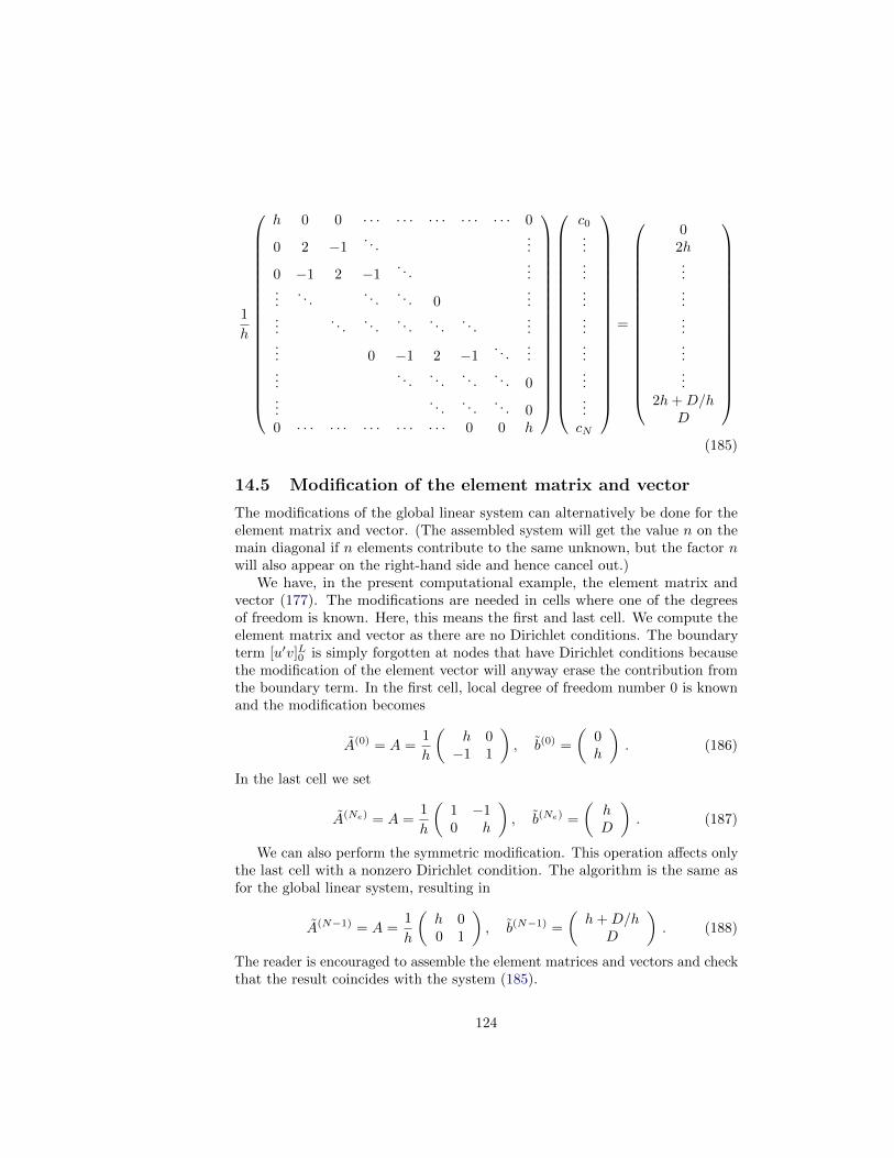
1
h
h 0 0 · · · · · · · · · · · · · · · 0
0 2 −1. . .
...
0 −1 2 −1. . .
......
. . .. . .
. . . 0...
.... . .
. . .. . .
. . .. . .
...... 0 −1 2 −1
. . ....
.... . .
. . .. . .
. . . 0...
. . .. . .
. . . 00 · · · · · · · · · · · · · · · 0 0 h
c0.....................cN
=
02h...............
2h+D/hD
(185)
14.5 Modification of the element matrix and vector
The modifications of the global linear system can alternatively be done for theelement matrix and vector. (The assembled system will get the value n on themain diagonal if n elements contribute to the same unknown, but the factor nwill also appear on the right-hand side and hence cancel out.)
We have, in the present computational example, the element matrix andvector (177). The modifications are needed in cells where one of the degreesof freedom is known. Here, this means the first and last cell. We compute theelement matrix and vector as there are no Dirichlet conditions. The boundaryterm [u′v]L0 is simply forgotten at nodes that have Dirichlet conditions becausethe modification of the element vector will anyway erase the contribution fromthe boundary term. In the first cell, local degree of freedom number 0 is knownand the modification becomes
A(0) = A =1
h
(h 0−1 1
), b(0) =
(0h
). (186)
In the last cell we set
A(Ne) = A =1
h
(1 −10 h
), b(Ne) =
(hD
). (187)
We can also perform the symmetric modification. This operation affects onlythe last cell with a nonzero Dirichlet condition. The algorithm is the same asfor the global linear system, resulting in
A(N−1) = A =1
h
(h 00 1
), b(N−1) =
(h+D/h
D
). (188)
The reader is encouraged to assemble the element matrices and vectors and checkthat the result coincides with the system (185).
124

15 Boundary conditions: specified derivative
Suppose our model problem −u′′(x) = f(x) features the boundary conditionsu′(0) = C and u(L) = D. As already indicated in Section 12, the formercondition can be incorporated through the boundary term that arises fromintegration by parts. This details of this method will now be illustrated in thecontext of finite element basis functions.
15.1 The variational formulation
Starting with the Galerkin method,∫ L
0
(u′′(x) + f(x))ψi(x) dx = 0, i ∈ Is,
integrating u′′ψi by parts results in
∫ L
0
u′(x)′ψ′i(x) dx− (u′(L)ψi(L)− u′(0)ψi(0)) =
∫ L
0
f(x)ψi(x) dx, i ∈ Is .
The first boundary term, u′(L)ψi(L), vanishes because u(L) = D. There aretwo arguments for this result, explained in detail below. The second boundaryterm, u′(0)ψi(0), can be used to implement the condition u′(0) = C, providedψi(0) 6= 0 for some i (but with finite elements we fortunately have ψ0(0) = 1).The variational form of the differential equation then becomes∫ L
0
u′(x)ϕ′i(x) dx+ Cϕi(0) =
∫ L
0
f(x)ϕi(x) dx, i ∈ Is .
15.2 Boundary term vanishes because of the test functions
At points where u is known we may require ψi to vanish. Here, u(L) = D andthen ψi(L) = 0, i ∈ Is. Obviously, the boundary term u′(L)ψi(L) then vanishes.
The set of basis functions ψii∈Is contains in this case all the finite elementbasis functions on the mesh, expect the one that is 1 at x = L. The basisfunction that is left out is used in a boundary function B(x) instead. With aleft-to-right numbering, ψi = ϕi, i = 0, . . . , Nn − 1, and B(x) = DϕNn
:
u(x) = DϕNn(x) +
N=Nn−1∑j=0
cjϕj(x) .
Inserting this expansion for u in the variational form (15.1) leads to the linearsystem
N∑j=0
(∫ L
0
ϕ′i(x)ϕ′j(x) dx
)cj =
∫ L
0
(f(x)ϕi(x)−Dϕ′Nn
(x)ϕi(x))
dx− Cϕi(0),
(189)
125

for i = 0, . . . , N = Nn − 1.
15.3 Boundary term vanishes because of linear systemmodifications
We may, as an alternative to the approach in the previous section, use a basisψii∈Is which contains all the finite element functions on the mesh: ψi = ϕi,i = 0, . . . , Nn = N . In this case, u′(L)ψi(L) = u′(L)ϕi(L) 6= 0 for the icorresponding to the boundary node at x = L (where ϕi = 1). The number ofthis node is i = Nn = N if a left-to-right numbering of nodes is utilized.
However, even though u′(L)ϕN (L) 6= 0, we do not need to compute this term.For i < N we realize that ϕi(L) = 0. The only nonzero contribution to theright-hand side from the affects bN (i = N). Without a boundary function wemust implement the condition u(L) = D by the equivalent statement cN = Dand modify the linear system accordingly. This modification will earse the lastrow and replace bN by another value. Any attempt to compute the boundaryterm u′(L)ϕN (L) and store it in bN will be lost. Therefore, we can safely forgetabout boundary terms corresponding to Dirichlet boundary conditions also whenwe use the methods from Section 14.3 or Section 14.4.
The expansion for u reads
u(x) =∑j∈Is
cjϕj(x), B(x) = DϕN (x),
with N = Nn. Insertion in the variational form (15.1) leads to the linear system
∑j∈Is
(∫ L
0
ϕ′i(x)ϕ′j(x) dx
)cj =
∫ L
0
(f(x)ϕi(x)) dx− Cϕi(0), i ∈ Is . (190)
After having computed the system, we replace the last row by cN = D, eitherstraightforwardly as in Section refreffem:deq:1D:fem:essBC:Bfunc:modsys or in asymmetric fashion as in Section refreffem:deq:1D:fem:essBC:Bfunc:modsys:symm.These modifications can also be performed in the element matrix and vector forthe right-most cell.
15.4 Direct computation of the global linear system
We now turn to actual computations with P1 finite elements. The focus is onhow the linear system and the element matrices and vectors are modified by thecondition u′(0) = C.
Consider first the approach where Dirichlet conditions are incorporated by aB(x) function and the known degree of freedom CNn is left out from the linearsystem (see Section 15.2). The relevant formula for the linear system is givenby (189). There are three differences compared to the extensively computedcase where u(0) = 0 in Sections 13.2 and 13.4. First, because we do not have a
126

Dirichlet condition at the left boundary, we need to extend the linear system (172)with an equation associated with the node x0 = 0. According to Section 14.3, thisextension consists of including A0,0 = 1/h, A0,1 = −1/h, and b0 = h. For i > 0we have Ai,i = 2/h, Ai−1,i = Ai,i+1 = −1/h. Second, we need to include theextra term −Cϕi(0) on the right-hand side. Since all ϕi(0) = 0 for i = 1, . . . , N ,this term reduces to −Cϕ0(0) = −C and affects only the first equation (i = 0).We simply add −C to b0 such that b0 = h − C. Third, the boundary term
−∫ L
0DϕNn
(x)ϕi dx must be computed. Since i = 0, . . . , N = Nn − 1, thisintegral can only get a nonzero contribution with i = Nn − 1 over the last cell.The result becomes −Dh/6. The resulting linear system can be summarized inthe form
1
h
1 −1 0 · · · · · · · · · · · · · · · 0
−1 2 −1. . .
...
0 −1 2 −1. . .
......
. . .. . .
. . . 0...
.... . .
. . .. . .
. . .. . .
...... 0 −1 2 −1
. . ....
.... . .
. . .. . .
. . . 0...
. . .. . .
. . . −10 · · · · · · · · · · · · · · · 0 −1 2
c0.....................cN
=
h− C2h..................
2h−Dh/6
.
(191)
Next we consider the technique where we modify the linear system to incor-porate Dirichlet conditions (see Section 15.3). Now N = Nn. The two differences
from the case above is that the −∫ L
0DϕNnϕi dx term is left out of the right-hand
side and an extra last row associated with the node xNn = L where the Dirichletcondition applies is appended to the system. This last row is anyway replacedby the condition CN = D or this condition can be incorporated in a symmetricfashion. Using the simplest, former approach gives
127

1
h
1 −1 0 · · · · · · · · · · · · · · · 0
−1 2 −1. . .
...
0 −1 2 −1. . .
......
. . .. . .
. . . 0...
.... . .
. . .. . .
. . .. . .
...... 0 −1 2 −1
. . ....
.... . .
. . .. . .
. . . 0...
. . . −1 2 −10 · · · · · · · · · · · · · · · 0 0 1
c0.....................cN
=
h− C2h...............
2hD
.
(192)
15.5 Cellwise computations
Now we compute with one element at a time, working in the reference coordinatesystem X ∈ [−1, 1]. We need to see how the u′(0) = C condition affectsthe element matrix and vector. The extra term −Cϕi(0) in the variationalformulation only affects the element vector in the first cell. On the reference cell,−Cϕi(0) is transformed to −Cϕr(−1), where r counts local degrees of freedom.We have ϕ0(−1) = 1 and ϕ1(−1) = 0 so we are left with the contribution
−Cϕ0(−1) = −C to b(0)0 :
A(0) = A =1
h
(1 1−1 1
), b(0) =
(h− Ch
). (193)
No other element matrices or vectors are affected by the −Cϕi(0) boundaryterm.
There are two alternative ways of incorporating the Dirichlet condition.Following Section 15.2, we get a 1 × 1 element matrix in the last cell and anelement vector with an extra term containing D:
A(e) =1
h
(1), b(e) = h
(1−D/6
), (194)
Alternatively, we include the degree of freedom at the node with u specified.The element matrix and vector must then be modified to constrain the c1 = cNvalue at local node r = 1:
A(Ne) = A =1
h
(1 10 1
), b(Ne) =
(hD
). (195)
128

16 Implementation
It is tempting to create a program with symbolic calculations to perform all thesteps in the computational machinery, both for automating the work and fordocumenting the complete algorithms. As we have seen, there are quite manydetails involved with finite element computations and incorporation of boundaryconditions. An implementation will also act as a structured summary of all thesedetails.
16.1 Global basis functions
We first consider implementations when ψi are global functions are hence differentfrom zero on most of Ω = [0, L] so all integrals need integration over the entiredomain. Since the expressions for the entries in the linear system depend on thedifferential equation problem being solved, the user must supply the necessaryformulas via Python functions. The implementations here attempt to performsymbolic calculations, but fall back on numerical computations if the symbolicones fail.
The user must prepare a function integrand_lhs(psi, i, j) for returningthe integrand of the integral that contributes to matrix entry (i, j). The psi
variable is a Python dictionary holding the basis functions and their derivativesin symbolic form. More precisely, psi[q] is a list of
dqψ0
dxq, . . . ,
dqψNdxq
.
Similarly, integrand_rhs(psi, i) returns the integrand for entry number i inthe right-hand side vector.
Since we also have contributions to the right-hand side vector, and potentiallyalso the matrix, from boundary terms without any integral, we introduce twoadditional functions, boundary_lhs(psi, i, j) and boundary_rhs(psi, i)
for returning terms in the variational formulation that are not to be integratedover the domain Ω. Examples shown later will explain in more detail how theseuser-supplied function may look like.
The linear system can be computed and solved symbolically by the followingfunction:
import sympy as sp
def solve(integrand_lhs, integrand_rhs, psi, Omega,boundary_lhs=None, boundary_rhs=None):
N = len(psi[0]) - 1A = sp.zeros((N+1, N+1))b = sp.zeros((N+1, 1))x = sp.Symbol(’x’)for i in range(N+1):
for j in range(i, N+1):integrand = integrand_lhs(psi, i, j)I = sp.integrate(integrand, (x, Omega[0], Omega[1]))if boundary_lhs is not None:
129

I += boundary_lhs(psi, i, j)A[i,j] = A[j,i] = I # assume symmetry
integrand = integrand_rhs(psi, i)I = sp.integrate(integrand, (x, Omega[0], Omega[1]))if boundary_rhs is not None:
I += boundary_rhs(psi, i)b[i,0] = I
c = A.LUsolve(b)u = sum(c[i,0]*psi[0][i] for i in range(len(psi[0])))return u
Not surprisingly, symbolic solution of differential equations, discretized bya Galerkin or least squares method with global basis functions, is of limitedinterest beyond the simplest problems, because symbolic integration might bevery time consuming or impossible, not only in sympy but also in WolframAlpha(which applies the perhaps most powerful symbolic integration software availabletoday: Mathematica). Numerical integration as an option is therefore desirable.
The extended solve function below tries to combine symbolic and numericalintegration. The latter can be enforced by the user, or it can be invoked after anon-successful symbolic integration (being detected by an Integral object asthe result of the integration in sympy). Note that for a numerical integration,symbolic expressions must be converted to Python functions (using lambdify),and the expressions cannot contain other symbols than x. The real solve routinein the varform1D.py file has error checking and meaningful error messages insuch cases. The solve code below is a condensed version of the real one, withthe purpose of showing how to automate the Galerkin or least squares methodfor solving differential equations in 1D with global basis functions:
def solve(integrand_lhs, integrand_rhs, psi, Omega,boundary_lhs=None, boundary_rhs=None, symbolic=True):
N = len(psi[0]) - 1A = sp.zeros((N+1, N+1))b = sp.zeros((N+1, 1))x = sp.Symbol(’x’)for i in range(N+1):
for j in range(i, N+1):integrand = integrand_lhs(psi, i, j)if symbolic:
I = sp.integrate(integrand, (x, Omega[0], Omega[1]))if isinstance(I, sp.Integral):
symbolic = False # force num.int. hereafterif not symbolic:
integrand = sp.lambdify([x], integrand)I = sp.mpmath.quad(integrand, [Omega[0], Omega[1]])
if boundary_lhs is not None:I += boundary_lhs(psi, i, j)
A[i,j] = A[j,i] = Iintegrand = integrand_rhs(psi, i)if symbolic:
I = sp.integrate(integrand, (x, Omega[0], Omega[1]))if isinstance(I, sp.Integral):
symbolic = Falseif not symbolic:
integrand = sp.lambdify([x], integrand)I = sp.mpmath.quad(integrand, [Omega[0], Omega[1]])
130

if boundary_rhs is not None:I += boundary_rhs(psi, i)
b[i,0] = Ic = A.LUsolve(b)u = sum(c[i,0]*psi[0][i] for i in range(len(psi[0])))return u
16.2 Example: constant right-hand side
To demonstrate the code above, we address
−u′′(x) = b, x ∈ Ω = [0, 1], u(0) = 1, u(1) = 0,
with b as a (symbolic) constant. A possible basis for the space V is ψi(x) =xi+1(1 − x), i ∈ Is. Note that ψi(0) = ψi(1) = 0 as required by the Dirichletconditions. We need a B(x) function to take care of the known boundary valuesof u. Any function B(x) = 1 − xp, p ∈ R, is a candidate, and one arbitrarychoice from this family is B(x) = 1− x3. The unknown function is then writtenas
u(x) = B(x) +∑j∈Is
cjψj(x) .
Let us use the Galerkin method to derive the variational formulation. Multi-plying the differential equation by v and integrate by parts yield∫ 1
0
u′v′ dx =
∫ 1
0
fv dx ∀v ∈ V,
and with u = B +∑j cjψj we get the linear system
∑j∈Is
(∫ 1
0
ψ′iψ′j dx
)cj =
∫ 1
0
(f −B′)ψi dx, i ∈ Is . (196)
The application can be coded as follows in sympy:
x, b = sp.symbols(’x b’)f = bB = 1 - x**3dBdx = sp.diff(B, x)
# Compute basis functions and their derivativesN = 3psi = 0: [x**(i+1)*(1-x) for i in range(N+1)]psi[1] = [sp.diff(psi_i, x) for psi_i in psi[0]]
def integrand_lhs(psi, i, j):return psi[1][i]*psi[1][j]
def integrand_rhs(psi, i):return f*psi[0][i] - dBdx*psi[1][i]
131

Omega = [0, 1]
u_bar = solve(integrand_lhs, integrand_rhs, psi, Omega,verbose=True, symbolic=True)
u = B + u_barprint ’solution u:’, sp.simplify(sp.expand(u))
The printout of u reads -b*x**2/2 + b*x/2 - x + 1. Note that expanding u
and then simplifying is in the present case necessary to get a compact, finalexpression with sympy. A non-expanded u might be preferable in other cases -this depends on the problem in question.
The exact solution ue(x) can be derived by some sympy code that closelyfollows the examples in Section 11.2. The idea is to integrate −u′′ = b twice anddetermine the integration constants from the boundary conditions:
C1, C2 = sp.symbols(’C1 C2’) # integration constantsf1 = sp.integrate(f, x) + C1f2 = sp.integrate(f1, x) + C2# Find C1 and C2 from the boundary conditions u(0)=0, u(1)=1s = sp.solve([u_e.subs(x,0) - 1, u_e.subs(x,1) - 0], [C1, C2])# Form the exact solutionu_e = -f2 + s[C1]*x + s[C2]print ’analytical solution:’, u_eprint ’error:’, sp.simplify(sp.expand(u - u_e))
The last line prints 0, which is not surprising when ue(x) is a parabola and ourapproximate u contains polynomials up to degree 4. It suffices to have N = 1,i.e., polynomials of degree 2, to recover the exact solution.
We can play around with the code and test that with f ∼ xp, the solution isa polynomial of degree p+ 2, and N = p+ 1 guarantees that the approximatesolution is exact.
Although the symbolic code is capable of integrating many choices of f(x),the symbolic expressions for u quickly become lengthy and non-informative,so numerical integration in the code, and hence numerical answers, have thegreatest application potential.
16.3 Finite elements
Implementation of the finite element algorithms for differential equations fol-lows closely the algorithm for approximation of functions. The new additionalingredients are
1. other types of integrands (as implied by the variational formulation)
2. additional boundary terms in the variational formulation for Neumannboundary conditions
3. modification of element matrices and vectors due to Dirichlet boundaryconditions
132

Point 1 and 2 can be taken care of by letting the user supply functions definingthe integrands and boundary terms on the left- and right-hand side of theequation system:
integrand_lhs(phi, r, s, x)boundary_lhs(phi, r, s, x)integrand_rhs(phi, r, x)boundary_rhs(phi, r, x)
Here, phi is a dictionary where phi[q] holds a list of the derivatives of orderq of the basis functions at the an evaluation point; r and s are indices for thecorresponding entries in the element matrix and vector, and x is the globalcoordinate value corresponding to the current evaluation point.
Given a mesh represented by vertices, cells, and dof_map as explained be-fore, we can write a pseudo Python code to list all the steps in the computationalalgorithm for finite element solution of a differential equation.
<Declare global matrix and rhs: A, b>
for e in range(len(cells)):
# Compute element matrix and vectorn = len(dof_map[e]) # no of dofs in this elementh = vertices[cells[e][1]] - vertices[cells[e][1]]<Declare element matrix and vector: A_e, b_e>
# Integrate over the reference cellpoints, weights = <numerical integration rule>for X, w in zip(points, weights):
phi = <basis functions and derivatives at X>detJ = h/2x = <affine mapping from X>for r in range(n):
for s in range(n):A_e[r,s] += integrand_lhs(phi, r, s, x)*detJ*w
b_e[r] += integrand_rhs(phi, r, x)*detJ*w
# Add boundary termsfor r in range(n):
for s in range(n):A_e[r,s] += boundary_lhs(phi, r, s, x)*detJ*w
b_e[r] += boundary_rhs(phi, r, x)*detJ*w
# Incorporate essential boundary conditionsfor r in range(n):
global_dof = dof_map[e][r]if global_dof in essbc_dofs:
# dof r is subject to an essential conditionvalue = essbc_docs[global_dof]# Symmetric modificationb_e -= value*A_e[:,r]A_e[r,:] = 0A_e[:,r] = 0A_e[r,r] = 1b_e[r] = value
# Assemble
133

for r in range(n):for s in range(n):
A[dof_map[e][r], dof_map[e][r]] += A_e[r,s]b[dof_map[e][r] += b_e[r]
<solve linear system>
17 Variational formulations in 2D and 3D
The major difference between deriving variational formulations in 2D and 3Dcompared to 1D is the rule for integrating by parts. A typical second-order termin a PDE may be written in dimension-independent notation as
∇2u or ∇ · (a(x)∇u) .
The explicit forms in a 2D problem become
∇2u = ∇ · ∇u =∂2u
∂x2+∂2u
∂y2,
and
∇ · (a(x)∇u) =∂
∂x
(a(x, y)
∂u
∂x
)+
∂
∂y
(a(x, y)
∂u
∂y
).
We shall continue with the latter operator as the form arises from just settinga = 1.
The general rule for integrating by parts is often referred to as Green’s firstidentity:
−∫
Ω
∇ · (a(x)∇u)v dx =
∫Ω
a(x)∇u · ∇v dx−∫∂Ω
a∂u
∂nv ds, (197)
where ∂Ω is the boundary of Ω and ∂u/∂n = n · ∇u is the derivative of u in theoutward normal direction, n being an outward unit normal to ∂Ω. The integrals∫
Ω() dx are area integrals in 2D and volume integrals in 3D, while
∫∂Ω
() ds is aline integral in 2D and a surface integral in 3D.
Let us divide the boundary into two parts:
• ∂ΩN , where we have Neumann conditions −a ∂u∂n = g, and
• ∂ΩD, where we have Dirichlet conditions u = u0.
The test functions v are required to vanish on ∂ΩD.
134

Example. Here is a quite general, stationary, linear PDE arising in manyproblems:
v · ∇u+ αu = ∇ · (a∇u) + f, x ∈ Ω, (198)
u = u0, x ∈ ∂ΩD, (199)
−a∂u∂n
= g, x ∈ ∂ΩN . (200)
The vector field v and the scalar functions a, α, f , u0, and g may vary with thespatial coordinate x and must be known.
Such a second-order PDE needs exactly one boundary condition at each pointof the boundary, so ∂ΩN ∪ ∂ΩD must be the complete boundary ∂Ω.
Assume that the boundary function u0(x) is defined for all x ∈ Ω. Theunknown function can then be expanded as
u = B +∑j∈Is
cjψj , B = u0 .
The variational formula is obtained from Galerkin’s method, which technicallyimplies multiplying the PDE by a test function v and integrating over Ω:∫
Ω
(v · ∇u+ αu)v dx =
∫Ω
∇ · (a∇u) dx+
∫Ω
fv dx .
The second-order term is integrated by parts, according to∫Ω
∇ · (a∇u) v dx = −∫
Ω
a∇u · ∇v dx+
∫∂Ω
a∂u
∂nv ds .
The variational form now reads
∫Ω
(v · ∇u+ αu)v dx = −∫
Ω
a∇u · ∇v dx+
∫∂Ω
a∂u
∂nv ds+
∫Ω
fv dx .
The boundary term can be developed further by noticing that v 6= 0 only on∂ΩN , ∫
∂Ω
a∂u
∂nv ds =
∫∂ΩN
a∂u
∂nv ds,
and that on ∂ΩN , we have the condition a ∂u∂n = −g, so the term becomes
−∫∂ΩN
gv ds .
The variational form is then
∫Ω
(v · ∇u+ αu)v dx = −∫
Ω
a∇u · ∇v dx−∫∂ΩN
gv ds+
∫Ω
fv dx .
135

Instead of using the integral signs we may use the inner product notation:
(v · ∇u, v) + (αu, v) = −(a∇u,∇v)− (g, v)N + (f, v) .
The subscript N in (g, v)N is a notation for a line or surface integral over ∂ΩN .Inserting the u expansion results in
∑j∈Is
((v · ∇ψj , ψi) + (αψj , ψi) + (a∇ψj ,∇ψi))cj =
(g, ψi)N + (f, ψi)− (v · ∇u0, ψi) + (αu0, ψi) + (a∇u0,∇ψi) .
This is a linear system with matrix entries
Ai,j = (v · ∇ψj , ψi) + (αψj , ψi) + (a∇ψj ,∇ψi)
and right-hand side entries
bi = (g, ψi)N + (f, ψi)− (v · ∇u0, ψi) + (αu0, ψi) + (a∇u0,∇ψi),
for i, j ∈ Is.In the finite element method, we usually express u0 in terms of basis functions
and restrict i and j to run over the degrees of freedom that are not prescribed asDirichlet conditions. However, we can also keep all the cj , j ∈ Is, as unknownsdrop the u0 in the expansion for u, and incorporate all the known cj values inthe linear system. This has been explained in detail in the 1D case.
17.1 Transformation to a reference cell in 2D and 3D
We consider an integral of the type∫Ω(e)
a(x)∇ϕi · ∇ϕj dx, (201)
where the ϕi functions are finite element basis functions in 2D or 3D, defined inthe physical domain. Suppose we want to calculate this integral over a referencecell, denoted by Ωr, in a coordinate system with coordinates X = (X0, X1) (2D)or X = (X0, X1, X2) (3D). The mapping between a point X in the referencecoordinate system and the corresponding point x in the physical coordinatesystem is given by a vector relation x(X). The corresponding Jacobian, J , ofthis mapping has entries
Ji,j =∂xj∂Xi
.
The change of variables requires dx to be replaced by det J dX. The deriva-tives in the ∇ operator in the variational form are with respect to x, whichwe may denote by ∇x. The ϕi(x) functions in the integral are replaced bylocal basis functions ϕr(X) so the integral features ∇xϕr(X). We readily have
136

∇X ϕr(X) from formulas for the basis functions in the reference cell, but thedesired quantity ∇xϕr(X) requires some efforts to compute. All the details areprovided below.
Let i = q(e, r) and consider two space dimensions. By the chain rule,
∂ϕr∂X
=∂ϕi∂X
=∂ϕi∂x
∂x
∂X+∂ϕi∂y
∂y
∂X,
and∂ϕr∂Y
=∂ϕi∂Y
=∂ϕi∂x
∂x
∂Y+∂ϕi∂y
∂y
∂Y.
We can write these two equations as a vector equation[∂ϕr
∂X∂ϕr
∂Y
]=
[∂x∂X
∂y∂X
∂x∂Y
∂y∂Y
] [ ∂ϕi
∂x∂ϕi
∂y
]
Identifying
∇X ϕr =
[∂ϕr
∂X∂ϕr
∂Y
], J =
[∂x∂X
∂y∂X
∂x∂Y
∂y∂Y
], ∇xϕr =
[∂ϕi
∂x∂ϕi
∂y
],
we have the relation
∇X ϕr = J · ∇xϕi,
which we can solve with respect to ∇xϕi:
∇xϕi = J−1 · ∇X ϕr . (202)
On the reference cell, ϕi(x) = ϕr(X), so
∇xϕr(X) = J−1(X) · ∇X ϕr(X) . (203)
This means that we have the following transformation of the integral in thephysical domain to its counterpart over the reference cell:
∫ (e)
Ω
a(x)∇xϕi·∇xϕj dx
∫Ωr
a(x(X))(J−1·∇X ϕr)·(J−1·∇ϕs) detJ dX (204)
17.2 Numerical integration
Integrals are normally computed by numerical integration rules. For multi-dimensional cells, various families of rules exist. All of them are similar towhat is shown in 1D:
∫f dx ≈
∑j wif(xj), where wj are weights and xj are
corresponding points.The file numint.py contains the functions quadrature_for_triangles(n)
and quadrature_for_tetrahedra(n), which returns lists of points and weightscorresponding to integration rules with n points over the reference triangle
137

with vertices (0, 0), (1, 0), (0, 1), and the reference tetrahedron with vertices(0, 0, 0), (1, 0, 0), (0, 1, 0), (0, 0, 1), respectively. For example, the first two rulesfor integration over a triangle have 1 and 3 points:
>>> import numint>>> x, w = numint.quadrature_for_triangles(num_points=1)>>> x[(0.3333333333333333, 0.3333333333333333)]>>> w[0.5]>>> x, w = numint.quadrature_for_triangles(num_points=3)>>> x[(0.16666666666666666, 0.16666666666666666),(0.66666666666666666, 0.16666666666666666),(0.16666666666666666, 0.66666666666666666)]>>> w[0.16666666666666666, 0.16666666666666666, 0.16666666666666666]
Rules with 1, 3, 4, and 7 points over the triangle will exactly integrate polynomialsof degree 1, 2, 3, and 4, respectively. In 3D, rules with 1, 4, 5, and 11 pointsover the tetrahedron will exactly integrate polynomials of degree 1, 2, 3, and 4,respectively.
17.3 Convenient formulas for P1 elements in 2D
We shall now provide some formulas for piecewise linear ϕi functions and theirintegrals in the physical coordinate system. These formulas make it convenient tocompute with P1 elements without the need to work in the reference coordinatesystem and deal with mappings and Jacobians. A lot of computational andalgorithmic details are hidden by this approach.
Let Ω(e) be cell number e, and let the three vertices have global vertexnumbers I, J , and K. The corresponding coordinates are (xI , yI), (xJ , yJ ), and(xK , yK). The basis function ϕI over Ω(e) have the explicit formula
ϕI(x, y) =1
2∆ (αI + βIx+ γIy) , (205)
where
αI = xJyK − xKyJ , (206)
βI = yJ − yK , (207)
γI = xK − xJ , (208)
2∆ = det
1 xI yI1 xJ yJ1 xK yK
. (209)
The quantity ∆ is the area of the cell.The following formula is often convenient when computing element matrices
and vectors:
138
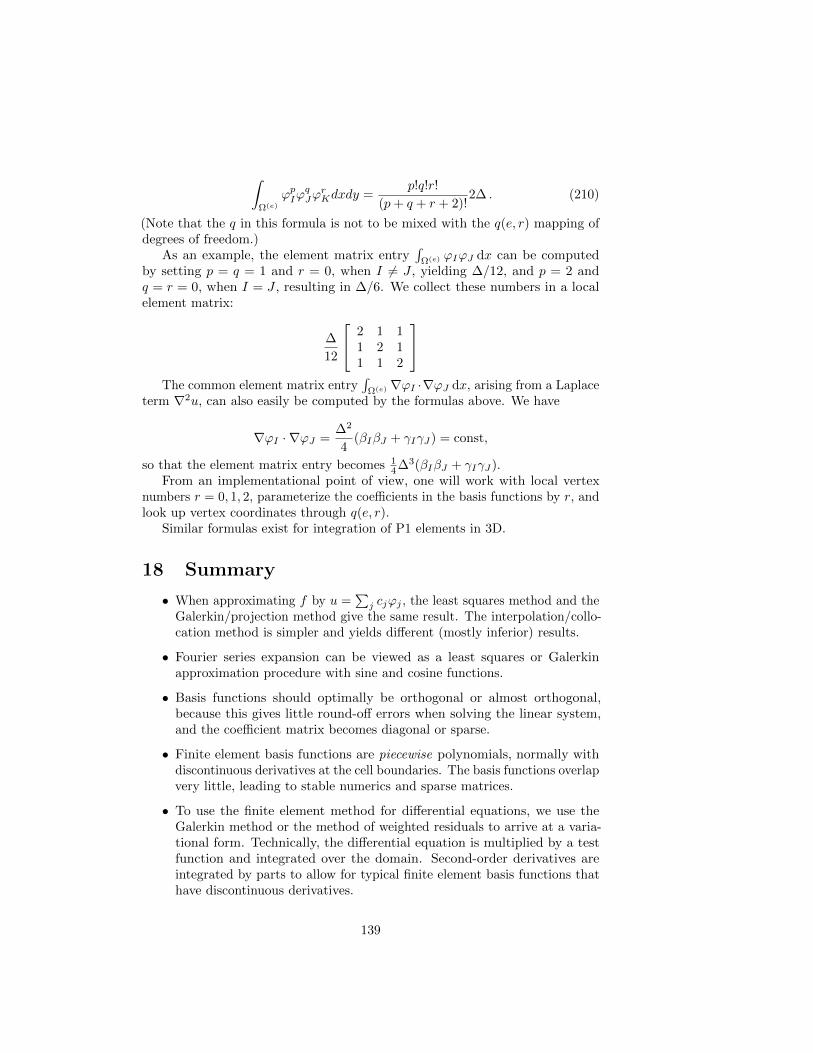
∫Ω(e)
ϕpIϕqJϕ
rKdxdy =
p!q!r!
(p+ q + r + 2)!2∆ . (210)
(Note that the q in this formula is not to be mixed with the q(e, r) mapping ofdegrees of freedom.)
As an example, the element matrix entry∫
Ω(e) ϕIϕJ dx can be computedby setting p = q = 1 and r = 0, when I 6= J , yielding ∆/12, and p = 2 andq = r = 0, when I = J , resulting in ∆/6. We collect these numbers in a localelement matrix:
∆
12
2 1 11 2 11 1 2
The common element matrix entry
∫Ω(e) ∇ϕI ·∇ϕJ dx, arising from a Laplace
term ∇2u, can also easily be computed by the formulas above. We have
∇ϕI · ∇ϕJ =∆2
4(βIβJ + γIγJ) = const,
so that the element matrix entry becomes 14∆3(βIβJ + γIγJ).
From an implementational point of view, one will work with local vertexnumbers r = 0, 1, 2, parameterize the coefficients in the basis functions by r, andlook up vertex coordinates through q(e, r).
Similar formulas exist for integration of P1 elements in 3D.
18 Summary
• When approximating f by u =∑j cjϕj , the least squares method and the
Galerkin/projection method give the same result. The interpolation/collo-cation method is simpler and yields different (mostly inferior) results.
• Fourier series expansion can be viewed as a least squares or Galerkinapproximation procedure with sine and cosine functions.
• Basis functions should optimally be orthogonal or almost orthogonal,because this gives little round-off errors when solving the linear system,and the coefficient matrix becomes diagonal or sparse.
• Finite element basis functions are piecewise polynomials, normally withdiscontinuous derivatives at the cell boundaries. The basis functions overlapvery little, leading to stable numerics and sparse matrices.
• To use the finite element method for differential equations, we use theGalerkin method or the method of weighted residuals to arrive at a varia-tional form. Technically, the differential equation is multiplied by a testfunction and integrated over the domain. Second-order derivatives areintegrated by parts to allow for typical finite element basis functions thathave discontinuous derivatives.
139

• The least squares method is not much used for finite element solution ofdifferential equations of second order, because it then involves second-orderderivatives which cause trouble for basis functions with discontinuousderivatives.
• We have worked with two common finite element terminologies and associ-ated data structures (both are much used, especially the first one, whilethe other is more general):
1. elements, nodes, and mapping between local and global node numbers
2. an extended element concept consisting of cell, vertices, degrees offreedom, local basis functions, geometry mapping, and mapping betweenlocal and global degrees of freedom
• The meaning of the word ”element” is multi-fold: the geometry of a finiteelement (also known as a cell), the geometry and its basis functions, or allinformation listed under point 2 above.
• One normally computes integrals in the finite element method elementby element (cell by cell), either in a local reference coordinate system ordirectly in the physical domain.
• The advantage of working in the reference coordinate system is that themathematical expressions for the basis functions depend on the elementtype only, not the geometry of that element in the physical domain. Thedisadvantage is that a mapping must be used, and derivatives must betransformed from reference to physical coordinates.
• Element contributions to the global linear system are collected in an elementmatrix and vector, which must be assembled into the global system usingthe degree of freedom mapping (dof_map) or the node numbering mapping(elements), depending on which terminology that is used.
• Dirichlet conditions, involving prescribed values of u at the boundary, areimplemented either via a boundary function that take on the right Dirichletvalues, while the basis functions vanish at such boundaries. In the finiteelement method, one has a general expression for the boundary function,but one can also incorporate Dirichlet conditions in the element matrixand vector or in the global matrix system.
• Neumann conditions, involving prescribed values of the derivative (orflux) of u, are incorporated in boundary terms arising from integratingterms with second-order derivatives by part. Forgetting to account for theboundary terms implies the condition ∂u/∂n = 0 at parts of the boundarywhere no Dirichlet condition is set.
140

19 Time-dependent problems
The finite element method is normally used for discretization in space. Thereare two alternative strategies for performing a discretization in time:
• use finite differences for time derivatives to arrive at a recursive set ofspatial problems that can be discretized by the finite element method, or
• discretize in space by finite elements first, and then solve the resultingsystem of ordinary differential equations (ODEs) by some standard methodfor ODEs.
We shall exemplify these strategies using a simple diffusion problem
∂u
∂t= α∇2u+ f(x, t), x ∈ Ω, t ∈ (0, T ], (211)
u(x, 0) = I(x), x ∈ Ω, (212)
∂u
∂n= 0, x ∈ ∂Ω, t ∈ (0, T ] . (213)
Here, u(x, t) is the unknown function, α is a constant, and f(x, t) and I(x)are given functions. We have assigned the particular boundary condition (213)to minimize the details on handling boundary conditions in the finite elementmethod.
19.1 Discretization in time by a Forward Euler scheme
Time discretization. We can apply a finite difference method in time to(211). First we need a mesh in time, here taken as uniform with mesh pointstn = n∆t, n = 0, 1, . . . , Nt. A Forward Euler scheme consists of sampling(211) at tn and approximating the time derivative by a forward difference[D+
t u]n ≈ (un+1 − un)/∆t. This approximation turns (211) into a differentialequation that is discrete in time, but still continuous in space. With a finitedifference operator notation we can write the time-discrete problem as
[D+t u = α∇2u+ f ]n, (214)
for n = 1, 2, . . . , Nt − 1. Writing this equation out in detail and isolating theunknown un+1 on the left-hand side, demonstrates that the time-discrete problemis a recursive set of problems that are continuous in space:
un+1 = un + ∆t(α∇2un + f(x, tn)
). (215)
Given u0 = I, we can use (215) to compute u1, u2, . . . , uNt .For absolute clarity in the various stages of the discretizations, we introduce
ue(x, t) as the exact solution of the space-and time-continuous partial differentialequation (211) and une (x) as the time-discrete approximation, arising from thefinite difference method in time (214). More precisely, ue fulfills
141

∂ue∂t
= α∇2ue + f(x, t), (216)
while un+1e , with a superscript, is the solution of the time-discrete equations
un+1e = une + ∆t
(α∇2une + f(x, tn)
). (217)
Space discretization. We now introduce a finite element approximation toune and un+1
e in (217), where the coefficients depend on the time level:
une ≈ un =
N∑j=0
cnj ψj(x), (218)
un+1e ≈ un+1 =
N∑j=0
cn+1j ψj(x) . (219)
Note that, as before, N denotes the number of degrees of freedom in the spatialdomain. The number of time points is denoted by Nt. We define a space Vspanned by the basis functions ψii∈Is .
19.2 Variational forms
A weighted residual method with weighting functions wi can now be formulated.We insert (218) and (219) in (217) to obtain the residual
R = un+1 − un −∆t(α∇2un + f(x, tn)
).
The weighted residual principle,∫Ω
Rw dx = 0, ∀w ∈W,
results in∫Ω
[un+1 − un −∆t
(α∇2un + f(x, tn)
)]w dx = 0, ∀w ∈W .
From now on we use the Galerkin method so W = V . Isolating the unknownun+1 on the left-hand side gives
∫Ω
un+1ψi dx =
∫Ω
[un −∆t
(α∇2un + f(x, tn)
)]v dx, ∀v ∈ V .
As usual in spatial finite element problems involving second-order derivatives,we apply integration by parts on the term
∫(∇2un)v dx:∫
Ω
α(∇2un)v dx = −∫
Ω
α∇un · ∇v dx+
∫∂Ω
α∂un
∂nv dx .
142

The last term vanishes because we have the Neumann condition ∂un/∂n = 0 forall n. Our discrete problem in space and time then reads
∫Ω
un+1v dx =
∫Ω
unvdx−∆t
∫Ω
α∇un · ∇v dx+ ∆t
∫Ω
fnv dx, ∀v ∈ V .
(220)This is the variational formulation of our recursive set of spatial problems.
Nonzero Dirichlet boundary conditions.
As in stationary problems, we can introduce a boundary function B(x, t)to take care of nonzero Dirichlet conditions:
une ≈ un = B(x, tn) +
N∑j=0
cnj ψj(x), (221)
un+1e ≈ un+1 = B(x, tn+1) +
N∑j=0
cn+1j ψj(x) . (222)
19.3 Simplified notation for the solution at recent timelevels
In a program it is only necessary to store un+1 and un at the same time. Wetherefore drop the n index in programs and work with two functions: u for un+1,the new unknown, and u_1 for un, the solution at the previous time level. Thisis also convenient in the mathematics to maximize the correspondence withthe code. From now on u1 means the discrete unknown at the previous timelevel (un) and u represents the discrete unknown at the new time level (un+1).Equation (220) with this new naming convention is expressed as
∫Ω
uvdx =
∫Ω
u1vdx−∆t
∫Ω
α∇u1 · ∇v dx+ ∆t
∫Ω
fnv dx . (223)
This variational form can alternatively be expressed by the inner product nota-tion:
(u, v) = (u1, v)−∆t(α∇u1,∇v) + (fn, v) . (224)
19.4 Deriving the linear systems
To derive the equations for the new unknown coefficients cn+1j , now just called
cj , we insert
u =
N∑j=0
cjψj(x), u1 =
N∑j=0
c1,jψj(x)
143

in (223) or (224), let the equation hold for all v = ψ, i = 0, . . . ,N, and order theterms as matrix-vector products:
N∑j=0
(ψi, ψj)cj =
N∑j=0
(ψi, ψj)c1,j−∆t
N∑j=0
(∇ψi, α∇ψj)c1,j+(fn, ψi), i = 0, . . . , N .
(225)This is a linear system
∑j Ai,jcj = bi with
Ai,j = (ψi, ψj)
and
bi =
N∑j=0
(ψi, ψj)c1,j −∆t
N∑j=0
(∇ψi, α∇ψj)c1,j + (fn, ψi) .
It is instructive and convenient for implementations to write the linear systemon the form
Mc = Mc1 −∆tKc1 + f, (226)
where
M = Mi,j, Mi,j = (ψi, ψj), i, j ∈ Is,K = Ki,j, Ki,j = (∇ψi, α∇ψj), i, j ∈ Is,f = (f(x, tn), ψi)i∈Is ,c = cii∈Is ,c1 = c1,ii∈Is .
We realize that M is the matrix arising from a term with the zero-th derivativeof u, and called the mass matrix, while K is the matrix arising from a Laplaceterm ∇2u. The K matrix is often known as the stiffness matrix. (The termsmass and stiffness stem from the early days of finite elements when applicationsto vibrating structures dominated. The mass matrix arises from the mass timesacceleration term in Newton’s second law, while the stiffness matrix arises fromthe elastic forces in that law. The mass and stiffness matrix appearing in adiffusion have slightly different mathematical formulas.)
Remark. The mathematical symbol f has two meanings, either the functionf(x, t) in the PDE or the f vector in the linear system to be solved at each timelevel. The symbol u also has different meanings, basically the unknown in thePDE or the finite element function representing the unknown at a time level.The actual meaning should be evident from the context.
144

19.5 Computational algorithm
We observe that M and K can be precomputed so that we can avoid computingthe matrix entries at every time level. Instead, some matrix-vector multiplicationswill produce the linear system to be solved. The computational algorithm hasthe following steps:
1. Compute M and K.
2. Initialize u0 by interpolation or projection
3. For n = 1, 2, . . . , Nt:
(a) compute b = Mc1 −∆tKc1 + f
(b) solve Mc = b
(c) set c1 = c
In case of finite element basis functions, interpolation of the initial conditionat the nodes means c1,j = I(xj). Otherwise one has to solve the linear system∑j ψj(xi)cj = I(xi), where xj denotes an interpolation point. Projection (or
Galerkin’s method) implies solving a linear system with M as coefficient matrix:∑jMi,jc1,j = (I, ψi), i ∈ Is.
19.6 Comparing P1 elements with the finite differencemethod
We can compute the M and K matrices using P1 elements in 1D. A uniformmesh on [0, L] is introduced for this purpose. Since the boundary conditions aresolely of Neumann type in this sample problem, we have no restrictions on thebasis functions ψi and can simply choose ψi = ϕi, i = 0, . . . , N = Nn.
From Section 13.2 or 13.4 we have that the K matrix is the same as we getfrom the finite difference method: h[DxDxu]ni , while from Section 5.2 we knowthat M can be interpreted as the finite difference approximation [u+ 1
6h2DxDxu]ni
(times h). The equation system Mc = b in the algorithm is therefore equivalentto the finite difference scheme
[D+t (u+
1
6h2DxDxu) = αDxDxu+ f ]ni . (227)
(More precisely, Mc = b divided by h gives the equation above.)
Lumping the mass matrix. By applying Trapezoidal integration one canturn M into a diagonal matrix with (h/2, h, . . . , h, h/2) on the diagonal. Thenthere is no need to solve a linear system at each time level, and the finite elementscheme becomes identical to a standard finite difference method
[D+t u = αDxDxu+ f ]ni . (228)
145

The Trapezoidal integration is not as accurate as exact integration andintroduces therefore an error. Whether this error has a good or bad influenceon the overall numerical method is not immediately obvious, and is analyzed indetail in Section 19.10. The effect of the error is at least not more severe thanwhat is produced by the finite difference method.
Making M diagonal is usually referred to as lumping the mass matrix. Thereis an alternative method to using an integration rule based on the node points:one can sum the entries in each row, place the sum on the diagonal, and set allother entries in the row equal to zero. For P1 elements the methods of lumpingthe mass matrix give the same result.
19.7 Discretization in time by a Backward Euler scheme
Time discretization. The Backward Euler scheme in time applied to ourdiffusion problem can be expressed as follows using the finite difference operatornotation:
[D−t u = α∇2u+ f(x, t)]n .
Written out, and collecting the unknown un on the left-hand side and all theknown terms on the right-hand side, the time-discrete differential equationbecomes
une −∆t(α∇2une + f(x, tn)
)= un−1
e . (229)
Equation (229) can compute u1e, u
2e, . . . , u
Nte , if we have a start u0
e = I from theinitial condition. However, (229) is a partial differential equation in space andneeds a solution method based on discretization in space. For this purpose weuse an expansion as in (218)-(219).
Variational forms. Inserting (218)-(219) in (229), multiplying by ψi (orv ∈ V ), and integrating by parts, as we did in the Forward Euler case, results inthe variational form
∫Ω
(unv + ∆tα∇un · ∇v) dx =
∫Ω
un−1v dx−∆t
∫Ω
fnv dx, ∀v ∈ V . (230)
Expressed with u as un and u1 as un−1, this becomes∫Ω
(uv + ∆tα∇u · ∇v) dx =
∫Ω
u1v dx+ ∆t
∫Ω
fnv dx, (231)
or with the more compact inner product notation,
(u, v) + ∆t(α∇u,∇v) = (u1, v) + ∆t(fn, v) . (232)
146

Linear systems. Inserting u =∑j cjψi and u1 =
∑j c1,jψi, and choosing v
to be the basis functions ψi ∈ V , i = 0, . . . , N , together with doing some algebra,lead to the following linear system to be solved at each time level:
(M + ∆tK)c = Mc1 + f, (233)
where M , K, and f are as in the Forward Euler case. This time we really haveto solve a linear system at each time level. The computational algorithm goes asfollows.
1. Compute M , K, and A = M + ∆tK
2. Initialize u0 by interpolation or projection
3. For n = 1, 2, . . . , Nt:
(a) compute b = Mc1 + f
(b) solve Ac = b
(c) set c1 = c
In case of finite element basis functions, interpolation of the initial conditionat the nodes means c1,j = I(xj). Otherwise one has to solve the linear system∑j ψj(xi)cj = I(xi), where xj denotes an interpolation point. Projection (or
Galerkin’s method) implies solving a linear system with M as coefficient matrix:∑jMi,jc1,j = (I, ψi), i ∈ Is.We know what kind of finite difference operators the M and K matrices
correspond to (after dividing by h), so (233) can be interpreted as the followingfinite difference method:
[D−t (u+1
6h2DxDxu) = αDxDxu+ f ]ni . (234)
The mass matrix M can be lumped, as explained in Section 19.6, and thenthe linear system arising from the finite element method with P1 elementscorresponds to a plain Backward Euler finite difference method for the diffusionequation:
[D−t u = αDxDxu+ f ]ni . (235)
19.8 Dirichlet boundary conditions
Suppose now that the boundary condition (213) is replaced by a mixed Neumannand Dirichlet condition,
u(x, t) = u0(x, t), x ∈ ∂ΩD, (236)
−α ∂
∂nu(x, t) = g(x, t), x ∈ ∂ΩN . (237)
147

Using a Forward Euler discretization in time, the variational form at a timelevel becomes
∫Ω
un+1v dx =
∫Ω
(un −∆tα∇un · ∇v) dx−∆t
∫∂ΩN
gv ds, ∀v ∈ V . (238)
Boundary function. The Dirichlet condition u = u0 at ∂ΩD can be incorpo-rated through a boundary function B(x) = u0(x) and demanding that v = 0 at∂ΩD. The expansion for un is written as
un(x) = u0(x, tn) +∑j∈Is
cnj ψj(x) .
Inserting this expansion in the variational formulation and letting it hold for allbasis functions ψi leads to the linear system
∑j∈Is
(∫Ω
ψiψj dx
)cn+1j =
∑j∈Is
(∫Ω
(ψiψj −∆tα∇ψi · ∇ψj) dx
)cnj−∫
Ω
(u0(x, tn+1)− u0(x, tn) + ∆tα∇u0(x, tn) · ∇ψi) dx
+ ∆t
∫Ω
fψi dx−∆t
∫∂ΩN
gψi ds, i ∈ Is .
In the following, we adopt the convention that the unknowns cn+1j are written
as cj , while the known cnj from the previous time level are denoted by c1,j .
Finite element basis functions. When using finite elements, each basisfunction ϕi is associated with a node xi. We have a collection of nodes xii∈Ibon the boundary ∂ΩD. Suppose Unk is the known Dirichlet value at xk at timetn (Unk = u0(xk, tn)). The appropriate boundary function is then
B(x, tn) =∑j∈Ib
Unj ϕj .
The unknown coefficients cj are associated with the rest of the nodes, whichhave numbers ν(i), i ∈ Is = 0, . . . , N. The basis functions for V are chosen asψi = ϕν(i), i ∈ Is, and all of these vanish at the boundary nodes as they should.The expansion for un+1 and un become
un =∑j∈Ib
Unj ϕj +∑j∈Is
c1,jϕν(j),
un+1 =∑j∈Ib
Un+1j ϕj +
∑j∈Is
cjϕν(j) .
148

The equations for the unknown coefficients ci become
∑j∈Is
(∫Ω
ϕiϕj dx
)cj =
∑j∈Is
(∫Ω
(ϕiϕj −∆tα∇ϕi · ∇ϕj) dx
)c1,j−
∑j∈Ib
∫Ω
(ϕiϕj(U
n+1j − Unj ) + ∆tα∇ϕi · ∇ϕjUnj
)dx
+ ∆t
∫Ω
fϕi dx−∆t
∫∂ΩN
gϕi ds, i ∈ Is .
Modification of the linear system. Instead of introducing a boundaryfunction B we can work with basis functions associated with all the nodes andincorporate the Dirichlet conditions by modifying the linear system. Let Is bethe index set that counts all the nodes: 0, 1, . . . , N = Nn. The expansion forun is then
∑j∈Is c
nj ϕj and the variational form becomes
∑j∈Is
(∫Ω
ϕiϕj dx
)cj =
∑j∈Is
(∫Ω
(ϕiϕj −∆tα∇ϕi · ∇ϕj) dx
)c1,j
−∆t
∫Ω
fϕi dx−∆t
∫∂ΩN
gϕi ds .
We introduce the matrices M and K with entries Mi,j =∫
Ωϕiϕj dx and Ki,j =∫
Ωα∇ϕi · ∇ϕj dx, respectively. In addition, we define the vectors c, c1, and f
with entries ci, c1,i, and∫
Ωfϕi dx−
∫∂ΩN
gϕi ds. The equation system can thenbe written as
Mc = Mc1 −∆tKc1 + ∆tf . (239)
When M , K, and b are assembled without paying attention to Dirichlet boundaryconditions, we need to replace equation k by ck = Uk for k correspondingto all boundary nodes (k ∈ Ib). The modification of M consists in settingMk,j = 0, j ∈ Is, and the Mk,k = 1. Alternatively, a modification thatpreserves the symmetry of M can be applied. At each time level one formsb = Mc1 − ∆tKc1 + ∆tf and sets bk = Un+1
k , k ∈ Ib, and solves the systemMc = b.
In case of a Backward Euler method, the system becomes (233). We canwrite the system as Ac = b, with A = M + ∆tK and b = Mc1 + f . Both Mand K needs to be modified because of Dirichlet boundary conditions, but thediagonal entries in K should be set to zero and those in M to unity. In thisway, Ak,k = 1. The right-hand side must read bk = Unk for k ∈ Ib (assuming theunknown is sought at time level tn).
19.9 Example: Oscillating Dirichlet boundary condition
We shall address the one-dimensional initial-boundary value problem
149

ut = (αux)x + f, x ∈ Ω = [0, L], t ∈ (0, T ], (240)
u(x, 0) = 0, x ∈ Ω, (241)
u(0, t) = a sinωt, t ∈ (0, T ], (242)
ux(L, t) = 0, t ∈ (0, T ] . (243)
A physical interpretation may be that u is the temperature deviation froma constant mean temperature in a body Ω that is subject to an oscillatingtemperature (e.g., day and night, or seasonal, variations) at x = 0.
We use a Backward Euler scheme in time and P1 elements of constant lengthh in space. Incorporation of the Dirichlet condition at x = 0 through modifyingthe linear system at each time level means that we carry out the computationsas explained in Section 19.7 and get a system (233). The M and K matricescomputed without paying attention to Dirichlet boundary conditions become
M =h
6
2 1 0 · · · · · · · · · · · · · · · 0
1 4 1. . .
...
0 1 4 1. . .
......
. . .. . .
. . . 0...
.... . .
. . .. . .
. . .. . .
...... 0 1 4 1
. . ....
.... . .
. . .. . .
. . . 0...
. . . 1 4 10 · · · · · · · · · · · · · · · 0 1 2
(244)
K =α
h
1 −1 0 · · · · · · · · · · · · · · · 0
−1 2 −1. . .
...
0 −1 2 −1. . .
......
. . .. . .
. . . 0...
.... . .
. . .. . .
. . .. . .
...... 0 −1 2 −1
. . ....
.... . .
. . .. . .
. . . 0...
. . . −1 2 −10 · · · · · · · · · · · · · · · 0 −1 1
(245)
The right-hand side of the variational form contains Mc1 since there is no sourceterm (f) and no boundary term from the integration by parts (ux = 0 at x = L
150

and we compute as if ux = 0 at x = 0 too). We must incorporate the Dirichletboundary condition c0 = a sinωtn by ensuring that this is the first equation inthe linear system. To this end, the first row in K and M are set to zero, butthe diagonal entry M0,0 is set to 1. The right-hand side is b = Mc1, and we setb0 = a sinωtn. Note that in this approach, N = Nn, and c equals the unknownu at each node in the mesh. We can write the complete linear system as
c0 = a sinωtn, (246)
h
6(ci−1 + 4ci + ci+1) + ∆t
α
h(−ci−1 + 2ci + ci+1) =
h
6(c1,i−1 + 4c1,i + c1,i+1),
(247)
i = 1, . . . , Nn − 1,
h
6(ci−1 + 2ci) + ∆t
α
h(−ci−1 + ci) =
h
6(c1,i−1 + 2c1,i), i = Nn .
(248)
The Dirichlet boundary condition can alternatively be implemented througha boundary function B(x, t) = a sinωtϕ0(x):
un(x) = a sinωtnϕ0(x) +∑j∈Is
cjϕν(j)(x), ν(j) = j + 1 .
Now, N = Nn − 1 and the c vector contains values of u at nodes 1, 2, . . . , Nn.The right-hand side gets a contribution
∫ L
0
(a(sinωtn − sinωtn−1)ϕ0ϕi −∆tαa sinωtn∇ϕ0 · ∇ϕi) dx . (249)
19.10 Analysis of the discrete equations
The diffusion equation ut = αuxx allows a (Fourier) wave component u =exp (βt+ ikx) as solution if β = −αk2, which follows from inserting the wavecomponent in the equation. The exact wave component can alternatively bewritten as
u = Ane eikx, Ae = e−αk
2∆t . (250)
Many numerical schemes for the diffusion equation has a similar wave componentas solution:
unq = Aneikx, (251)
where is an amplification factor to be calculated by inserting (252) in the scheme.We introduce x = qh, or x = q∆x to align the notation with that frequentlyused in finite difference methods.
151

A convenient start of the calculations is to establish some results for variousfinite difference operators acting on
unq = Aneikq∆x . (252)
[D+t A
neikq∆x]n = Aneikq∆xA− 1
∆t,
[D−t Aneikq∆x]n = Aneikq∆x
1−A−1
∆t,
[DtAneikq∆x]n+ 1
2 = An+ 12 eikq∆x
A12 −A− 1
2
∆t= Aneikq∆x
A− 1
∆t,
[DxDxAneikq∆x]q = −An 4
∆x2sin2
(k∆x
2
).
Forward Euler discretization. We insert (252) in the Forward Euler schemewith P1 elements in space and f = 0 (this type of analysis can only be carriedout if f = 0),
[D+t (u+
1
6h2DxDxu) = αDxDxu]nq . (253)
We have
[D+t DxDxAe
ikx]nq = [D+t A]n[DxDxe
ikx]q = −Aneikp∆xA− 1
∆t
4
∆x2sin2(
k∆x
2) .
The term [D+t Ae
ikx + 16∆x2D+
t DxDxAeikx]nq then reduces to
A− 1
∆t− 1
6∆x2A− 1
∆t
4
∆x2sin2(
k∆x
2),
orA− 1
∆t
(1− 2
3sin2(k∆x/2)
).
Introducing p = k∆x/2 and C = α∆t/∆x2, the complete scheme becomes
(A− 1)
(1− 2
3sin2 p
)= −4C sin2 p,
from which we find A to be
A = 1− 4Csin2 p
1− 23 sin2 p
.
How does this A change the stability criterion compared to the ForwardEuler finite difference scheme and centered differences in space? The stabilitycriterion is |A| ≤ 1, which here implies A ≤ 1 and A ≥ −1. The former is alwaysfulfilled, while the latter leads to
152
4Csin2 p
1 + 23 sin2 p
≤ 2 .
The factor sin2 p/(1− 23 sin2 p) can be plotted for p ∈ [0, π/2], and the maximum
value goes to 3 as p→ π/2. The worst case for stability therefore occurs for theshortest possible wave, p = π/2, and the stability criterion becomes
C ≤ 1
6⇒ ∆t ≤ ∆x2
6α, (254)
which is a factor 1/3 worse than for the standard Forward Euler finite differencemethod for the diffusion equation, which demands C ≤ 1/2. Lumping the massmatrix will, however, recover the finite difference method and therefore implyC ≤ 1/2 for stability.
Backward Euler discretization. We can use the same approach and insert(252) in the Backward Euler scheme with P1 elements in space and f = 0:
[D−t (u+1
6h2DxDxu) = αDxDxu]ni . (255)
Similar calculations as in the Forward Euler case lead to
(1−A−1)
(1− 2
3sin2 p
)= −4C sin2 p,
and hence
A =
(1 + 4C
sin2 p
1− 23 sin2 p
)−1
.
Comparing amplification factors. It is of interest to compare A and Ae asfunctions of p for some C values. Figure 48 display the amplification factorsfor the Backward Euler scheme corresponding a coarse mesh with C = 2 and amesh at the stability limit of the Forward Euler scheme in the finite differencemethod, C = 1/2. Figures 49 and 50 shows how the accuracy increases withlower C values for both the Forward Euler and Backward schemes, respectively.The striking fact, however, is that the accuracy of the finite element methodis significantly less than the finite difference method for the same value of C.Lumping the mass matrix to recover the numerical amplification factor A of thefinite difference method is therefore a good idea in this problem.
Remaining tasks:
• Taylor expansion of the error in the amplification factor Ae −A
• Taylor expansion of the error e = (Ane −An)eikx
• L2 norm of e
153

0.0 0.2 0.4 0.6 0.8 1.0 1.2 1.4 1.60.0
0.2
0.4
0.6
0.8
1.0 Method: BE
C=2, FEMC=2, FDMC=1/2, FEMC=1/2, FDMexact
Figure 48: Comparison of coarse-mesh amplification factors for Backward Eulerdiscretization of a 1D diffusion equation.
0.0 0.2 0.4 0.6 0.8 1.0 1.2 1.4 1.61.0
0.5
0.0
0.5
1.0 Method: FE
C=1/6, FEMC=1/6, FDMC=1/12, FEMC=1/12, FDMexact
Figure 49: Comparison of fine-mesh amplification factors for Forward Eulerdiscretization of a 1D diffusion equation.
154

0.0 0.2 0.4 0.6 0.8 1.0 1.2 1.4 1.60.3
0.4
0.5
0.6
0.7
0.8
0.9
1.0 Method: BE
C=1/6, FEMC=1/6, FDMC=1/12, FEMC=1/12, FDMexact
Figure 50: Comparison of fine-mesh amplification factors for Backward Eulerdiscretization of a 1D diffusion equation.
155

20 Systems of differential equations
Many mathematical models involve m + 1 unknown functions governed by asystem of m + 1 differential equations. In abstract form we may denote theunknowns by u(0), . . . , u(m) and write the governing equations as
L0(u(0), . . . , u(m)) = 0,
...
Lm(u(0), . . . , u(m)) = 0,
where Li is some differential operator defining differential equation number i.
20.1 Variational forms
There are basically two ways of formulating a variational form for a system ofdifferential equations. The first method treats each equation independently asa scalar equation, while the other method views the total system as a vectorequation with a vector function as unknown.
Let us start with the one equation at a time approach. We multiply equationnumber i by some test function v(i) ∈ V (i) and integrate over the domain:
∫Ω
L(0)(u(0), . . . , u(m))v(0) dx = 0, (256)
... (257)∫Ω
L(m)(u(0), . . . , u(m))v(m) dx = 0 . (258)
Terms with second-order derivatives may be integrated by parts, with Neumannconditions inserted in boundary integrals. Let
V (i) = spanψ(i)0 , . . . , ψ
(i)Ni,
such that
u(i) = B(i)(x) +
Ni∑j=0
c(i)j ψ
(i)j (x),
where B(i) is a boundary function to handle nonzero Dirichlet conditions. Observethat different unknowns live in different spaces with different basis functions andnumbers of degrees of freedom.
From the m equations in the variational forms we can derive m coupled
systems of algebraic equations for the Πmi=0Ni unknown coefficients c
(i)j , j =
0, . . . , Ni, i = 0, . . . ,m.
156

The alternative method for deriving a variational form for a system ofdifferential equations introduces a vector of unknown functions
u = (u(0), . . . , u(m)),
a vector of test functions
v = (u(0), . . . , u(m)),
with
u,v ∈ V = V (0) × · · · × V (m) .
With nonzero Dirichlet conditions, we have a vector B = (B(0), . . . , B(m)) withboundary functions and then it is u−B that lies in V , not u itself.
The governing system of differential equations is written
L(u) = 0,
where
L(u) = (L(0)(u), . . . ,L(m)(u)) .
The variational form is derived by taking the inner product of the vector ofequations and the test function vector:∫
Ω
L(u) · v = 0 ∀v ∈ V . (259)
Observe that (259) is one scalar equation. To derive systems of algebraicequations for the unknown coefficients in the expansions of the unknown func-tions, one chooses m linearly independent v vectors to generate m independentvariational forms from (259). The particular choice v = (v(0), 0, . . . , 0) recovers(256), v = (0, . . . , 0, v(m) recovers (258), and v = (0, . . . , 0, v(i), 0, . . . , 0) recoversthe variational form number i,
∫ΩL(i)v(i) dx = 0, in (256)-(258).
20.2 A worked example
We now consider a specific system of two partial differential equations in twospace dimensions:
µ∇2w = −β, (260)
κ∇2T = −µ||∇w||2 . (261)
The unknown functions w(x, y) and T (x, y) are defined in a domain Ω, whileµ, β, and κ are given constants. The norm in (261) is the standard Euclediannorm:
||∇w||2 = ∇w · ∇w = w2x + w2
y .
157

The boundary conditions associated with (260)-(261) are w = 0 on ∂Ω andT = T0 on ∂Ω. Each of the equations (260) and (261) need one condition ateach point on the boundary.
The system (260)-(261) arises from fluid flow in a straight pipe, with the z axisin the direction of the pipe. The domain Ω is a cross section of the pipe, w is thevelocity in the z direction, µ is the viscosity of the fluid, β is the pressure gradientalong the pipe, T is the temperature, and κ is the heat conduction coefficientof the fluid. The equation (260) comes from the Navier-Stokes equations, and(261) follows from the energy equation. The term −µ||∇w||2 models heating ofthe fluid due to internal friction.
Observe that the system (260)-(261) has only a one-way coupling: T dependson w, but w does not depend on T , because we can solve (260) with respectto w and then (261) with respect to T . Some may argue that this is not areal system of PDEs, but just two scalar PDEs. Nevertheless, the one-waycoupling is convenient when comparing different variational forms and differentimplementations.
20.3 Identical function spaces for the unknowns
Let us first apply the same function space V for w and T (or more precisely,w ∈ V and T − T0 ∈ V ). With
V = spanψ0(x, y), . . . , ψN (x, y),
we write
w =
N∑j=0
c(w)j ψj , T = T0 +
N∑j=0
c(T )j ψj . (262)
Note that w and T in (260)-(261) denote the exact solution of the PDEs, whilew and T (262) are the discrete functions that approximate the exact solution.It should be clear from the context whether a symbol means the exact orapproximate solution, but when we need both at the same time, we use asubscript e to denote the exact solution.
Variational form of each individual PDE. Inserting the expansions (262)in the governing PDEs, results in a residual in each equation,
Rw = µ∇2w + β, (263)
RT = κ∇2T + µ||∇w||2 . (264)
A Galerkin method demands Rw and RT do be orthogonal to V :
158

∫Ω
Rwv dx = 0 ∀v ∈ V,∫Ω
RT v dx = 0 ∀v ∈ V .
Because of the Dirichlet conditions, v = 0 on ∂Ω. We integrate the Laplaceterms by parts and note that the boundary terms vanish since v = 0 on ∂Ω:
∫Ω
µ∇w · ∇v dx =
∫Ω
βv dx ∀v ∈ V, (265)∫Ω
κ∇T · ∇v dx =
∫Ω
µ∇w · ∇w v dx ∀v ∈ V . (266)
Compound scalar variational form. The alternative way of deriving thevariational from is to introduce a test vector function v ∈ V = V × V and takethe inner product of v and the residuals, integrated over the domain:∫
Ω
(Rw, RT ) · v dx = 0 ∀v ∈ V .
With v = (v0, v1) we get∫Ω
(Rwv0 +RT v1) dx = 0 ∀v ∈ V .
Integrating the Laplace terms by parts results in
∫Ω
(µ∇w ·∇v0 +κ∇T ·∇v1) dx =
∫Ω
(βv0 +µ∇w ·∇w v1) dx, ∀v ∈ V . (267)
Choosing v0 = v and v1 = 0 gives the variational form (265), while v0 = 0 andv1 = v gives (266).
With the inner product notation, (p, q) =∫
Ωpq dx, we can alternatively write
(265) and (266) as
(µ∇w,∇v) = (β, v) ∀v ∈ V,(κ∇T,∇v) = (µ∇w · ∇w, v) ∀v ∈ V,
or since µ and κ are considered constant,
µ(∇w,∇v) = (β, v) ∀v ∈ V, (268)
κ(∇T,∇v) = µ(∇w · ∇w, v) ∀v ∈ V . (269)
159

Decoupled linear systems. The linear systems governing the coefficients
c(w)j and c
(T )j , j = 0, . . . , N , are derived by inserting the expansions (262) in
(265) and (266), and choosing v = ψi for i = 0, . . . , N . The result becomes
N∑j=0
A(w)i,j c
(w)j = b
(w)i , i = 0, . . . , N, (270)
N∑j=0
A(T )i,j c
(T )j = b
(T )i , i = 0, . . . , N, (271)
A(w)i,j = µ(∇ψj ,∇ψi), (272)
b(w)i = (β, ψi), (273)
A(T )i,j = κ(∇ψj ,∇ψi), (274)
b(T )i = µ((
∑j
c(w)j ∇ψj) · (
∑k
c(w)k ∇ψk), ψi) . (275)
It can also be instructive to write the linear systems using matrices andvectors. Define K as the matrix corresponding to the Laplace operator ∇2. Thatis, Ki,j = (∇ψj ,∇ψi). Let us introduce the vectors
b(w) = (b(w)0 , . . . , b
(w)N ),
b(T ) = (b(T )0 , . . . , b
(T )N ),
c(w) = (c(w)0 , . . . , c
(w)N ),
c(T ) = (c(T )0 , . . . , c
(T )N ) .
The system (270)-(271) can now be expressed in matrix-vector form as
µKc(w) = b(w), (276)
κKc(T ) = b(T ) . (277)
We can solve the first system for c(w), and then the right-hand side b(T ) isknown such that we can solve the second system for c(T ).
Coupled linear systems. Despite the fact that w can be computed first,without knowing T , we shall now pretend that w and T enter a two-way couplingsuch that we need to derive the algebraic equations as one system for all the
unknowns c(w)j and c
(T )j , j = 0, . . . , N . This system is nonlinear in c
(w)j because
of the ∇w · ∇w product. To remove this nonlinearity, imagine that we introducean iteration method where we replace ∇w · ∇w by ∇w− · ∇w, w− being the wcomputed in the previous iteration. Then the term ∇w− · ∇w is linear in wsince w− is known. The total linear system becomes
160

N∑j=0
A(w,w)i,j c
(w)j +
N∑j=0
A(w,T )i,j c
(T )j = b
(w)i , i = 0, . . . , N, (278)
N∑j=0
A(T,w)i,j c
(w)j +
N∑j=0
A(T,T )i,j c
(T )j = b
(T )i , i = 0, . . . , N, (279)
A(w,w)i,j = µ(∇ψj , ψi), (280)
A(w,T )i,j = 0, (281)
b(w)i = (β, ψi), (282)
A(w,T )i,j = µ((∇ψw−) · ∇ψj), ψi), (283)
A(T,T )i,j = κ(∇ψj , ψi), (284)
b(T )i = 0 . (285)
This system can alternatively be written in matrix-vector form as
µKc(w) = 0b(w), (286)
Lc(w) + κKc(T ) = 0, (287)
with L as the matrix from the ∇w− · ∇ operator: Li,j = A(w,T )i,j .
The matrix-vector equations are often conveniently written in block form:(µK 0L κK
)(c(w)
c(T )
)=
(b(w)
0
),
Note that in the general case where all unknowns enter all equations, wehave to solve the compound system (297)-(298) since then we cannot utilize thespecial property that (270) does not involve T and can be solved first.
When the viscosity depends on the temperature, the µ∇2w term must bereplaced by ∇ · (µ(T )∇w), and then T enters the equation for w. Now we havea two-way coupling since both equations contain w and T and therefore mustbe solved simultaneously Th equation ∇ · (µ(T )∇w) = −β is nonlinear, and ifsome iteration procedure is invoked, where we use a previously computed T− inthe viscosity (µ(T−)), the coefficient is known, and the equation involves onlyone unknown, w. In that case we are back to the one-way coupled set of PDEs.
We may also formulate our PDE system as a vector equation. To this end, weintroduce the vector of unknowns u = (u(0), u(1)), where u(0) = w and u(1) = T .We then have
∇2u =
(−µ−1β
−κ−1µ∇u(0) · ∇u(0)
).
161

20.4 Different function spaces for the unknowns
It is easy to generalize the previous formulation to the case where w ∈ V (w) andT ∈ V (T ), where V (w) and V (T ) can be different spaces with different numbersof degrees of freedom. For example, we may use quadratic basis functions forw and linear for T . Approximation of the unknowns by different finite elementspaces is known as mixed finite element methods.
We write
V (w) = spanψ(w)0 , . . . , ψ
(w)Nw,
V (T ) = spanψ(T )0 , . . . , ψ
(T )NT .
The next step is to multiply (260) by a test function v(w) ∈ V (w) and (261) by av(T ) ∈ V (T ), integrate by parts and arrive at
∫Ω
µ∇w · ∇v(w) dx =
∫Ω
βv(w) dx ∀v(w) ∈ V (w), (288)∫Ω
κ∇T · ∇v(T ) dx =
∫Ω
µ∇w · ∇w v(T ) dx ∀v(T ) ∈ V (T ) . (289)
The compound scalar variational formulation applies a test vector functionv = (v(w), v(T )) and reads
∫Ω
(µ∇w · ∇v(w) + κ∇T · ∇v(T )) dx =
∫Ω
(βv(w) + µ∇w · ∇w v(T )) dx, (290)
valid ∀v ∈ V = V (w) × V (T ).The associated linear system is similar to (270)-(271) or (297)-(298), except
that we need to distinguish between ψ(w)i and ψ
(T )i , and the range in the sums
over j must match the number of degrees of freedom in the spaces V (w) andV (T ). The formulas become
Nw∑j=0
A(w)i,j c
(w)j = b
(w)i , i = 0, . . . , Nw, (291)
NT∑j=0
A(T )i,j c
(T )j = b
(T )i , i = 0, . . . , NT , (292)
A(w)i,j = µ(∇ψ(w)
j , ψ(w)i ), (293)
b(w)i = (β, ψ
(w)i ), (294)
A(T )i,j = κ(∇ψ(T )
j , ψ(T )i ), (295)
b(T )i = µ(∇w−, ψ(T )
i ) . (296)
162

In the case we formulate one compound linear system involving both c(w)j ,
j = 0, . . . , Nw, and c(T )j , j = 0, . . . , NT , (297)-(298) becomes
Nw∑j=0
A(w,w)i,j c
(w)j +
NT∑j=0
A(w,T )i,j c
(T )j = b
(w)i , i = 0, . . . , Nw, (297)
Nw∑j=0
A(T,w)i,j c
(w)j +
NT∑j=0
A(T,T )i,j c
(T )j = b
(T )i , i = 0, . . . , NT , (298)
A(w,w)i,j = µ(∇ψ(w)
j , ψ(w)i ), (299)
A(w,T )i,j = 0, (300)
b(w)i = (β, ψ
(w)i ), (301)
A(w,T )i,j = µ(∇w− · ∇ψ(w)
j ), ψ(T )i ), (302)
A(T,T )i,j = κ(∇ψ(T )
j , ψ(T )i ), (303)
b(T )i = 0 . (304)
The corresponding block form(µK(w) 0L κK(T )
)(c(w)
c(T )
)=
(b(w)
0
),
has square and rectangular block matrices: K(w) is Nw ×Nw, K(T ) is NT ×NT ,while L is NT ×Nw,
20.5 Computations in 1D
We can reduce the system (260)-(261) to one space dimension, which correspondsto flow in a channel between two flat plates. Alternatively, one may considerflow in a circular pipe, introduce cylindrical coordinates, and utilize the radialsymmetry to reduce the equations to a one-dimensional problem in the radialcoordinate. The former model becomes
µwxx = −β, (305)
κTxx = −µw2x, (306)
while the model in the radial coordinate r reads
µ1
r
d
dr
(rdw
dr
)= −β, (307)
κ1
r
d
dr
(rdT
dr
)= −µ
(dw
dr
)2
. (308)
163

The domain for (305)-(306) is Ω = [0, H], with boundary conditions w(0) =w(H) = 0 and T (0) = T (H) = T0. For (307)-(308) the domain is [0, R] (R beingthe radius of the pipe) and the boundary conditions are du/dr = dT/dr = 0 forr = 0, u(R) = 0, and T (R) = T0.
Calculations to be continued...
21 Exercises
Exercise 23: Refactor functions into a more general class
Section 11.2 displays three functions for computing the analytical solution ofsome simple model problems. There is quite some repetitive code, suggestingthat the functions can benefit from being refactored into a class where the usercan define the f(x), a(x), and the boundary conditions in particular methodsin subclasses. Demonstrate how the new class can be used to solve the threeparticular problems in Section 11.2.
In the method that computes the solution, check that the solution found fulfillsthe differential equation and the boundary conditions. Filename: uxx_f_sympy_class.py.
Exercise 24: Compute the deflection of a cable with sinefunctions
A hanging cable of length L with significant tension has a downward deflectionw(x) governed by
Solve
Tw′′(x) = `(x),
where T is the tension in the cable and `(x) the load per unit length. The cableis fixed at x = 0 and x = L so the boundary conditions become T (0) = T (L) = 0.We assume a constant load `(x) = const.
The solution is expected to be symmetric around x = L/2. Formulating theproblem for x ∈ Ω = [0, L/2] and then scaling it, results in the scaled problemfor the dimensionless vertical deflection u:
u′′ = 1, x ∈ (0, 1), u(0) = 0, u′(1) = 0 .
Introduce the function space spanned by ψi = sin((i + 1)πx/2), i = 1, . . . , N .Use a Galerkin and a least squares method to find the coefficients cj in u(x) =∑j cjψj . Find how fast the coefficients decrease in magnitude by looking at
cj/cj−1. Find the error in the maximum deflection at x = 1 when only one basisfunction is used (N = 0).
What happens if we choose basis functions ψi = sin((i+ 1)πx)? These basisfunctions are appropriate if we do not utilize symmetry and solve the problemon [0, L]. A scaled version of this problem reads
u′′ = 1, x ∈ (0, 1), u(0) = u(1) = 0 .
164

Carry out the computations with N = 0 and demonstrate that the maximumdeflection u(1/2) is the same in the problem utilizing symmetry and the problemcovering the whole cable. Filename: cable_sin.pdf.
Exercise 25: Check integration by parts
Consider the Galerkin method for the problem involving u in Exercise 24. Showthat the formulas for cj are independent of whether we perform integration byparts or not. Filename: cable_integr_by_parts.pdf.
Exercise 26: Compute the deflection of a cable with 2 P1elements
Solve the problem for u in Exercise 24 using two P1 linear elements. Filename:cable_2P1.pdf.
Exercise 27: Compute the deflection of a cable with 1 P2element
Solve the problem for u in Exercise 24 using one P2 element with quadratic basisfunctions. Filename: cable_1P2.pdf.
Exercise 28: Compute the deflection of a cable with a stepload
We consider the deflection of a tension cable as described in Exercise 24. Nowthe load is
`(x) =
`1, x < L/2,`2, x ≥ L/2 x ∈ [0, L] .
This load is not symmetric with respect to the midpoint x = L/2 so the solutionloses its symmetry and we must solve the scaled problem
u′′ =
1, x < 1/2,0, x ≥ 1/2
x ∈ (0, 1), u(0) = 0, u(1) = 0 .
a) Use ψi = sin((i + 1)πx), i = 0, . . . , N and the Galerkin method withoutintegration by parts. Derive a formula for cj in the solution expansion u =∑j cjψj . Plot how fast the coefficients cj tend to zero (on a log scale).
b) Solve the problem with P1 finite elements. Plot the solution for Ne = 2, 4, 8elements.
Filename: cable_discont_load.pdf.
165

Exercise 29: Show equivalence between linear systems
Incorporation of Dirichlet conditions at x = 0 and x = L in a finite elementmesh on Ω = [0, L] can either be done by introducing an expansion u(x) =
U0ϕ0 + UNnϕNn
+∑Nj=0 cjϕν(j), with N = Nn − 2 and considering u values
at the inner nodes as unknowns, or one can assemble the matrix system withu(x) =
∑N=Nn
j=0 cjϕj and afterwards replace the rows corresponding to known cjvalues by the boundary conditions. Show that the two approaches are equivalent.
Exercise 30: Compute with a non-uniform mesh
Derive the linear system for the problem −u′′ = 2 on [0, 1], with u(0) = 0and u(1) = 1, using P1 elements and a non-uniform mesh. The vertices havecoordinates x0 = 0 < x1 < · · · < xN = 1, and the length of cell number e ishe = xe+1 − xe.
It is of interest to compare the discrete equations for the finite elementmethod in a non-uniform mesh with the corresponding discrete equations arisingfrom a finite difference method. Go through the derivation of the finite differenceformula u′′(xi) ≈ [DxDxu]i and modify it to find a natural discretization ofu′′(xi) on a non-uniform mesh. Filename: nonuniform_P1.pdf.
Problem 31: Solve a 1D finite element problem by hand
The following scaled 1D problem is a very simple, yet relevant, model forconvective transport in fluids:
u′ = εu′′, u(0) = 0, u(1) = 1, x ∈ [0, 1] . (309)
a) Find the analytical solution to this problem. (Introduce w = u′, solve thefirst-order differential equation for w(x), and integrate once more.)
b) Derive the variational form of this problem.
c) Introduce a finite element mesh with uniform partitioning. Use P1 elementsand compute the element matrix and vector for a general element.
d) Incorporate the boundary conditions and assemble the element contribu-tions.
e) Identify the resulting linear system as a finite difference discretization ofthe differential equation using
[D2xu = εDxDxu]i .
166

f) Compute the numerical solution and plot it together with the exact solutionfor a mesh with 20 elements and ε = 10, 1, 0.1, 0.01.
Filename: convdiff1D_P1.pdf.
Exercise 32: Compare finite elements and differences for aradially symmetric Poisson equation
We consider the Poisson problem in a disk with radius R with Dirichlet conditionsat the boundary. Given that the solution is radially symmetric and hencedependent only on the radial coordinate (r =
√x2 + y2), we can reduce the
problem to a 1D Poisson equation
− 1
r
d
dr
(rdu
dr
)= f(r), r ∈ (0, R), u′(0) = 0, u(R) = UR . (310)
a) Derive a variational form of (310) by integrating over the whole disk, orposed equivalently: use a weighting function 2πrv(r) and integrate r from 0 toR.
b) Use a uniform mesh partition with P1 elements and show what the resultingset of equations becomes. Integrate the matrix entries exact by hand, but use aTrapezoidal rule to integrate the f term.
c) Explain that an intuitive finite difference method applied to (310) gives
1
ri
1
h2
(ri+ 1
2(ui+1 − ui)− ri− 1
2(ui − ui−1)
)= fi, i = rh .
For i = 0 the factor 1/ri seemingly becomes problematic. One must alwayshave u′(0) = 0, because of the radial symmetry, which implies u−1 = u1, if weallow introduction of a fictitious value u−1. Using this u−1 in the differenceequation for i = 0 gives
1
r0
1
h2
(r 1
2(u1 − u0)− r− 1
2(u0 − u1)
)=
1
r0
1
2h2((r0 + r1)(u1 − u0)− (r−1 + r0)(u0 − u1)) ≈ 2(u1 − u0),
if we use r−1 + r1 ≈ 2r0.
Set up the complete set of equations for the finite difference method andcompare to the finite element method in case a Trapezoidal rule is used tointegrate the f term in the latter method.
Filename: radial_Poisson1D_P1.pdf.
167

Exercise 33: Compute with variable coefficients and P1 el-ements by hand
Consider the problem
− d
dx
(a(x)
du
dx
)+ γu = f(x), x ∈ Ω = [0, L], u(0) = α, u′(L) = β . (311)
We choose a(x) = 1 + x2. Then
u(x) = α+ β(1 + L2) tan−1(x), (312)
is an exact solution if f(x) = γu.
Derive a variational formulation and compute general expressions for theelement matrix and vector in an arbitrary element, using P1 elements and auniform partitioning of [0, L]. The right-hand side integral is challenging andcan be computed by a numerical integration rule. The Trapezoidal rule (101)gives particularly simple expressions. Filename: atan1D_P1.pdf.
Exercise 34: Solve a 2D Poisson equation using polynomialsand sines
The classical problem of applying a torque to the ends of a rod can be modeledby a Poisson equation defined in the cross section Ω:
−∇2u = 2, (x, y) ∈ Ω,
with u = 0 on ∂Ω. Exactly the same problem arises for the deflection of amembrane with shape Ω under a constant load.
For a circular cross section one can readily find an analytical solution. For arectangular cross section the analytical approach ends up with a sine series. Theidea in this exercise is to use a single basis function to obtain an approximateanswer.
We assume for simplicity that the cross section is the unit square: Ω =[0, 1]× [0, 1].
a) We consider the basis ψp,q(x, y) = sin((p + 1)πx) sin(qπy), p, q = 0, . . . , n.These basis functions fulfill the Dirichlet condition. Use a Galerkin method andn = 0.
b) The basis function involving sine functions are orthogonal. Use thisproperty in the Galerkin method to derive the coefficients cp,q in a formulau =
∑p
∑q cp,qψp,q(x, y).
168

c) Another possible basis is ψi(x, y) = (x(1−x)y(1− y))i+1, i = 0, . . . , N . Usethe Galerkin method to compute the solution for N = 0. Which choice of asingle basis function is best, u ∼ x(1 − x)y(1 − y) or u ∼ sin(πx) sin(πy)? Inorder to answer the question, it is necessary to search the web or the literaturefor an accurate estimate of the maximum u value at x = y = 1/2.
Filename: torsion_sin_xy.pdf.
Exercise 35: Analyze a Crank-Nicolson scheme for the dif-fusion equation
Perform the analysis in Section 19.10 for a 1D diffusion equation ut = αuxxdiscretized by the Crank-Nicolson scheme in time:
un+1 − un
∆t= α
1
2
(un+1
∂x2
un
∂x2
),
or written compactly with finite difference operators,
[Dtu = αDxDxut]n+ 1
2 .
(From a strict mathematical point of view, the un and un+1 in these equationsshould be replaced by une and un+1
e to indicate that the unknown is the exactsolution of the PDE discretized in time, but not yet in space, see Section 19.1.)Make plots similar to those in Section 19.10. Filename: fe_diffusion.pdf.
169

Index
affine mapping, 47, 81approximation
by sines, 20collocation, 24interpolation, 25of functions, 13of general vectors, 11of vectors in the plane, 7
assembly, 45
cell, 64cells list, 65chapeau function, 40Chebyshev nodes, 29collocation method (approximation), 24
degree of freedom, 64dof map, 64dof map list, 65
edges, 79element matrix, 44essential boundary condition, 107
faces, 79finite element basis function, 40finite element expansion
reference element, 65finite element mesh, 33finite element, definition, 64
Galerkin methodfunctions, 15vectors, 10, 12
Gauss-Legendre quadrature, 70
hat function, 40Hermite polynomials, 68
integration by parts, 100interpolation, 25isoparametric mapping, 82
Kronecker delta, 27, 36
Lagrange (interpolating) polynomial,26
least squreas methodvectors, 9
linear elements, 40lumped mass matrix, 63, 146
mapping of reference cellsaffine mapping, 47isoparametric mapping, 82
mass lumping, 63, 146mass matrix, 63, 144, 146mesh
finite elements, 33Midpoint rule, 69mixed finite elements, 162
natural boundary condition, 107Newton-Cotes rules, 69numerical integration
Midpoint rule, 69Newton-Cotes formulas, 69Simpson’s rule, 69Trapezoidal rule, 69
P1 element, 40P2 element, 40projection
functions, 15vectors, 10, 12
quadratic elements, 40
reference cell, 64residual, 93Runge’s phenomenon, 28
simplex elements, 79simplices, 79Simpson’s rule, 69sparse matrices, 58stiffness matrix, 144strong form, 101
170

tensor product, 71test function, 95test space, 95Trapezoidal rule, 69trial function, 95trial space, 95
variational formulation, 95vertex, 64vertices list, 65
weak form, 101
171