Embed Size (px)
Citation preview
Introduction to Multisim SchematicCapture and SPICE Simulation
By:Erik Luther
Janell Rodriguez

Introduction to Multisim SchematicCapture and SPICE Simulation
By:Erik Luther
Janell Rodriguez
Online:< http://cnx.org/content/col10369/1.3/ >
C O N N E X I O N S
Rice University, Houston, Texas

This selection and arrangement of content as a collection is copyrighted by Erik Luther, Janell Rodriguez. It is
licensed under the Creative Commons Attribution 2.0 license (http://creativecommons.org/licenses/by/2.0/).
Collection structure revised: September 26, 2006
PDF generated: October 26, 2012
For copyright and attribution information for the modules contained in this collection, see p. 81.

Table of Contents
1 Introduction
1.1 Objectives for the National Instruments Multisim Course . . . . . . . . . . . . . . . . . . . . . . . . . . . . . . . . . . . . 11.2 Interactive Schematic Capture and Layout in National Instruments Multisim . . . . . . . . . . . . . . . . 41.3 Exercise: Introducing the National Instruments Multisim Environment . . . . . . . . . . . . . . . . . . . . . . . 9
2 Schematic Capture
2.1 Electrical and Electronic Components Available in National Instruments Multisim . . . . . . . . . . . . . 112.2 Exercise: Finding and Placing Components in National Instruments Multisim . . . . . . . . . . . . . . . 192.3 Electrical and Electronic Component Manipulation in National Instruments Mul-
tisim . . . . . . . . . . . . . . . . . . . . . . . . . . . . . . . . . . . . . . . . . . . . . . . . . . . . . . . . . . . . . . . . . . . . . . . . . . . . . . . . . . . . . . . 212.4 Exercise: Drawing A Schematic in National Instruments Multisim . . . . . . . . . . . . . . . . . . . . . . . . . . 26
3 Circuits
3.1 Creating Circuits in Multisim . . . . . . . . . . . . . . . . . . . . . . . . . . . . . . . . . . . . . . . . . . . . . . . . . .. . . . . . . . . . . . . 293.2 Using Electrical Rules Checking in National Instruments Multisim . . . . . . . . . . . . . . . . . . . . . . . . . . 313.3 Creating and Using Sub-Circuits in National Instruments Multisim . . . . . . . . . . . . . . . . . . . . . . . . . 333.4 Generating Schematic Reports and Annotation in National Instruments Multisim . . . . . . . . . . . . . 36
4 Simulation
4.1 Simulating Circuits using the SPICE in National Instruments Multisim . . . . . . . . . . . . . . . . . . . . . 394.2 Instrumenting a Circuit Simulation in National Instruments Multisim . . . . . . . . . . . . . . . . . . . . . . . 444.3 Exercise: Instrumenting Simulated Circuits in National Instruments Multisim . . . . . . . . . . . . . . . 504.4 Creating LabVIEW Instruments to Instrument Circuit Simulations in National
Instruments Multisim . . . . . . . . . . . . . . . . . . . . . . . . . . . . . . . . . . . . . . . . . . . . . . . . . . . . . . . . . . . . . . . . . . . . . . . 534.5 Analyses of Circuit Simulations . . . . . . . . . . . . . . . . . . . . . . . . . . . . . . . . . . . . . . . . . . . . . . . . . . . . . . . . . . . . . 564.6 Exercise: Analysis of Circuit Simulations in National Instruments Multisim . . . . . . . . . . . . . . . . . 62
5 Integrated Design and Academic Features
5.1 Integrated Design with Multisim and Other National Instruments Products . . . . . . . . . . . . . . . . . 695.2 Enhanced Educational Features for Teaching with National Instruments Multisim . . . . . . . . . . . . . 74
Attributions . . . . . . . . . . . . . . . . . . . . . . . . . . . . . . . . . . . . . . . . . . . . . . . . . . . . . . . . . . . . . . . . . . . . . . . . . . . . . . . . . . . . . . . . . 81

iv
Available for free at Connexions <http://cnx.org/content/col10369/1.3>
Chapter 1
Introduction
1.1 Objectives for the National Instruments Multisim Course1
1.1.1 Introduction
1.1.1.1 Course Objectives and Overview
This course will provide you with an introduction to Multisim's many features. At the end of the threehours, you should have a basic understanding of the user interface (UI), schematic capture and simulation.You will also see how Multisim ts into the broader PCB design ow (Figure 1 and Figure 2).
The course is split into sections, each containing associated exercises to help solidify the concepts pre-sented. There is also an Appendix, which provides some direction on how to integrate Multisim with NationalInstruments' products to create a truly integrated benchtop platform for design and verication.
1.1.1.2 Course Materials
In order to successfully complete this course, you will need the following:
• Multisim Software.• Multisim User Guide and helples (available in soft copies installed with the software).• Associated circuits (associated circuits found on the CD in the back of this book).
1This content is available online at <http://cnx.org/content/m13746/1.1/>.
Available for free at Connexions <http://cnx.org/content/col10369/1.3>
1

2 CHAPTER 1. INTRODUCTION
1.1.1.3 The Electronics Workbench Portfolio
Figure 1.1: Electronics Workbench Product Flow
1.1.1.3.1 Multicap
Multicap 9 is the industry's most intuitive and powerful schematic capture program. Multicap's innovativeand timesaving features, including modeless operation, powerful autowiring and a comprehensive databaseorganized into logical parts bins on your desktop, allow designs to be captured almost as fast as they can beconceptualized. Repetitive tasks are optimized, leaving you freer to create, test and ultimately perfect yourdesigns, resulting in superior products and minimizing time-to-market.
1.1.1.3.2 Multisim
Multisim, the world's only interactive circuit simulator, allows you to design better products in less time.Multisim includes a completely integrated version of Multicap, making it the ideal tool for capturing schemat-ics and then instantly simulating circuits.
Multisim 9 also oers integration with National Instruments LabVIEW and SignalExpress, allowing youto tightly integrate design and test.
1.1.1.3.3 Ultiboard
Ultiboard has been carefully designed to maximize your productivity. By optimizing the most commonrepetitive tasks such as part and trace placement, the number of keystrokes and mouse movements requiredto lay out any design has been dramatically reduced.
Ultiboard handles today's higher speed designs with ease using constraint driven layout. Innovativefeatures such as Real-Time design rule checking, Push & Shove components & traces, component nudgingwith trace rubberbanding, Follow-me trace editing and an Automatic Connection machine ensure that yourapidly complete an error-free board.
1.1.1.3.4 Ultiroute for Professional Customers
For all but the most basic PCBs, the density and complexity of today's designs make manual componentand trace placement techniques impractical. For these designs, Electronics Workbench oers Ultiroute astate-of-the-art autorouting and autoplacement tool.
Ultiroute ensures high circuit performance and lower production costs for these demanding projects byuniquely combining the best of gridless (shape-based) and grid-based routing.
Available for free at Connexions <http://cnx.org/content/col10369/1.3>

3
1.1.1.4 Integrated Design and Validation with National Instruments
Figure 1.2: The Integrated Design Flow
Available for free at Connexions <http://cnx.org/content/col10369/1.3>

4 CHAPTER 1. INTRODUCTION
1.1.1.4.1 LabVIEW
NI LabVIEW is the graphical development environment for creating exible and scalable test, measurement,and control applications rapidly and at minimal cost. With LabVIEW, engineers and scientists interface withreal-world signals, analyze data for meaningful information, and share results and applications. Regardlessof experience, LabVIEW makes development fast and easy for all users.
1.1.1.4.2 SignalExpress
SignalExpress is interactive software for quickly acquiring, comparing, automating, and storing measure-ments. Use SignalExpress to streamline your exploratory and automated measurement tasks for electronicsdesign, validation, and test.
SignalExpress introduces an innovative approach to conguring your measurements using intuitive drag-and-drop steps that do not require code development.
1.1.1.4.3 NI ELVIS
National Instruments Educational Laboratory Virtual Instrumentation Suite (NI ELVIS) is a LabVIEW-based design and prototyping environment for university science and engineering laboratories. NI ELVISconsists of LabVIEW-based virtual instruments, a multifunction data acquisition device, and a custom-designed benchtop workstation and prototyping board. This combination provides a ready-to-use suite ofinstruments found in all educational laboratories. Because it is based on LabVIEW and provides completedata acquisition and prototyping capabilities, the system is ideal for academic coursework, from lower-division classes to advanced project-based curricula. Curriculum applications include electronics design,communications, controls, mechatronics, instrumentation, and data acquisition.
1.2 Interactive Schematic Capture and Layout in National Instru-
ments Multisim2
1.2.1 Schematic Capture in MultiSim
1.2.1.1 The Benets of Integrated Capture and Simulation
Multisim provides users with the unique ability to capture and simulate from within the very same integratedenvironment. The advantages of this approach are many. Users new to Multisim do not have to worry aboutsophisticated SPICE (Simulation Program with Integrated Circuit Emphasis) syntax and commands, whileadvanced users have easy access to all SPICE details.
Multisim makes capturing schematics easier and more intuitive than ever. A spreadsheet view allowsusers to easily modify characteristics of any number of components simultaneously: from PBC footprint toSPICE model. Modeless operation provides the most ecient way of placing components and wiring themtogether. Working with both analog and digital multisection components is intuitive and simple.
In addition to traditional SPICE analyses, Multisim allows users to intuitively connect virtual instrumentsto their schematics. Virtual instruments make it fast and easy to view interactive simulation results byreplicating the real-world environment.
Multisim also provides special components known as interactive parts which can be modied while asimulation is running. Interactive parts such as switches and potentiometers, will immediately and accuratelyaect the results of simulation.
When the need arises for more advanced analysis, Multisim delivers over 15 sophisticated analyses. Someexamples of analyses include AC, Monte Carlo, Worst Case, and Fourier. Provided natively within theMultisim environment is a powerful Grapher, which allows the customized viewing of simulation data andanalyses.
2This content is available online at <http://cnx.org/content/m13745/1.1/>.
Available for free at Connexions <http://cnx.org/content/col10369/1.3>

5
The integrated capture and simulation environment provided by Multisim is a natural t for any circuitdesigner, and will save both time and frustration throughout the entire circuit design process.
1.2.1.2 The Multisim Environment
1.2.1.2.1 Introducing the Multisim Environment
Multisim's user interface consists of the basic elements, illustrated in Figure 1 below.
Figure 1.3: The MultiSim Environment
Available for free at Connexions <http://cnx.org/content/col10369/1.3>

6 CHAPTER 1. INTRODUCTION
1.2.1.2.2 The Design Toolbox
The Design Toolbox is used to manage various elements in the schematic. The Visibility tab lets you choosewhich layers to display on the current sheet on the workspace. The Hierarchy tab contains a tree that showsthe dependencies of the les in the design that you have open. The Project tab displays information aboutthe current project. Users can add les to the existing folders of the current project, control access to les,and archive designs.
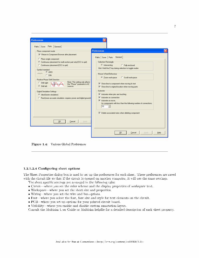
1.2.1.2.3 Conguring global options
Global options allow users to congure specics of the Multisim environment. They can be modied byaccessing the preferences dialog box. Choose Options/Global Preferences. The Preferences dialog boxappears, oering you the following tabs:• Pathswhere you can change the lepaths for the databases and other settings.• Savewhere you set up Auto-backup timing and whether you want to save simulation data with
instruments.• Partswhere you set up component placement mode and the symbol standard (ANSI or DIN). You
also set up default digital simulation settings.• Generalwhere you set up selection rectangle behavior, mouse wheel behavior, bus wiring and auto-
wiring behavior.
Available for free at Connexions <http://cnx.org/content/col10369/1.3>
7
Figure 1.4: Various Global Preferences
1.2.1.2.4 Conguring sheet options
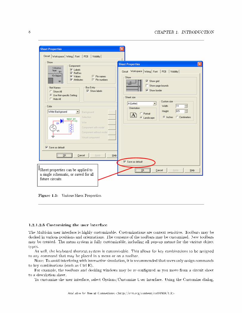
The Sheet Properties dialog box is used to set up the preferences for each sheet. These preferences are savedwith the circuit le so that if the circuit is opened on another computer, it will use the same settings.
The sheet specic settings are arranged in the following tabs:• Circuitwhere you set the color scheme and the display properties of workspace text.• Workspacewhere you set the sheet size and properties.• Wiringwhere you set the wire and bus options.• Fontwhere you select the font, font size and style for text elements on the circuit.• PCBwhere you set up options for your printed circuit board.• Visibilitywhere you enable and disable custom annotation layers.Consult the Multisim User Guide or Multisim helple for a detailed description of each sheet property.
Available for free at Connexions <http://cnx.org/content/col10369/1.3>
8 CHAPTER 1. INTRODUCTION
Figure 1.5: Various Sheet Properties
1.2.1.2.5 Customizing the user interface
The Multisim user interface is highly customizable. Customizations are context sensitive. Toolbars may bedocked in various positions and orientations. The contents of the toolbars may be customized. New toolbarsmay be created. The menu system is fully customizable, including all pop-up menus for the various objecttypes.
As well, the keyboard shortcut system is customizable. This allows for key combinations to be assignedto any command that may be placed in a menu or on a toolbar.
Note: To avoid interfering with interactive simulation, it is recommended that users only assign commandsto key combinations (such as Ctrl-E).
For example, the toolbars and docking windows may be re-congured as you move from a circuit sheetto a description sheet.
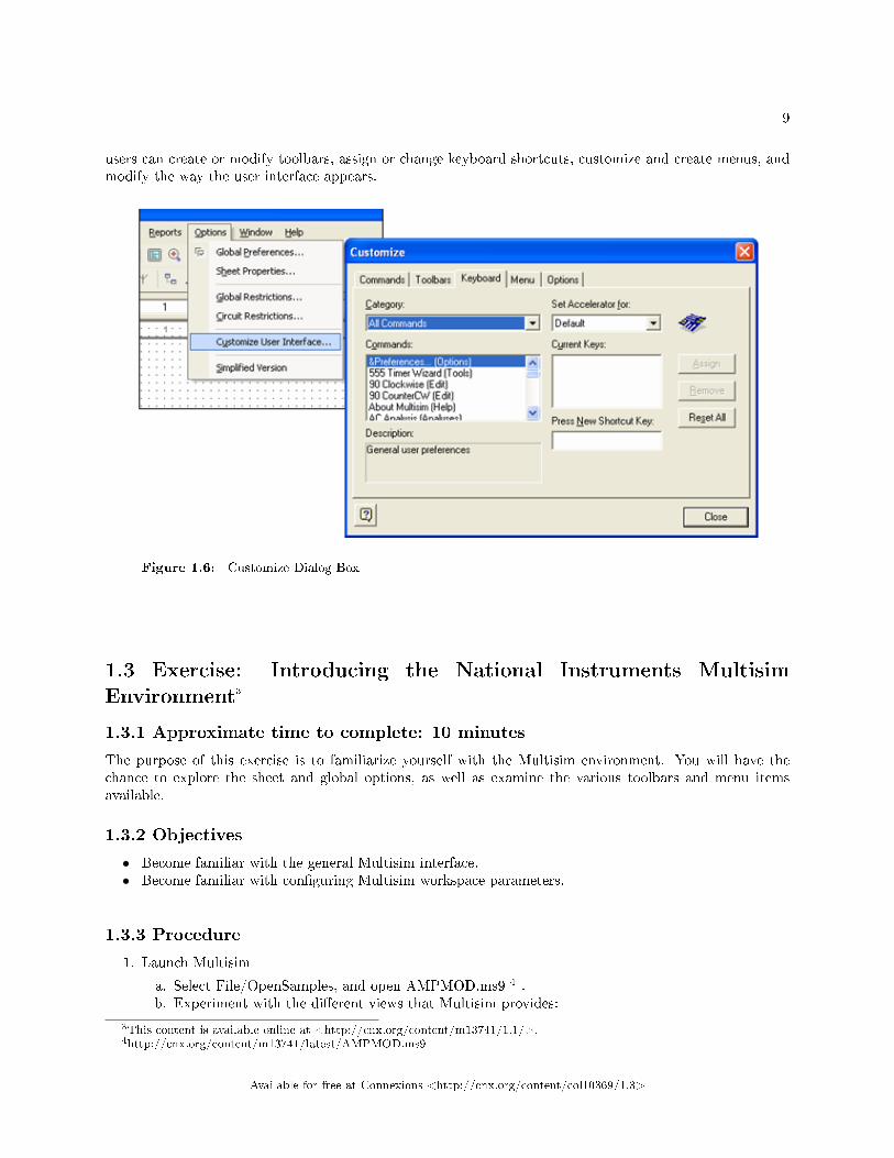
To customize the user interface, select Options/Customize User Interface. Using the Customize dialog,
Available for free at Connexions <http://cnx.org/content/col10369/1.3>
9
users can create or modify toolbars, assign or change keyboard shortcuts, customize and create menus, andmodify the way the user interface appears.
Figure 1.6: Customize Dialog Box
1.3 Exercise: Introducing the National Instruments Multisim
Environment3
1.3.1 Approximate time to complete: 10 minutes
The purpose of this exercise is to familiarize yourself with the Multisim environment. You will have thechance to explore the sheet and global options, as well as examine the various toolbars and menu itemsavailable.
1.3.2 Objectives
• Become familiar with the general Multisim interface.• Become familiar with conguring Multisim workspace parameters.
1.3.3 Procedure
1. Launch Multisim
a. Select File/OpenSamples, and open AMPMOD.ms9 4 .b. Experiment with the dierent views that Multisim provides:
3This content is available online at <http://cnx.org/content/m13741/1.1/>.4http://cnx.org/content/m13741/latest/AMPMOD.ms9
Available for free at Connexions <http://cnx.org/content/col10369/1.3>

10 CHAPTER 1. INTRODUCTION
1. Select View/Spreadsheet to toggle the spreadsheet view.2. Browse the Nets, Components,and PCB Layerstabs.3. How many uniquely numbered nets are there?__________
c. Select View/Circuit Description Box.This is where designers can view detailed information abouttheir design. To edit the contents, select Tools/Description Box Editor.
d. Select View/Design Toolbox.This view gives designers insight into the les, sub-circuits and otherelements of a given design.
2. Experiment with Global Preferences and Sheet Properties.
a. Select Options/Sheet Properties.
1. Try toggling on and o the grid in the Workspace tab (to view the changes, click OK orApply).
2. Try switching the colors of the environment in the Circuittab (to view the changes, click OKor Apply).
b. Select Options/Global Preferences.
1. Enable the Auto-backup feature in the Save tab.2. Toggle on or o the Return to Component Browser check box in the Parts tab according to
your personal preference.
3. Examine the settings under the Generaltab. What is the default Selection Rectangle mode?4. If time permits, continuing experimenting with the Multisim environment. Try to place an arbitrary
component onto the schematic.5. Close the schematic by clicking File/Close.
End of Exercise
AMPMOD.ms95
5http://cnx.org/content/m13741/latest/AMPMOD.ms9
Available for free at Connexions <http://cnx.org/content/col10369/1.3>

Chapter 2
Schematic Capture
2.1 Electrical and Electronic Components Available in National In-
struments Multisim1
2.1.1 Components
2.1.1.1 Components Overview
Components comprise the basis for any schematic. A component is any part that can be placed onto theschematic. Multisim denes two broad categories of parts: real and virtual. It is important to understandthe dierence between these parts, in order to fully utilize their advantages.
Real components can be dierentiated from virtual parts because real components have a specic valuethat cannot be changed, and a PCB footprint.
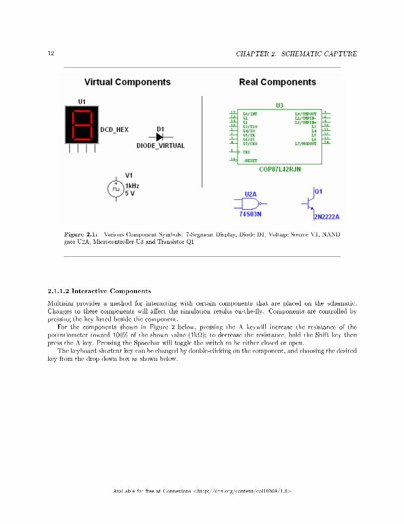
Virtual components are simulation-only components, which can be assigned user-dened characteristics.For example, a virtual resistor can take on any resistance (such as 3.86654 Ohms). Virtual components helpdesigners to check calculations by simulating designs with precise component values. Virtual componentscan also be idealized components such as the 4-pin Hex display shown in Figure 1.
Multisim also provides other classications of components: analog, digital, mixed-mode, animated, in-teractive, multi-section digital, electromechanical, and radio-frequency (RF) components.
1This content is available online at <http://cnx.org/content/m13735/1.1/>.
Available for free at Connexions <http://cnx.org/content/col10369/1.3>
11
12 CHAPTER 2. SCHEMATIC CAPTURE
Figure 2.1: Various Component Symbols: 7-Segment Display, Diode D1, Voltage Source V1, NANDgate U2A, Microcontroller U3 and Transistor Q1
2.1.1.2 Interactive Components
Multisim provides a method for interacting with certain components that are placed on the schematic.Changes to these components will aect the simulation results on-the-y. Components are controlled bypressing the key listed beside the component.
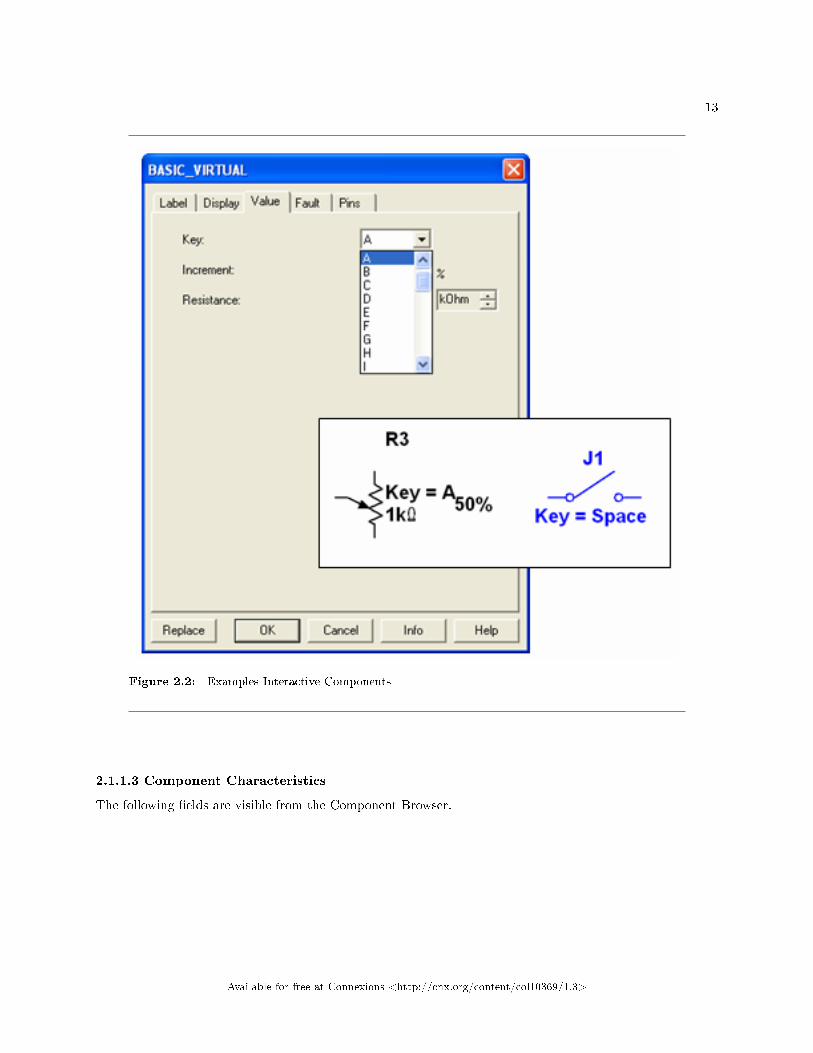
For the components shown in Figure 2 below, pressing the A keywill increase the resistance of thepotentiometer toward 100% of the shown value (1kΩ); to decrease the resistance, hold the Shift key thenpress the A key. Pressing the Spacebar will toggle the switch to be either closed or open.
The keyboard shortcut key can be changed by double-clicking on the component, and choosing the desiredkey from the drop-down box as shown below.
Available for free at Connexions <http://cnx.org/content/col10369/1.3>
13
Figure 2.2: Examples Interactive Components
2.1.1.3 Component Characteristics
The following elds are visible from the Component Browser.
Available for free at Connexions <http://cnx.org/content/col10369/1.3>

14 CHAPTER 2. SCHEMATIC CAPTURE
Figure 2.3: Component Information
2.1.1.4 The Component Browser
The Component Browser is used to select components for placement onto the schematic. To access theComponent Browser, click on any icon in the parts bin, or select Place/Component. The default keyboardshortcut to place a component is Ctrl-W.Double-click on the desired component to place it on the schematic.The component will ghost the mouse cursor until the left mouse button is clicked again to place thecomponent.
Available for free at Connexions <http://cnx.org/content/col10369/1.3>
15
Figure 2.4: The Parts Bin or Component Toolbar
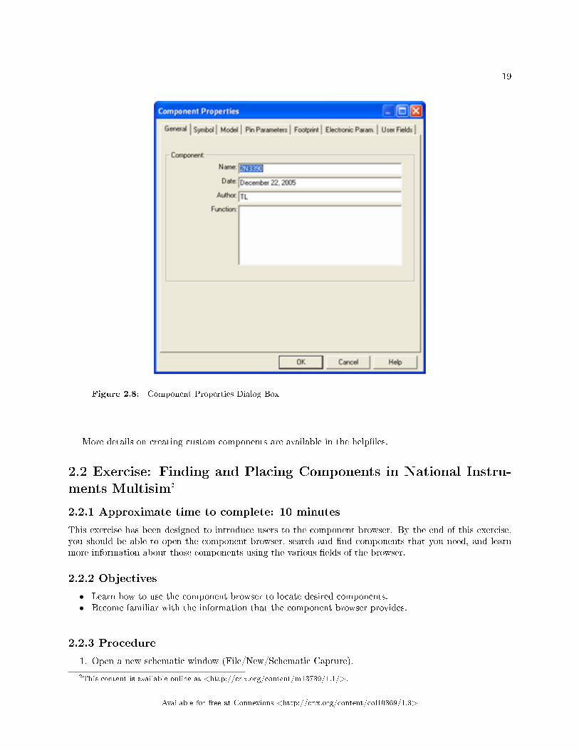
Figure 2.5: The Component Browser
Available for free at Connexions <http://cnx.org/content/col10369/1.3>

16 CHAPTER 2. SCHEMATIC CAPTURE
To search this view, simply start typing the name of the desired component, and the browser will au-tomatically display matching candidate parts. Optionally, for a more detailed search, click on the Searchbutton.
The Component Browser shows the current database in which the displayed parts are stored. Multisimorganizes the parts by group, and family. The browser also shows the symbol, a description of the componentin the Function eld, the model, and the footprint / manufacturer.
The wildcard character `*'can be used to match any set of characters. For example LM*78 would matchcomponents LM*AD would return both LM101AD and LM108AD, among others.
Note:Any component may have multiple models associated with it. Each model may account for varyingphysical characteristics of the component. For example, the LM358M opamp has ve visible pins, but onlythree of them are used in one model, ignoring the power supply terminals. More information about modelscan be found by selecting the desired model from the Model Manuf.\ID eld, and click on the Model button.
2.1.1.5 Databases
There are three levels of database provided by Multisim:
• The Master Database is read-only, and contains components supplied by Electronics Workbench.• The User Database is private to the individual user logged onto the computer. It is used for components
built by an individual that are not intended to be shared.• The Corporate Database is used to store custom components that are intended to be shared across an
organization. The Corporate Database can be shared on a network.
Database management tools are supplied in order to move components between databases, merge databases,and edit them. All the databases are divided into groups and then into families within those groups. Whena designer chooses a component from the database and drops it onto the circuit, a copy of the component isplaced onto the circuit. Any edits made to the component in the circuit do not aect the original databasecopy.
Edits made to the component in the database do not aect the previously placed components, but willaect all subsequently placed components of that type. When a circuit is saved, component information issaved in the Multisim le. On load, the user has the option to keep the loaded parts as is, to make copies toplace into their user or corporate database, or to update similarly-named components with the latest valuesfrom the database. Note: The Database Manager can be opened by selecting Tools/Database/DatabaseManager. To edit Master Database parts, copy them to the User or Corporate Database.
Available for free at Connexions <http://cnx.org/content/col10369/1.3>

17
Figure 2.6: Database Manager
2.1.1.6 Creating Custom Components
Multisim includes the ability to create and edit components to satisfy the needs of any design. The twomethods available are the Component Wizard, and the Component Properties dialog box.
To access the Component Wizard, select Tools/Component Wizard. The component wizard allows de-signers to enter all pertinent component information, such as symbol, and SPICE model (Figure 7).
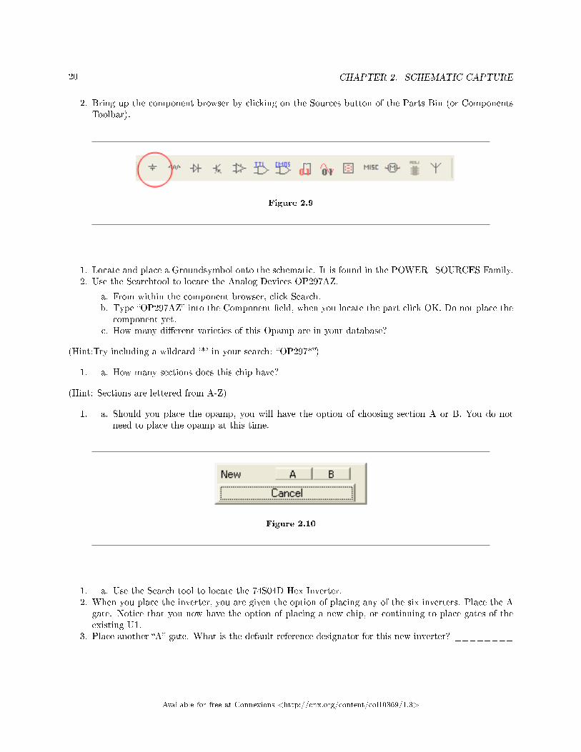
To access the Component Properties dialog box, double-click on a placed component, click on the Valuetab, and click the Edit Component in DB button (Figure 8).
Available for free at Connexions <http://cnx.org/content/col10369/1.3>

18 CHAPTER 2. SCHEMATIC CAPTURE
Figure 2.7: Component Wizard
Available for free at Connexions <http://cnx.org/content/col10369/1.3>
19
Figure 2.8: Component Properties Dialog Box
More details on creating custom components are available in the helples.
2.2 Exercise: Finding and Placing Components in National Instru-
ments Multisim2
2.2.1 Approximate time to complete: 10 minutes
This exercise has been designed to introduce users to the component browser. By the end of this exercise,you should be able to open the component browser, search and nd components that you need, and learnmore information about those components using the various elds of the browser.
2.2.2 Objectives
• Learn how to use the component browser to locate desired components.• Become familiar with the information that the component browser provides.
2.2.3 Procedure
1. Open a new schematic window (File/New/Schematic Capture).
2This content is available online at <http://cnx.org/content/m13739/1.1/>.
Available for free at Connexions <http://cnx.org/content/col10369/1.3>
20 CHAPTER 2. SCHEMATIC CAPTURE
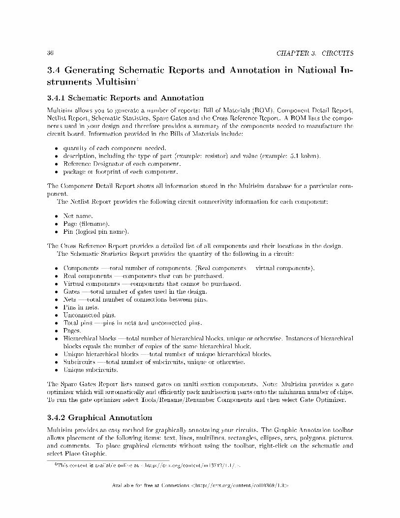
2. Bring up the component browser by clicking on the Sources button of the Parts Bin (or ComponentsToolbar).
Figure 2.9
1. Locate and place a Groundsymbol onto the schematic. It is found in the POWER_SOURCES Family.2. Use the Searchtool to locate the Analog Devices OP297AZ.
a. From within the component browser, click Search.b. Type OP297AZ into the Component eld, when you locate the part click OK. Do not place the
component yet.c. How many dierent varieties of this Opamp are in your database?__________
(Hint:Try including a wildcard `*' in your search: OP297*)
1. a. How many sections does this chip have? __________
(Hint: Sections are lettered from A-Z)
1. a. Should you place the opamp, you will have the option of choosing section A or B. You do notneed to place the opamp at this time.
Figure 2.10
1. a. Use the Search tool to locate the 74S04D Hex Inverter.2. When you place the inverter, you are given the option of placing any of the six inverters. Place the A
gate. Notice that you now have the option of placing a new chip, or continuing to place gates of theexisting U1.
3. Place another A gate. What is the default reference designator for this new inverter? ________
Available for free at Connexions <http://cnx.org/content/col10369/1.3>

21
2.3 Electrical and Electronic Component Manipulation in National
Instruments Multisim3
2.3.1 Component Placement, Rotation, Selection and Wiring
2.3.1.1 Placement, Rotation, and Selection
Once parts have been selected from their respective database, it is time to place them onto the schematic,and wire them together. Double-clicking on a component in the browser will attach that component to thecursor. This behavior is known as ghosting. Ghosting helps guide users when placing components anywhereon the schematic by left-clicking at the desired location.
Components can also be rotated while ghosting, and any time after placement. To rotate a part whileghosting, press Ctrl-R. Ctrl-R will also work when a placed component is selected. Placed components canalso be rotated by right-clicking on them and selecting 90 Clockwise or 90 CounterCW.
Figure 2.11: Component Rotation
3This content is available online at <http://cnx.org/content/m13734/1.1/>.
Available for free at Connexions <http://cnx.org/content/col10369/1.3>

22 CHAPTER 2. SCHEMATIC CAPTURE
Figure 2.12: Replacing Components
To select a component, simply-left click on it. To select multiple components, click and drag to create aselection around the desired components. A dashed line indicates that a component is selected. Individualelements of a symbol can also be selected, such as the component value and reference designator. To selectthese, left-click on the desired text or graphic element.
Holding the Shift key while selecting allows multiple components to be selected or de-selected.Components can be replaced by right-clicking on them then selecting Replace Component(s) from the
right-click menu. Users can then select the replacement components from the newly opened componentbrowser. Multisim will connect the new component to the same nets as the original component.
2.3.1.2 Wiring
Multisim provides modeless operation the action performed by the mouse cursor is dependent on thecursor's location. There is no need to select a tool, or mode when working with Multisim. The cursor willchange depending on what object is underneath it. describes the dierent icons that the mouse cursor willdisplay.
Available for free at Connexions <http://cnx.org/content/col10369/1.3>

23
When the cursor is over a pin or terminal of a component, that component can easily be wired byleft-clicking. When the cursor is over an existing wire and near a pin or terminal the net can easily bere-wired.
Left-click on the terminal to begin wiring, and to nish the wire, left-click on the destination terminal.When a wire is placed, Multisim will automatically assign it a net number. Net numbers increase
sequentially, beginning with 1. Ground nets are always numbered 0 a requirement of the underlyingSPICE simulator. To change a net number, or assign it a logical name instead, simply double-click on thewire.
Figure 2.13: Modeless Mouse Cursors
Available for free at Connexions <http://cnx.org/content/col10369/1.3>

24 CHAPTER 2. SCHEMATIC CAPTURE
Figure 2.14: Naming Nets
2.3.1.3 Autowiring by Touching Pins
Multisim also allows auto-connection of pins to wires, and pins to pins. To automatically connect a compo-nent to existing nets or pins, simply place that component so that its pins are touching an existing net orpin.
Available for free at Connexions <http://cnx.org/content/col10369/1.3>

25
Figure 2.15: Autowiring by Touching Pins
2.3.1.4 Autoconnect Passives
Multisim provides the ability to place a component in-line with an existing wire or set of wires. To automat-ically split an existing wire around a component, simply place that component in-line with the wire (Figure6).
Available for free at Connexions <http://cnx.org/content/col10369/1.3>

26 CHAPTER 2. SCHEMATIC CAPTURE
Figure 2.16: Autoconnect Passives
2.4 Exercise: Drawing A Schematic in National Instruments
Multisim4
2.4.1 Exercise: Drawing a Schematic in MultiSim
2.4.1.1 Approximate time to complete: 20 minutes.
This exercise provides a general introduction to Multisim's schematic capture. You will build and wire abasic circuit in Multisim using a variety of means to access parts, experiment with the wiring and run abasic simulation.
4This content is available online at <http://cnx.org/content/m13738/1.1/>.
Available for free at Connexions <http://cnx.org/content/col10369/1.3>

27
2.4.1.2 Objectives
• Understand the dierence between real, virtual, ideal, and interactive parts.• Build and wire a basic circuit (including virtual wiring).• Become familiar with and set wiring options.
2.4.1.3 Procedure
1. Build your own version of circuit 40kFILTER1_Complete.ms9 as pictured below. Select the requiredcomponents from the Master Database (Place/Component) and the In-Use List. Set component valuesas identied below. Note: Components R1, R2 and C2 are all virtual parts.
Figure 2.17: Bandpass Filter
1. To wire your circuit, point at a component terminal so that you see the cursor changes to crosshairs andleft-click. Move the pointer (while dragging the wire) to the second component terminal and left-clickto terminate.
2. Using the Replace function by right clicking on the R2, choose Replace Component(s) and substitutethe virtual resistor (R2) with a real resistor (Basic/Resistor) of your choice.
3. Double-click on the virtual components to see how they can be used to set variable parameters.4. Rotate and move a component within the circuit to see how movement of components aects the wiring.
Components can also be rotated while being placed from the database.5. Select the virtual capacitor from the In-Use List and place it between Points A and B in the circuit.
Notice the how it is automatically connected, and has a capacitance of 270 pF.
Available for free at Connexions <http://cnx.org/content/col10369/1.3>

28 CHAPTER 2. SCHEMATIC CAPTURE
SOLUTION5
5http://cnx.org/content/m13738/latest/40kFilter1_Complete.ms9
Available for free at Connexions <http://cnx.org/content/col10369/1.3>

Chapter 3
Circuits
3.1 Creating Circuits in Multisim1
3.1.1 Circuit Wizards
Multisim provides several circuit wizards, which can aid designers by quickly producing circuits to matchspecications. The circuits wizards provided are listed in . To use a circuit wizard, select Tools/CircuitWizards.
Figure 3.1: Circuit Wizards
1This content is available online at <http://cnx.org/content/m13731/1.2/>.
Available for free at Connexions <http://cnx.org/content/col10369/1.3>
29

30 CHAPTER 3. CIRCUITS
Figure 3.2: Filter Wizard Dialog Box
Use the 555 Timer Wizard to build astable and monostable oscillator circuits that use the 555 timer.The Multisim Filter Wizard helps design numerous types of lters by entering the specications into its
elds.The Common Emitter BJT Amplier Wizard helps design common emitter amplier circuits by entering
the desired specications into its elds. The Multisim MOSFET Amplier Wizard helps design MOSFETamplier circuits. The Multisim Opamp Wizard helps design the following opamp circuits. Users can enterthe desired specications in its elds:
• Inverting Amplier.• Non-inverting Amplier.• Dierence Amplier.• Inverted Summing Amplier.• Non-inverted Summing Amplier.• Scaling Adder.
Available for free at Connexions <http://cnx.org/content/col10369/1.3>

31
3.2 Using Electrical Rules Checking in National Instruments
Multisim2
3.2.1 Electrical Rules Check (ERC)
The Electrical Rules Check creates and displays a report detailing connection errors (such as an outputpin connected to a power pin) and unconnected pins. Once the circuit is wired, check the connections forcorrectness based on the rules set up in the Electrical Rules Check dialog box.
Depending on your circuit, you may wish to have warnings issued if some types of connections are present,error messages for other connection types, and no warnings or errors for other connections. You control thetype of connections that are reported when ERC is done by setting up the rules in the grid found in theERC Rules tab of the Electrical Rules Check dialog box.
ERC may be run over an entire design, or only across certain areas of a design. When an ERC is run,any anomalies are reported into a results pane at the bottom of the screen and the circuit is annotated withcircular error markers. Clicking on an error will center and zoom on the error location.
The ERC Options tab and ERC Rules tab are used to congure the ERC.To run the electrical rules check:1.Select Tools/Electrical Rules Check to display the Electrical Rules Check dialog box.2.Set up the reporting options using the ERC Options tab (Figure 1).3.Set up the rules using the ERC Options tab (Figure 2).4.Click OK. The results display in the format selected in the Output box in the ERC Options tab.
2This content is available online at <http://cnx.org/content/m13748/1.1/>.
Available for free at Connexions <http://cnx.org/content/col10369/1.3>

32 CHAPTER 3. CIRCUITS
Figure 3.3: ERC Options Tab
Available for free at Connexions <http://cnx.org/content/col10369/1.3>

33
Figure 3.4: ERC Rules Tab
3.3 Creating and Using Sub-Circuits in National Instruments
Multisim3
3.3.1 Sub-circuits and Hierarchical Blocks
Multisim provides the ability to handle increasingly complex designs. In addition to multi-sheet designs,users can create sub-circuits (SC), and hierarchical blocks (HB) to modularize repetitive circuits, or toabstract sophisticated designs.
Subcircuits are useful for compacting existing designs that would be best kept in a single le. Hierarchicalblocks are better suited for design reuse because they are stored in separate les and can be accessed forother designs.
Hierarchical blocks and subcircuits are functionally identical; the only dierence is in how their contentsare stored on disk.
Hierarchical blocks and subcircuits can be created using two methods, the rst method is to highlightan existing section of a circuit, and select Place/Connectors/HB/SC Connector. The second method isdescribed below.
3This content is available online at <http://cnx.org/content/m13733/1.1/>.
Available for free at Connexions <http://cnx.org/content/col10369/1.3>

34 CHAPTER 3. CIRCUITS
3.3.2 To place a new hierarchical block (2nd method):
1. Select Place/New Hierarchical Block and enter a lename.
Figure 3.5: Hierarchical Block Properties Dialog Box
or
1. Click on Browse, navigate to the folder where you would like to save the hierarchical block, enter aname and click Save. You are returned to the Hierarchical Block Properties dialog box.
2. Enter the number of pins desired and click OK. A ghost image of the new hierarchical block appears.Click where you want the hierarchical block to appear.
3. Double-click on the new hierarchical block and select Edit HB/SC from the HierarchicalBlock/Subcircuit dialog box that displays. A circuit window that contains only the entered pinsdisplays.
4. Place and wire components as desired in the new hierarchical block.5. Wire the hierarchical block into the circuit.6. Save the circuit.
Note: If you move or re-name a hierarchical block relative to the main circuit, Multisim will not be able tond it. A dialog box will ask you to provide the new location for the hierarchical block.
To place an existing hierarchical block from a le, select Place/Hierarchical Block from le and followthe same procedure.
3.3.3 To place a new subcircuit:
1. Select Place/New Subcircuit. The Subcircuit Name dialog box appears.
Available for free at Connexions <http://cnx.org/content/col10369/1.3>

35
Figure 3.6: Subcircuit Name Dialog Box
1. Enter the name you wish to use for the subcircuit, for example, PowerSupply and click OK. Yourcursor changes to a ghost image of the subcircuit indicating that the subcircuit is ready to be placed.
2. Click on the location in the circuit where you want the subcircuit placed (you can move it later, ifnecessary). The subcircuit appears in the desired location on the circuit window as an icon with thesubcircuit name inside it.
3. Double-click on the new subcircuit and select Edit HB/SC from the Hierarchical Block/Subcircuitdialog box that displays. An empty circuit window appears.
4. Place and wire components as desired in the new hierarchical block.5. Select Place/Connectors/HB/SC Connector, and place and wire the connector as desired. Repeat for
any other required Connectors. When you return to the main circuit, the symbol for the subcircuitwill include pins for the number of connectors that you added.
6. Wire the subcircuit into the circuit.
3.3.4 Replacing Components with Hierarchical Blocks or Subcircuits
Multisim allows users to easily replace existing components with a hierarchical block or subcircuit. Simplyselect the components which comprise the desired subcircuit or hierarchical block, and select Place/Replaceby Hierarchical Blockor Place/Replace by Subcircuit.
3.3.5 Spreadsheet View
The Spreadsheet View provides a global perspective on object properties. It allows fast advanced viewingand editing of parameters including component details such as footprints, Reference Designators, attributesand design constraints.
The Spreadsheet View can also be used to modify groups of components at a time. The view can besorted by any column in either ascending or descending order. You can also export the contents to MicrosoftExcel® for further reports.
Available for free at Connexions <http://cnx.org/content/col10369/1.3>
36 CHAPTER 3. CIRCUITS
3.4 Generating Schematic Reports and Annotation in National In-
struments Multisim4
3.4.1 Schematic Reports and Annotation
Multisim allows you to generate a number of reports: Bill of Materials (BOM), Component Detail Report,Netlist Report, Schematic Statistics, Spare Gates and the Cross Reference Report. A BOM lists the compo-nents used in your design and therefore provides a summary of the components needed to manufacture thecircuit board. Information provided in the Bills of Materials include:
• quantity of each component needed.• description, including the type of part (example: resistor) and value (example: 5.1 kohm).• Reference Designator of each component.• package or footprint of each component.
The Component Detail Report shows all information stored in the Multisim database for a particular com-ponent.
The Netlist Report provides the following circuit connectivity information for each component:
• Net name.• Page (lename).• Pin (logical pin name).
The Cross Reference Report provides a detailed list of all components and their locations in the design.The Schematic Statistics Report provides the quantity of the following in a circuit:
• Components total number of components. (Real components + virtual components).• Real components components that can be purchased.• Virtual components components that cannot be purchased.• Gates total number of gates used in the design.• Nets total number of connections between pins.• Pins in nets.• Unconnected pins.• Total pins pins in nets and unconnected pins.• Pages.• Hierarchical blocks total number of hierarchical blocks, unique or otherwise. Instances of hierarchical
blocks equals the number of copies of the same hierarchical block.• Unique hierarchical blocks total number of unique hierarchical blocks.• Subcircuits total number of subcircuits, unique or otherwise.• Unique subcircuits.
The Spare Gates Report lists unused gates on multi-section components. Note: Multisim provides a gateoptimizer which will automatically and eciently pack multisection parts onto the minimum number of chips.To run the gate optimizer select Tools/Rename/Renumber Components and then select Gate Optimizer.
3.4.2 Graphical Annotation
Multisim provides an easy method for graphically annotating your circuits. The Graphic Annotation toolbarallows placement of the following items: text, lines, multilines, rectangles, ellipses, arcs, polygons, pictures,and comments. To place graphical elements without using the toolbar, right-click on the schematic andselect Place Graphic.
4This content is available online at <http://cnx.org/content/m13742/1.1/>.
Available for free at Connexions <http://cnx.org/content/col10369/1.3>
37
Figure 3.7: Graphical Annotation Toolbar
3.4.3 Circuit Description Box
In addition to adding text to a particular portion of a circuit, you can add general descriptions to your circuitusing the Circuit Description Box. You can also place bitmaps, sound and video in the Circuit DescriptionBox.
The contents of the Circuit Description Box are viewed in the top pane of the Circuit Description Boxwindow (select View/Circuit Description Box). To edit the contents of the Circuit Description Box, selectTools/Description Box Editor.
3.4.4 Title Blocks
A powerful title block editor allows you to create customized title blocks. If desired, a title block can beincluded on every page of your design.
Various elds in the title block are automatically lled in depending upon the context and variousdocument properties. When designing the title block, you choose one of the pre-dened elds or a customeld. You choose appropriate fonts depending upon your language of preference. To edit an existing, or tocreate a new title block, select Tools/Title Block Editor.
Title blocks can include elements such as text, lines, arcs, Bezier curves, rectangles, ovals, arcs, bitmaps,and so on.
To place a title block, select Place/Title Block. The title block can be automatically placed in any cornerby right-clicking on the title block and selecting Move To. To populate elds of each title block, simplydouble-click the title block.
3.4.5 Schematic Transfer to Ultiboard and Other Packages
Multisim includes a single-click feature which will transfer the current design to an installed copy of Ultiboard.Select Transfer/Transfer to Ultiboardto initiate the PCB design process. Designs can be easily forward andback-annotated using the same Transfer menu.
In addition to a transfer mechanism between Multisim and Ultiboard, designers also have the option totransfer designs to one of several other PCB layout packages. Note: Transferring designs to 3rd party layoutpackages may require matching Multisim components to components in the database of the chosen PCBlayout program.
Available for free at Connexions <http://cnx.org/content/col10369/1.3>

38 CHAPTER 3. CIRCUITS
Available for free at Connexions <http://cnx.org/content/col10369/1.3>

Chapter 4
Simulation
4.1 Simulating Circuits using the SPICE in National Instruments
Multisim1
4.1.1 Simulation Overview
While a good design naturally follows from quality schematics, truly great designs can made with the helpof simulation. Multisim provides powerful simulation capabilities and features which are simply unavailablein other EDA packages.
Simulating a design can result in fewer design iterations and less chance of errors in the prototype stageof product development. When a design is simulated at the front end of the design process, the number ofdesign cycles can be signicantly reduced.
In addition to a world-class SPICE simulator, Multisim also includes XSPICE simulation, enabling fastsimulation of digital other components.
Patented co-simulation techniques allow designers to simulate VHDL modeled components along with therest of a circuit. With MultiMCU, certain microcontrollers can be simulated in the very same mixed-modeenvironment. MultiMCU is not available for all versions of Multisim.
4.1.2 Using the Interactive Simulator
To begin a simulation, ensure that the circuit has all the necessary prerequisites. All circuits must includea ground reference, and a source. Once the circuit is ready for simulation, click the Run / Stop Simulationbutton
Figure 4.1: Run/Stop Simulation Button
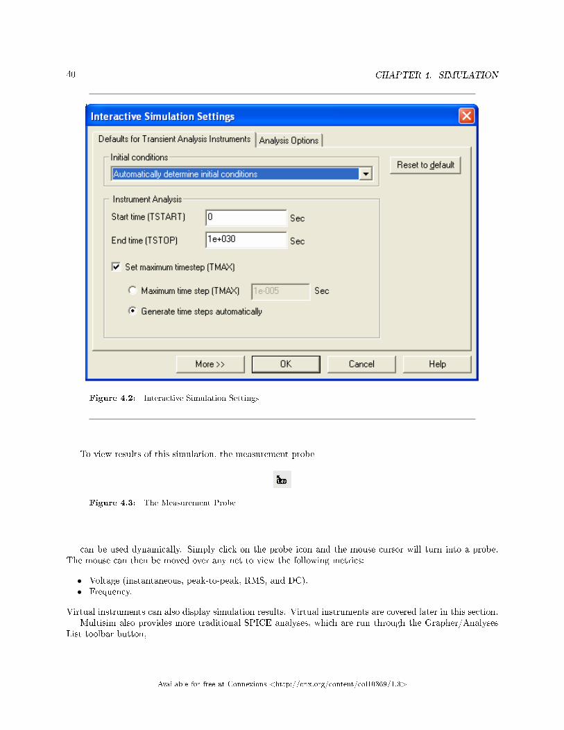
or press F5. An interactive circuit simulation will begin.The settings that are used for interactive simulation can be viewed and modied by selecting Simu-
late/Interactive Simulation Settings.Figure 1 below illustrates some of the settings available for interactivesimulation. The default end time for the simulation is 1e+30 seconds, or around 3.17e+30 billion years. Bydefault time steps will be generated automatically.
1This content is available online at <http://cnx.org/content/m13747/1.1/>.
Available for free at Connexions <http://cnx.org/content/col10369/1.3>
39
40 CHAPTER 4. SIMULATION
Figure 4.2: Interactive Simulation Settings
To view results of this simulation, the measurement probe
Figure 4.3: The Measurement Probe
can be used dynamically. Simply click on the probe icon and the mouse cursor will turn into a probe.The mouse can then be moved over any net to view the following metrics:
• Voltage (instantaneous, peak-to-peak, RMS, and DC).• Frequency.
Virtual instruments can also display simulation results. Virtual instruments are covered later in this section.Multisim also provides more traditional SPICE analyses, which are run through the Grapher/Analyses
List toolbar button,
Available for free at Connexions <http://cnx.org/content/col10369/1.3>

41
Figure 4.4: Grapher/Analyses List toolbar button
or by selecting Simulate/Analyses. Analyses are described in greater detail later in this section.
4.1.3 Handling Simulation Errors
Sooner or later, even the most experienced SPICE users will run into a SPICE simulation error. Multisimincludes a simulation advisor to help discover and x the source of troubling errors.
When an error message appears such as the one in Figure 5, click the Adviser button to access theavailable help.
Figure 4.5: Simulation Error Log Dialog Box
Available for free at Connexions <http://cnx.org/content/col10369/1.3>

42 CHAPTER 4. SIMULATION
Figure 4.6: Simulation Advisor
Two of the most often encountered errors are timestep errors, and singular matrix errors. below providesthe most common solutions to these simulation errors.
Available for free at Connexions <http://cnx.org/content/col10369/1.3>

43
Figure 4.7: Common Solutions to Simulation Errors
Available for free at Connexions <http://cnx.org/content/col10369/1.3>

44 CHAPTER 4. SIMULATION
4.2 Instrumenting a Circuit Simulation in National Instruments
Multisim2
4.2.1 Instrumenting a Simulation in MultiSim
Virtual instruments are components in Multisim which model real-world bench-top instruments. Examplesof virtual instruments in Multisim include Oscilloscopes, Function Generators, Network Analyzers, and BodePlotters.
Virtual instruments provide designers with an easy and intuitive method for interacting with their circuitsas they would in a testing or prototyping phase.
In addition to the provided virtual instruments, designers with familiar with National Instruments Lab-VIEW can create their own custom instruments from scratch. For example, one could create a custom noisegenerator to model electromagnetic interference.
Custom virtual instruments written in NI LabVIEW can also acquire real-world data and use the data todrive simulations, and can send generated data to analog output hardware, allowing simulated data to controlreal-world devices. The LabVIEW development suite is required to create custom LabVIEW instruments,but not necessary to run existing LabVIEW based instruments.
To place a virtual instrument, select the desired instrument from the Instruments toolbar (Figure 1).To view the front panel of the instrument, double-click on the instrument icon. Make connections to theterminals of the instrument icon as you would to any other component.
Multisim also provides designers with simulated benchtop instruments. These are instruments such asthe Tektronix TDS 2024 Oscilloscope. They will look and operate exactly according to the manufacturers'user manuals.
Figure 4.8: Instruments Toolbar
A single circuit can have multiple instruments attached to it, including (for most tiers) multiple instancesof the same instrument. In addition, each circuit window can have its own set of instruments. Each instanceof any instrument is congured and connected independently.
An overview of the more common instruments is included in this section. For more detailed informationon how to use each instrument, consult the Multisim User Guide or helple.
4.2.1.1 Multimeter
Use the multimeter to measure AC or DC voltage or current, and resistance or decibel loss between twonodes in a circuit. The multimeter is auto-ranging, so a measurement range does not need to be specied.Its internal resistance and current are preset to near-ideal values, which can be changed.
2This content is available online at <http://cnx.org/content/m13743/1.1/>.
Available for free at Connexions <http://cnx.org/content/col10369/1.3>

45
Figure 4.9: Multimeter Schematic Symbol
Figure 4.10: Multimeter Front Panel
4.2.1.2 Function Generator
The function generator is a voltage source that supplies sine, triangular or square waves. It provides aconvenient and realistic way to supply stimulus signals to a circuit. The waveform can be changed and itsfrequency, amplitude, duty cycle and DC oset can be controlled. The function generator's frequency rangeis great enough to produce conventional AC as well as audio- and radio-frequency signals.
The function generator has three terminals through which waveforms can be applied to a circuit. Thecommon center terminal provides a reference level for the signal.
Available for free at Connexions <http://cnx.org/content/col10369/1.3>

46 CHAPTER 4. SIMULATION
Figure 4.11: Function Generator Schematic Symbol
Figure 4.12: Function Generator Front Panel
4.2.1.3 Oscilloscopes
Multisim includes several varieties of oscilloscopes. All of the scopes can be controlled like real-world oscil-loscopes. Horizontal timing and vertical voltages parameters can be adjusted. Triggering levels, and typesare also selectable. Data from the Multisim-exclusive oscilloscopes is available in the Grapher after theinteractive simulation has completed by selecting View/Grapher.
Multisim provides the following oscilloscopes:
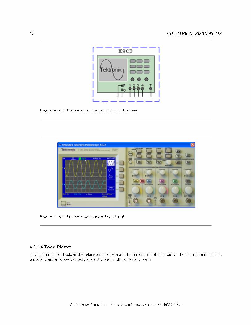
• 2-Channel.• 4-Channel.• Agilent 54622D Mixed Signal Oscilloscope.• Tektronix TDS 2024 Four Channel Digital Storage Oscilloscope.
Available for free at Connexions <http://cnx.org/content/col10369/1.3>
47
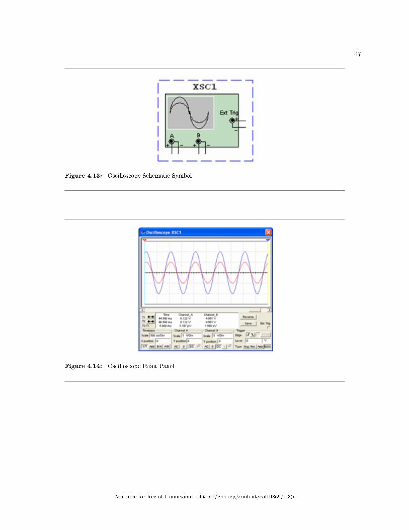
Figure 4.13: Oscilloscope Schematic Symbol
Figure 4.14: Oscilloscope Front Panel
Available for free at Connexions <http://cnx.org/content/col10369/1.3>
48 CHAPTER 4. SIMULATION
Figure 4.15: Tektronix Oscilloscope Schematic Diagram
Figure 4.16: Tektronix Oscilloscope Front Panel
4.2.1.4 Bode Plotter
The bode plotter displays the relative phase or magnitude response of an input and output signal. This isespecially useful when characterizing the bandwidth of lter circuits.
Available for free at Connexions <http://cnx.org/content/col10369/1.3>

49
Figure 4.17: Function Generator Schematic Symbol
Figure 4.18: Bode Plotter Front Panel
4.2.1.5 Spectrum Analyzer
The spectrum analyzer is used to measure amplitude versus frequency. This instrument is capable of mea-suring a signal's power and frequency components, and helps determine the existence of harmonics in thesignal.
The spectrum analyzer displays its measurements in the frequency domain rather than the time domain.Usually the reference frame in signal analysis is time. In that case, an oscilloscope is used to show theinstantaneous value as a function of time. Sometimes a sine waveform is expected but the signal, rather thanbeing a pure sinusoidal, has a harmonic on it. As a result, it is not possible to measure the waveform's level.If the same signal is displayed on a spectrum analyzer, its amplitude is displayed, along with its frequencycomponents, that is, its fundamental frequency and any harmonics it may contain.
Available for free at Connexions <http://cnx.org/content/col10369/1.3>

50 CHAPTER 4. SIMULATION
Figure 4.19: Spectrum Analyzer Schematic Symbol
Figure 4.20: Spectrum Analyzer Front Panel
4.3 Exercise: Instrumenting Simulated Circuits in National Instru-
ments Multisim3
4.3.1 Approximate time to complete: 20 minutes
This exercise will demonstrate the interactive simulator, and virtual instruments. By the end of this exercise,users will be familiar with placing instruments, opening their front panels, and conguring various options.
4.3.2 Objectives
• Learn how to place and connect virtual instruments.• Gain experience conguring instruments.
3This content is available online at <http://cnx.org/content/m13740/1.1/>.
Available for free at Connexions <http://cnx.org/content/col10369/1.3>

51
4.3.3 Procedure
1. Load circuit 40kFilter2.ms9 4 . Refer to while performing steps 2 - 4.2. Replace the Clock Source with a Function Generator. Once placed, double-click to open the instrument
panel and adjust its settings as follows:
• Waveform = sinewave• Amplitude = 1 V• Frequency = 40 kHz
1. Close the instrument panel.2. Attach the Bode plotter between the input and output nodes. Double-click to open the instrument
and adjust its settings as follows, then simulate and observe the output:
• Set Magnitude• Horizontal I (Initial) = 1 kHz, F (Final) = 1 MHz• Vertical I (Initial) = -50 dB, F (Final) = 10 dB
1. Attach an oscilloscope to monitor the input and output voltages.Double-click on the oscilloscope iconto adjust its settings as follows:
• Set Timebase = 20 us/Div• Channel A= 1 V/Div• Channel B = 1 V/Div
1. The color of the wire segment connected to an instrument controls the color of the trace on theinstrument display. Make sure that the wires from the output of the op-amp are blue. If they are not,then right-click on a wire segment and choose Wire Color to change the setting. Now, simulate andobserve the output.
2. Change the value of the Potentiometer (R3) by pressing A to increase the resistance and Shift-A todecrease the resistance during simulation. Observe the response on the oscilloscope. Note: The BodePlot response will be updated only after you re-simulate the circuit.
Figure 4.21
4http://cnx.org/content/m13740/latest/40kFilter2.ms9
Available for free at Connexions <http://cnx.org/content/col10369/1.3>

52 CHAPTER 4. SIMULATION
1. While the simulation is still running, use the Measurement Probe to view the voltage levels in thecircuit. It is found at the end of the instrument panel.
SOLUTION5
5http://cnx.org/content/m13740/latest/40kFilter2_Complete.ms9
Available for free at Connexions <http://cnx.org/content/col10369/1.3>

53
4.4 Creating LabVIEW Instruments to Instrument Circuit Simula-
tions in National Instruments Multisim6
6This content is available online at <http://cnx.org/content/m13732/1.1/>.
Available for free at Connexions <http://cnx.org/content/col10369/1.3>
54 CHAPTER 4. SIMULATION
4.4.1 Creating LabVIEW Instruments in MultiSim
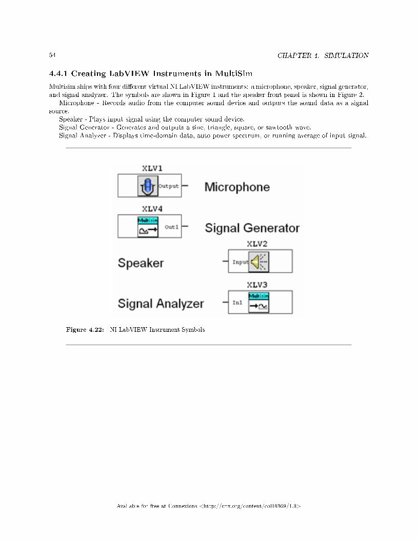
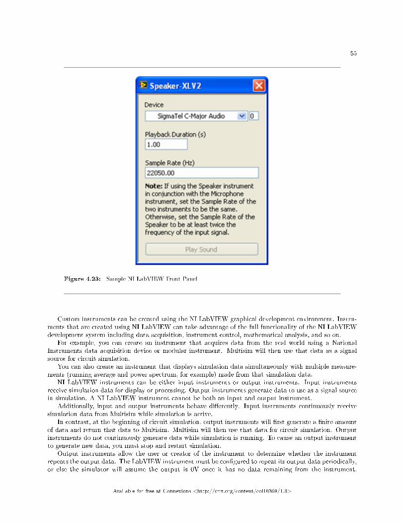
Multisim ships with four dierent virtual NI LabVIEW instruments: a microphone, speaker, signal generator,and signal analyzer. The symbols are shown in Figure 1 and the speaker front panel is shown in Figure 2.
Microphone - Records audio from the computer sound device and outputs the sound data as a signalsource.
Speaker - Plays input signal using the computer sound device.Signal Generator - Generates and outputs a sine, triangle, square, or sawtooth wave.Signal Analyzer - Displays time-domain data, auto power spectrum, or running average of input signal.
Figure 4.22: NI LabVIEW Instrument Symbols
Available for free at Connexions <http://cnx.org/content/col10369/1.3>
55
Figure 4.23: Sample NI LabVIEW Front Panel
Custom instruments can be created using the NI LabVIEW graphical development environment. Instru-ments that are created using NI LabVIEW can take advantage of the full functionality of the NI LabVIEWdevelopment system including data acquisition, instrument control, mathematical analysis, and so on.
For example, you can create an instrument that acquires data from the real world using a NationalInstruments data acquisition device or modular instrument. Multisim will then use that data as a signalsource for circuit simulation.
You can also create an instrument that displays simulation data simultaneously with multiple measure-ments (running average and power spectrum, for example) made from that simulation data.
NI LabVIEW instruments can be either input instruments or output instruments. Input instrumentsreceive simulation data for display or processing. Output instruments generate data to use as a signal sourcein simulation. A NI LabVIEW instrument cannot be both an input and output instrument.
Additionally, input and output instruments behave dierently. Input instruments continuously receivesimulation data from Multisim while simulation is active.
In contrast, at the beginning of circuit simulation, output instruments will rst generate a nite amountof data and return that data to Multisim. Multisim will then use that data for circuit simulation. Outputinstruments do not continuously generate data while simulation is running. To cause an output instrumentto generate new data, you must stop and restart simulation.
Output instruments allow the user or creator of the instrument to determine whether the instrumentrepeats the output data. The LabVIEW instrument must be congured to repeat its output data periodically,or else the simulator will assume the output is 0V once it has no data remaining from the instrument.
Available for free at Connexions <http://cnx.org/content/col10369/1.3>

56 CHAPTER 4. SIMULATION
Alternatively, if you congure the instrument and repeat the output data, the instrument will loop andrepeat its output periodically until the simulation has stopped.
Input instruments allow the user or creator of the instrument to set a sampling rate. This sampling rateis the rate at which the instrument receives data from Multisim. This sampling rate is analogous to thesampling rate you would set for a physical data acquisition device or modular instrument that acquires datafrom the real world. You should observe the Nyquist sampling theorem when choosing a sampling rate foryour instrument. Note that the higher the value of the sampling rate, the slower simulation will run.
To create and modify NI LabVIEW instruments, you must have the NI LabVIEW 8.0 (or later) Devel-opment System.
To use NI LabVIEW instruments, you must have the NI LabVIEW Run-Time Engine installed on yourcomputer. The version of this Run-Time Engine must correspond to the version of the NI LabVIEWDevelopment System used to create the instrument. The Multisim installer includes the NI LabVIEWRun-Time Engine 8.0 as part of the Electronics Workbench Shared Components installation.
4.5 Analyses of Circuit Simulations7
4.5.1 Analysis of Circuit Simulation
Multisim oers many analyses, all of which utilize simulation to generate the data for the desired analysis.These analyses range from quite basic to extremely sophisticated, and often require one analysis to beperformed as part of another. To congure and begin an analysis, select Simulate/Analyses, and choose thedesired analysis. Figure 1 lists all available Multisim analyses. For each analysis, you congure the settingsthat tell Multisim how to exactly perform the desired analysis. In addition to the analyses provided byMultisim, user-dened analyses can be created based on user-entered SPICE commands.
To prepare an analysis, congure the analysis-specic parameters, such as frequency range for an ACanalysis. Output traces must also be selected here. It is especially important to name nets appropriately toavoid confusion when analyzing results. The results are displayed on a plot in Multisim's Grapher and savedfor use in the Postprocessor. Some results are also written to an audit trail, which can be viewed.
7This content is available online at <http://cnx.org/content/m13730/1.2/>.
Available for free at Connexions <http://cnx.org/content/col10369/1.3>

57
Figure 4.24: Available Analyses
Available for free at Connexions <http://cnx.org/content/col10369/1.3>

58 CHAPTER 4. SIMULATION
Figure 4.25: AC Analysis Options Dialog Box
4.5.2 Grapher
The Grapher is the primary tool used to view the results of simulations. Users can view the Grapher byclicking View/Grapher. Additionally, the Grapher opens automatically displayed upon when running ananalysis. Elements of the Grapher window are detailed in Figure 3.
The display shows both graphs and charts. In a graph, data are displayed as one or more traces alongvertical and horizontal axes. In a chart, text data are displayed in rows and columns. The window is madeup of several tabbed pages, depending on how many analyses, etc. have been run.
Each page has two possible active areas which will be indicated by a red arrow: the entire page indicatedwith the arrow in the left margin near the page name or the chart/graph indicated with the arrow in the leftmargin near the active chart/graph. Some functions, such as cut/copy/paste, aect only the active area, sobe sure the desired area has been selected before performing a function.
Available for free at Connexions <http://cnx.org/content/col10369/1.3>

59
Figure 4.26: The Grapher
Through the properties pages, the Grapher provides extensive customization. Axes scales, ranges, titles,colors, line styles, and many more options can be modied. To access the page or standard properties pages,click Edit/Page Propertiesor Edit/Properties (Figure 4 and Figure 5).
Available for free at Connexions <http://cnx.org/content/col10369/1.3>

60 CHAPTER 4. SIMULATION
Figure 4.27: Grapher Page Properties
Figure 4.28: Graph Properties
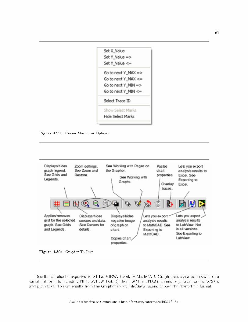
Cursors can be moved by clicking and dragging them with the mouse. Additionally, right-clicking on acursor, will display cursor movement options. Users can move the cursor to a particular X-Value, Y-Value,and local Maxima or Minima in either direction (Figure 6). Cursors, legends and graph lines can be toggledon or o by clicking the corresponding toolbar buttons (Figure 7).
Available for free at Connexions <http://cnx.org/content/col10369/1.3>
61
Figure 4.29: Cursor Movement Options
Figure 4.30: Grapher Toolbar
Results can also be exported to NI LabVIEW, Excel, or MathCAD. Graph data can also be saved to avariety of formats including NI LabVIEW Data (either .LVM or .TDM), comma separated values (.CSV),and plain text. To save results from the Grapher select File/Save As,and choose the desired le format.
Available for free at Connexions <http://cnx.org/content/col10369/1.3>

62 CHAPTER 4. SIMULATION
4.6 Exercise: Analysis of Circuit Simulations in National Instruments
Multisim8
4.6.1 Exercise: Working with Analyses in Circuit Simulation
4.6.1.1 Approximate time to complete: 35 minutes
In this exercise, users will further explore the characteristics of the bandpass lter using analyses. Userswill use AC, Transient, Fourier, and Monte Carlo Analyses and learn about analyses settings and how tocongure the Grapher.
4.6.1.2 Objectives
• Compare AC Analysis to a Bode plot• Compare Transient Analysis with the Oscilloscope• Use expressions in analyses• Understand how to set up and run Fourier Analysis• Understand how to set up tolerances and run a Monte Carlo Analysis• Learn how to format the output in the Grapher
4.6.1.3 Procedure
1. Load circuit 40kFilter3.ms9. 9 Notice that a load resistance has been added to the circuit (Rload) onthe output of the lter. This is to facilitate an output power analysis.
2. Run the Simulation to get the Bode plotter and oscilloscope traces. Double-click the Bode plotter andOscilloscope icons to open the instrument panels. Start the simulation by clicking on the lightning boltbutton, or by pressing F5. Stop the simulation after the Bode plot is displayed. Close the instrumentpanels by clicking on the Close button on each instrument. Note:You can also open and close instrumentpanels by double-clicking on the instrument icons.
3. Open the settings for an AC Analysis (Simulate/Analyses/AC Analysis).
a. On the Output tab, remove all variables from the Selected variables for analysis column on theright hand side of the dialog box. To do this, select all variables in the column and then clickRemove.
b. Select the $output variable and click Add.c. The test point will move to the right side under Selected Variables for Analysis.
4. Verify the output parameters and simulate.5. Click Simulate.
The Grapher appears with multiple tabs. The last three include: one for the oscilloscope, one for the Bodeplotter, and one for the AC Analysis. Compare the AC Analysis and the Bode Plotter graphs.
1. Perform the steps below to adjust the graph properties of the AC Analysis. These general steps canbe used for adjusting any graph.
2. Left-click on the Magnitude graph (top graph) to make it active.
A small arrow on the left side of the window indicates which graph is active.
1. Right-click on the left axis to access the Graph Properties option.
a. Select the Left Axis tab.
8This content is available online at <http://cnx.org/content/m13737/1.1/>.9http://cnx.org/content/m13737/latest/40kFilter3.ms9
Available for free at Connexions <http://cnx.org/content/col10369/1.3>

63
b. Enter the following information in the Left Axis tab:c. In the Scale box, choose Decibels.d. In the Label dialog, type Gain (dB).e. In the Axis box, choose Enabled and a Pen Size of 1.f. In the Range box, choose a minimum range of 50 and a maximum range of 10.
Figure 4.31: Setting the Graph Properties for the Magnitude
1. a. 1. In the Divisions section, choose Total Ticks of 4, Minor Ticks of 2 and Precision of 3.2. Click the Apply button.
b. Select the Bottom Axis tab.
1. Select Logarithmic Scale. In the Frequency Range, type 1000 for minimum and 1000000 formaximum.
2. Click Apply, then OK.
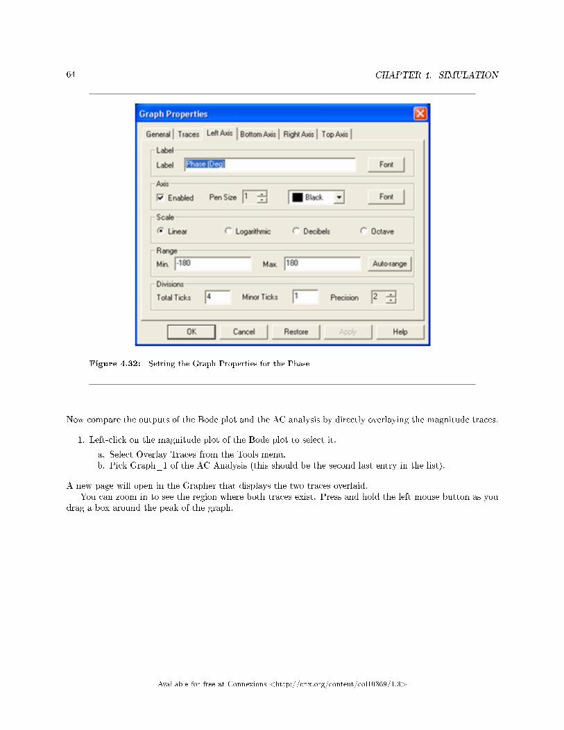
2. Adjust the bottom (Phase) graph by setting the Graph Properties as shown in the following gure.Then click on the Bottom Axis tab and change the range to 1000 to 1000000.
Available for free at Connexions <http://cnx.org/content/col10369/1.3>
64 CHAPTER 4. SIMULATION
Figure 4.32: Setting the Graph Properties for the Phase
Now compare the outputs of the Bode plot and the AC analysis by directly overlaying the magnitude traces.
1. Left-click on the magnitude plot of the Bode plot to select it.
a. Select Overlay Traces from the Tools menu.b. Pick Graph_1 of the AC Analysis (this should be the second last entry in the list).
A new page will open in the Grapher that displays the two traces overlaid.You can zoom in to see the region where both traces exist. Press and hold the left mouse button as you
drag a box around the peak of the graph.
Available for free at Connexions <http://cnx.org/content/col10369/1.3>

65
Figure 4.33: Zooming in on Overlaid Traces
Notice the results are slightly dierent. This is because the two methods used dierent sampling rates.You can control the sampling rate when you set up the instrument or the analysis.
1. Investigate how to make precise measurements in the Grapher.
a. Select the Bode Plot Tab in the Grapher.b. Turn on the cursors by selecting Show/Hide Cursors from the Viewmenu.c. Select one of the cursors and right-click on it.d. Select Go to next Y_MAX to nd the peak.e. Select Set Y_Value =>and enter the value that is 3 less than the max. This will give you one of
the -3dB points.f. Read the resulting value in the numeric display box.
2. Perform Transient Analysis (Simulate/Analyses/Transient Analysis).
a. Set the analysis settings as shown below. Note: You may need to expand the dialog box byclicking the More button.
Available for free at Connexions <http://cnx.org/content/col10369/1.3>
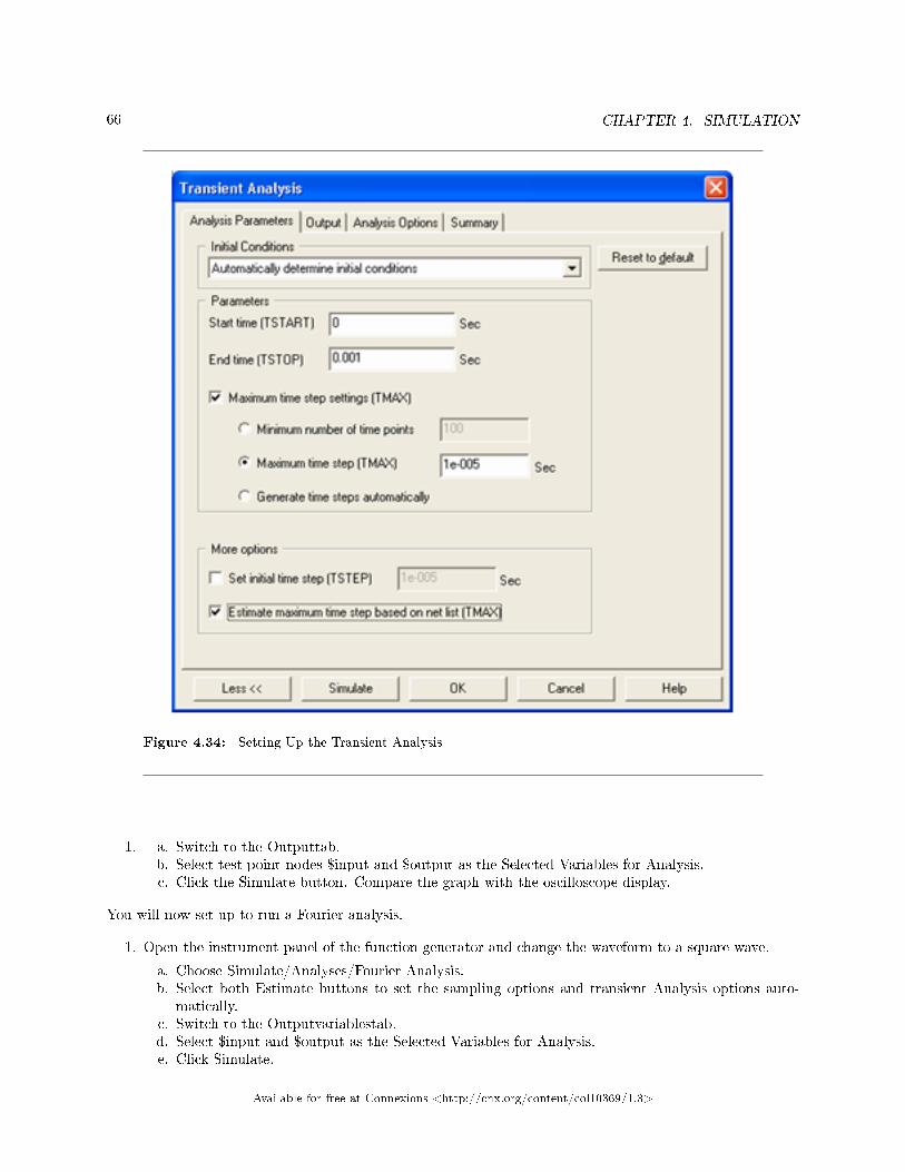
66 CHAPTER 4. SIMULATION
Figure 4.34: Setting Up the Transient Analysis
1. a. Switch to the Outputtab.b. Select test point nodes $input and $output as the Selected Variables for Analysis.c. Click the Simulate button. Compare the graph with the oscilloscope display.
You will now set up to run a Fourier analysis.
1. Open the instrument panel of the function generator and change the waveform to a square wave.
a. Choose Simulate/Analyses/Fourier Analysis.b. Select both Estimate buttons to set the sampling options and transient Analysis options auto-
matically.c. Switch to the Outputvariablestab.d. Select $input and $output as the Selected Variables for Analysis.e. Click Simulate.
Available for free at Connexions <http://cnx.org/content/col10369/1.3>

67
Note the output is presented on two separate pages in the Grapher.Optional Section (time permitting):Perform a Monte Carlo Analysis, (Simulate/Analyses/Monte Carlo).
1. From the front dialog box, select Add a new tolerance function.
a. In Parameter Type, choose Device Parameter.b. In Device Type select Capacitor. Choose cc1.c. In the Tolerance section, select Percent. For Tolerance Type, assign 20 and click Accept.
Figure 4.35: Setting Device Tolerances
1. a. Select Add a new tolerance again, and repeat the above procedure. Select cc2 this time.b. Now congure the Analysis Parameters.c. Click on the Analysis Parameters tab.d. Set it up to run an AC Analysis, with 5 runs, and set the Output variable to $output.e. Click on the Edit Analysis button and then congure the settings for the AC analysis.f. Set the FSTART to 1 kHz, the FSTOP to 1 MHz, the Number of points per decade to 100 andthe Vertical scale to Decibel.
g. Click the Simulate button.
Available for free at Connexions <http://cnx.org/content/col10369/1.3>

68 CHAPTER 4. SIMULATION
SOLUTION10
10http://cnx.org/content/m13737/latest/40kFilter3_Complete.ms9
Available for free at Connexions <http://cnx.org/content/col10369/1.3>

Chapter 5
Integrated Design and Academic
Features
5.1 Integrated Design with Multisim and Other National Instru-
ments Products1
5.1.1 Integrated Design with Other National Instruments Products
1This content is available online at <http://cnx.org/content/m13744/1.1/>.
Available for free at Connexions <http://cnx.org/content/col10369/1.3>
69

70 CHAPTER 5. INTEGRATED DESIGN AND ACADEMIC FEATURES
5.1.1.1 LabVIEW
National Instruments LabVIEW is a graphical programming environment that can be used to automate testand measurement functions, for the purpose of testing and validating designs. Multisim data saved in .LVMor .TDM format can be easily loaded into LabVIEW using express Virtual Instrument (VI) technology.Simulation data can then be overlaid on top of measured results to quickly and easily verify designs.
5.1.1.1.1 Loading .LVM and .TDM Data Files
To load Multisim simulated data that were saved in a .LVM or .TDM le, use the Read from MeasurementFile Express VI. This VI is located in the Programming/File IOpalette. For help on this le, consult theLabVIEW help le. The Express VI can be congured to read either .LVM or .TDM les.
Figure 5.1: Read from Measurement File Express VI
Note: The following only applies to .LVM les.The EOF? output terminal of the Express VI indicatestrue if there is more data contained in the .LVM le. This value is especially useful when reading data thatwere saved from a Bode Analysis, or from any plot window with more than one graph display. Simply placethe Read From Measurement File Express VI into a while loop, with the EOF? output terminal wired tothe exit condition terminal.
Note: The following only applies to .TDM les. To load .TDM les into LabVIEW which contain multiplegraphs, lower level storage express VIs are required. Figure 2 below gives a demonstration of how one mightload multiple graphs from a .TDM le.
Available for free at Connexions <http://cnx.org/content/col10369/1.3>

71
Figure 5.2: Loading Multiple Graphs from a .TDM File
Available for free at Connexions <http://cnx.org/content/col10369/1.3>

72 CHAPTER 5. INTEGRATED DESIGN AND ACADEMIC FEATURES
5.1.1.2 LabVIEW Based Virtual Instruments in Multisim
For further information on LabVIEW based Virtual Instruments in Multisim, consult the LabVIEW VirtualInstruments text in Section II.
5.1.1.3 SignalExpress
SignalExpress introduces an innovative approach to conguring your measurements using intuitive drag-and-drop steps that do not require code development. Unlike traditional benchtop measurement tools,SignalExpress combines the optimal balance of measurement functionality and ease-of-use to assist designersin streamlining a variety of applications:
• Design modeling.• Design verication.• Design characterization.• Device validation.• Automated test troubleshooting.
5.1.1.3.1 Loading Multisim Data into SignalExpress
To load simulated data into SignalExpress, simply use the Load from LVM step, selectAdd Step/Analog/Load and save Signals/Load from LVM. Choose the le name to load, and select thetraces to import. Use the Domain eld to choose from either Time, or Frequency data. Click close and runthe SignalExpress workbench le to load the Multisim data.
Available for free at Connexions <http://cnx.org/content/col10369/1.3>

73
Figure 5.3: SignalExpress Load from LVM Step
5.1.1.4 ELVIS
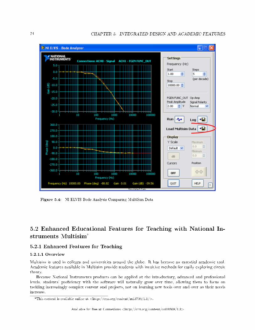
National Instruments ELVIS is an ideal companion to any electronics lab that uses Multisim. ELVIS providesa breadboard prototyping environment, with built-in instruments including a Function Generator, DigitalMultimeter (DMM), Oscilloscope, and Variable Power Supplies. The breadboard is detachable, allowingstudents to work on their projects and labs independently of the ELVIS unit.
ELVIS provides LabVIEW-based software for interacting with the Virtual Instruments. These instru-ments can be modied to load Multisim data for rapid comparison of simulated and measured data.
Available for free at Connexions <http://cnx.org/content/col10369/1.3>
74 CHAPTER 5. INTEGRATED DESIGN AND ACADEMIC FEATURES
Figure 5.4: NI ELVIS Bode Analysis Comparing MultiSim Data
5.2 Enhanced Educational Features for Teaching with National In-
struments Multisim2
5.2.1 Enhanced Features for Teaching
5.2.1.1 Overview
Multisim is used in colleges and universities around the globe. It has become an essential academic tool.Academic features available in Multisim provide students with intuitive methods for easily exploring circuittheory.
Because National Instruments products can be applied at the introductory, advanced and professionallevels, students' prociency with the software will naturally grow over time, allowing them to focus ontackling increasingly complex content and projects, not on learning new tools over and over as their needsincrease.
2This content is available online at <http://cnx.org/content/m13736/1.1/>.
Available for free at Connexions <http://cnx.org/content/col10369/1.3>

75
5.2.1.2 Prototyping
5.2.1.2.1 3D Virtual Components
Multisim includes a set of components specically designed for students with little to no experience workingwith parts in real life. When placed on the schematic, these 3D virtual components appear exactly as theylook in the real world. These components are available in the Basic group of the Master Database, underthe 3D_VIRTUAL family.
Figure 5.5: 3D Virtual Components
5.2.1.2.2 Animated Components
Animated components provide students with visual feedback on circuit operation during simulation. Exam-ples of animated components include LEDs, 7-Segment displays, and other interactive components such asswitches and potentiometers. Animated components are located throughout Multisim's databases.
5.2.1.2.3 Rated Components
Rated Componentshave tolerances just like real-world parts. Users can control the tolerance level by editingthe part properties. If the power being dissipated by a virtual rated resistor is above the threshold, theresistor will "explode" on the schematic, and act as an open circuit. Rated Virtualcomponents can be foundin the RATED_VIRTUAL family of the Basic group in the Master Database.
Available for free at Connexions <http://cnx.org/content/col10369/1.3>

76 CHAPTER 5. INTEGRATED DESIGN AND ACADEMIC FEATURES
5.2.1.2.4 3D Virtual Breadboard
Multisim also includes a 3D Virtual Breadboard. The breadboard can be used to teach students importantprototyping techniques. Nets and components will turn green on the schematic when their correspondingbreadboard elements have been correctly wired. The breadboard also includes a Design Rules Check (DRC)and Connectivity Check.
Figure 5.6: 3D Virtual Breadboard
5.2.1.2.5 3D Virtual ELVIS
In addition to the standard 3D Virtual Breadboard, students also have the option to create NI ELVISschematics, which will have a corresponding 3D ELVIS representation. The virtual instruments includedwith NI ELVIS such as the function generator, oscilloscope, and variable power supplies have also beenmodeled. To create an NI ELVIS schematic, click File/New/ELVIS Schematic.
To access the ELVIS virtual instruments, double-click on the terminals corresponding to the desiredinstrument.
Available for free at Connexions <http://cnx.org/content/col10369/1.3>

77
Figure 5.7: 3D NI ELVIS Schematic
Available for free at Connexions <http://cnx.org/content/col10369/1.3>

78 CHAPTER 5. INTEGRATED DESIGN AND ACADEMIC FEATURES
Figure 5.8: 3D Virtual NI ELVIS
5.2.1.3 Troubleshooting
5.2.1.3.1 Circuit Faults
Instructors have the ability to insert faults into schematics, and have students hone their troubleshootingskills by trying to nd the faults. The injected faults can be hidden to force students to apply fundamentaltechniques of troubleshooting. To add a fault into a component, double-click on the component, and selectthe Faults tab.
Faults include open circuits on a particular terminal, short circuits between two pins of a component,and resistive losses measured in Ohms.
Available for free at Connexions <http://cnx.org/content/col10369/1.3>
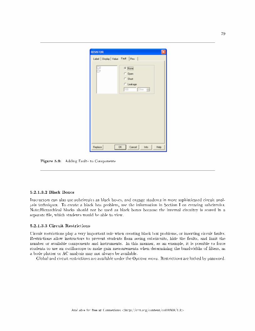
79
Figure 5.9: Adding Faults to Components
5.2.1.3.2 Black Boxes
Instructors can also use subcircuits as black boxes, and engage students in more sophisticated circuit anal-ysis techniques. To create a black box problem, use the information in Section I on creating subcircuits.Note:Hierarchical blocks should not be used as black boxes because the internal circuitry is stored in aseparate le, which students would be able to view.
5.2.1.3.3 Circuit Restrictions
Circuit restrictions play a very important role when creating black box problems, or inserting circuit faults.Restrictions allow instructors to prevent students from seeing subcircuits, hide the faults, and limit thenumber or available components and instruments. In this manner, as an example, it is possible to forcestudents to use an oscilloscope to make gain measurements when determining the bandwidths of lters, asa bode plotter or AC analysis may not always be available.
Global and circuit restrictions are available under the Options menu. Restrictions are locked by password.
Available for free at Connexions <http://cnx.org/content/col10369/1.3>

80 CHAPTER 5. INTEGRATED DESIGN AND ACADEMIC FEATURES
Figure 5.10: Circuit Restrictions Dialog Box
Available for free at Connexions <http://cnx.org/content/col10369/1.3>

ATTRIBUTIONS 81
Attributions
Collection: Introduction to Multisim Schematic Capture and SPICE Simulation
Edited by: Erik Luther, Janell RodriguezURL: http://cnx.org/content/col10369/1.3/License: http://creativecommons.org/licenses/by/2.0/
Module: "Objectives for the National Instruments Multisim Course"By: Janell RodriguezURL: http://cnx.org/content/m13746/1.1/Pages: 1-4Copyright: Janell RodriguezLicense: http://creativecommons.org/licenses/by/2.0/
Module: "Interactive Schematic Capture and Layout in National Instruments Multisim"By: Janell Rodriguez, Erik LutherURL: http://cnx.org/content/m13745/1.1/Pages: 4-9Copyright: Janell Rodriguez, Erik LutherLicense: http://creativecommons.org/licenses/by/2.0/
Module: "Exercise: Introducing the National Instruments Multisim Environment"By: Janell Rodriguez, Erik LutherURL: http://cnx.org/content/m13741/1.1/Pages: 9-10Copyright: Janell Rodriguez, Erik LutherLicense: http://creativecommons.org/licenses/by/2.0/
Module: "Electrical and Electronic Components Available in National Instruments Multisim"By: Janell Rodriguez, Erik LutherURL: http://cnx.org/content/m13735/1.1/Pages: 11-19Copyright: Janell Rodriguez, Erik LutherLicense: http://creativecommons.org/licenses/by/2.0/
Module: "Exercise: Finding and Placing Components in National Instruments Multisim"By: Janell Rodriguez, Erik LutherURL: http://cnx.org/content/m13739/1.1/Pages: 19-20Copyright: Janell Rodriguez, Erik LutherLicense: http://creativecommons.org/licenses/by/2.0/
Module: "Electrical and Electronic Component Manipulation in National Instruments Multisim"By: Janell Rodriguez, Erik LutherURL: http://cnx.org/content/m13734/1.1/Pages: 21-26Copyright: Janell Rodriguez, Erik LutherLicense: http://creativecommons.org/licenses/by/2.0/
Available for free at Connexions <http://cnx.org/content/col10369/1.3>

82 ATTRIBUTIONS
Module: "Exercise: Drawing A Schematic in National Instruments Multisim"By: Janell Rodriguez, Erik LutherURL: http://cnx.org/content/m13738/1.1/Pages: 26-28Copyright: Janell Rodriguez, Erik LutherLicense: http://creativecommons.org/licenses/by/2.0/
Module: "Creating Circuits in Multisim"By: Janell RodriguezURL: http://cnx.org/content/m13731/1.2/Pages: 29-30Copyright: Janell Rodriguez, Erik LutherLicense: http://creativecommons.org/licenses/by/2.0/
Module: "Using Electrical Rules Checking in National Instruments Multisim"By: Janell Rodriguez, Erik LutherURL: http://cnx.org/content/m13748/1.1/Pages: 31-33Copyright: Janell Rodriguez, Erik LutherLicense: http://creativecommons.org/licenses/by/2.0/
Module: "Creating and Using Sub-Circuits in National Instruments Multisim"By: Janell Rodriguez, Erik LutherURL: http://cnx.org/content/m13733/1.1/Pages: 33-35Copyright: Janell Rodriguez, Erik LutherLicense: http://creativecommons.org/licenses/by/2.0/
Module: "Generating Schematic Reports and Annotation in National Instruments Multisim"By: Janell Rodriguez, Erik LutherURL: http://cnx.org/content/m13742/1.1/Pages: 36-37Copyright: Janell Rodriguez, Erik LutherLicense: http://creativecommons.org/licenses/by/2.0/
Module: "Simulating Circuits using the SPICE in National Instruments Multisim"By: Janell Rodriguez, Erik LutherURL: http://cnx.org/content/m13747/1.1/Pages: 39-43Copyright: Janell Rodriguez, Erik LutherLicense: http://creativecommons.org/licenses/by/2.0/
Module: "Instrumenting a Circuit Simulation in National Instruments Multisim"By: Janell Rodriguez, Erik LutherURL: http://cnx.org/content/m13743/1.1/Pages: 44-50Copyright: Janell Rodriguez, Erik LutherLicense: http://creativecommons.org/licenses/by/2.0/
Module: "Exercise: Instrumenting Simulated Circuits in National Instruments Multisim"By: Janell Rodriguez, Erik LutherURL: http://cnx.org/content/m13740/1.1/Pages: 50-52Copyright: Janell Rodriguez, Erik LutherLicense: http://creativecommons.org/licenses/by/2.0/
Available for free at Connexions <http://cnx.org/content/col10369/1.3>

ATTRIBUTIONS 83
Module: "Creating LabVIEW Instruments to Instrument Circuit Simulations in National Instruments Mul-tisim"By: Janell Rodriguez, Erik LutherURL: http://cnx.org/content/m13732/1.1/Pages: 53-56Copyright: Janell Rodriguez, Erik LutherLicense: http://creativecommons.org/licenses/by/2.0/
Module: "Analyses of Circuit Simulations"By: Janell RodriguezURL: http://cnx.org/content/m13730/1.2/Pages: 56-61Copyright: Janell Rodriguez, Erik LutherLicense: http://creativecommons.org/licenses/by/2.0/
Module: "Exercise: Analysis of Circuit Simulations in National Instruments Multisim"By: Janell Rodriguez, Erik LutherURL: http://cnx.org/content/m13737/1.1/Pages: 62-68Copyright: Janell Rodriguez, Erik LutherLicense: http://creativecommons.org/licenses/by/2.0/
Module: "Integrated Design with Multisim and Other National Instruments Products"By: Janell Rodriguez, Erik LutherURL: http://cnx.org/content/m13744/1.1/Pages: 69-74Copyright: Janell Rodriguez, Erik LutherLicense: http://creativecommons.org/licenses/by/2.0/
Module: "Enhanced Educational Features for Teaching with National Instruments Multisim"By: Janell Rodriguez, Erik LutherURL: http://cnx.org/content/m13736/1.1/Pages: 74-80Copyright: Janell Rodriguez, Erik LutherLicense: http://creativecommons.org/licenses/by/2.0/
Available for free at Connexions <http://cnx.org/content/col10369/1.3>

Introduction to Multisim Schematic Capture and SPICE Simulation
This course introduces National Instruments Multisim through instructional modules and hands-on exercises.Multisim is an interactive, graphical schematic capture tool and SPICE simulator that allows you to buildcircuits, simulate, and instrument them in a virtual environment. Multisim has many enhanced featuresthat enhance the teaching of circuits and electronics concepts.
About Connexions
Since 1999, Connexions has been pioneering a global system where anyone can create course materials andmake them fully accessible and easily reusable free of charge. We are a Web-based authoring, teaching andlearning environment open to anyone interested in education, including students, teachers, professors andlifelong learners. We connect ideas and facilitate educational communities.
Connexions's modular, interactive courses are in use worldwide by universities, community colleges, K-12schools, distance learners, and lifelong learners. Connexions materials are in many languages, includingEnglish, Spanish, Chinese, Japanese, Italian, Vietnamese, French, Portuguese, and Thai. Connexions is partof an exciting new information distribution system that allows for Print on Demand Books. Connexionshas partnered with innovative on-demand publisher QOOP to accelerate the delivery of printed coursematerials and textbooks into classrooms worldwide at lower prices than traditional academic publishers.