Introduction to Multigrid Methods - Matematikcentrum · Introduction to Multigrid Methods ... Because r depends on y, this is the Explicit Euler method for y˙ = Mr(y) with step size

Introduction to Multigrid Methods

Chapter 8: Elements of Multigrid Methods

Gustaf Soderlind

Numerical Analysis, Lund University

Textbooks: A Multigrid Tutorial, by William L Briggs. SIAM 1988

A First Course in the Numerical Analysis of Differential Equations, by Arieh Iserles. Cambridge 1996

Matrix-based multigrid: Theory and Applications, by Yair Shapira. Springer 2008

Multi-Grid Methods and Applications, by Wolfgang Hackbusch, 1985

c⃝ Gustaf Soderlind, Numerical Analysis, Mathematical Sciences, Lund University, 2011-2012

Introduction to Multigrid Methods – p.1/61

1. Successive over-relaxation (SOR)

An attempt to speed up convergence in Gauss–Seidel

Du = Du− !(Au− f)

Du = Du− !(D − L− U)u+ !f

(D − !L)u =(

!U + (1− !)D)

u+ !f

(D − !L)um+1 =(

!U + (1− !)D)

um + !f

Iteration matrix PSOR = (D − !L)−1(

(1− !)D + !U)

Acceleration parameter ! = 1 ⇒ Gauss–Seidel method


Spectral radius of SOR matrix for TΔx

�[PSOR(!)] for N = 31, 63, 127

0 0.2 0.4 0.6 0.8 1 1.2 1.4 1.6 1.8 20.82

0.84

0.86

0.88

0.9

0.92

0.94

0.96

0.98

1

1.02Spectral radius vs omega

Acceleration paramter omega

Spec

tral r

adiu

s


Faster convergence is possible!

For 1D Poisson, the spectral radius is minimized at

! =2

1 +√

1− �2[PJ ]

As �[PJ ] = cos �Δx ≈ 1− �2Δx2/2 we have

! ≈ 2− 2�Δx

At this value the spectral radius of the SOR matrix is

�[PSOR(!)] = ! − 1 ≈ 1− 2�Δx

Much improved over Jacobi and Gauss–Seidel


SOR error sequence simulation

0 0.1 0.2 0.3 0.4 0.5 0.6 0.7 0.8 0.9 1−0.06

−0.04

−0.02

0

0.02

0.04

0.06

0.08

0.1Error in SOR at optimal omega

Note Error “transportation” in live demo!


SOR error sequence simulation, N = 99, 199

0 100 200 300 400 500 600 700 800 900 100010

−14

10−12

10−10

10−8

10−6

10−4

10−2

100

Convergence history SOR and GS

Err

or n

orm

Iteration number

Note Unit error reduction requires only O(N) iterations


2. Symmetric SOR (SSOR)

Neutralize “error transportation” to the left by alternatingbetween forward and backward sweeps

(D − !L)um+1 =(

!U + (1− !)D)

um + !f

(D − !U)um+2 =(

!L+ (1− !)D)

um+1 + !f

Iteration matrix PSORfwd = (D− !L)−1(

!U + (1− !)D)

andPSORbwd = (D − !U)−1

(

!L+ (1− !)D)

PSSOR = PSORbwdPSORfwd


SSOR error sequence simulation, N = 199

0 0.1 0.2 0.3 0.4 0.5 0.6 0.7 0.8 0.9 1−0.08

−0.06

−0.04

−0.02

0

0.02

0.04

0.06

0.08

0.1SSOR error simulation

Err

or

x

Note Error “transportation” eliminated


SSOR error sequence simulation, N = 199, 399

0 200 400 600 800 1000 1200 1400 1600 1800 200010

−14

10−12

10−10

10−8

10−6

10−4

10−2

100

Convergence history SSOR (b) and SOR (r)

Err

or n

orm

Iteration number

Note Unit error reduction in O(N) iterations, but SOR faster


SOR and SSOR spectral radii vs !

1 1.1 1.2 1.3 1.4 1.5 1.6 1.7 1.8 1.9 20.82

0.84

0.86

0.88

0.9

0.92

0.94

0.96

0.98

1

1.02Sectral radius for SOR (r) and SSOR (b)

Acceleration parameter omega

Spec

tral r

adiu

s

�[PSOR]√

�[PSORbwdPSORfwd] �[PSORbwdPSORfwd]

Note Optimal acceleration parameter ! does not move


3. Error diffusion and the Jacobi method

For the damped Jacobi method the error recursion is

em+1 = PJ(!)em

PJ(!) = (1− !)I + !PJ

Consider the diffusion equation yt = yxx with homogeneousboundary conditions and 2nd order MOL semidiscretization

y = TΔxy

Use explicit Euler time–stepping to get

ym+1 = ym +Δt ⋅ TΔxym


Jacobi and diffusion

Introduce the Courant number � = Δt/Δx2 and the Toeplitzmatrix

T =

⎛

⎜

⎜

⎜

⎜

⎜

⎝

−2 1 0

1 −2 1. . .

0 1 −2

⎞

⎟

⎟

⎟

⎟

⎟

⎠

The recursion becomes

ym+1 = ym + � ⋅ Tym


Jacobi and diffusion. . .

Split the matrix T = D − L− U = −2I + S and note that

S =

⎛

⎜

⎜

⎜

⎜

⎜

⎝

0 1 0

1 0 1. . .

0 1 0

⎞

⎟

⎟

⎟

⎟

⎟

⎠

= 2PJ

So the recursion can be written

ym+1 = ym + � ⋅ Tym =[

(1− 2�)I + 2�PJ

]

ym = PJ(2�)ym


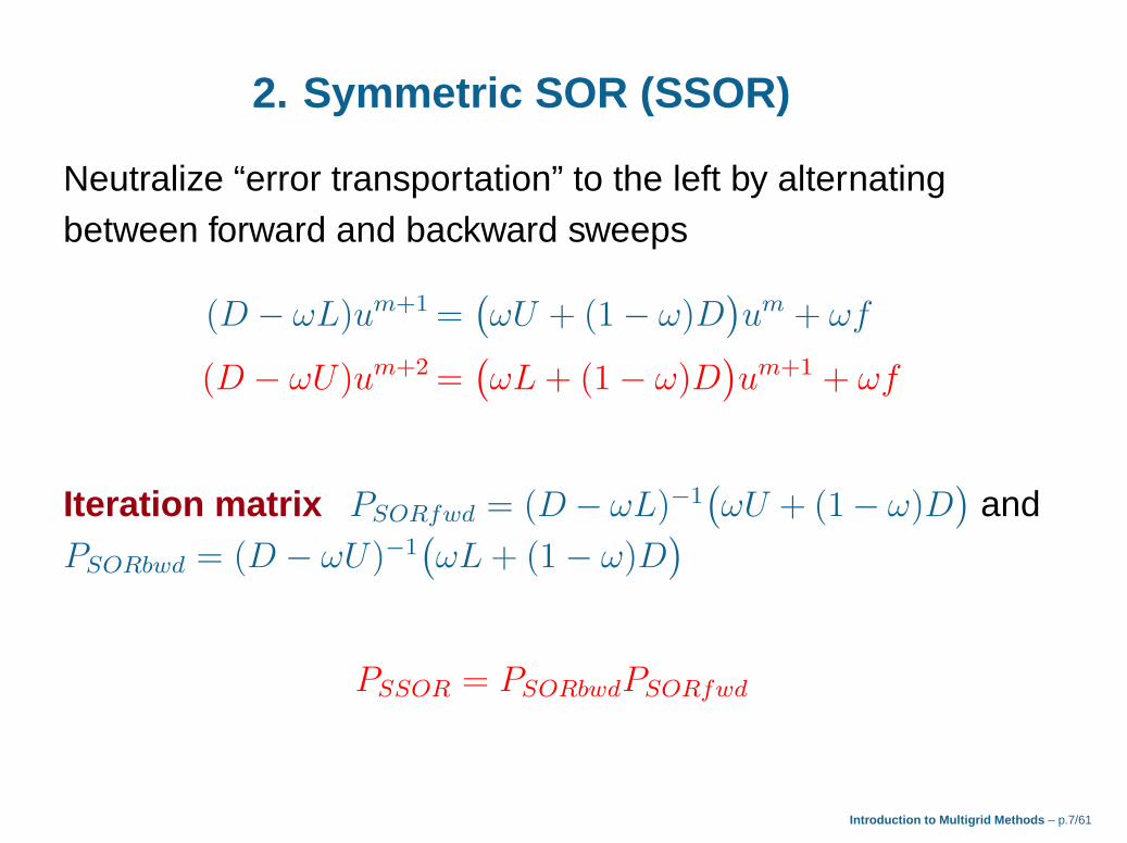
Error diffusion in the Jacobi method

Solving diffusion equation yt = yxx using Explcit Euler timestepping with finite difference MOL produces

ym+1 = PJ(2�)ym

Solving 2pBVP TΔxu = f using damped Jacobi iterationsproduces the error recursion

em+1 = PJ(!)em

The recursions are identical, with the interpretation twiceCourant number 2� = acceleration parameter !

Errors in damped Jacobi “diffuse” according to et = exx/2


Discrete diffusion

Explicit time-stepping for diffusion is extremely slowCFL condition 0 < � ≤ 1/2

The same thing will happen to Jacobi iterationsConvergence if 0 < ! ≤ 1

After many steps/iterations not on the CLF limit, the solutionwill approach the low frequency mode sin �x, while highfrequencies are efficiently damped

Recall What is a high frequency is a grid property


Side remark: The dynamic/static connection

If we want to solve the (dynamic) diffusion problem

yt = yxx − f(x)

its (static) stationary solution solves the 2pBVP

y′′ = f

When we try to solve the latter problem, every iterativemethod introduces (discrete) pseudo–dynamics

ym+1 = ym + !Mrm

Because r depends on y, this is the Explicit Euler method fory = Mr(y) with step size !


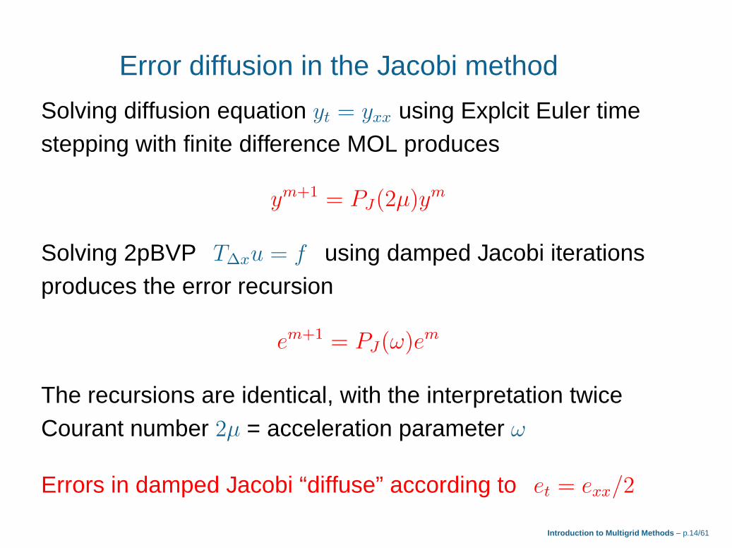
Summary of SOR methods

▶ Jacobi is diffusive in character, and Gauss–Seidel ishyperbolic/diffusive. Both require O(N 2) iterations for aunit error reduction

▶ SOR at optimal acceleration is largely hyperbolic incharacter and only requires O(N) iterations for a uniterror reduction

▶ Compare Δt/Δx2 and Δt/Δx CFL conditions

▶ SOR “transports” errors in space “accross boundary” withonly moderate damping along the way

▶ SSOR eliminates error “transportation” but is slower


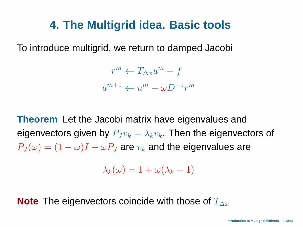
4. The Multigrid idea. Basic tools

To introduce multigrid, we return to damped Jacobi

rm ← TΔxum − f

um+1 ← um − !D−1rm

Theorem Let the Jacobi matrix have eigenvalues andeigenvectors given by PJvk = �kvk. Then the eigenvectors ofPJ(!) = (1− !)I + !PJ are vk and the eigenvalues are

�k(!) = 1 + !(�k − 1)

Note The eigenvectors coincide with those of TΔx


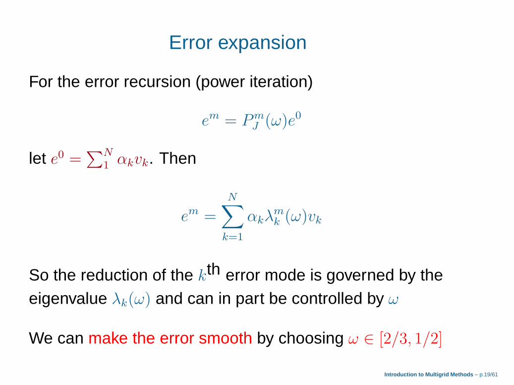
Error expansion

For the error recursion (power iteration)

em = PmJ (!)e0

let e0 =∑N

1�kvk. Then

em =

N∑

k=1

�k�mk (!)vk

So the reduction of the kth error mode is governed by theeigenvalue �k(!) and can in part be controlled by !

We can make the error smooth by choosing ! ∈ [2/3, 1/2]


Eigenvalue locations of PJ(!)

Eigenvalues for N = 31 and ! = 1, 0.5, 0.3, 0.2

0 0.5 1 1.5 2 2.5 3−1

−0.8

−0.6

−0.4

−0.2

0

0.2

0.4

0.6

0.8

1

k*pi*dx, for k=1:N, with N=31

Eig

en

valu

es

Eigenvalues of damped Jacobi matrix

High frequency damping can be controlled by !


Solution, Error and Residual

Given a linear system TΔxu = f construct sequence um → u

Now recall the following definitions

The Good The solution is defined by TΔxu = f

The Bad The error is defined by em = um − u

The Ugly The residual is defined by rm = TΔxum − f

TΔxem = rm


Error (defect) correction

Note that u = um − em. If we can estimate the error, e ≈ em,then

u← um − e

is an improved solution, so we can put um+1 ← um − e

Question Is it simpler to solve TΔxem = rm than TΔxu = f?

Answer YES! Because we only need moderate accuracy,solve the residual–error equation on coarse grid

This will still recover the persistent low frequency modes!


Error and residual

Recall

em =N∑

k=1

�k�mk (!)vk

with residual

rm = TΔxem =

N∑

k=1

�k�mk (!)�kvk

where �k is an eigenvalue of TΔx

Note As �k = −4

Δx2sin2 k�Δx

2the residual is huge


Error and residual. . .

Taking ! ∈ [2/3, 1/2] means that the error

em =

N∑

k=1

�k�mk (!)vk

is smooth, as only low frequency modes (�k ≈ 1) present

The residual is usually much less smooth because large �k

offset the benefit of small coefficients �k

Solve TΔxem = rm on a coarse grid

This still recovers low modes and converges faster


Example. Fine grid, coarse grid

Fine grid with an odd number N of internal grid points

Ωℎ = linspace(0,1,N+2)

ℎ = 1/(N + 1)

Coarse grid with (N − 1)/2 internal grid points

ΩH = linspace(0,1,(N+3)/2)

H = 2/(N + 1)

Mesh widths (step size) ℎ and H, respectively


Grid functions (vectors)

vℎ : Ωℎ → ℝ is a grid function with N components

It is an N–vector (excluding boundary points and data)

Compare a continuous function u : [0, 1]→ ℝ

Note u(Ωℎ) is the restriction of u to the grid Ωℎ

Let fℎ ≡ f(Ωℎ). If u′′ = f and Tℎvℎ = fℎ, the error is

eℎ = u(Ωℎ)− vℎ

Both the solution and the error are grid functions


Downsampling. From fine grid to coarse

Example Nℎ = 7 internal points on fine grid Ωℎ map toNH = 3 internal points on coarse grid via restriction map

vH =

⎛

⎜

⎜

⎝

0 1 0 0 0 0 0

0 0 0 1 0 0 0

0 0 0 0 0 1 0

⎞

⎟

⎟

⎠

vℎ = IHℎ vℎ

The restriction drops every second element. An alternative isa smoothing map, also known as a weighted restriction

vH =

⎛

⎜

⎜

⎝

1/4 1/2 1/4 0 0 0 0

0 0 1/4 1/2 1/4 0 0

0 0 0 0 1/4 1/2 1/4

⎞

⎟

⎟

⎠

vℎ


Smoothing map = plain restriction ∘ filter = IHℎ⋅ F�

⎛

⎜

⎜

⎝

1/4 1/2 1/4 0 0 0 0

0 0 1/4 1/2 1/4 0 0

0 0 0 0 1/4 1/2 1/4

⎞

⎟

⎟

⎠

=

⎛

⎜

⎜

⎝

0 1 0 0 0 0 0

0 0 0 1 0 0 0

0 0 0 0 0 1 0

⎞

⎟

⎟

⎠

⋅1

4

⎛

⎜

⎜

⎜

⎜

⎜

⎜

⎜

⎜

⎜

⎜

⎜

⎜

⎜

⎜

⎝

2 1 0 0 0 0 0

1 2 1 0 0 0 0

0 1 2 1 0 0 0

0 0 1 2 1 0 0

0 0 0 1 2 1 0

0 0 0 0 1 2 1

0 0 0 0 0 1 2

⎞

⎟

⎟

⎟

⎟

⎟

⎟

⎟

⎟

⎟

⎟

⎟

⎟

⎟

⎟

⎠


Mapping a fine grid function to a coarse

Example Sometimes one includes the boundary pointsNℎ = 3 internal points on fine grid Ωℎ map to NH = 1 internalpoint on coarse grid ΩH via restriction map

vH =

⎛

⎜

⎜

⎝

1 0 0 0 0

0 0 1 0 0

0 0 0 0 1

⎞

⎟

⎟

⎠

vℎ = IHℎ vℎ

A smoothing counterpart is (with unchanged boundaries)

vH =

⎛

⎜

⎜

⎝

1 0 0 0 0

0 1/4 1/2 1/4 0

0 0 0 0 1

⎞

⎟

⎟

⎠

vℎ


What is a digital filter?

Example To filter out HF, repeated averaging can be used

u =1

4

⎛

⎜

⎜

⎜

⎜

⎜

⎝

2 1 0 0

1 2 1 0

0 1 2 1

0 0 1 2

⎞

⎟

⎟

⎟

⎟

⎟

⎠

v = F� ⋅ v

Then u is smoother than v, F� is a 2nd order lowpass filter

Note The filter F� is Toeplitz or a discrete convolution, and

F� = (1−1

2)I +

1

2PJ = PJ(1/2)

Same as ! = 1/2 damped Jacobi iteration matrix for TΔx


Filters. Analogue and Digital

An analogue linear filter is an integral operator F : v 7→ u

u = Fv ⇔ u(x) =

∫ 1

0

f(x, y)v(y) dy

Its discrete counterpart is a digital filter

u = Fv ⇔ ui =

N∑

j=1

fi,jvj

The operator F (as defined by the kernel function f(x, y) andthe matrix {fi,j}) determine the filter characteristics


Convolutions and Toeplitz filters

A convolution filter is an integral operator F : v 7→ u

u = Fv ⇔ u(x) =

∫ 1

0

f(x− y) v(y) dy

A discrete convolution is of the form

u = Fv ⇔ ui =N∑

j=1

fi−jvj

Note F is a Toeplitz matrix, because if i− j = const thenfi,j = fi−j = const. Elements are diagonalwise constant

Theorem A Toeplitz filter is a discrete convolution


Oversampling. From coarse grid to fine

Note The maps IHℎ do not have inverses (information loss)

IℎH is an interpolation operator generating new elements

Left and right inverses

IℎH ⋅ IHℎ ∕= I

IHℎ ⋅ IℎH = I

The second identity holds if IHℎ is a plain restriction, but not ifit is a smoothing operator


Prolongation through linear interpolation

Example The interpolation operator IℎH can be defined bypiecewise linear interpolation

vj+1/2 ← (vj + vj+1)/2

This defines a prolongation of the grid function by inserting aninterpolated value between previous coarse grid points

Other types of interpolation, such as splines, are possible butare often too expensive and of little advantage

Choose linear interpolation with linear FEM basis functions


Matrix representation of the prolongation

Example Prolongation from 3 internal points to 7

vℎ =

⎛

⎜

⎜

⎜

⎜

⎜

⎜

⎜

⎜

⎜

⎜

⎜

⎜

⎜

⎜

⎝

1/2 0 0

1 0 0

1/2 1/2 0

0 1 0

0 1/2 1/2

0 0 1

0 0 1/2

⎞

⎟

⎟

⎟

⎟

⎟

⎟

⎟

⎟

⎟

⎟

⎟

⎟

⎟

⎟

⎠

vH = IℎHvH

Compare using smoothing restriction: IℎH = 2F�(IHℎ )T


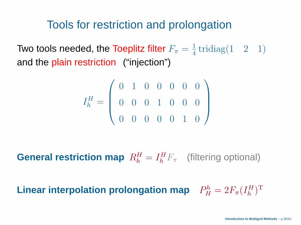
Tools for restriction and prolongation

Two tools needed, the Toeplitz filter F� = 1

4tridiag(1 2 1)

and the plain restriction (“injection”)

IHℎ =

⎛

⎜

⎜

⎝

0 1 0 0 0 0 0

0 0 0 1 0 0 0

0 0 0 0 0 1 0

⎞

⎟

⎟

⎠

General restriction map RHℎ = IHℎ F� (filtering optional)

Linear interpolation prolongation map P ℎH = 2F�(I

Hℎ )T


5. A simple two-grid iteration

Solve Tℎuℎ = fℎ iteratively using the following algorithm

1. Run one damped ! = 2/3 Jacobi iteration on fine grid

um+1

ℎ ← umℎ − !D−1

ℎ rmℎ m = 0 : M − 1

2. Compute residual and restrict rH ← IHℎ F�(TℎuMℎ − fℎ)

3. Solve error equation THeH = rH

4. Prolong eMℎ ← IℎHeH

5. Correct uM+1

ℎ ← uMℎ − eMℎ

6. Run one damped Jacobi iteration on fine grid

7. Repeat from 1 until convergence


MATLAB code segment: the two-grid V step

rf = Tdx*v - f; % Compute residualv = v - omega*Ddx∖rf; % Pre-smoothing Jacobi

rf = Tdx*v - f; % Compute residualrf = lowpass(rf); % Optional LP filter

rc = FMGrestrict(rf); % Restrict to coarse gridec = Tdxc∖rc; % Solve error equationef = FMGprolong(ec); % Prolong to fine grid

v = v - ef; % Correct: remove error

rf = Tdx*v - f; % Compute residualv = v - omega*Ddx∖rf; % Post-smoothing Jacobi


Numerical test: Two-grid method, N = 2048

0 0.2 0.4 0.6 0.8 1−0.1

0

0.1

0.2

0.3

0.4Exact (g) & initial approx (b)

0 0.2 0.4 0.6 0.8 110

−20

10−15

10−10

10−5

100

Error estimate progression

0 0.2 0.4 0.6 0.8 1−6

−4

−2

0

2x 10

−7 Remaining errors

0 0.2 0.4 0.6 0.8 1−0.1

0

0.1

0.2

0.3

0.4Exact (g) & numerical (b)

4 V-cycles on u′′ = f on on fine grid with 2048 points, errorestimation on 1024, single PJ(1/2) pre- and post-smoothing



0 0.2 0.4 0.6 0.8 1−0.1

0

0.1

0.2

0.3


0 0.2 0.4 0.6 0.8 110

−15

10−10

10−5

100


0 0.2 0.4 0.6 0.8 1−4

−3

−2

−1

0

1

2x 10


0 0.2 0.4 0.6 0.8 1−0.1

0

0.1

0.2

0.3





0 0.2 0.4 0.6 0.8 1−0.1

0

0.1

0.2

0.3


0 0.2 0.4 0.6 0.8 110

−8

10−6

10−4

10−2

100


0 0.2 0.4 0.6 0.8 1−2.5

−2

−1.5

−1

−0.5

0

0.5

1x 10


0 0.2 0.4 0.6 0.8 1−0.1

0

0.1

0.2

0.3





0 0.2 0.4 0.6 0.8 1−0.1

0

0.1

0.2

0.3


0 0.2 0.4 0.6 0.8 110

−8

10−6

10−4

10−2

100


0 0.2 0.4 0.6 0.8 1−1

−0.5

0

0.5

1x 10


0 0.2 0.4 0.6 0.8 1−0.1

0

0.1

0.2

0.3


4 V-cycles on u′′ = f on on fine grid with 256 points, errorestimation on 128, with initial data contaminated by noise



0 0.2 0.4 0.6 0.8 1−0.1

0

0.1

0.2

0.3


0 0.2 0.4 0.6 0.8 110

−6

10−4

10−2

100


0 0.2 0.4 0.6 0.8 1−2.5

−2

−1.5

−1

−0.5

0

0.5

1x 10


0 0.2 0.4 0.6 0.8 1−0.1

0

0.1

0.2

0.3


4 V-cycles on u′′ = f on on fine grid with 32 points, errorestimation on 16, with initial data contaminated by noise


Observations in the numerical tests

▶ One can almost use the same number of iterations

▶ By and large, convergence is unaffected by Δx→ 0

▶ One can solve the problem to high accuracy so that onlythe global error remains

▶ The basic iterative method is not crucial but must besmoothing

▶ Large initial errors are not a problem

▶ The method is robust even with respect to noise


Why is the Multigrid Method faster?

All iterative methods work with the residual

ym+1 = ym + !Mrm

The difference is that multigrid estimates the error

▶ The residual is large and nonsmooth

▶ The error is moderate and smooth

▶ Basic residual-reducing iterative methods typically fail toeliminate low frequency error components

▶ Therefore only error estimating methods can be fast


6. Multigrid on nested grids. The V cycle

We want to solve TKuK = fK on a fine grid ΩK with meshwidth ℎK

Construct an embeddeding of grids Ω0 ⊂ Ω1 ⊂ ⋅ ⋅ ⋅ ⊂ ΩK withmesh widths ℎ0 > ℎ1 > ⋅ ⋅ ⋅ > ℎK

On regular grids one typically takes ℎk = 2ℎk+1 to makerestrictions and prolongations simple

We want to formulate multigrid methods for solving

TKuK = fK

on ΩK using all available grids


Assumptions

▶ There are restriction operators Ik−1

k : Ωk → Ωk−1

▶ There are prolongation operators Ik+1

k : Ωk → Ωk+1

▶ The restrictions and prolongations must be very fast andrun in O(N) operations

▶ There is an iterative method with the smoothing propertyon every grid Ωk, i.e., it must attenuate high frequenciesby a constant factor independently of ℎk

▶ T0u0 = f0 can be solved fast to provide a crude estimateu0


The operators {Tk}

Different operators Tk are needed on the different gridsStandard approach: if possible use same discretization

It may be “difficult” to construct the Tk

Use restriction and prolongation operators!

Definition The operator triple (Tk, Rk−1

k , P kk−1) satisfies

the Galerkin condition if

Tk−1 = Rk−1

k TkPkk−1

where Rk−1

k is the restriction and P kk−1 is the prolongation


The V-cycle. Sweep through the grids

Obtain a starting approximation by solving the problem on avery coarse grid, typically Ω0. Solving means by directmethod, N = 1000 could be typical. Prolong to finest grid

A “V” sweep Iterate from finest grid on successively coarsergrids down to Ω0, then back to ΩK on successively finer grids

Repeat V-sweeps to form a “V–cycle” and iterate untilconvergence

Visit enough grids (many) to suppress the entire spectrum offrequencies, coarse grids for slow, fine grids for fast


A full, recursive multigrid V-cycle

1. Procedure v := FMGV (vk, Tk, fk)

2. If k = 0 return v ← T0∖f0 and STOP else:

3. Pre-smoothing vk ← vk − !D−1

k (Tkvk − fk)

4. Restrict residual to coarse grid rk−1 ← Ik−1

k (Tkvk − fk)

5. Recursive error estimation ek−1←FMGV (0, Tk−1, rk−1)

6. Prolong error to fine grid ek ← Ikk−1ek−1

7. Correct by removing error vk ← vk − ek

8. Post-smoothing vk ← vk − !D−1

k (Tkvk − fk)

9. Output v ← vk


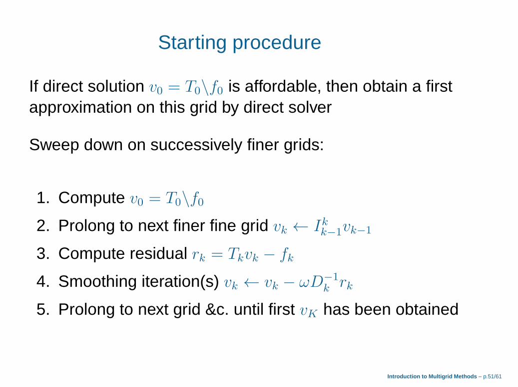
Starting procedure

If direct solution v0 = T0∖f0 is affordable, then obtain a firstapproximation on this grid by direct solver

Sweep down on successively finer grids:

1. Compute v0 = T0∖f0

2. Prolong to next finer fine grid vk ← Ikk−1vk−1

3. Compute residual rk = Tkvk − fk

4. Smoothing iteration(s) vk ← vk − !D−1

k rk

5. Prolong to next grid &c. until first vK has been obtained


MATLAB code segment. The recursive V cycle

rf = Tdx*v - f; % Compute residualv = v - omega*Ddx∖rf; % Pre-smoothing Jacobi

rf = Tdx*v - f; % Compute residualrf = lowpass(rf); % Optional LP filter

rc = FMGrestrict(rf); % Restrict to coarseec = FMGV(0,T2dx,rc); % Solve error equationef = FMGprolong(ec); % Prolong to fine grid

v = v - ef; % Correct: remove error

rf = Tdx*v - f; % Compute residualv = v - omega*Ddx∖rf; % Post-smoothing Jacobi


Numerical test: Full MG V-cycles, N = 63

0 0.1 0.2 0.3 0.4 0.5 0.6 0.7 0.8 0.9 110

−6

10−5

10−4

10−3

10−2

Error progression

0 0.1 0.2 0.3 0.4 0.5 0.6 0.7 0.8 0.9 1−0.1

0

0.1

0.2

0.3

0.4Solution: exact (g), numerical (b), err/dx2/10 (r)

6 V-cycles on u′′ = f on on fine grid with 63 points, coarsestgrid with 31 points and Jacobi ! = 2/3



0 0.1 0.2 0.3 0.4 0.5 0.6 0.7 0.8 0.9 110

−10

10−8

10−6

10−4

10−2

Error progression

0 0.1 0.2 0.3 0.4 0.5 0.6 0.7 0.8 0.9 1−0.1

0

0.1

0.2

0.3





0 0.1 0.2 0.3 0.4 0.5 0.6 0.7 0.8 0.9 110

−15

10−10

10−5

100

Error progression

0 0.1 0.2 0.3 0.4 0.5 0.6 0.7 0.8 0.9 1−0.1

0

0.1

0.2

0.3




Observations in the numerical tests

▶ By and large, multigrid iteration convergence isunaffected by Δx→ 0

▶ One can solve the problem to high accuracy so that onlythe global error remains

▶ Within 6 V-cycles the global error is reached

▶ Solution accuracy is O(Δx2)

▶ Large initial errors are not a problem

▶ The method is robust even with respect to noise, butmore V-cycles may be required for large N


7. Efficiency. Memory and execution time

Let the Kth grid have N internal points

Then grid K − 1 has (N + 1)/2− 1 < N/2 internal points

Total storage requirement is therefore

S = N ⋅ (1 + 2−1 + ⋅ ⋅ ⋅ + 2−K) < 2N

So, independently of the # of grids (recursion depths) storagedoes not exceed that of using a single finer mesh


Memory requirements in d dimensions

Let the Kth grid have Nd points (curse of dimensions)

Then grid K − 1 has (N + 1)d/2− 1 < (N/2)d points

Total storage requirement in d dimensions is

Sd < Nd ⋅ (1 + 2−d + ⋅ ⋅ ⋅ + 2−dK) ≈ Nd

S1 < 2N S2 <4N 2

3S3 <

8N 3

7

So, for once, the curse of dimensions works our way!Multigrid is always cheaper than using a single finer grid


Execution time “in theory”

Work unit UK is the cost of one sweep on the fine Kth gridW0 ∼ 2−dKN 2d is cost for direct solution on coarsest grid

Neglect restriction and prolongation costs

Cost W of V cycle with one pre- and one post-smoothing

Wd < 2UK ⋅ (1 + 2−d + ⋅ ⋅ ⋅ + 2−dK) + 2W0 ≈ 2UK + 2W0

W1 < 4UK + 2W0 ; W2 <8UK

3+ 2W0 ; W3 <

16UK

7+ 2W0

So, execution time does not exceed that of a single sweep onthe next finer grid


So it’s cheap, what accuracy do we get?

Solving TΔxuΔx = f we obtain vΔx with

Algebraic error eΔx = uΔx − vΔx

Global error gΔx = uΔx − u(ΩΔx)

Total error �Δx = vΔx − u(ΩΔx)

Note that �Δx = gΔx − eΔx, therefore

∥vΔx − u(ΩΔx)∥Δx ≤ ∥uΔx − u(ΩΔx)∥Δx + ∥vΔx − uΔx∥Δx

≤ C ⋅Δx2 + "MG

Try to make "MG ≈ C ⋅Δx2 then global error will dominate


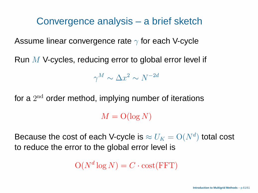
Convergence analysis – a brief sketch

Assume linear convergence rate for each V-cycle

Run M V-cycles, reducing error to global error level if

M ∼ Δx2 ∼ N−2d

for a 2nd order method, implying number of iterations

M = O(logN)

Because the cost of each V-cycle is ≈ UK = O(Nd) total costto reduce the error to the global error level is

O(Nd logN) = C ⋅ cost(FFT)


Documents

Introduction to Multigrid Methods - Matematikcentrum · Introduction to Multigrid Methods ... Because r depends on y, this is the Explicit Euler method for y˙ = Mr(y) with step size