Introduction to Modeling and Control of Internal Combustion Engine Systems Volume 28 || Control of Engine Systems

4

Control of Engine Systems

As discussed in the preceding chapters, engine systems contain a large num-ber of control loops. For the design of these feedforward and feedback controlsystems, the main objectives are:

• The driver’s demands for immediate torque response, good drivability, andlow fuel consumption must be met.

• The engine must be kept in a safe operating region where damage to orfatigue of the material is avoided. Knocking must be prevented, the catalyticconverter must not overheat, etc.

• The emission limits must be met. In the case of SI engines, this requiresa rapid light-off of the catalytic converter, precise stationary air/fuel ratiocontrol, and good compensations of the transient phenomena.

Since these requirements are partially contradictory, they must be fulfilled ac-cording to the priorities set by legislation and customer demands. In this op-timization, control systems play a major role as enabling technology.

The complete treatment of all control problems arising in engine systemsis beyond the scope of this text. The following five important case studies arepresented with the intention to show how model-based methods can be used tostreamline the design process:

• Physics-based modeling and control of engine knock as an example formodel-based signal processing, Sec. 4.2

• The air/fuel-ratio control as a typical combined feedforward and feedbackcontrol problem. The conventional approach is discussed in Sec. 4.3.2,whereas model-based design methods are presented in Sec. 4.3.3 and 4.3.4.

• The combined engine-speed and air/fuel-ratio control system as an exampleof a MIMO control problem, Sec. 4.3.5

• The SCR control system in Sec. 4.4 shows how sensor models can help toimprove the system performance.

• The engine-temperature control-system or “thermomanagement” as an ex-ample of a control system that must cope with a changing system structure,Sec. 4.5

192 4 Control of Engine Systems

4.1 Introduction

4.1.1 General Remarks

The general structure of automatic control systems is discussed in Ap-pendix A. Readers not familiar with the main ideas of general control systemtheory may want to consult that section before starting to read this chapter.

Figure 4.1 shows the various actuators and sensors of a modern SI enginemanagement system. The ECU must set all actuator commands according todriver demands and available sensor signals, taking into account constraintsimposed by engine safety considerations and pollutant emission limitations.

Fig. 4.1. Layout of a modern engine management system, reprinted with the per-mission of Robert Bosch GmbH.

In the following, it is assumed that the engine system is equipped with anelectronic throttle device, i.e., the driver does not directly control the angle ofthe throttle plate. Instead, an accelerator pedal module captures the driver’sinput and produces an electronic signal which is then sent to the ECU. Thissignal is usually interpreted as a desired engine torque. Such a decouplingpermits a coordination of all involved actuators.

As discussed in Chapter 3, the engine speed sensor and the camshaft phasesensor allow the synchronization of the ECU with the engine’s reciprocatingbehavior. The throttle plate angle and the measured mass flow and tempera-ture of the air entering the intake manifold provide the necessary informationto calculate the amount of fuel required. Since the sensors are placed upstreamof the intake manifold, the mass of air entering the cylinder must be calculated

4.1 Introduction 193

using a physical model of the intake runner. This model takes into accountthe temperature of the engine coolant as well.

The engine management system shown in Fig. 4.1 uses three catalyticconverters: the close-coupled TWC optimized for rapid light-off at cold start,the main TWC a short distance downstream of the close-coupled TWC; andan optional underfloor catalytic converter. To control this complex exhaustaftertreatment system, three exhaust gas oxygen sensors are used: one locatedas close as possible to the exhaust valves; one installed between the close-coupled and the main TWC; and one attached downstream of the main TWC.An optional exhaust gas temperature sensor can help to prevent damage tothe catalytic converters due to overheating and to improve the overall controlsystem performance. This configuration is adapted to the specific pollutantemission limitations that are imposed by legislation. Obviously, the smallestnumber of TWC and sensors are chosen with which these limitations can bemet in order to realize the configuration.

Two additional subsystems can be identified in Fig. 4.1:

• At cold start, the secondary air system pumps air into the exhaust man-ifold. When the engine is run under slightly rich conditions, this amountof air improves the heating of the catalytic converter system and thusshortens the light-off time.

• When the engine is not running, the fuel that evaporates in the tank cannotbe directed to the intake manifold for later combustion. Nevertheless, inorder to prevent excessive pressures in the tank system, these fuel vaporsmust be vented. Since venting fuel vapors directly into the environment isnot permitted, a carbon canister is used to collect them. Since this canisterhas a limited capacity, it must be purged when the engine is running.Controlling that process and detecting unwanted leakages are the goals ofsome of the algorithms that are implemented in the ECU.

Notice that the structure shown in Fig. 4.1 does not represent the most gen-eral case. For instance, it does not contain an external EGR device or a tur-bocharging system. Additional sensors and actuators will be included in thesesituations.

4.1.2 Software Structure

The most important task of an engine is to deliver the desired amount oftorque. As mentioned earlier, the demanded torque is generally defined bythe driver. However, several subsystems of the engine influence that request,e.g., the cruise-control module, the catalyst heating system, the control systemthat avoids oscillations of the drive-line, etc.

Figure 4.2 shows the often contradictory signal paths used in conventionalengine management systems. For such systems, the design of the control algo-rithms is very difficult. Many control loops must be run in parallel and, dueto frequent changes in the system structure, a correct multivariable control


system design is not possible. Moreover, software structures for control sys-tems like the one shown in Fig. 4.2 are difficult to parameterize, and each newsafety or monitoring task included at a later stage adds new and potentiallydisrupting signal couplings to the control system.

Fig. 4.2. Engine torque control structure in a conventional engine control unit(ECU).

In contrast to the engine control structure shown in Fig. 4.1.2, a torque-based control structure as shown in Fig. 4.3 is structurally much simpler. Thisstructure decouples the strategic decisions from the low-level control tasks.In fact, the torque demand manager collects and evaluates all demands forengine torque. Then, only one signal is transferred to the torque conversionmanager that issues the appropriate commands to the actuators such thatthe demanded torque can be realized as best as possible.1

1 Of course, such an approach requires an electronic throttle valve.


Fig. 4.3. Engine torque control structure in a torque-based engine control unit.

Since the torque-based structure reflects the underlying physics of the en-gine, the control algorithms implemented in the ECU reflect much more closelythe actual processes. This makes the control system structure easier to under-stand and, thus, the corresponding software easier to maintain. For the designof the control system, only the blocks following the torque demand signal areimportant. The other blocks implement the algorithms for strategic decisionswhich are very important for issues concerning fuel economy, pollutant emis-sion, drivability and comfort. Thus, the set points for the various actuatorinput signals must be chosen mainly as a function of the desired torque at adefined engine speed. The corresponding block diagram is shown in Fig. 4.4,where the block designated as torque conversion contains the inversion of thetorque model that is introduced in Sec. 2.5.1 above.


4.1.3 Engine Operating Point

Engine speed and engine torque represent the most important inputs to theengine control systems. These two variables define the engine’s operating point.The operating point in turn characterizes the engine’s main variables (air massflows, pressures, pollutant formation, etc.). If an engine is fully warmed, mostactuator inputs remain constant if the operating point is not changed.

To calculate actuator set points, instead of the actual torque, the relativeload is often chosen as an independent variable. For each fixed engine speed,this variable indicates the actual air charge in the cylinder with respect to itsmaximum value. For a known full-load torque curve, the relative load can beused to derive the actual torque at a later stage.

When the engine is fully warmed up, its actuator inputs are determinedusing steady-state optimizations (to be discussed further in Sect. 4.1.4). Theresults of these optimizations are stored in maps that parameterize the depen-dency of each actuator input on the engine operating point. It is not convenientto use maps with dimensions greater than two. Therefore, other influencingengine variables (e.g., coolant temperature, battery voltage, etc.) must betaken into account by adding one- or two-dimensional correction maps.

Fig. 4.5. Calculation of spark advance; example of a simple correction map struc-ture.

Using the ignition control loop as an example, Fig. 4.5 shows the most basicstructure of such a map-based algorithm. Based on the measured engine speedand the relative load, a nominal spark advance is chosen (block “map1” inFig. 4.5). Then the corrections are applied; in this simplified case a correctionfor engine temperature only is considered.2 For such a separation of effects,it is important to understand the underlying thermodynamic principles. Inthe case of the spark advance, for instance, the effects shown in Fig. 2.34 andexplained in [70] have to be considered.

Figure 4.6 shows an example of a spark advance map as a function ofengine speed and load (torque) as implemented in a modern ECU. The map

2 In a real ignition control system, additional corrections would be applied forvarying battery voltages, to avoid engine overheating and knock, etc. In addition,the idle-speed control system also influences the ignition control loop.


is mainly defined by the best fuel-efficiency spark advance, but factors suchas emission limits, knock avoidance (see section 4.2 below), etc., are includedas well.

Fig. 4.6. Example of a “map1” as used in the example shown in Fig. 4.5.

Notice that, despite the fact that these maps are often referred to as feed-forward control maps, they introduce feedback action in the control system.In fact, by using measured values for the actual engine speed and load to com-pute the actuator signals, the inherent dynamic properties of the controlledsystem are changed.

4.1.4 Engine Calibration

Although significant progress has been made over the years to reduce engine-out emissions, in most cases these reductions are not sufficient for the engineto comply with actual and future emission regulations. From a control engi-neering perspective, these regulations reduce the degrees of freedom for theoptimization of the engine control system by introducing additional bound-ary conditions. These constraints lead to increased fuel consumption sincethe engine control system cannot be further optimized without violating theregulation limits.

The best possible efficiency must be guaranteed in each operating conditionwhile, simultaneously, the emission limitations, defined for a specific test cycle,must be met. This optimization can be performed using a Lagrange multiplierapproach.

The cost function of the optimization is the fuel consumption over onedriving cycle

J =

∫ tdc

0

mϕ · dt (4.1)


where tdc is the duration of the driving cycle. The boundary conditions aredefined by the pollutant emission constraints that must be met:

mHC =

∫ tdc

0

mHC · dt ≤ mHC (4.2)

mCO =

∫ tdc

0

mCO · dt ≤ mCO (4.3)

mNOx=

∫ tdc

0

mNOx· dt ≤ mNOx

(4.4)

Of course, the pollutant mass flows m... are tail-pipe emissions, i.e., the dy-namics of the aftertreatment systems must be included in the system analysis.

Equations (4.1) and (4.4) describe the system using a continuous-time ap-proach. However, especially in the European test cycle, the engine systemcan often be assumed to operate in a series of quasi-stationary points. There-fore, by splitting up the driving cycle into a number of constant operatingpoints with associated retention periods top,i, the optimization problem canbe reformulated as follows

J =∑

op.points

mf,i · top,i − λHC ·

mHC −

∑

op.points

mHC,i · top,i

(4.5)

− λCO ·

mCO −

∑

op.points

mCO,i · top,i

− λNOx·

mNOx

−∑

op.points

mNOx,i · top,i

or in the form

J =∑

op.points

(mf,i + λHC · mHC,i + λCO · mCO,i + λNOx· mNOx,i

) · top,i

−λHC ·mHC − λCO ·mCO − λNOx·mNOx

(4.6)

For a given set of Lagrange multipliers λ, the sum of all operating pointsis then optimal, when each summand in each operating point is optimal. Ofcourse, this requires the single operating points to be mutually independent.Especially if cold-start situations are excluded, this assumption is well satisfiedfor the engine-out emissions and for fuel consumption. Engine optimizationmethods based on this assumptions have been presented in [36], [200], [198],and [156]. The dynamic phenomena are considered by the feedforward andfeedback loops discussed below.

Thus, in each operating point

J = mf,i + λHC · mHC,i + λCO · mCO,i + λNOx· mNOx,i

(4.7)

4.2 Engine Knock 199

must be minimized using the following procedure:

• Set all Lagrange multipliers to zero. The resulting optimum is the fuel-optimal solution.

• Determine the sum of the masses of the limited components over the com-plete test cycle.

• If all limits are met, the optimization is finished. If one or more limits areexceeded, the corresponding Lagrange multipliers must be increased.

• Repeat the optimization process with the new cost function.

The optimization process consists of changing the parameters of the enginecontrol system.3 This can be accomplished using a purely experimental, ora partially model-based approach [154], [196]. In either case, the iterationscan be performed using heuristics based on experience with previous enginecalibration tasks or using systematic approaches, e.g., forming the gradients ofthe cost function (4.6) and using these vectors in a steepest-descent algorithmas discussed in [170], [110], [179] and [180].

4.2 Engine Knock

The phenomenon of knock has been a major limitation for SI engines since thebeginning of their evolution. Engine knock has its name from the audible noisethat results from autoignitions in the unburned part of the gas in the cylinder.The most probable locations for harmful self-ignitions lie in proximity of hotsurfaces, i.e., piston and cylinder walls, and in the largest possible distancefrom the spark plug. This can be explained by the concept of the pre-reactionlevel. In this notion, the autoignition is a result of the chemical state of theunburned gas exceeding a critical level in which enough highly reactive radicalsare formed, leading to a spontaneous ignition. This pre-reaction level, beingproportional to the concentration of radicals, increases over time, primarilyunder the influence of high temperatures and, secondarily, high pressures. Thepressure in the cylinder can be assumed to be spatially constant (it varieswith time) since the speed of sound, at which the pressure is equalized, isseveral orders of magnitude larger than the speed of the flame propagation.In contrast, the temperature varies significantly within the cylinder volume.In the unburned gas, regions of the highest temperature levels are located inthe boundary layers close to hot surfaces. In those regions the gas flow is slowand therefore the heat from the walls is transferred to a small volume during along period of time. This time is available since, due to the large distance fromthe spark plug, the flame reaches these regions at the end of the combustionprocess.

If the mass fraction of unburned gas at the time of autoignition is largeand its pre-reaction level is high (i.e., close to critical), several adjacent hot

3 This process is often referred to as the engine calibration.


spots are ignited and merge to a fast expanding “reaction region” such thatall of the highly reactive unburned gas burns almost at once. Under thesesconditions the chemical reactions spread4 faster than the speed of sound,resulting in insufficient pressure equalization. This in turn leads to shock wavesand consequently to harmful pressure peaks in the cylinder.

Conventional SI engines are limited by engine knock mainly at operatingpoints characterized by low speed and high load, where both enough timeis available and high pressure and temperature levels in the end gas (i.e.,the gas reached last by the flame front) are present. Whether critical pre-ignition levels are attained or not depends on several engine-specific and alsoexternal factors: mainly the layout and geometry of the combustion chamber,temperatures of different surfaces as well as of the fresh air, recirculated andresidual exhaust gases, compression ratio, intensity of both global and localturbulence, and fuel composition all play a role.

In order to avoid knock, the engine has to be run in a sub-optimal waywith respect to efficiency: The global knock tendency is reduced by limitingthe compression ratio and therefore lowering pressure and temperature levels,which unfortunately goes along with a loss in thermodynamic efficiency. Inaddition, preventing knock in the critical operating regions requires the sparktiming to be delayed from the position where it provides maximum braketorque (MBT). This reduces the peak pressure and temperature in the cylinderby moving the peak of the burn-rate trajectory beyond the top dead center.This causes the combustion to burn into the expansion stroke leading to afurther sacrifice of efficiency.

4.2.1 Autoignition Process

Knock is closely related to the process of autoignition. Particularly, if theoccurrence (not the intensity) of knock is of interest only, spontaneous self-ignition can be seen as the onset of knock. As described above, this happens assoon as a critical concentration of reactive radicals is attained. A vast numberof mathematical models describing the chemical reaction kinetics in the un-burned mixture exists. The complexity of the models ranges from extremelydetailed (incorporating up to 1972 elementary reactions with 380 species [47])over simplified (32 elementary reactions and 14 species [112]) to simple (19elementary reactions [34]).

The models that are probably used most ofen are of the Shell type [84,98, 177], consisting of eight elementary reactions, and the model developed bythe authors of [52], which lumps all elementary reactions into one Arrhenius-type function (see next section). Although concerns questioning the accuracy

4 There is no regularly propagating “flame front” in the classical sense duringknocking combustion of the remaining unburnt gases. Also, the notion of en-gine knock being merely an uncontrolled acceleration of the main flame front hasbeen disproven experimentally.


and applicability have been raised recently [109], this simple approach andits extensions are still widely used in models designed for parametric studies,where many simulations have to be carried out in a reasonable time frame.

The faster the pre-ignition reactions take place, i.e., the faster the reactiveradicals are formed, the sooner self-ignition occurs. Based on this notion, theconcept of the “ignition delay” τID(ϑ, p) can be formulated. This parameteris roughly inversely proportional to the rate of formation of the radicals (i.e.,the pre-ignition reactions) and therefore depends strongly on the temperatureand pressure. It defines the time interval after which an air-fuel mixture spon-taneously ignites at certain given conditions. The aforementioned models forthe reaction kinetics may be used to estimate this ignition delay with varyingdegrees of accuracy (which of course correlates with the complexity of themodel).

One important characteristic phenomenon concerning the combustion ofhydrocarbons is the so-called “negative temperature-coefficient” (NTC) re-gion as described, for instance, in [211]. Usually, the ignition delay decreaseswith increasing temperature. At higher temperatures, the pre-ignition reac-tions take place at higher rates, also forming more radicals. In the NTC re-gion, however, this characteristic is switched; the ignition delay increases forhigher temperatures. This phenomenon typically occurs in a temperature bandaround 900K (depending on the pressure and on the fuel used), a temperatureregion often reached by the unburned gas-fraction at an advanced stadium ofthe combustion. This is relevant for engine knock, as will become clear inthe following sections, and a model capable of reproducing this behavior istherefore desirable.

One significant drawback of simple models such as the “one-Arrhenius”approach (see next section) is their incapability of reproducing the NTC be-havior. A qualitative sketch showing the ignition delay around the NTC re-gion and the (insufficient) prediction of a simple model, i.e., the one-Arrheniusmodel, is shown in Figure 4.7.


Fig. 4.7. Qualitative sketch of the NTC behavior of the ignition delay of hydrocar-bons.

The “One-Arrhenius” Approach

In [52], the authors presented an autoignition model based on a singleArrhenius-type function and identified the corresponding constants for pri-mary reference fuels by experimental data. In this approach, the ignition delayis given by

τID = A · pb · eBϑ (4.8)

with

A = 0.01869

(ON

100

)3.4017

b = −1.7

B = 3800

where ON is the octane number of the fuel. This model yields good results inthe range of 80 ≤ ON ≤ 100.

Another approach is to measure or simulate the ignition delay by verydetailed models in a grid spanned over the relevant region of the pressure pand the temperature ϑ. This data is then stored in a lookup table, and theknock criteria described in the next section draw the values of τID(p, ϑ) fromthis table by interpolation.

4.2.2 Knock Criteria

In [129] the authors introduced an integral-based knock criterion. Their ideawas to adapt the static calculation of the ignition delay τID, usually based onsimple models such as (4.8), to the highly transient situation in the cylinder of


a reciprocating engine. The pressure, temperature, and other operational val-ues relevant for the calculation of the ignition delay τID are usually obtainedfrom an engine process model. In a time-invariant environment, the conditionfor autoignition can be written as

t = tknock = τID ⇐⇒ tknockτID

= 1. (4.9)

This can be extended to a partially constant situation, consisting of n time-invariant intervals of duration ∆ti

n∑

i=1

∆tiτID,i

= 1 (4.10)

With n −→ ∞ it follows that ∆ti −→ dt and τID,i −→ τID(t), such thatthe above sum becomes an integration over the time from the start of thecompression stroke tSOCpr until the occurrence of knock

∫ tknock

tSOCpr

1

τID(t)dt =

∫ tknock

tSOCpr

1

τID(p(t), ϑ(t))dt = 1. (4.11)

Note that this equation has the same structure as the one for a perfect plug-flow (2.173). The distance already covered by the gas thereby corresponds tothe pre-ignition level (i.e., concentration of radicals) and the velocity of thegas parallels the inverse of the ignition delay.

In Fig. 4.8, equation (4.11) is plotted versus the crank angle for variationsof the engine speed (at full load) and the load (at constant speed). The integralis only evaluated up to the end of combustion, i.e., to the point where 100%of the mixture is burned. In both cases, the ignition timing was chosen suchthat maximal brake torque was achieved.

crank angle (ignition TDC at 360◦)

[-]

[1000, 1500, ..., 5000] rpm

300◦ 320◦ 340◦ 360◦ 380◦ 400◦ 420◦0

0.5

1

1.5

2

2.5

3

crank angle (ignition TDC at 360◦)

[-]

[0.8, ..., 11.3] bar MEP

300◦ 320◦ 340◦ 360◦ 380◦ 400◦ 420◦0

0.5

1

1.5

2

2.5

3

Fig. 4.8. Knock criterion for variations in engine speed at full load (left plot) andvariations in load at 1500 rpm (right plot). Ignition timing tuned for MBT.

The ignition delay was modeled using the simple approach described by(4.8). For high loads, the curves would look different if a more complex model,


capable of reproducing the NTC behavior, was used. In fact, when the un-burned gas reaches the NTC temperature band towards the end of combustion,the ignition delay would increase, the slope of the integral would decrease and,in some cases, probably would not exceed unity as it does now.

At full load, the criterion reaches the critical value of 1 during combustion,even for very high speeds. However, it has been shown in [67] that harmful (andaudible) knock only occurs if autoignition starts before a certain amount of themixture is burned. Figure 4.9 depicts the regions that have been computed tobe susceptible to knock for different critical values of the burnt mass fractionsxB .

engine speed [rpm]

mea

n-e

ffec

tive

pre

ssure

[bar]

80%75%

70%

1000 1500 2000 2500 30006

7

8

9

10

11

Fig. 4.9. Full-load curve and knocking operating regions under the assumption thatsevere knock only occurs if autoignition starts before xB = 70%, 75%, or 80%. Notethat the plot does not show the full engine speed range.

4.2.3 Knock Detection

There is no widely recognized definition of knock since there is no standardprocedure to detect and quantify it. Most commonly, knock is defined to oc-cur when it is audible. Most algorithms therefore detect the resulting pressurewaves propagating through the combustion chamber. This is done either byusing dedicated knock sensors, basically piezoelectric acceleration sensors at-tached to the engine body, resonating at the frequency of these waves, orby sufficiently fast measurements of the cylinder pressure. For cost reasons,the former method is widely used in the automotive industry, whereas thelatter is the most reliable and is therefore often used on test-benches. Notethat since the recorded signals of both measurement concepts contain very


similar frequency-domain information, only minor changes in the evaluatingalgorithm are necessary when switching from one to the other.

Cylinder Pressure Analysis

The pressure waves resulting from knocking combustion have a characteristicfrequency that depends mostly on the characteristic length of the oscillationand the speed of sound in the combustion chamber [57]. Assuming that thecylinder is filled with air (modeled as an ideal gas) at a temperature ϑcyl of2000K, the speed of sound is

ccyl =√κ · R · ϑcyl =

√1.4 · 287

J

kg ·K · 2000K ≈ 896m

s. (4.12)

The characteristic frequency of the pressure waves is then calculated by

fknock =ccyl · αm,nπ · B (4.13)

where B is the cylinder bore and αm,n the vibration mode factor. This parame-ter αm,n can be approximated using the analytical solution of the general waveequation in a closed cylinder with flat ends. For the first circumferential modethis yields α1,0 = 1.841. For an engine with a bore of B = 85mm = 0.085mthe frequency related to knock therefore is

fknock =ccyl · α1,0

π · B =896ms · 1.841

π · 0.085m≈ 6.2kHz (4.14)

|P(f

)|

Frequency [kHz]

knock

0 5 10 15 200

0.5

1

1.5

2

Fig. 4.10. Frequency spectrum of the cylinder-pressure signal in a operating pointwhere knocking occurs.


Note that this frequency does not depend on engine speed. Figure 4.10shows the frequency decomposition of the cylinder-pressure signal producedby such an engine while it runs under knocking conditions.5 The peak madeup by the knock-induced pressure waves at approximately 6.5 kHz correlateswell with the frequency calculated previously.

A bandpass filter windowing the frequency band of the first circumferen-tial mode is able to separate the superposed knock pressure-waves from thecylinder-pressure bias. Their amplitude is a good measure for the knock in-tensity. Analyzing the spectrum in Fig. 4.10, the specifications for the filtermay be chosen as:

• block band: −60 dB for frequencies between 0 and 1 kHz;• pass band: 0 dB for frequencies between 4 and 8 kHz; and• block band: −20 dB for frequencies higher than 11 kHz.

The gain rise of 60 dB within less than a decade necessitates a large orderof the filter. Figure 4.11 depicts the magnitude response of a filter of order46 that meets the specifications.6 Figure 4.12 presents the distinctive results

frequency [kHz]

mag

nitude

[dB

]

0 2 4 6 8 10 12 14 16 18

-70

-60

-50

-40

-30

-20

-10

0

Fig. 4.11. Magnitude response of the bandpass filter.

of the bandpass filtering for a knocking and a non-knocking cycle. A slightlypositive offset can be observed in the filtered signal. This is due to the low

5 The engine was run at full load with additional supercharging, and the ignitionangle was changed towards earlier ignition until knocking occurred.

6 If needed, the order of the filter can be reduced by decreasing the attenuation ofthe high-frequency block band.


raw data

voltag

e[V

]

bandpass filtered

time [ms]

voltag

e[V

]

time [ms]1 2 31 2 3

1 2 3 41 2 3 4

-0.1

-0.05

0

0.05

0.1

1

2

3

4

5

6

7

-0.1

-0.05

0

0.05

0.1

1

2

3

4

5

6

7

Fig. 4.12. Comparison of the filtered cylinder pressure of a knocking and a non-knocking cycle (filtered off-line).

frequencies not being fully attenuated by the filter. However, an offset doesnot impair the performance of the knock-detection algorithm described below.

Whether knock is present in an individual cycle or not is determined bydefining a threshold for the amplitude of the filtered signal. Since this thresh-old is a limit for knock intensity, it can be determined directly on the engineby increasing the load or spark advance is increased until the slightest audibleknock occurs. The threshold is then determined to be at that value where asignificant percentage of the cycles are classified as knocking ones.7

By defining this threshold to be variable and using it as a parameter forthe knock controller (see next section), a desired amount of knocking8 can bechosen (e.g. for various applications of the same engine or even depending onthe operating point or other parameters). Note that when such a controlleris applied, differently knock-resistant fuels (i.e., fuels with higher or lower oc-tane numbers) may be used without the drawbacks arising otherwise, namelythe risk of damaging the engine by knock (when using low-octane fuel) or

7 What percentage is “significant” may be determined by statistical off-line calcula-tions using measurements around those critical conditions and/or by engineeringexperience and empirical considerations. An extensive description of the formercan be found in [218].

8 For improved efficiency, very slight knocking is acceptable as long as it does notimpair the desired life cycle of the engine.


sacrificing efficiency (when using knock-resistant fuel) such as by lowering thecompression or choosing a generally later ignition.

4.2.4 Knock Controller

If knock is detected it can either be reduced by delaying the ignition or byreducing the load, i.e., closing of the intake throttle.9 Combining both inone controller is possible (and even advantageous) since these effects act ondifferent time scales. Figure 4.13 presents an example of a possible knock-control strategy. The individual loops are explained in the subsequent sections.

pcyl,2

pcyl,1

Ai

no

Engineno

yes

yes

Boost reduction

∑∆ϕi > ∆ϕthresh?

Ai > Athresh ?

∆ϕi + 1◦

s

∆ϕi − 3◦Knock detectionprocessor

BR − 1%s BR + 1%

s

Tdes

uoverboost

u,cv, uthr, uwgTdes,adapted

∆ϕ1, ∆ϕ2

Ignition

FFW

Neng

loadϕnom ϕign,1, ϕign,2

Throttle and

Supercharge

Controller

Waste Gate,

Fig. 4.13. Signal flow of a knock-controller

Another possibility of reducing the engine’s susceptibility to knock is tocool the cylinder charge. This can be achieved by either cooling the aspiratedair (in turbocharged systems, often an intercooler is applied after the com-pressor anyway) or by fuel enrichment, i.e., driving at air-to-fuel ratios lowerthan stoichiometry. The latter introduces additional mass into the cylinder, in-creasing the total heat capacity and therefore lowering the overall temperaturelevel. In addition, the evaporation withdraws heat (the evaporation enthalpy)from the cylinder charge.

Whereas intercooling is more of a static improvement, fuel enrichment isalready used to increase the full-load power and cool the engine at high speedsand loads. This may be extended to the knock-relevant low speeds by simplyadjusting the injection map and is not further discussed here.

9 In turbocharged engines, the waste gate of the turbine could be used to reducethe boost pressure and thus reduce the load.


Delaying the Ignition

The ignition angle is the fastest control input to an engine because changestake effect already in the next cycle. The downside of delaying the ignitionis the delayed combustion leading to a reduction of torque (and thereforeefficiency since the same amount of fuel is actually burnt) as well as increasedexhaust-gas temperatures. The ignition angle correction ∆ϕ is defined as:

ϕign = ϕnom −∆ϕ (4.15)

Note that ∆ϕ is limited to negative values since only delaying the ignitionleads to a reduction of knock intensity. For every cycle of any cylinder i, themaximum amplitude Ai of the bandpass-filtered pressure signal is calculatedand passed to the knock controller. If it exceeds the threshold value Athresh,the ignition for the considered cylinder is retarded by 3◦CA. Afterwards, theignition angle is advanced again at the rate of 1◦CA per second as long as theknock amplitude remains lower than the threshold. The ignition correction issubtracted from the nominal ignition angle given by the feedforward ignitioncontroller. For an operating point at which the torque-optimal ignition angle“inherently” leads to knocking combustion, this controller exhibits a limitcycle behavior: The ignition angle is retarded until the knock intensity fallsbelow the threshold and then advanced again, as shown in Fig. 4.14.

time [s]

ignitio

nangle

[◦C

A]

cylinder 2

cylinder 1

5 10 15 20-28

-26

-24

-22

-20

-18

Fig. 4.14. Ignition angles at an inherently knocking operating point of an enginewith two cylinders.

Load Reduction

Reducing the load is subject to slower dynamics since it depends on the dy-namic state variables intake pressure and, if the engine is turbo-charged, tur-


bocharger speed. Therefore, load reduction is used only if knock cannot besuppressed by delaying the ignition only. This is the case when ignition hadto be extremely late and the accordingly increased exhaust-gas temperatureswould damage the components in the exhaust system (e.g. turbine or after-treatment systems). While excessively high temperatures are acceptable dur-ing short transients, the load is reduced whenever the ignition is delayed overtoo long a period of time.

On one hand, the algorithm reduces the desired torque by one percentper second as soon as the sum of the ignition delays in all cylinders exceeds∆ϕthresh. On the other hand, the desired torque is increased at the same rateas long as the total spark retardation is lower than this threshold. To preventlimit-cycle behavior, a hysteresis for the threshold value ∆ϕthresh is usuallyincluded.

4.3 Air/Fuel-Ratio Control

The air/fuel-ratio control-system is one of the most important control loops.As discussed in detail in Sect. 2.8.3, the TWC achieves its best efficiencyonly if the engine is operated within a narrow band around the stoichiometricair/fuel ratio. Due to the TWC’s ability to store oxygen and carbon monox-ide on its surface, short excursions of the air/fuel ratio can be tolerated aslong as they do not exceed the remaining storage capacity and the mean de-viation is kept below 0.1%. These two observations require the air/fuel-ratiocontrol-system to comprise both an approximate but fast feedforward con-trol to handle transients as well as a slow but precise feedback control-loopto ensure the required high steady-state accuracy. The former is discussed inthe subsequent section and different approaches to solve the feedback-controlproblem, ranging from the classical to highly sophisticated design methods,are presented in Sections 4.3.2 to 4.3.4.

4.3.1 Feedforward Control System

Without an appropriate feedforward component the performance of theair/fuel ratio control system would be much too slow. This slowness is due tothe many delays and lags between the input (fuel injection) and the output(air/fuel ratio sensor) of this dynamic system.

Under transient operating conditions, the correct amount of fuel to beinjected must be determined as quickly as possible. This is only possible if theintake manifold dynamics are considered. The information available on eitherthe throttle plate angle, the manifold pressure, or the air mass flow into theintake manifold must be used to predict the air mass flow into the cylinder.This information is then used to estimate the amount of fuel to be injectedin the next cycle. Since the fuel path has its own “wall-wetting” dynamics,that effect has to be compensated as well. These two parts will be discussedseparately below.

4.3 Air/Fuel-Ratio Control 211

Air Mass Estimation

The mean value model of the manifold dynamics was introduced in Sect. 2.3and Sect. 3.2.2. The main continuous-time domain equations describing theair flows in an SI engine are 1) the equation that models the air mass flowentering the intake manifold

mα(t) = cd ·A(t) · pa√R · ϑa

· Ψ(pa, pin(t)) (4.16)

and 2) the equation that models the air mass flow leaving the intake manifoldand entering the cylinders

m(t) = ρm(t) · V (t) =pm(t)

R · ϑm· λl(pm(t), ωe(t)) ·

VdN

· ωe(t)2π

(4.17)

The amount of fuel must be calculated according to the amount of airentering the cylinder. Since a mass flow measurement at the intake of thecylinder usually is not possible, a model-based estimator must be used toobtain that information.

Fig. 4.15. Possible approaches to estimate the air mass in the cylinder, continuous-time formulation.

Depending upon the sensors installed, one of the following four structuresis typically used for such an air mass flow estimator (see also Fig. 4.15):

1. The throttle angle is measured. The corresponding throttle area A(t) mul-tiplied with the discharge coefficient cd can be determined by a-priori mea-surements. The rest of the manifold dynamics must be simulated with anopen-loop observer. A correct steady-state operation cannot be guaran-teed, since the ambient pressure pa can vary, ord manufacturing tolerancesresult in wrong throttle area estimates. This is the cheapest solution, butobviously, also the least precise.


2. Same as case 1, except that the ambient pressure pa also is measured.Therefore, a correct altitude compensation is possible. Ambient pressuresensors are not expensive. Because they can be mounted directly on theECU board, this improvement is usually adopted.

3. The air mass flow mα entering the intake manifold is measured with anair mass flow sensor (typically a hot-film anemometer). This guaranteesa stationary correct estimation of the air mass flow into the cylinder.The compensation of the transient effects is realized using an open-loopobserver. This is the preferred sensor configuration since only the precisionof the air mass flow measurement is relevant under steady-state conditions.

4. The intake manifold pressure pm is measured. At first, this configurationseems to be optimal since the dynamically correct signal is used. Never-theless, a relevant intake manifold temperature has to be estimated, andthe volumetric efficiency must be known with high precision. An addi-tional disadvantage is that the information about transient changes in thethrottle area A(t) is perceived with substantial delay. Therefore, predict-ing the required amount of fuel (which is necessary due to the timingdelays between fuel and air) is rather difficult.

So far, continuous-time models have been discussed. However, to realizehigh-precision feedforward control systems a discrete-event formulation will benecessary. Using the discrete-event representations introduced in Sect. 3.2.2the discrete-event signal flowchart of the cylinder air mass estimation shownin Fig. 4.16 can be derived.

Fig. 4.16. Possible approaches for the estimation of the air mass in the cylinder,discrete-time formulation.

In the discrete-event formulation, the same three cases as those discussedin the continuous-time formulation are recognized. The only difference is thatcase 3a was not present before. In fact, in the discrete-event formulation ofcase 3, either the mass flow mα,k or the total mass mα,k flowing into themanifold, is chosen as the input signal to the estimator. In the first case, the


integration over one segment is accomplished in the ECU using a Euler for-ward integration (multiplication of the mass flow by τseg). In the second case,the output signal of the hot-film anemometer is integrated using a dedicatedhardware component. Usually the second approach yields the more preciseresult.

Compensation of the Fuel Dynamics

General Approach

The discrete-event structure of the air mass dynamics has the advantage ofbeing easily combined with the discrete-event representation of the fuel dy-namics. Assuming first-order wall-wetting dynamics and an additional timingdelay of two segments, the block diagram shown in Fig. 4.17 represents themodel used to determine the duration of the fuel injection.

Fig. 4.17. Discrete-time air/fuel-ratio model.

The mass of air in the cylinder can be estimated using one of the ap-proaches introduced above. The wall-wetting dynamics can be compensatedas explained in Sect. 2.4.2, although the additional two-segment time delaycannot be eliminated. One way of coping with this problem is to artificiallydelay the input to the throttle actuator by two segments and to predict thecorresponding air mass in the cylinder using a case 1 or case 2 estimator. Us-ing this air mass information, the amount of fuel to be injected is calculated(inverting the wall-wetting dynamics) and the corresponding signal is sent tothe power amplifiers of the injectors. If the air mass flow is measured, the air


mass estimator can be corrected by using the measured value and taking intoaccount the time delays.

The drawback of this solution is that at low engine speeds, the driver hasto accept a significant time delay when issuing an acceleration request (for 900rpm and a four-cylinder engine this delay amounts to 60 ms). If this is notacceptable, the air mass must be predicted using a suitable driver commandprediction algorithm.

Combining these methods (delaying the driver pedal, predicting the actu-ation) a good drivability and a close-to-stoichiometric air/fuel ratio mixturecan be guaranteed in most transients. An additional late injection into theopen intake valve may become necessary in some extreme tip-in situations.

Limitations

It is interesting to note that the inversion of the wall-wetting dynamics isonly possible for physically reasonable parameters. The discrete-time transferfunction G(z) of the wall-wetting dynamics for one cylinder can be expressedaccording to (3.28) as follows

G(z) = (1 − κ) + κ · 1 − F

z − F(4.18)

The inverse wall-wetting dynamics can thus be expressed with the follow-ing discrete transfer function

G−1(z) =1

1 − κ− κ

1 − κ·1 − F−κ

1−κz − F−κ

1−κ(4.19)

where the variable κ describes how much of the injected fuel adheres onthe wall. For κ = 1 all of the injected fuel accumulates on the manifold wall,whereas for κ = 0 all of the injected fuel enters the cylinder in the same cycle.The wall film evaporation rate is expressed by F , where a small amount ofF indicates a quick evaporation. Accordingly, these parameters satisfy theinequalities

0 ≤ F ≤ 1 and 0 ≤ κ ≤ 1 (4.20)

Obviously, the only pole p of the discrete time representation of the in-verted wall wetting dynamics (4.19) lies between −1 and 1 to guaranteethat the inverted system is stable. If mere stability is not enough, but non-oscillatory behavior is requested as well, then the pole must be confined tothe restricted interval 0 ≤ p ≤ 1. These two requirements yield the followingconditions for the parameters κ and a:

condition for stability: 2 · κ− 1 ≤ F ≤ 1and condition for non-oscillating behavior: κ ≤ F ≤ 1These limits are illustrated in Fig. 4.18. Obviously, for a gain κ > 0.5 the

evaporation rate may not exceed certain values (F may not be too small) ifunstable transients are to be avoided. If oscillations must be avoided as well,


the evaporation rate may not be higher (F may not be smaller) than thedeposition rate κ. This fact can be explained as follows. For a gain κ close toone (almost all fuel adheres on the wall), the term 1

1−κ is relatively large, i.e.,in this situation a full compensation of the wall-wetting dynamics forces thefeedforward control system to inject a relatively large amount of fuel. Since alarge part of this fuel is deposited on the manifold walls, the size of the wallfilm increases substantially. Therefore, if the evaporation process is fast (Fis small), after one engine cycle a large amount of evaporated fuel is readyfor induction into the cylinder. This amount can exceed the amount of fuelneeded to achieve a stoichiometric air/fuel ratio, resulting in an overshootingbehavior.

With a well-designed injection system (injector position, intake runnergeometry, etc.), this phenomenon can be avoided. In addition, large gainsκ are usually encountered at cold start. Fortunately, in this situation theevaporation rates are slow, i.e., large values of the parameter F are to beexpected.

Fig. 4.18. Conditions for κ and F for stability and non-oscillating behavior of thewall-wetting compensation.

4.3.2 Feedback Control: Conventional Approach

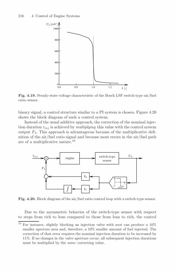
One straightforward approach to realize an air/fuel ratio feedback controlsystem is to use a single switch-type air/fuel ratio sensor upstream of theTWC. The voltage function of a typical switch-type sensor is depicted in Fig.4.19.

Typically, the sensor output is converted to a binary signal, lean for sensorvoltages Uλ smaller than 450 mV , rich for Uλ greater than 450 mV . Using this


Fig. 4.19. Steady-state voltage characteristic of the Bosch LSF switch-type air/fuelratio sensor.

binary signal, a control structure similar to a PI system is chosen. Figure 4.20shows the block diagram of such a control system.

Instead of the usual additive approach, the correction of the nominal injec-tion duration τinj is achieved by multiplying this value with the control systemoutput Fλ. This approach is advantageous because of the multiplicative defi-nition of the air/fuel ratio signal and because most errors in the air/fuel pathare of a multiplicative nature.10

Fig. 4.20. Block diagram of the air/fuel ratio control loop with a switch-type sensor.

Due to the asymmetric behavior of the switch-type sensor with respectto steps from rich to lean compared to those from lean to rich, the control

10 For instance, slightly blocking an injection valve with soot can produce a 10%smaller aperture area and, therefore, a 10% smaller amount of fuel injected. Thecorrection of that error requires the nominal injection duration to be increased by11%. If no changes in the valve aperture occur, all subsequent injection durationsmust be multiplied by the same correcting value.


system shown in Fig. 4.20 produces a bias of the mean value of the air/fuelratio toward lean conditions. To compensate this bias and to achieve a shiftof the mean air/fuel ratio to slightly richer conditions,11 the switch from richto lean is delayed by a time interval tv.

Fig. 4.21. Simulated steady-state behavior of a switch-type control system.

Figure 4.21 shows a simulation of the resulting trajectories for λ and forthe control input Fλ. The fuel path of the engine is modeled as a first-orderlag with a time delay. The dynamics of the switch-type sensor are neglected inthat simulation. This figure also shows the mean value λ of λ that is obtainedby averaging λ using a moving window whose size is compatible with theoxygen storage capacity of the TWC.

In summary, this type of controller has three parameters {kp, ki, tv} thatmust be tuned for every operating point. Since these parameters must be ex-perimentally identified, the parametrization becomes rather time consuming.

The above approach works well as long as the emission levels that have tobe attained are not too demanding. Note that with this control structure, theTWC is operated in an open-loop approach, i.e., its dynamics are not takeninto account.

4.3.3 Feedback Control: H∞

The rather complex dynamic behavior of a TWC has been described inSect. 2.8.3. It is advantageous to include these storage effects in the develop-ment of the fueling control system. In particular, the excursions of the air/fuelratio in one direction must be compensated with equivalent corrections in theother.

11 As discussed in Sect. 2.8.3, the optimal catalytic converter efficiency is achievedfor λ = 0.99 . . . 1.00.


The block diagram of the plant model used to develop the feedbackair/fuel-ratio control-system is depicted in Fig. 4.22. Only the fuel path fromthe injector valves to the air/fuel ratio sensor is considered. The air path isnot included, and all influences of that component are treated as disturbances.

The sensor, which is placed immediately upstream of the TWC, is assumedto be a wide-range sensor, giving not only lean-rich binary information on theair/fuel ratio, but also quantitative values. This sensor is used to form a first,fast air/fuel ratio control loop. In a second stage, an additional air/fuel ratiosensor downstream of the TWC is used to close an outer, slower control loop.This loop takes the oxygen storage capacity of the TWC into account andcompensates for sensor drifts in the inner loop.

Fig. 4.22. Block diagram of the fuel path model.

As in the classical approach discussed in the last section, the output of thecontrol system is a multiplicative factor Fλ that corrects the nominal injectionduration. The error signal used as the input to the control system is definedin a multiplicative way as well.

The outputs of the plant are the air/fuel ratio value at the main confluencepoint λuC (upstream of the TWC) and the mass of oxygen stored in theTWC, mO2,C . The system up to the main confluence point has already beenanalyzed in detail in Chapter 3. However, that model is too complicated tobe used in the design of a feedback control system. Therefore, the completeair/fuel ratio path, from the fuel injectors to the air/fuel ratio sensor at themain confluence point, is approximated by a serial connection of a first-orderlag with time constant τ and a time delay δ

(4.21)

In this expression, the error is defined by ∆λuC = λuC −λuCd, where λuCd isthe demanded value for the upstream catalytic converter air/fuel ratio, andthe linearized input is calculated according to ∆Fλ = Fλ − 1.

A typical measured and simulated step response is shown in Fig. 4.23.The engine used in this experiment is a 1.8-liter four-cylinder SI engine. Theapproach presented below is applicable to any port-injected SI engine. In thissection, the numerical and experimental data will better illustrate that theproposed design methodology is always valid for that engine.

The parameters of this model, i.e., the time constant τ of the lag elementand the time delay δ, depend on the operating point of the engine. An on-line identification for these two parameters is possible using the approach


Fig. 4.23. Simulated (dashed) and measured step response of the engine mentionedin the text; operating point 1500 rpm and 0.1 g air per cylinder per cycle (approxi-mately 25% of fullload).

presented in [186]. A complete map of these two parameters can easily beobtained off-line as well. Figure 4.24 shows an example of such maps for thefull load range and the relevant speed range.12

Fig. 4.24. Time delay δ and time constant τ of the fuel path of a 1.8-liter four-cylinder engine for various engine speeds n and air masses in the cylinder m.

The actual design of the feedback controller can be accomplished in manyways. Here, an approach is shown that is based on the H∞ frequency-domainoptimization technique.13 For this control design method, a linear and finitedimensional system description is required. Therefore, the time delay δ mustbe approximated using a Pade allpass element

(4.22)

12 For higher engine speeds, the parameters do not change substantially because thenon-engine speed dependent factors such as air/fuel ratio sensor time constant,etc. become dominant.

13 For a general discussion of this control system design method, the reader is re-ferred to [53] and, for more information about the engineering aspects, [41] and[175] are good sources.


This approach has been found to be the best approximation method inthis context. The order napx of the approximation is chosen as a functionof the time delay. For delays up to 40 ms, a first-order approximation isrecommended, and for every additional 40 ms, one order should be added. Thisresults in a rather precise approximation of the delay, but also in a rather highsystem order. Accordingly, in order to obtain a small-order control system, anorder reduction step will be necessary.

Inclusion of the Oxygen Storage Capacity

Since the three-way catalytic converter is capable of storing oxygen as wellas carbon monoxide, it is not the actual value of the air/fuel ratio that isrelevant for tailpipe emissions. As long as an excess or lack14 of oxygen can becompensated for by the oxygen storage capability of the TWC, no substantialamounts of emissions are expected at the tailpipe. Only if the storage capacityof the TWC is reached, a rise in the concentrations of NOx or CO and HC,respectively, is to be expected. Therefore, as suggested in (2.228) in Sect. 2.8.3,an integrator is added to the system dynamics described above to model thestorage behavior of the TWC

∆mO2,C =1

s· mO2,uC ·∆λuC (4.23)

The variable mO2,uC defines the oxygen mass flow at the same location wherethe upstream wide-range sensor is placed. For the linear control design, a valuefor mO2,uC equal to 1 is assumed, i.e., a normalized system representation isused. In the controller realization, the correct mass flow will be considered.

Fig. 4.25. Block diagram of the closed-loop system model used for the controlsystem synthesis.

Inner Control Loop

The goal of the first controller’s design is to minimize the impact of an air/fuelratio deviation on the oxygen storage level in the TWC. Using a wide-range

14 Missing oxygen describes rich gas mixtures which result in high levels of CO.


sensor, this must be achieved by measuring only the upstream air/fuel ratio(see Fig. 4.25).

The transfer function from the disturbance d to the oxygen mass ∆mO2,C

stored in the TWC is given by 4.24

GCd(s) =∆mO2,C

d=

1

s· 1

1 + P (s) · C(s)(4.24)

where P (s) has been defined in (4.21) and (4.22) and C(s) is the controllerdesigned below.

Fig. 4.26. Block diagram of the augmented control system used in the H∞ design,where w is the generalized disturbance input and z is the generalized output whosemagnitude has to be minimized.

For the design of an H∞ control system, the plant must be augmented byappropriate weighting functions. The block diagram of the resulting closed-loop system is shown in Fig. 4.26. The associated closed-loop transfer functionTzw has the form

If a stabilizing controller exists that satisfies the conditions ||Tzw||∞ < 1,15

the following two inequalities for the disturbance transfer function GCd andfor the complementary sensitivity Te will be satisfied

|GCd(jω)| < |W−1e (jω)|

|Te(jω)| < |W−1y (jω)|

∀ ω (4.26)

The dynamic weight We(s) thus serves as an upper bound for the mag-nitude of the disturbance transfer function GCd. A possible choice for We(s)is

15 See (A.47) in the Appendix A for a definition of the H∞ norm.


We(s) =1

dmax· s+ ωc

s(4.27)

The corresponding magnitude plot is shown in Fig. 4.27. This diagram alsoillustrates the influence of the two design parameters dmax and ωc on thedisturbance transfer function GCd(s). The parameter dmax limits the maxi-mum value of |GCd(jω)|. At low frequencies, the disturbance transfer functionGCd(s) is forced to zero. This is achieved by the integrator element includedin We(s). The frequency at which this reduction starts can be specified by theparameter ωc.

Fig. 4.27. Magnitude plot of W−1e (jω) (solid) and GCd(jω) (dashed).

To avoid an unnecessarily high bandwidth of the control system, the com-plementary sensitivity Te(s) is limited with an appropriate choice of Wy(s)

Wy(s) =s

kc · ωc(4.28)

where kc ≈ 10 is recommended. An example of the magnitude of the weightingfunction Wy(s) is shown in Fig. 4.28.

The plant parameters τ and δ vary over quite a large range. For the engineexample used in this section, the following range must be considered

δ ∈ [0.02 , 1.0] s τ ∈ [0.01 , 0.5] s

Since the first-order lag in the plant (4.21) can always be compensated, ithas no influence on the weighting functions. The time delay cannot be com-pensated, and the performance specification in the weighting matrices must beadjusted to the varying operating points and, hence, to varying delays. In otherwords, for larger time delays it is mandatory that the demanded bandwidthof the control system is reduced. This leads to the following parametrizationof the design parameters


Fig. 4.28. Magnitude of W−1y (jω) (solid) and Te(jω) (dashed); parameter kc = 13.

dmax = fdmax· δ, ωc =

fωc

δ(4.29)

This choice of the design parameters, which has been found empirically, re-sults in an almost identical Nyquist diagram for all GCd and, thus, in thesame robustness properties over the whole operating range of the engine. Theparameters fdmax

and fωc, which are the same for all operating points, allow

a shaping of the Nyquist curve. The following values have been found to be agood choice for the engine discussed in this section

fdmax= 1.9, fωc

= 0.22 (4.30)

Since the phase shift induced by the time delay cannot be avoided, arobust stabilizing controller must place a significant amount of actuator energy(high loop gain) at frequencies at the opposite of the Nyquist point −1. Thesolution C(s) to the H∞ problem formulated above produces one or severalcharacteristic “bubbles” in the Nyquist diagram of the loop transfer function

L(s) =−1

s · τ + 1· e−s·δ · C(s) (4.31)

in the right half plane, as shown in Fig. 4.29.Assuming that the error in the estimation of the time delay δ is small, this

relatively high gain at frequencies higher than the crossover frequency causesa differential behavior of the loop that adds beneficial damping to the controlsystem. Notice, though, that an error in the identified time delay results in anadditional, usually detrimental phase shift of the Nyquist curve. Accordingly,using more than one “bubble” is only possible with a very accurate systemmodel at hand.

The “one-bubble” form can always be realized with a fourth-order con-troller (the “bubble” requires a complex conjugate pair of poles). If a “no-bubble” form is chosen, then the minimal order of the controller is two, withboth poles at zero in order avoid a steady-state error in ∆mO2,C .


Fig. 4.29. Nyquist plot of the open-loop gain L(jω).

For a disturbance step of 10%, the control system designed in this sectionyields the response depicted in Fig. 4.30. The effect of varying dmax andωc on the resulting trajectories is indicated in the same figure. Decreasingdmax results primarily in a faster descent of the air/fuel ratio back to thestoichiometric value, and thus in a smaller peak of the oxygen to be stored inthe TWC. Increasing ωc results in a faster descent of the total oxygen stored inthe TWC to its reference value. Assuming a constant air mass flow, the returnof the stored oxygen mass to its nominal value obviously can only be achievedif ∆λuC does not return directly to zero but overshoots or undershoots torealize the necessary compensation effects.

Fig. 4.30. Response of the closed-loop system to a step of 10% in the disturbanced(t).


Realization Aspects

As mentioned above, with increasing delay times, the Pade approximation ofthe delay element causes an increase of the model order of the plant and,hence, of the control system. However, a fourth-order controller is sufficientto realize the specific form proposed in the last section. Therefore, an order-reduction step is usually added after the full-order control system has beensynthesized. Any of the well-known order-reduction techniques can be applied.More details of that aspect can be found in [175].

Several state-space forms can be chosen to realize the fourth-order con-troller. Because of the order reduction, the states of the control system aredifferent in each operating point and do not allow any direct physical in-terpretation. Since the control system designed in the last section must begain-scheduled, a fixed, and preferably physically motivated, structure mustbe found. This structure must incorporate the minimum number of param-eters.16 Moreover, the chosen approach must minimize the sensitivity of thecontrol system to parameter errors which may arise due to the gain scheduling.This can be achieved by choosing a structure that utilizes as many parallelelements as possible. For the “one-bubble” solution, the following form is rec-ommended

C(s) = c1 + c2 ·1

s+ c3 ·

1

s2+ c4 ·

s · (c7 · s+ 1)

c25 · s2 + 2 · c6 · c5 · s+ 1(4.32)

The coefficients c1 to c7 are functions of the time delay, of the time constant,or of the operating point defined by engine speed and load. For each operat-ing point, these coefficients are obtained from the result C(s) of the originalcontrol system design by comparing powers of the independent variable s.

Outer Control Loop

The above control system design does not consider the drift of the sensorin front of the catalyst nor the dynamics of the TWC. In fact, this devicehas its own dynamic effects, the most important being oxygen storage. Inthis section the previously designed control system is extended to compensatefor sensor drifts and to consider these dynamic effects as well. This will beachieved by using the information collected by an additional air/fuel ratiosensor downstream of the TWC.

For a realistic physical model of the storage behavior, the varying mass flowthrough the TWC must be taken into account. This is done by multiplyingthe air/fuel ratio deviation ∆λuC with the air mass flow mO2,uC before it isintegrated. The output of the integrator is again divided by the same mass

16 For a “one-bubble” solution, the number is seven. A general fourth-order con-troller has nine parameters, but since in this case two poles are forced to zero,two parameters are structurally fixed.


flow, yielding the structure shown in Fig. 4.31. Using this approach, a correctoxygen balance is obtained without changing the input-output behavior ata fixed operating point. An alternative but equivalent formulation of thiscomponent is possible using the concept of relative oxygen level introduced in(2.228).

The limits 0 and CO2,C of the oxygen storage capacity of the TWC mustbe modeled as well. To estimate CO2,C , dedicated experiments similar to thosewhose results are shown in Fig. 2.68 must be carried out. Since the storagecapacity decreases with time, an on-line identification, as proposed in [185],is necessary.

With ageing of the upstream wide-range air/fuel ratio sensor, a slowly in-creasing offset of its output signal is observed. This offset and the errors in theobserved amount of oxygen must be corrected with an external control loopthat utilizes the downstream air/fuel ratio sensor as the main input signal.Both wide-range and switch-type sensors are used for that purpose. Com-pared to the wide-range sensor, the switch-type sensor, in addition to beingrelatively cheap, has the advantage of offering higher precision in detectingstoichiometric air/fuel ratios.

In both approaches, the outer control loop is chosen to be a relatively“slow” PI controller. The signal from the downstream air/fuel ratio sensor isused to infer the actual oxygen storage levelmO2,C . This estimation problem isnot easy and its solution is the topic of ongoing research. The main difficultyis that as long as the TWC does not reach its storage capacity limits, thedownstream air/fuel ratio sensor will not detect any substantial changes inthe air/fuel ratio in the exhaust gases. Using a switch-type sensor, whose highsensitivity around stoichiometric air/fuel ratios is welcome in this context, anapproximation of the oxygen content is obtained as follows

mO2,C ≈ CO2,C ·

1 if Uλ ≤ 0.2 V

1 − (Uλ − 0.2)/0.5 if 0.2 V < Uλ ≤ 0.7 V

0 if Uλ > 0.7 V

(4.33)

The difference between this measured oxygen level mO2C and the observedlevel mO2,C is the input to a PI controller that produces a correction signalfor the oxygen storage observer. This somewhat indirect approach is chosenbecause of uncertainty with respect to the true oxygen storage dynamics, asmentioned.

The estimated value mO2,C of oxygen stored in the TWC is compared tothe corresponding desired17 value mO2,C , and the resulting difference is usedas input signal to the “buffer control” component. The resulting control systemstructure is shown in Fig. 4.31. Note that the gain c3, which depends on theengine’s operating point, must be placed in front of the second (rightmost)

17 A value of mO2,C = 0.6 · CO2,C is recommended.


integrator to avoid an excitation of the controller because of varying operatingpoints. If no controller action is required, the input to the integrator will bezero. Therefore, varying the gain c3 does not affect the output of the controllerif it is placed before the integrator.

Fig. 4.31. Block diagram of the complete air/fuel ratio control system.

Experimental Results

To demonstrate the benefits of the proposed control system, especially ofits capability to automatically adapt the bandwidth of the closed loop tochanging operating points, the results of simulations and measurements attwo operating points are shown below. The precise definition of the two casesanalyzed is given in Table 4.1. The first operating point (OP 1) was alsoused for the simulations shown above. Note that in OP 1, the time delay δcorresponds to almost 14 segments. This large delay substantially limits theachievable bandwidth of the feedback control system.

Figure 4.32 shows the response of the upstream lambda buffer controlsystem for a disturbance18 step at dF as defined in Fig. 4.25.

Because of the parametrization of the control system parameters proposedabove, the two system responses have similar properties. However, because the

18 The signal dF is the more realistic choice as a disturbance source than the signald. The latter represents the worst case situation because it acts immediately onthe controller and is preferable for the design of the control system.


Table 4.1. Operating points chosen in the experiments.

operating point OP 1 OP 2

engine speed n [rpm] 1500.0 1500.0cylinder air-mass mair,cyl. [g] 0.1 0.3engine torque Te [Nm] 18.0 80.0time delay δ [s] 0.27 0.116time constant τ [s] 0.192 0.146segment time τseg [s] 0.02 0.02cycle time τcycle [s] 0.08 0.08

Fig. 4.32. Response of the upstream lambda buffer control to a -20% step (left)and a +20% step (right) in the disturbance dF .

time delays in OP 1 and OP 2 are different, the bandwidths of the controlsystems vary accordingly.19 The maximum deviation of the air/fuel ratio inOP 1 is slightly larger than in OP 2 because of the larger time delay. Also,the maximum value of the integrated λ error is larger in OP 1 than in OP 2.Nevertheless, because of the substantially smaller air mass flow, the error instored oxygen is not as large.

The variations of the oxygen storage level in the TWC are used to assessthe performance of the “buffer control system” to adapt to changing operatingconditions. Since the oxygen storage level cannot be measured directly, theoutput of the switch-type air/fuel ratio sensor downstream of the TWC istaken as a measure of that quantity. It is reasonable to assume that if theoxygen storage level of the TWC remains constant, the composition of theexhaust gas remains nearly constant as well. Accordingly, the output voltageof the downstream sensor remains constant, too.

The transient test used to assess the performance of the proposed controlapproach consists in rapidly (in approximately 100 ms) opening the throttleplate from 9 ◦ to 24 ◦. In steady-state, the mass of air entering the cylinder ineach cycle due to that change is increased by a factor of three. The delayedincrease in air mass visible in Fig. 4.33 is a consequence of the manifold

19 Notice that a scaling of the time t, according to the ratio of the delays, producesalmost congruent curves.


Fig. 4.33. Response of the complete control system to a step in the throttle com-mand corresponding to a change from OP 1 to OP 2. The variable Uλ2PdC

denotesthe voltage of the switch-type air/fuel ratio sensor downstream of the catalytic con-verter.

dynamics. Moreover, to amplify the errors in the air/fuel ratio, the feedforwardcontrol action for the fuel injection has been reduced in these experiments.

The results of this test are shown in Fig. 4.33. In spite of the large increasein air mass and in spite of the reduced action of the feedforward control system,the downstream sensor output remains almost unchanged. This result can betaken as an indication for a constant oxygen storage in the TWC in thesteady-state conditions.

4.3.4 Feedback Control: Internal-Model Control

Ideally, the efficiency of modern pollution abatement systems should be main-tained over the whole lifetime of its components. To that end, it is indispens-able to account for the ageing of the components involved. Specifically, theTWC and the wide-range λ sensor may undergo considerable changes in theirdynamical properties during their lifetime. In section 2.8 it is shown that fora tight control of the oxygen level in the TWC with consideration of ageingeffects, a more detailed, control-oriented model than the one presented in 4.23may be necessary. In the preceding section the TWC model was included inthe design process of the air/fuel ratio controller. However, with a more de-


tailed model this neither seems to be beneficial nor tractable in practice. Asdepicted in Fig. 4.34, the controller for the oxygen level, based on the detailedmodel and the air/fuel ratio controller, are therefore structurally arranged ina cascaded control scheme, where the air/fuel ratio controller is in the innerand the oxygen level controller is in the outer loop, respectively. In this setup

6-

tinj

- - -?fuel path-

λ sensor

λuC× TWC -λdC

λ sensorwide-range switch-type

Fλ---

6- balancing

controller

λ

controller

Fig. 4.34. Schematic air/fuel ratio control system.

the air/fuel ratio controller can be designed independently of the controllerfor the oxygen level, and the output of the level controller acts as the referencesignal for the air/fuel ratio control system in the inner loop. As a consequence,the new air/fuel ratio controller needs to be optimized with respect to bothdisturbance rejection and reference tracking.

To account for variations in the wide-range sensor dynamics due to ageingof the sensor cell and clogging of the vent holes, an adaptive extension of theair/fuel ratio controller will be inevitable to meet future emission regulations.It is therefore important to choose a control structure that offers the premisesfor such extensions.

For processes where an input-output model is available, specifically forstable SISO processes, the internal model control (IMC) structure depictedin Fig. 4.35 offers an intuitive control design procedure that is compatiblewith the above-mentioned requirements of the air/fuel ratio control system.The separation of a controller into an internal model P (s) and an internal

6-

r e u yd

6P-

�

- - - -?Q

Py

-

Fig. 4.35. IMC system.

controller Q(s) also allows a natural handling of processes incorporating atime delay. The transfer function of the control system in Fig. 4.35 can bewritten as


T (s) =P (s)Q(s)

1 + (P (s) − P (s))Q(s)(4.34)

In the case of a perfect model, i.e., P (s) = P (s) the transfer function T (s)becomes

T (s) = P (s)Q(s) (4.35)

thus, for open-loop stable plants the control system in Fig. 4.35 is stable forall stable transfer functions Q(s). Furthermore, in the case of a perfect model,the signal y cancels the feedback signal y, i.e., the feedback path only is “acti-vated” in the presence of external disturbances and modeling errors, whereasotherwise the internal controller Q(s) acts as a pure feedforward controller.This property reflects the very nature of the interaction of feedforward andfeedback control.

The design of the internal controller Q(s) is usually done in two steps:20

in a first step a nominal controller Q(s) is designed that minimizes the controlerror e for a representative disturbance d

Q = arg minQ

‖e‖2 (4.36)

subject to the constraints of stability and causality of Q. With (4.35) theproblem (4.36) can be rewritten as

Q = arg minQ

‖(PQ− 1) ·D‖2 (4.37)

where D is the Laplace transform of the signal d. Obviously, for minimum-phase systems the solution of (4.37) is21

Q = P−1 (4.38)

In the second step an IMC filter F is added to the nominal controller Q

Q = Q · F (4.39)

to account for modeling errors and to obtain a realizable transfer function Q.Given the relative uncertainty bound W2 of the model P

∣∣∣∣∣P (jω) − P (jω)

P (jω)

∣∣∣∣∣ ≤W2(ω), ∀ω, (4.40)

the robust Nyquist theorem states that the closed control loop is asymptoti-cally stable if the inequality

20 For detailed information about the design of internal model controllers the readeris referred to [145].

21 For non-minimum-phase systems and systems with a time delay the optimal so-lution of (4.37) is also dependent on the shape of the disturbance d.


|T (jω)W2(ω)| < 1 (4.41)

holds. With (4.35) and (4.39) the inequality (4.41) can be written as

|P (jω)Q(jω)F (jω)W2(ω)| < 1 (4.42)

and thus the IMC filter F can be used to shape the complementary sensitivityT to obtain a robustly stable control system. This step is often referred to as“detuning” of the nominal controller Q.

Given the model of the fuel path in (4.21) and the assumption that themain disturbances acting on the control system are step-shaped22, the nominalair/fuel ratio controller Q is obtained by inverting the model of the fuel pathwithout the delay time

Q(s) =τs+ 1

−1. (4.43)

The delay time δ of the fuel path provides an upper bound for the achievablebandwidth of the control system. To account for this upper bound, the IMCfilter F is chosen as

F (s) =1

δσs+ 1

, (4.44)

where σ is a tuning parameter for the bandwidth of the control system. Theresulting internal controller can then be written as

Q(s) = − τs+ 1δσ s+ 1

. (4.45)

With (4.35) the nominal complementary sensitivity T (s) can now be writtenas

T (s) =1

δσ s+ 1

e−sδ. (4.46)

The transfer function of the nominal open loop gain L(s) can be written as

L(s) =e−δs

δσ s+ 1 − e−sδ

. (4.47)

Given the facts that L(s) is independent of the time constant τ and that thedelay time δ only appears as a factor for the Laplace variable s, the shapeof the Nyquist curves shown in Fig. 4.36 is dependent only on the parameterσ and not on the parameters τ and δ. This fact can be interpreted as aconstant robustness of the control system for all operating points. As shownin Fig. 4.36, large values of the bandwidth parameter σ lead to bubbles in the

22 This is a valid assumption since the feedback controller is primarily designedto compensate for the static errors of the feedforward controller, whereas thebandwidth of transient errors due to the feedforward control action is much higherthan the bandwidth of the feedback control system.


real

imag

σ = 0.7

real

σ = 1

real

σ = 2

-1 0 1-1 0 1-1 0 1-2

-1.5

-1

-0.5

0

0.5

1

Fig. 4.36. Nyquist diagram of the nominal open air/fuel ratio IMC loop, for differentvalues of σ. The dashed line indicates the Nyquist curve for σ → ∞. The shape ofthe Nyquist curve is independent of the plant parameters.

right half plane of the Nyquist diagram. This is due to the increased derivativecontrol action that is necessary to achieve the demanded bandwidth. Asidefrom the common issues with regard to amplification of measurement noise,the bubbles can lead to undesired control actions at high frequencies. Morespecifically, in air/fuel ratio control too high a value of σ may lead to controlaction due to an imbalanced air/fuel ratio in the single cylinders. This isundesirable since the model in (4.21) does not account for these effects andthus the imbalance of the cylinders may even increase due to the controlaction. Various experiments have shown that a value of σ = 0.7 results in agood trade-off between performance and robustness. However, when a higherbandwidth is required, the magnitude of the loop gain at high frequencies maybe reduced by adding a further lowpass filter to the IMC filter.

Implementation of the IMC

Implementation of the Delay Time

The delay time in the internal model of an IMC is a critical element for itsimplementation in software. It is yet unclear how to efficiently implement thedelay time block in the general case with fast variations in the ratio of thedelay- and the sampling time. However, this issue can often be circumventedby a proper choice of the basis for the sampling time and by a physicallymotivated implementation of the delay time. Specifically, for the air/fuel ratiocontroller the sampling time ts is chosen to be equal to the segment timetseg of the engine. Figure 4.37 indicates that in the main operating rangethe variations of the ratio between the delay time δ of the fuel path and thesegment time tseg of the engine are small. When the control system is sampledat the segment frequency, the delay time can be implemented as a memoryblock with a constant part and variable part, where the constant part accountsfor the delay time due to the engine cycle and the variable part accounts for the


6

7

7

8

8

89

9

9

9

1010

10

1111

11

11

n [rpm]

rela

tive

load

[%]

1000 1500 2000 2500 3000 3500 4000 4500 5000

20

25

30

35

40

45

50

55

60

65

70

Fig. 4.37. Ratio between delay time δ and the segment time tseg over the wholeoperating range of an engine with 5 cylinders. The gray line represents the trajectoryduring the FTP-75 cycle.

gas transport in the exhaust manifold. In Fig. 4.38 a possible implementationstrategy of the delay time is depicted schematically. The estimated value ofthe delay time δ usually is obtained from an engine map as a function of therelative load and the engine speed.23 However, the physical delay due to thegas transport in the exhaust manifold is a function of the thermodynamicproperties of the exhaust gas, i.e., the estimated and the physical transportdelays are “separated” by about one engine cycle. As shown in Fig. 4.38, toovercome this separation the variable part of the memory stack is placed infront of the constant part and the input to the memory is moved in accordancewith the variable delay time. When the memory input is moved to the right,i.e., the variable delay time is reduced, all values in the cells on the left-handside of the memory input are dropped and the value in the active input cell isoverwritten by the new value of yτ . This can be interpreted physically as theexhaust gas that passes the λ sensor between two sampling events. When thememory input is moved to the left, i.e., the variable delay time is increased,empty memory cells are generated. A physically correct filling of the emptycells would require an inter-sampling of the values of the model output yτ ,e.g. if the memory size is increased by one cell, the (new) first cell is filled

23 In this context the engine speed is not relevant since it is shown in subsection2.5.2 that the dynamics of the engine speed are much slower than those of theintake manifold.


-�-�Engine cycleGas transport

tseg tseg

y

?

6yτ

-�

−1

τs+ 1-u

-�round(δ/ts)

Fig. 4.38. Implementation of the delay time.

with the actual value of yτ at time tk and the value of yτ at time tk−1 of thesecond cell is shifted to the third cell at the same time, i.e., the second cellbecomes empty and should thus be filled with the value of yτ at time tk−0.5.As a consequence of this process, assuming that the memory size is maximallyincreased by one per sample, a correct treatment of an increase in the memorysize would require that the signal yτ is computed at twice the actual samplingfrequency. This assumption is justified by the numbers shown in Table 4.2which show the distribution of the occurrence of changes in the ratio of thedelay time and the segment time during an FTP cycle.

Table 4.2. Distribution of changes in memory size per sample (segment time) duringthe first 1200 s of the FTP-75 cycle

∆ memory size -2 -1 0 1

occurrence 0.02% 2.42% 96.28% 1.28%

When the given resources prohibit the use of a memory stack, the delaytime could also be implemented as a finite dimensional approximation, e.g.a Pade element as shown in (4.22) and (B.18). However, in this case theapproximation would contribute to the model error, which may have to beconsidered in the design of the IMC filter.

Static Errors

Static deviations from the stoichiometric air/fuel ratio have a detrimentaleffect on the performance of the TWC. It is therefore important for the con-troller to have a high gain at low frequencies. If the IMC has been designedaccording to the procedure outlined in the previous section, i.e., the staticgains of the internal controller Q and the internal model P are reciprocal, itholds that


limω→0

∣∣∣∣∣Q(jω)

1 − P (jω)Q(jω)

∣∣∣∣∣ =1/k

1 − k · 1/k = ∞. (4.48)

This results in a perfect cancellation of static disturbances. However, an ECUoften allows computations at a relatively low precision only. This may leadto different static gains in the feedforward and in the feedback path, whichresults in a finite static gain of the controller

limω→0

∣∣∣∣∣Q(jω)

1 − P (jω)Q(jω)

∣∣∣∣∣ =1/k

1 − (k + ∂k) · 1/k =1

∂k, (4.49)

and thus a static control error of ∂k · 100%. It is thus important that thecomputations are optimized with respect to the precision of the static gainsof the internal model P and the internal controller Q. A different approachto reduce static errors due to quantization is to implement the IMC in theSmith predictor structure as depicted in Fig. 4.40. The internal controller CIof the Smith predictor can be written as

CI =Q

1 −QP. (4.50)

For the air/fuel ratio controller designed with (4.45), the internal controllerCI can be derived as

CI =Q

1 − F= −στ

δ

(1 +

1

τs

)(4.51)

which is a PI controller. The computations that are performed in the twointernal model feedback paths of the Smith predictor shown in Fig. 4.40 onlydiffer by a shift register due to the delay time. Thus, under static conditions,the error eδ is zero, irrespective of the computational precision, whereas theSmith predictor is reduced to the internal controller CI which contains apure integrator that can be optimized for the static precision of the controlsystem. Figure 4.39 depicts the static error of the control system with anIMC structure and a Smith predictor structure, respectively, when a fixed-point arithmetic with a word length of 16 and a precision of 12 bits is used.The static error is evaluated for 1000 random samples of the two parametersτ and δ. The samples of both parameters are uniformly distributed, rangingfrom 0.07 s to 0.32 s, with the sampling time chosen to be 10 ms. The Smithpredictor results in a considerably smaller static error due to its structuralproperties mentioned. However, the precision of both controller structures canbe improved by simple measures such as an individual adjustment of the fixed-point resolution for all variables of the controller and a systematic reorderingof the calculation steps. In the Smith predictor structure only the computationof the integrator in the internal controller CI needs to be optimized for staticprecision, whereas in the IMC structure the computation in both the internalcontroller Q and the internal model P needs to be optimized.


sam

ple

s[-]

λ error [%]

IMC

Smith predictor

-5 -4.5 -4 -3.5 -3 -2.5 -2 -1.5 -1 -0.5 00

50

100

150

200

250

300

350

400

450

Fig. 4.39. Comparison of the static control error of the two control structures forrandom samples of the plant parameters τ and δ.

Integrator Windup

In classical PID control loops, actuator saturation can lead to a windup ofthe open integrator in the controller. This problem is typically tackled byextending the control structure with some sort of heuristic integrator windupprotection (see A.7.2 for some general remarks). In the IMC structure, usuallyno apparent open integrator is present. However, as shown in the precedingsection, the integrator action evolves from the interplay of the internal modeland the internal controller. This implies that a controller windup can also beobserved with an IMC system when no proper measures are taken in the caseof actuator saturation. Fortunately, the IMC structure allows a systematic

r e u

� �

- -CI

P

�

6

-

6

6

---

P · e−sδ

eδ

�

- yd

- -?P · e−sδ

Q

Fig. 4.40. Structure of the Smith predictor and the IMC (dashed) with anti windupmeasure.


treatment of actuator saturation and other input nonlinearities. To that end,a model of the nonlinearity must be included at the input of the internal model.The same strategy equivalently translates to the Smith predictor structure asdepicted in Fig 4.40, where a model of the saturation is added at the input(and only there) of the internal model containing the delay. Note that, incontrast to standard PI controllers, the integrator in the internal controllerCI does not need any special treatment in the case of actuator saturations.Figure 4.41 shows the simulated system response of the air/fuel ratio IMCwith actuator saturation for a disturbance pulse with an amplitude that islarger than the saturation limit. As expected, the control system with theanti windup measure has a smaller transient after the saturation period.

Experiments

Figure 4.42 depicts the response of the IMC system for steps in the nominalinjection time at two different operating points. At both operating points theλ signal comprises variations of the air/fuel ratio at a relatively low frequency.These variations mainly occur at operating points where the throttle is almostclosed and thus the air flow past the throttle is very sensitive with respect tothe throttle position. However, these air/fuel ratio variations usually consti-tute no problem for the pollution abatement system and thus, need not be

[-]

time [s]

ywindup

yantiwindup

d

uwindup

uantiwindup

0 0.5 1 1.5 2 2.5 3 3.5 4 4.5 5-0.8

-0.7

-0.6

-0.5

-0.4

-0.3

-0.2

-0.1

0

0.1

0.2

0.3

Fig. 4.41. Simulated system response for a disturbance pulse at the input of aplant with actuator saturation of ±0.25. The black curves are with and the grayones without anti windup measure according to Fig. 4.40. Parameters: τ = 0.15 s,δ = 0.15 s, σ = 1.


damped by the controller. The λ signals in Fig. 4.42 also contain fast vari-ations due to the air/fuel ratio deviations of the individual cylinders. Thesefrequencies must not be damped by the controller, as these effects are notmodeled by 4.21 and thus, cylinder unbalancing could even be increased bythe control action.

PSfrag

∆λ

[-]

∆λ

[-]

time [s]0 1 2 3 4 5 6 7 8

0 1 2 3 4 5 6 7 8

-0.05

0

0.05

-0.05

0

0.05

Fig. 4.42. Simulations (gray) and measurements (black) of the response of the con-trol system with disturbances (dotted) at the input of the plant. Operation points:1500 rpm and relative load of 30%, corresponding to a time constant of τ = 0.14 sand a delay time of δ = 0.13 s (upper plot), and 2250 rpm and relative load of 40%corresponding to a time constant of τ = 0.08 s and a delay time of δ = 0.07 s (lowerplot), both with σ = 0.7.

4.3.5 Multivariable Control of Air/Fuel Ratio and Engine Speed

The time delays in the various signal paths are largest when the engine isidling. Therefore, instead of having two parallel control loops that can disturbeach other, in this situation it is advantageous to combine the air/fuel ratioand the idle-speed control problems into one single MIMO control system.The classical SISO idle speed control problem is analyzed in more detail inAppendix B. In the case studied here, taken from [175], the correct handlingof the multivariable nature of the combined control problem is emphasized.

The block diagram of the control system that is analyzed in this sectionis shown in Fig. 4.43. The reference values for the air/fuel ratio as well as


Fig. 4.43. Block diagram of the combined air/fuel ratio and idle speed controlsystem.

for the engine speed are obtained from the accelerator pedal signal by anappropriate signal interpretation module. The sensor signals that are used bythe control system are the measured air/fuel ratio, the engine speed, and theair mass flow into the intake manifold. Although there is no reference valuefor the air mass flow signal, including it in the loop improves the quality ofthe observer that is a part of the MIMO control system. Because of large timedelays, the spark advance uζ must be used in addition to the throttle and thefuel command, as a third control channel. A basic control system that takescare of the steady-state control actions for ignition and fuel is implementedin a first step (block “static maps” in Fig. 4.43). That step, which optimizesthe fuel consumption and minimizes the engine-out pollutant emissions, is notdiscussed here.

A naturally-aspirated and port-injected SI engine without external EGRis considered. The engine from which the experimental data shown belowhas been obtained has four cylinders and a displaced volume of 1.8 liter.It is mounted on a dynamic test bench that can apply load steps on theengine with a bandwidth of approximately 5 Hz. The focus of the followinganalysis is on the dynamic behavior of the engine system. Changes in the loadtorque Tl are assumed to be the main disturbances. A simple model of thecorresponding engine dynamics, which will be used for the subsequent designof the control system, is shown in Fig. 4.44. Compared to the block diagramshown in Fig. 2.5, it explicitly includes the four dominant time delays and thestatic control maps mentioned above.

The static engine control algorithms run on a separate process controller.Only static maps for the fueling command and the spark advance are applied.The fueling command relies on the measurements of the air mass flow into


Fig. 4.44. Block diagram of the “plant” component of Fig. 4.43.

the intake manifold. Thus, the controller to be designed also must take intoaccount errors made by this feedforward component of the fuel control system.In steady-state operation, the throttle valve correction signal must compensateall load disturbances, whereas the fueling correction signal eliminates errors inthe air/fuel ratio. The spark advance correction may only be used in transientsand must go back to zero under steady-state operating conditions.

For small variations of the input signal, the dynamics of the electronicthrottle valve are assumed to be well approximated by a first-order lag ele-ment. For large steps, the current saturation of the DC motor becomes active,making the air flow actuator strongly nonlinear. The wall-wetting dynamicsare assumed to be of first order, as described in Sect. 2.4.2. The air/fuel ratiois measured with a wide range sensor. The sensor voltage is linearized and thesensor dynamics are approximated by a first-order lag element with a timeconstant of 20 ms. The remaining two integrators describe the emptying andfilling dynamic of the intake manifold and the rotational inertia of the engine.Figure 4.45 shows the block diagram of the resulting linear engine model.

The control system to be designed must fulfill the following requirements:

• No steady-state error in engine speed and air/fuel ratio are permitted forall load disturbances in the range [0, 20] Nm.

• The controller must be robust to modeling errors, i.e., the minimum returndifference of the open loop may not be smaller than 0.5.

• The spark advance control channel may only be used during the transients.• The controller must be operated in the crank-angle domain and discretized

on a segment-to-segment basis.


Fig. 4.45. Detailed block diagram of the linear engine model (including the delays).

Table 4.3 provides overview of the explicit numerical values of all constantsused in Fig. 4.45. These parameters are valid for a four-cylinder 1.8-liter engineat idle conditions.

Table 4.3. Parameters of the linearized engine model shown in Fig. 4.45 at idleconditions.

param. value param. value

k2 40 [rad/s] k13 0.00116 [1/rpm]k3 43.6 [g/min/◦] k14 0.000402 [g/min/rpm/rpm]k4 77.5 [g/min/bar] k15 2.90 [rev/g]k5 0.00386 [bar·min/s/g] k17 5.7 [rad/s]k6 686 [g/min/bar] k18 7.76 [Nm/bar]k7 0.422 [g/rev] k19 0.3 [-]k8 114 [Nm·rev/g] k20 15 [rad/s]k9 -16.3 [Nm] τUinj→TC 0.14 [s]k10 0.0984 [Nm/◦CA] τUign→TC 0.07 [s]k11 0.00358 [Nm/rpm] τIC→TC 0.07 [s]k12 63.7 [rpm/Nm/s] τTC→λmeas 0.385 [s]

The control system is designed using a model-based approach by apply-ing the H∞ frequency-domain optimization method. The block diagram of thelinearized engine model used in that synthesis procedure is shown in Fig. 4.45.The resulting observer-based controller has 13 state variables. Five state vari-ables are necessary to observe the relevant level variables in the engine system.Two additional state variables are used to force the steady-state errors of the


air/fuel ratio λ and of the engine speed ωe to zero. The remaining six statevariables are used to approximate several delays present in the system. Usingthis rather large number of state variables allows to establish the achievableperformance limits to be established. Of course, in a real application, an or-der reduction step would have to follow in order to obtain a realizable controlsystem.

A comparison between simulation and measurement is shown in Fig. 4.46and Fig. 4.47. Figure 4.46 shows a load step. The offset in spark advance islimited to +5◦ crank angle. An appropriate anti-windup scheme is used.

Fig. 4.46. Control system behavior, load step ± 20 Nm at 1 s and 9 s, respectively.

The tracking behavior is depicted in Fig. 4.47. Since the throttle must beactuated for steps in the demanded engine speed, the air/fuel path is excitedas well. Deviations of up to 7% are observed, nevertheless they are reducedwithin one second to values below 3%. On the other hand, excitation of the


air/fuel ratio demanded result in engine speed deviations of only 20 rpm,which are hardly noticeable.

Fig. 4.47. Control system behavior, steps of the demanded values at 1 s and 9 s;respectively; a) engine speed steps (±200 rpm), b) λ steps (±10%).

Finally, in Fig. 4.48, the performance of the MIMO controller designedabove is compared to the performance of the series-production type controller.This controller uses two parallel SISO control loops for the air/fuel ratioand the engine speed, respectively. Since the speed set point of the series-production type controller is 770 rpm, this value was chosen in all experiments.Moreover, since the series-production type controller was not able to handle adisturbance of 20 Nm, the load step was reduced to 10 Nm in these particularexperiments.

4.4 Control of an SCR System

The purpose of a selective catalytic reduction system was discussed in sec-tion 2.9. The model developed in that section forms the basis for the controlsystem synthesis discussed below. In the case studied here, based on [178],the tailpipe NOx emissions of a heavy-duty Diesel engine (that was certifiedfor the Euro II limits) have been reduced to meet the Euro V emission limits.To achieve this reduction, a minimal NOx reduction rate of 50% is necessary.Since tailpipe emissions of NH3 are highly undesirable, a maximum mean slipof only 10 ppm of ammonia is tolerated.

4.4 Control of an SCR System 245

Fig. 4.48. Measured control system performance, load steps at idle speed: ±10 Nmat 1 s and 9 s, respectively.

The engine that is considered in this section is a 10-liter superchargedheavy-duty, direct-injection, Diesel engine with intercooler. Its rated power is275 kW. The maximum engine speed is 2150 rpm.

The amount of NOx in the exhaust gas and the amount of ammonia in-jected vary strongly as functions of the engine operating point. Changing en-vironmental conditions and the ageing components of the engine system playan important role as well. The dependency of the engine-out emissions uponthe engine’s operating point can be considered by implementing correspond-ing maps and by adding a low-pass filter to account for the thermal dynamics.All other effects (plugging of the injection system, change in ambient condi-tions, ageing) and the unavoidable modeling errors render a feedback controlsystem necessary. Such an approach is only possible if information is availableregarding the NOx concentration in the exhaust upstream and downstream ofthe catalytic converter. The available solid-state NOx sensors (Siemens-NGK“Smart NOx Sensor,” SNS) show significant cross-sensitivities to ammonia.Therefore, close to the optimal dosage, where it is not clear whether excessive

Fig. 4.49. Engine-out NOx emissions in ppm of a 10-liter, heavy-duty Diesel engine.


amounts of NOx or NH3 are present, the sensor signal cannot be interpretedin a straightforward way.

Figure 4.49 shows the map that is used for the calculation of the steady-state engine-outNOx emissions. The output of the steady-state map is filteredwith a lag-lead element with a time constant of 20 s and a feed-through of 0.75.Figure 4.50 shows the measured and estimated engine-out NOx emissions forpart of an ESC test.24

Fig. 4.50. Measured and estimated engine-out NOx emissions for part of an ESCtest. Starting at 400 Nm and 1590 rpm, a step to 1365 Nm and 1900 rpm is per-formed, then a step to 350 Nm, followed by a step to 1020 Nm, and finally a stepto 695 Nm, all at 1900 rpm.

Figure 4.51 shows the relevant variables for a sweep in ammonia dosage.The cross-sensitivity to the ammonia concentration for higher-than-stoichio-metric ammonia dosages is obvious. The ”true”NO concentration is measuredwith a standard emission testing device, whereas the ammonia concentrationis measured with a dedicated instrument.

Due to ammonia storage effects in the catalytic converter, the SNS sensorsignal is substantially less noisy when the value of α/αOD

25 is larger than one.Using this property, an additional periodic modulation of the dosage signalcan be used to separate the α/αOD < 1 portion from the α/αOD > 1 part.In fact, the amplitude reduction caused by the catalytic converter is used todecide in which regime the system is working and, thus, to calculate the outputindicated by SNS,pp that represents an estimation of the NOx concentration.Notice that in the case of excess ammonia this value can be negative.

This interpretation of the NOx sensor signal allows for the implementationof a true SCR feedback control system. Of course, this component has tobe complemented by an appropriate feedforward control scheme in order to

24 The ESC test cycle is the equivalent of an MVEG-95 cycle for heavy-duty Dieselengines.

25 The variable αOD is the optimal dosage ammonia feed ratio, defined as the rationNH3,u

nNOx,uwhere an ammonia slip of 10 ppm is observed.

4.4 Control of an SCR System 247

Fig. 4.51. Output signals of a solid state NOx sensor (SNS), true NO signal (NO),and NH3 concentration in the exhaust gas for a sweep in ammonia dosage. Thepost-processed sensor signal (SNS,pp) is also shown.

achieve the best possible bandwidths. Figure 4.52 shows the block diagram ofthe combined control scheme.

Fig. 4.52. Block diagram of the combined feedforward/feedback SCR control sys-tem.

The main elements of the proposed SCR control system are:

• Engine model: The signals available in the standard ECU (engine speedand load, temperature and pressure in the intercooler, temperature up-stream and downstream of the catalytic converter, etc.) are used to calcu-late an estimate of the engine-out concentration ofNOx and the engine-outmass flow. As indicated, this can be done by using appropriate maps. Thesteady-state NOx engine-out emissions are then filtered with a first-order


lag-lead element with a time constant of 20 s in order to account for thethermal dynamics of the system.

• Dynamic model of the SCR system: The output signals of the engine modeland the measured exhaust gas temperature upstream of the converter sys-tem are the inputs to an observer for the SCR system. The observer usesthe simplified two-cell model described in Sect. 2.9. All states of the modelare calculated, taking into account the actual injected amount of urea so-lution.

• Feedforward control: By inverting (2.248) and (2.249), the demanded valuefor the amount of urea solution injected and the SCR system-out (tailpipe)emissions of NOx can be calculated. In this step, the demanded value forthe tailpipe ammonia slip is chosen to be 10 ppm.

• Feedback control: The demanded amount of injected urea solution is mul-tiplied by the output of the feedback controller. The control error is thedifference between the calculated amount of tailpipe emissions of NOxand the interpreted sensor output. The feedback element is a simple PIcontroller that is designed using classical frequency-domain methods, asexplained in Appendix A. This PI control system may be chosen to berather “slow” because it only has to cope with the disturbances originat-ing from the environment and from ageing components.

• Signal processing: In order to separate theNOx information from the NH3

information in the sensor output signal, the product of the outputs of thefeedback and feedforward control systems is modulated with a periodicsignal with an amplitude of approximately 10%. This filtered output formsthe reference signal for the urea dosage unit. A local dosage control systemguarantees a good agreement of the mass flow of urea injected with thisreference value.

Figure 4.53 shows the performance of the SCR control system for an ESCtest cycle. The experimental verification of this control strategy showed anaverage NOx reduction of almost 90%, while the ammonia slip was kept atan average value of 10 ppm. Note that some ammonia slip is present evenif the exact stoichiometric urea dosage is applied all of the time. Therefore,lower ammonia slips can be achieved only by accepting a deterioration of theefficiency of the NOx reduction. Moreover, the measured value of 10 ppm liesbelow the limit which is considered to be harmful and is below the humanperception limit as well.

A further improvement of the performance of the control system can beachieved by accepting ammonia slips that are proportional to the tailpipeNOxemissions. As before, equations (2.248) and (2.249) can be used for the cal-culation of the demanded amount of urea solution and the estimated tailpipeNOx emissions. The resulting control system structure remains essentially thesame, but when necessary, higher ammonia slips are accepted for the sake ofan improved NOx reduction.

4.5 Engine Thermomanagement 249

Fig. 4.53. Performance of the SCR system during an ESC cycle on a superchargedheavy-duty engine with Vd = 10l. NOx,u and NOx,d are the upstream and down-stream molar flows of NOx, respectively, and NH3,d represents the downstreammolar flow of ammonia.

4.5 Engine Thermomanagement

4.5.1 Introduction

In automotive applications, approximately one third of the fuel energy deliv-ered to the engine must be removed by the cooling system [97]. In high-speedand high-load operating points this amounts to significant amounts of heatflux. Specifically, at high ambient temperatures and low vehicle velocities,large radiators, additional fans, and large thermostats must be used to guar-antee that the cooling system works properly and that the engine does notoverheat. Accordingly, when the engine runs in part-load conditions, which isthe case most of its lifetime, the cooling effect is too large. This leads to lowerfuel economy due to lower engine temperatures and therefore higher frictionlosses. In addition, considerable losses are caused by the mechanically drivenwater pump and by the inefficient thermostat used to control the coolanttemperature.

While the drawbacks of a mechanically coupled water pump are obvious,the drawbacks of the conventional thermostat must be explained in more


detail. As shown in Fig. 2.44, the thermostat is a valve whose position deter-mines the flow distribution between the radiator and its bypass duct. Understationary conditions, the position of the thermostat is defined by the coolanttemperature. The active element of the thermostat (a wax element) has dy-namics that cannot be neglected. The time constant of this element amountsto approximately 30 s. For cold starts at high loads, the engine temperaturemust be kept from overshooting to avoid damage to the cylinder head gasketsand other components. Therefore, the thermostat’s static characteristic mustallow a certain amount of coolant to flow through the radiator, even at rela-tively low temperatures (70◦C). On the other hand, at 90◦C, the thermostatmust be fully open to enable maximum cooling. These requirements lead toa nonlinear static gain function as shown in Fig. 4.54. The thermostat actsas a proportional controller. Since the plant itself does not have any integrat-ing behavior, this simple control system cannot avoid errors in steady-stateconditions. In particular, at higher engine speeds and at lower loads, this tem-perature deviation from the demanded value leads to higher friction losses inthe engine and, thus, higher fuel consumption.

Fig. 4.54. Lift characteristic of a conventional thermostatic valve.

4.5.2 Control Problem Formulation

Modern engine cooling systems include electrically driven water pumps andelectronically controllable bypass valves. The higher cost of these componentsmust be compensated for by improvements in the overall fuel efficiency of thesystem. This requires improved control strategies which are able to operate theengine at part load at higher temperatures, yet still guarantee proper systemcooling at high loads. A detailed mathematical model of such a cooling systemwas developed in Sect. 2.6.5. Here, the design of the corresponding controlsystem is discussed.


The new cooling system offers two independent control inputs. The addi-tional degree of freedom can be used to simultaneously control the temper-atures of the coolant entering and leaving the engine. Similarly to the con-ventional approach, the temperature ϑeo of the coolant leaving the engine isset to a demanded value of ϑeod ≈ 90 ◦C. The temperature ϑei of the coolantentering the engine is controlled using the actual value of ϑeo. In order toavoid detrimental mechanical stress effects, the temperature difference acrossthe engine may not be larger than approximately 15 ◦C.

Notice that in this situation the system to be controlled has a multiple-input, multiple-output (MIMO) structure. Compared to a SISO problem, thecontrol of such MIMO systems generally is substantially more difficult. There-fore, whenever possible, the problem must be decoupled into several SISOloops using the knowledge of the physical properties of the plant. In the casediscussed here, such a simplification is possible with the separation of four dif-ferent cases in which four different control strategies can be applied. Table 4.4summarizes these four cases that are treated separately below.

Table 4.4. Summary of the decoupling strategy used in the engine-cooling controlsystem.

y2 = ϑei y1 = ϑeo u1 = mby/mc u2 = mc

case 1 < ϑeod < ϑeod 100% minimal

case 2 > ϑeid > ϑeod ∆ϑeo · Gc1(s) minimal

case 3 < ϑeid > ϑeod ∆ϑeo · Gc1(s) ∆ϑei · Gc2(s)

case 4 > ϑeid > ϑeod 0% ∆ϑeo · Gc3(s)

Case 1 applies in the situation in which the engine is cold. The tempera-tures ϑei of the coolant entering and ϑeo of the coolant leaving are lower thantheir demanded values ϑ...d.

26 Therefore, the bypass valve remains open, andthe coolant flow through the water pump is kept at its minimum value.27 Inthis situation, the temperatures entering and leaving the engine rise almostsimultaneously.

As soon as ϑeo reaches its demanded value (case 2), the bypass valvemust start opening, otherwise the engine might overheat. The temperaturedifference over the engine starts to rise, until, with the coolant flow throughthe engine still at its minimum, the heat cannot be removed anymore withoutviolating the maximum temperature difference condition.

26 Notice that the reference values ϑ...d can be functions of the engine operatingpoint. For instance, higher reference temperatures may be chosen at low loadssuch that fuel consumption is reduced while at full load, in order to preventknocking, lower temperature set points must be used.

27 The coolant flow may not be completely shut off. This could cause damage atlocal “hot spots.” Moreover, a minimum coolant flow is necessary to guaranteethe system to be observable.


Therefore, the coolant mass flow must now be increased (case 3). Onlyin this situation a true MIMO control problem is encountered. Fortunately,the cross-coupling between the two control channels is not strong, so thetwo SISO control loops yield satisfactory results. In the first loop, the coolantmass flow defined by the water pump speed is used to control the temperaturedifference across the engine. In the second loop, the bypass valve position isused to control the engine-out temperature.

As soon as the bypass valve reaches its fully open position (case 4), theengine-out temperature is controlled by changing only the coolant mass flow.

The design of the three SISO controllers Gc...(s) can be accomplishedusing any of the classical methods presented in Appendix A. A PI structureoffers sufficient degrees of freedom in most cases. The plant must be linearizedaround typical operating points (cold start, engine fully warmed up, full load,etc.), and the resulting PI controllers are parameterized using several possibleoperating modes. Figure 4.55 shows, as an example, the resulting open-loopfrequency response for case 2. Because of the strongly varying plant parame-ters, it is important to achieve sufficient robustness. The loop gain depictedin Fig. 4.55 shows that, in this example, this objective has been achieved.

Fig. 4.55. Nyquist diagram of the open-loop transfer function with the plant chan-nel from the input u1 to the output ϑeo and a PI controller.

4.5.3 Feedforward Control System

Due to the large delays present in this system, the compromise between shortsystem response times and robustness of the feedback loop cannot be satisfiedby a feedback-only control system. In fact, large overshoots of the engine


temperature in cold start transients and oscillations at steady-state can beobserved only if a feedback control system is used.

A feedforward control system can help to improve the system responsein both problem areas. The model of the external cooling circuit that hasbeen derived in Sect. 2.6.5 forms the basis of the synthesis of this feedforwardcontrol system. The starting point is the equation

ϑei(t) = ϑmix(t− τ4→6) (4.52)

where

ϑmix(t) = u1(t) · ϑeo(t− τ1→2 − τ3→4) + (1 − u1(t)) · ϑro(t− τ5→4) (4.53)

Using (4.53) the control input u1(t) can be calculated as follows

u1(t) =mby(t)

mc(t)=

ϑmix(t) − ϑro(t− τ5→4)

ϑeo(t− τ1→2 − τ3→4) − ϑro(t− τ5→4)(4.54)

Inserting the demanded values for the mixing temperature, the engine-out temperature, and the measured values for the radiator temperature, thisequation can be used for the design of the feedforward controller. Since themixing point and the engine-in point of the coolant are usually quite close toeach other, the demanded value for the engine-in temperature can be used forthe mixing temperature as well. The demanded temperature for the coolantentering the engine may be calculated from the differential equation of theengine-out temperature (ϑeo) which has been derived in Sect. 2.6.5

d

dtϑeo(t) =

Qw,c(t) − Qc,eb(t) + cc · mc · [ϑei(t) − ϑeo(t)]

cc ·mc(4.55)

and

Qw,c(t) = αc · Ac ·[ϑw(t) − ϑeo(t) + ϑei(t)

2

](4.56)

Qc,eb(t) = αeb · Aeb ·[ϑeo(t) + ϑei(t)

2− ϑeb(t)

](4.57)

Using these equations, the engine-in temperature can be calculated as afunction of engine-out temperature, its derivative, the engine-block tempera-ture, and the engine cylinder-wall temperature

ϑei = f

(ϑeo,

dϑeodt

, ϑw, ϑeb

)(4.58)

The problems associated with the feedback control system arise mainlyat cold start, especially in the transition phase from case 1 to case 2. Forthis situation the temperature of the radiator can be assumed to be constantand equal to the ambient temperature. Therefore, the expression (4.54) canbe used to calculate the bypass valve position as a function of engine-in and


engine-out temperatures. To calculate the demanded value for the engine-intemperature, ϑeo in (4.58) is replaced by a constant reference value for theengine-out temperature, ϑeod, with its derivative being equal to zero.

ϑeo = ϑeod (4.59)

d

dtϑeo(t) = 0 (4.60)

Since the temperature ϑw of the cylinder wall and ϑeb of the engine blockcannot be measured, they must be observed. A model-based open-loop esti-mator, whose structure is shown in Fig. 4.56, is used for the estimation of thecorresponding values ϑw and ϑeb, respectively. Once the desired temperatureϑeod of the coolant leaving the engine is known, the corresponding coolanttemperature at the engine input can be expressed as a function of the knownvariables

ϑeid = f(ϑeod, 0, ϑw, ϑeb

)(4.61)

Fig. 4.56. Block diagram of the open-loop observer for engine block and enginewall temperatures.

According to Fig. 2.47 and Fig. 2.48, the disturbance z1 = Qg,w can becalculated as a function of the operating point (described by ωe and pme) andof the cylinder wall temperature ϑw. The disturbance z2 = Qif − Qeb.a ismodeled according to Sect. 2.5.1 using the following equation

z2 = Qif − Qeb.a

= pme0f · Vd ·ωe4π

−Aeb · αeb,a · (ϑeb − ϑa) (4.62)

(4.63)


where pme0f is defined in (2.112).The block diagram of the resulting control system is depicted in Fig. 4.57.

Fig. 4.57. Feedforward control system for the bypass valve channel.

4.5.4 Experimental Results

Figure 4.57 shows the block diagram of the control system for the case inwhich only feedforward action is applied. Note that this system is not a truefeedforward controller because it uses measured values of the engine-in andengine-out temperatures to drive the open-loop observer. Additionally, sincethis feedforward control system is primarily designed for the warming phase,a minimum coolant flow is assumed. This control system was implementedin a rapid-prototyping hardware, and experiments were run on the enginesystem described in [45]. The simulated and the measured behavior of thefeedforward system are shown in Fig. 4.58. In the simulation, ϑeo remainsexactly at the demanded value of ϑeod = 90 ◦C. The temperature ϑei of thecoolant entering the engine rises simultaneously with ϑeod until ϑeod = 90 ◦Cis reached. Then the temperature ϑei of the coolant drops again in order


to remove the appropriate amount of heat from the engine and to keep ϑeoconstant.

As shown in the lower two plots of Fig. 4.58, neither the engine-in nor theengine-out temperature remain at their desired values in these experiments.This had to be expected because the engine model cannot describe preciselythe real system behavior and because the feedforward control action does notinclude any error-correcting mechanisms. In addition to the temperature ofthe coolant entering and leaving the engine, the opening of the bypass valve isshown in Fig. 4.58. In the warming phase, the bypass valve is fully open andthe coolant flow completely bypasses the radiator. As soon as the engine-outtemperature reaches its demanded value, the bypass valve is partially closedcausing the excess heat to be discarded in the radiator.

Fig. 4.58. Coolant temperatures at cold start. Graphs (a) and (b): results fromsimulations, pme = 2bar and pme = 4bar, respectively. Graphs (c) and (d): resultsfrom measurements at the same operating points.

The feedforward controller must be complemented by a feedback compo-nent which is to account for modeling inaccuracies and unmeasurable distur-


bances. The block diagram of the combined feedforward and feedback con-troller is shown in Fig. 4.59. As discussed above, the feedback control systemsare realized as PI controllers. The specific input and output structures arelisted in Table 4.4. Compared to the feedback-only loop, whose frequencyresponse is shown in Fig. 4.55, the gain of the feedback component in thiscontrol system can be substantially reduced because of the beneficial actionof the feedforward controller.

Fig. 4.59. Combined feedforward and feedback control system.

The experimental comparison of the effects of the feedback-only and thecombined feedforward-feedback strategy is shown in Fig. 4.60. The feedback-

Fig. 4.60. Coolant temperature (left) and valve position (right) for the feedback-only and combined feedforward/feedback control structures.


only control system is able to bring the engine-out temperature to its desiredvalue. However, this approach produces a noticeable overshoot when the de-sired temperature is first reached and, due to the large time delays presentin the plant, causes a non-vanishing limit cycle behavior in steady-state con-ditions. The combined feedforward and feedback control system avoids bothunwanted effects and, moreover, reduces the settling time.

Of course the constant operating point experiments are not very informa-tive and do not show any real benefit in terms of reduced fuel consumptionas yet. To assess the benefits of the proposed control system, experimentswere conducted that compared the regular cooling system performance withthe performance of the proposed novel control system. The fuel consumptionbenefits achievable for several constant operating points are shown in Fig.4.61.

Fig. 4.61. Cold-start measurements for various steady-state engine operatingpoints.

Because of the higher engine temperatures, a reduction in fuel consump-tion of up to 4.5% was realized in that specific case. The highest relativereduction in fuel consumption is achieved for the lowest load because of the


largest increase in coolant temperature. Plot b) shows the larger tempera-ture difference over the engine with the new control system. This is a con-sequence of the small coolant flow used. For higher engine loads, the tem-perature difference increases. Also note that, compared to the standard casein the advanced engine-temperature control approach, the oil temperature issignificantly higher.

Fig. 4.62. Cold-start measurements during an MVEG-95 test cycle.

The fuel-economy benefits realizable in transient conditions were assessedusing the European test cycle. The results of these experiments are shownin Fig. 4.62. With respect to the control scheme defined in Table 4.4, it wasfound that case 3, where the power of the coolant pump had to be increasedin order to reduce the temperature over the engine, was only used for a shorttime at the highest acceleration in the last phase of the MVEG-95 test cycle.28

Two final remarks remain to be made:

28 Because it is calculated as the difference of two relatively large signals, the temper-ature difference over the engine is a very noisy signal. Therefore, an appropriatesignal filter is necessary.


• Because the mechanically driven coolant pump is replaced by one thatis electrically driven raises the question of whether this results in higherenergy consumption. Since the electrically driven pump works at approx-imately one-sixth of the nominal mass flow of the mechanical one, this isnot the case.

• The proposed approach not only increases fuel efficiency, but at the sametime improves comfort and safety. In fact, quicker engine heating and ahigher engine temperature result in a more comfortable cabin climate andfaster windshield defrosting in winter.

Documents

Introduction to Modeling and Control of Internal Combustion Engine Systems Volume 28 || Control of Engine Systems