Embed Size (px)
Citation preview

Introduction to Matlab

Introduction to Matlab
http://etools.fernuni.ch/matlab/ - Version from: 20.12.2011 1
Table of Contents
Instructions ................................................................................................................................................... 4Requirements ........................................................................................................................................ 7Instructions ........................................................................................................................................... 8
Preparations ............................................................................................................................................ 10Installation of Matlab ......................................................................................................................... 11Downloading the necessary materials ............................................................................................... 12Configuration of Matlab .................................................................................................................... 13
Lesson 1: Matlab Basics ............................................................................................................................ 16What Can You Use Matlab For? ........................................................................................................... 17
Examples in Command Line Mode ................................................................................................... 19Demonstration Examples by Matlab ................................................................................................. 22Example From Psychological Research ............................................................................................ 23
The User Interface ................................................................................................................................. 25Desktop Display Options ................................................................................................................... 26The «Command Window» ................................................................................................................. 28The «Workspace» .............................................................................................................................. 30The «Current Directory» Browser ..................................................................................................... 32The «Command History» .................................................................................................................. 33Using the Help System ...................................................................................................................... 34Summary ............................................................................................................................................ 36
Numbers and Variables in Matlab ......................................................................................................... 37Representation of Numbers ............................................................................................................... 38Variables ............................................................................................................................................. 39Summary ............................................................................................................................................ 41
Data Representation 1: Scalars, Vectors, and Matrices ......................................................................... 42Scalars ................................................................................................................................................ 43Vectors ............................................................................................................................................... 44Matrices .............................................................................................................................................. 45Summary ............................................................................................................................................ 47
Matrix Manipulation .............................................................................................................................. 48Matrix Concatenation ......................................................................................................................... 49Matrix Duplication ............................................................................................................................. 50Creation of Special Matrices ............................................................................................................. 51Matrix Transformation ....................................................................................................................... 52Exercise 1: Create a Complex Data Matrix ...................................................................................... 53Summary ............................................................................................................................................ 55
Mathematical Operators and Functions ................................................................................................. 56Operators ............................................................................................................................................ 57Functions ............................................................................................................................................ 58Exercise 2: Implementing a Mathematical Formula .......................................................................... 59Exercise 3: Validation of a Magic Square ........................................................................................ 60Summary ............................................................................................................................................ 61
Introduction to Matlab
http://etools.fernuni.ch/matlab/ - Version from: 20.12.2011 2
Self-test Questions ................................................................................................................................. 62Glossary .................................................................................................................................................. 64
Lesson 2: Programming in Matlab ............................................................................................................ 65M-Files: Scripts and Functions .............................................................................................................. 66
The Editor/Debugger .......................................................................................................................... 67Script Programming ........................................................................................................................... 69Exercise 4: Programming a Script ..................................................................................................... 71Function Programming ...................................................................................................................... 73Special Cases ..................................................................................................................................... 76Summary ............................................................................................................................................ 78
Program Control Structures: Loops ....................................................................................................... 79The For Loop ..................................................................................................................................... 80The While Loop ................................................................................................................................. 81Exit Loops with the break Statement ................................................................................................ 82Exercise 5: Gaussian function for a vector ....................................................................................... 83Vectorisation of Loops ...................................................................................................................... 84Summary ............................................................................................................................................ 85
Program Control Structures: Conditional Branching ............................................................................. 86The branching structure if-elseif-else ................................................................................................ 87The switch-case structure .................................................................................................................. 88Comparison Operators and Logical Operations ................................................................................ 90Exercise 6: Standardisation Function ................................................................................................ 92Summary ............................................................................................................................................ 93
Data Representation 2: Character Strings .............................................................................................. 94String creation and concatenation ...................................................................................................... 95Examine and Compare Strings .......................................................................................................... 96Summary ............................................................................................................................................ 97
Self-test Questions ................................................................................................................................. 98Glossary .................................................................................................................................................. 99
Lesson 3: Working with External Files ................................................................................................... 100Data Import .......................................................................................................................................... 101
Interactive Data Import .................................................................................................................... 102Data Input from External Files: Programmed ................................................................................. 103Example: Data Import from an External File .................................................................................. 105Summary .......................................................................................................................................... 109
Data Representation 3: Cell Arrays ..................................................................................................... 110Data Representation as Cell Arrays ................................................................................................. 111Create and Reference Cell Arrays ................................................................................................... 112Second example on data import from external files ........................................................................ 114Summary .......................................................................................................................................... 115
Data Representation 4: Structure Arrays ............................................................................................. 116Data Representation in Structure Arrays ......................................................................................... 117Application example ........................................................................................................................ 118Summary .......................................................................................................................................... 119
Your Data Processing Project .............................................................................................................. 120
Introduction to Matlab
http://etools.fernuni.ch/matlab/ - Version from: 20.12.2011 3
Data Base ......................................................................................................................................... 121Basic Structure ................................................................................................................................. 122Data Base: EyeData Processing ....................................................................................................... 123Exercise P1: Data Import ................................................................................................................ 124
User Interaction .................................................................................................................................... 127Selection of Files and Directories ................................................................................................... 128Sample Code: Select All Files in a Directory ................................................................................. 131Other User Input Features ............................................................................................................... 133Exercise P2: User Inputs ................................................................................................................. 135Summary .......................................................................................................................................... 136
Writing Data to External Files ............................................................................................................ 137Basic Functions to Write to External Files ..................................................................................... 138Exercise P3: Save Data .................................................................................................................... 140Summary .......................................................................................................................................... 141
Glossary ................................................................................................................................................ 142Lesson 4: Data Processing and Graphical Presentation .......................................................................... 143
Data Selection: Logical Indexing and the «find» Function ................................................................. 144Logical Indexing .............................................................................................................................. 145The find Function ............................................................................................................................ 146A Helpful Function: subM .............................................................................................................. 147Summary .......................................................................................................................................... 148
Basic Statistical Functions ................................................................................................................... 149Descriptive Statistics ........................................................................................................................ 150Correlation and Covariance ............................................................................................................. 152Random Data with Defined Distributions ....................................................................................... 153Exercise P4: Project Task - Data Processing .................................................................................. 155Summary .......................................................................................................................................... 156
Graphics Basics: Figures and Axes ..................................................................................................... 157Creation and Manipulation of Figures ............................................................................................. 158Figure Properties .............................................................................................................................. 160Axes .................................................................................................................................................. 161Multiple Axes ................................................................................................................................... 162Summary .......................................................................................................................................... 163
Graphics Tools ..................................................................................................................................... 164The Plot function ............................................................................................................................. 165Bar Graphs ....................................................................................................................................... 169Brief Demonstration of Other Functions ......................................................................................... 171Annotate and Extend Graphics ........................................................................................................ 172Exercise P5: Project Task - Graphical Data Display ....................................................................... 176Summary .......................................................................................................................................... 178
Final Remarks ...................................................................................................................................... 179
Introduction to Matlab
http://etools.fernuni.ch/matlab/ - Version from: 20.12.2011 4
InstructionsWhat is covered by this tutorial?
This introductory course is intended to provide a practicalintroduction to working with the program Matlab® by The MathWorks, particularly focussing on aspectsbeing relevant for data processing in psychological research. Matlab is often used in experiments applyingpsychophysical methods such as electro-encephalography (EEG), eye tracking, or registration of galvanic skinresponse (GSR). Put more generally, Matlab is very useful for the evaluation of large data sets that are oftenacquired automatically, as it is the case in logfile analysis or internet experiments as well.
Why Matlab?Matlab is a programming language often used in psychological research. It is especially suitable for dataanalysis but can be applied for programming computer-controlled experiments as well. In contrast to otherprogramming languages, a particular advantage of Matlab is that is works as an «interpreter»: commands thatare typed in are processed immediately without having to compile the program beforehand; skipping this stepleads to a faster development cycle. In that way, you can try out the syntax of a command in an uncomplicatedmanner and see whether they lead to the intended effect. Then the tested commands can be pasted into thefinal program file.
The scope of this courseMatlab is a very comprehensive software package, and most users only use a small part of it. Thanks to a verygood integrated documentation and help system, it is relatively easy to learn additional commands once onehas understood the basics.In this sense, this course is confined to the basic functionality of Matlab, i.e. matrix-based data processingand visualisation.The functionality of SimuLink (simulation program) will not be covered. Likewise, the functions of specialisedtool boxes (neural network toolbox, wavelet toolbox etc.) cannot be covered; these are only rarely put to use inthe course of psychological research. Rather, a solid basis should be established, starting from which it shouldbe possible to autonomously acquire further knowledge and skills if needed.
Introduction to Matlab
http://etools.fernuni.ch/matlab/ - Version from: 20.12.2011 5
Overview over the contents
• What can Matlab be used for?
• How to work with the user interface
• The basics: numbers, data types, operators, functions, etc.
• Programming of scripts and functions
• Program control structures: looping and branching
• Reading data from file, processing them, and writing them back to file
• Interaction with the user
• Statistical functions
• Graphics functions
All lesson contents can be practiced and applied in short practice assignments. In addition, self-test questionsare available in order to assist the learning process by evaluating what you have learned.Moreover, in the course of this tutorial, you will be able to develop a somewhat larger program project thatis typical for applications in psychological research: importing and aggregation of data from several data sets,doing calculations with these data, saving the results in a format suitable for further processing (e.g. with SPSSor Statistica), and visualisation of the results.
Authoring
This learning resource was realised as a sub-project of the edulap project.
Roman von Wartburg, Ph.D.Contents, didactical concept, implementation, translation, start page animation
Sarah Steinbacher, dipl. designer FHGraphic design
Radka Wittmer, M.Ed.Didactics counsel
Stephanie Schütze, Dipl. psych.Usability evaluation
Introduction to Matlab
http://etools.fernuni.ch/matlab/ - Version from: 20.12.2011 6
Joël FislerImplementation of graphic design
SupportThis project was supported by several institutions:
License/Copyright
«Introduction to Matlab» by Roman von Wartburg/Distance Learning University FoundationSwitzerland is licensed under a Creative Commons «Attribution/Non-Commercial/Share Alike» 2.5Switzerland License. That is, you are free to copy, distribute, transmit, and adapt the work. The conditionsare: You must attribute the work by naming the original author; you may not use it for commercial purposes;if you alter, transform, or build upon it, you may distribute the resulting work only under the same or similarlicense to this one.Further information
Implementation and distributionThis course was implemented with eLML. The complete eLML source code is contained in the contentpackages that can be downloaded below:
ZIP archive of the HTML versionIf you do not have permanent web access, you can unpack this archive to your hard disk and open locally withyour web browser.
Content package in IMS/CP formatThis version is intended for uploading to a learning management system such as OLAT, Moodle, or ILIAS.
Introduction to Matlab
http://etools.fernuni.ch/matlab/ - Version from: 20.12.2011 7
Requirements
Previous knowledgeTo profit from this Matlab course, previous knowledge as listed below will be helpful:
• Basic experience in working with computers is indispensable. If you are used to working with softwarepackages such as SPSS, Microsoft Excel, or E-Prime, you should not experience serious problems toacquire the basics of Matlab as they are taught in this course.
• Bachelor level methodological and statistical basic knowledge in the field of psychology (or othersocial sciences) will help understand the practical examples. Mathematical knowledge exceeding thisis not necessary.
• Experience in computer programming is very helpful, but not imperative.
ObjectivesWe tried to design this course in a way that experienced programmers as well as beginners can profit. However,to be realistic, the objectives and the level of demand will differ between these two groups.
• If you are experienced with other modern programming languages and thus know the way of thinkingand the basic concepts of programming, you should be able to go through this course without significantdifficulties. After that, you should be able to write Matlab routines from scratch. The basic concepts andstructures of Matlab do not substantially differ from those of other modern (procedural) languages.
• For people with no or only rudimentary knowledge in programming, the course will be relativelydemanding. We suppose that, after having studied this course, this group of learners will be able tounderstand and modify existing Matlab programs, and write simple routines based on the examples inthe course.
Hardware and software requirementsAs this course encompasses practical exercises as a constitutive part, it is indispensable to have the Matlabsoftware package installed on the same computer. Matlab is available for Macintosh, Windows, various Linuxdistributions and Solaris (UNIX operating system, previously known as SunOS).
Matlab is a commercial software and a license has to be purchased. For students, a licenseis offered by Mathworks for $99. Certain academic institutions (e.g. University of Bern)make Matlab available for free to staff and students. Please contact the IT support ofyour institution.
Most current computers that are not older than 5 to 8 years will have enough power to run Matlab. If you arein doubt, please consult the system requirements at the Mathworks website.You will find installation instructions in the paragraph Installation.
Web browser requirementsIn this course, certain contents will be displayed in pop-up windows. Therefore, make sure that your internetbrowser does not block pop-up windows for the website or learning management system on which this courseruns. For a quick test click here. If you don't see a new window popping up after that, you will have to correctthe preference settings of your internet browser accordingly.
Introduction to Matlab
http://etools.fernuni.ch/matlab/ - Version from: 20.12.2011 8
Instructions
This tutorial is designed as a «hands-on» course: Everything that is being taught can and should be tried outimmediately in the Matlab program running in parallel. We think that this is the way how knowledge of thiskind is acquired the most efficiently.
All text areas suggesting concrete activity in Matlab are set in a green box and labelled with this icon.
All commands that have to be entered in Matlab's «command window» are displayed as shown below(the prompt >> must not be typed):>> a = sin(2)
Explanations are printed in italics and are not to be entered:
>> 23.5 * pi pi is an internally predefined value
Important information, key points and summaries are displayed in such a box and aremarked with the corresponding icon.
Further iconsSpecific text areas are labelled with other icons to point out their relevance:
Notes: This icon indicates additional, complementary information.
Help: Points to additional information in Matlab's help system.
Pop-up: If links labelled with this icon are clicked, a box or a new window open to display theinformation in.
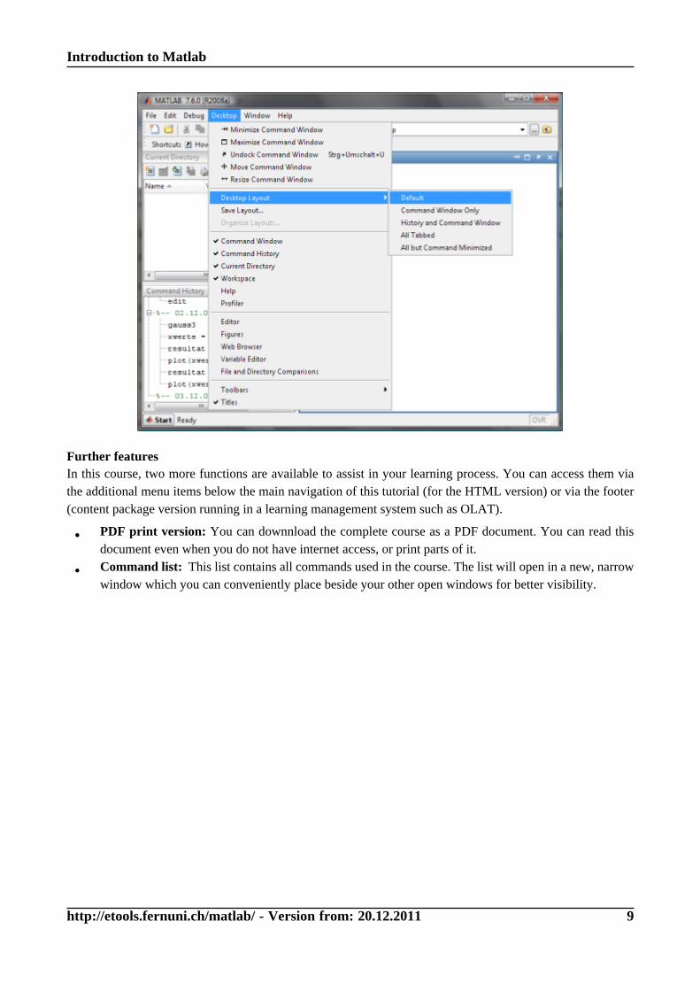
Special notationsMatlab expressions such as commands, functions, and other parts of the program code are highlighted withthe following text style:matlab_codeCalls to Matlab's menu functions are formatted like this:Desktop > Desktop Layout > DefaultThis, for example, indicates the operation:
Introduction to Matlab
http://etools.fernuni.ch/matlab/ - Version from: 20.12.2011 9
Further featuresIn this course, two more functions are available to assist in your learning process. You can access them viathe additional menu items below the main navigation of this tutorial (for the HTML version) or via the footer(content package version running in a learning management system such as OLAT).
• PDF print version: You can downnload the complete course as a PDF document. You can read thisdocument even when you do not have internet access, or print parts of it.
• Command list: This list contains all commands used in the course. The list will open in a new, narrowwindow which you can conveniently place beside your other open windows for better visibility.
Introduction to Matlab
http://etools.fernuni.ch/matlab/ - Version from: 20.12.2011 10
PreparationsThis section describes the preparatory steps necessary for doing this course:
• Installation of Matlab on your computer
• Downloading and saving of the necessary materials such as example programs, data files, and samplesolutions
• Configuration of Matlab
Introduction to Matlab
http://etools.fernuni.ch/matlab/ - Version from: 20.12.2011 11
Installation of Matlab
Which version of Matlab do I need?Version 7.2 / R2006a or newer is recommended. It is possible to use older versions; however, certain detailsof the user interface may be different. Basically, working with Matlab is substantially more pleasant with thenewer versions, especially due to useful extensions of the editor's functionality and improved help functions.For Matlab, a license has to be obtained. A student license is available from Mathworks for $99. Certainacademic institutions (e.g. University of Bern) make Matlab available for free to staff and students. Pleasecontact the IT support of your institution.
If Matlab has not been installed on your computer yet, do it now. Follow the instructions provided bythe installation program.
Important: Some versions of Matlab ask you to decide what exactly you want to install: the main application,the documentation, or both. Select both, as the documentation is an indispensable resource for working withthis complex program package.
Introduction to Matlab
http://etools.fernuni.ch/matlab/ - Version from: 20.12.2011 12
Downloading the necessary materials
To do this course, you need several data files such as code examples, sample solutions, or data files to test theprograms you have written. Thus, you are asked to download these files to your computer now.
Please download the data files now, as described below:
Examples and sample solutionsYou will find these program files in the ZIP archive file examples.zip. Please extract the contents to a newfolder (= directory), e.g. My Documents\matlab-course\m\ or d:\m\. It is useful to memoriseor write down the name of this folder, because we will have to configure it in Matlab right away (cf. here).Important: This folder will be your working folder for the programs you write.
DataSome of the examples and exercise assignments need data files. You can download them as ZIP archivedata.zip. Extract these files to another location, e.g. My Documents\matlab-course\data\.
Introduction to Matlab
http://etools.fernuni.ch/matlab/ - Version from: 20.12.2011 13
Configuration of Matlab
Several settings are necessary or helpful to make Matlab «operational»:
• setting the search path for your new programs
• configuration of the proxy server for internet access (if necessary)
• The tabulator size of the editor can be customised to suit one's taste.
Please follow these steps according to the instructions below. Afterwards you are ready to go!
Please check/configure the following settings:
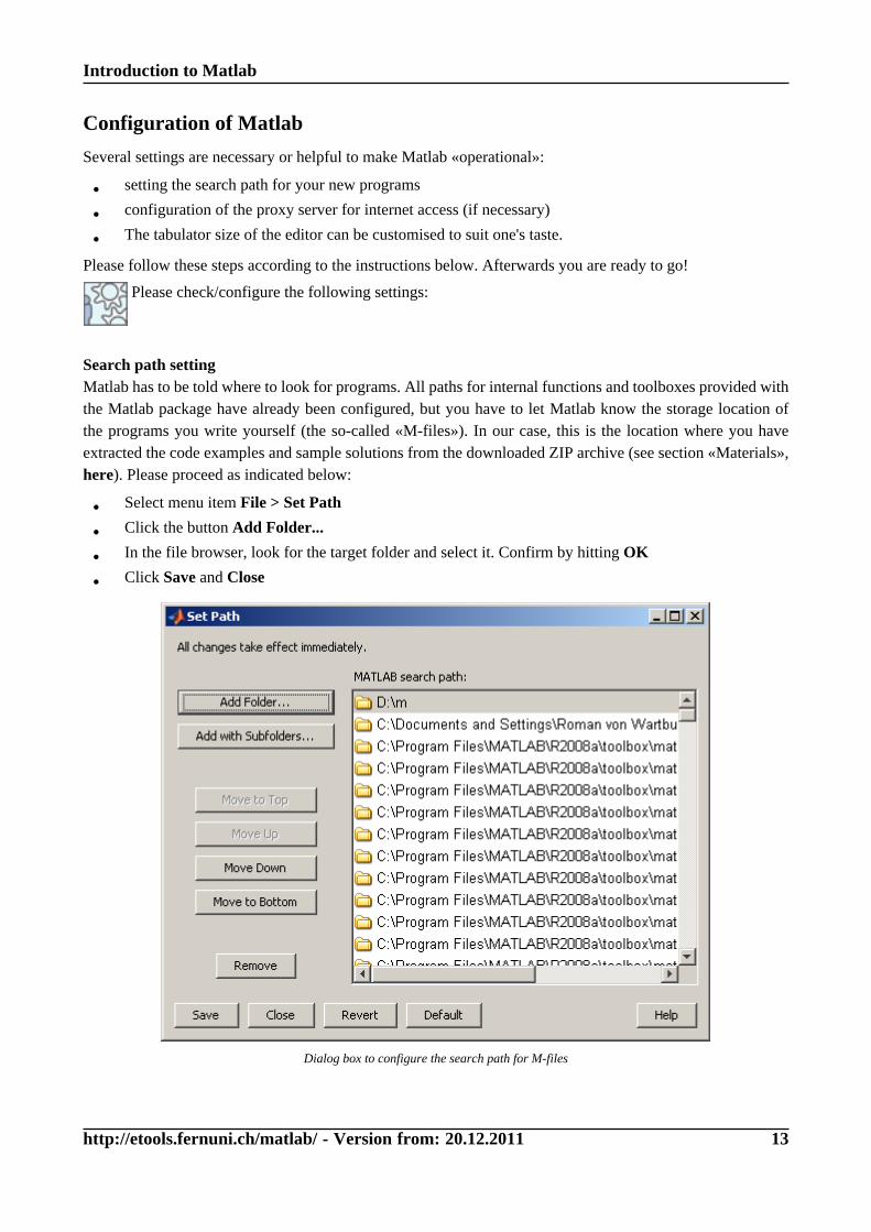
Search path settingMatlab has to be told where to look for programs. All paths for internal functions and toolboxes provided withthe Matlab package have already been configured, but you have to let Matlab know the storage location ofthe programs you write yourself (the so-called «M-files»). In our case, this is the location where you haveextracted the code examples and sample solutions from the downloaded ZIP archive (see section «Materials»,here). Please proceed as indicated below:
• Select menu item File > Set Path
• Click the button Add Folder...
• In the file browser, look for the target folder and select it. Confirm by hitting OK
• Click Save and Close
Dialog box to configure the search path for M-files
Introduction to Matlab
http://etools.fernuni.ch/matlab/ - Version from: 20.12.2011 14
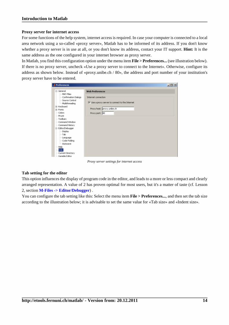
Proxy server for internet accessFor some functions of the help system, internet access is required. In case your computer is connected to a localarea network using a so-called «proxy server», Matlab has to be informed of its address. If you don't knowwhether a proxy server is in use at all, or you don't know its address, contact your IT support. Hint: It is thesame address as the one configured in your internet browser as proxy server.In Matlab, you find this configuration option under the menu item File > Preferences... (see illustration below).If there is no proxy server, uncheck «Use a proxy server to connect to the Internet». Otherwise, configure itsaddress as shown below. Instead of «proxy.unibe.ch / 80», the address and port number of your institution'sproxy server have to be entered.
Proxy server settings for internet access
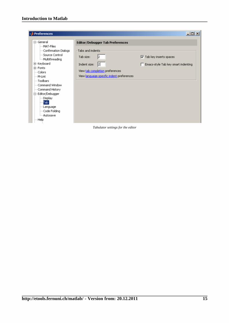
Tab setting for the editorThis option influences the display of program code in the editor, and leads to a more or less compact and clearlyarranged representation. A value of 2 has proven optimal for most users, but it's a matter of taste (cf. Lesson2, section M-Files -> Editor/Debugger) .You can configure the tab setting like this: Select the menu item File > Preferences..., and then set the tab sizeaccording to the illustration below; it is advisable to set the same value for «Tab size» and «Indent size».
Introduction to Matlab
http://etools.fernuni.ch/matlab/ - Version from: 20.12.2011 15
Tabulator settings for the editor

Introduction to Matlab
http://etools.fernuni.ch/matlab/ - Version from: 20.12.2011 16
Lesson 1: Matlab BasicsIn this lesson you'll get to know the features and possibilities provided by Matlab, and you learn how to interactwith Matlab by means of the user interface. Moreover, basic facts of data representation and manipulation areintroduced.
Learning Objectives
• You get an overview of what you can do with Matlab
• You know the different parts of the user interface
• You can adapt the user interface to your needs
• You know how to perform calculations in command line mode
• You get to know Matlab's basic methods to represents data (scalars, vectors, matrices)
• You can manipulate these data types and apply mathematical functions and operations to them.
Introduction to Matlab
http://etools.fernuni.ch/matlab/ - Version from: 20.12.2011 17
What Can You Use Matlab For?Below, an overview of the possibilities of Matlab is given. In case you already know the potential of Matlab,you can skip these sections and continue with The user interface.Matlab is short for Matrix laboratory. Matlab is a programming language and environment that makes use
of specialised data types (matrices 1, in particular).
In what cases is it advantageous to use Matlab?Small amounts of data that are acquired and evaluated only once can easily and efficiently be processed withspreadsheed software such as MS Excel or OpenOffice Calc. Afterwards they can be statistically analysed instatistics packages such as Statistica or SPSS. It is seldom worthwile to use Matlab for such tasks.The use of Matlab is more appropriate in the following cases:
• If you have to evaluate large amounts of data that are acquired automatically by means of computers
and other technical appliances. Examples are psychophysical experiments (EEG 2, fMRI 3, eye tracking,galvanic skin resistance measurements and the like), internet questionnaires, or log file analyses. In theseapplications, it is way too laborious to manually preprocess every single data set with a spreadsheetsoftware and export it to a statistics software package. Thus, automating this process by means of aMatlab program will be profitable.
• Moreover, the application of programmed data evaluation routines is a more efficient way if theevaluation procedure has to be changed over and over again to 'fine-tune' it. Re-calculating the wholedata set with the changed procedure is then done in a snap.
• Matlab offers a plethora of graphics functions, dedicated statistics functions and other interesting featureswhich are not available in other software packages, or only in limited and unflexible implementations.
• Matlab allows for the programming of user-friendly interfaces for data evaluation programs that arerepeatedly used. Thus, complicated data evaluation procedures can also be performed by collaboratorswho are less skilled with the computer.
Certainly, you can write data evaluation programs in other programming languages such as Visual Basic, C++, or Java, but Matlab is a language designed especially for processing, evaluating and graphical displaying ofnumerical data. A particular advantage of Matlab is that, contrary to most other languages, it can be used asan «interpreter»: you can enter single commands and have them executed immediately; in this way, you canquickly test how the syntax of the command has to be to yield the desired result. The thus verified commandscan then transferred by «copy-and-paste» to your program files. And to execute a program, you do not needto pre-process (compile) it beforehand.
Note to programmers: In spite of this user-friendly interface, Matlab programs are executed almostas fast as program code written in compiling languages such as C++ or Pascal. Moreover, it is evenpossible to compile Matlab programs and run them «stand alone».
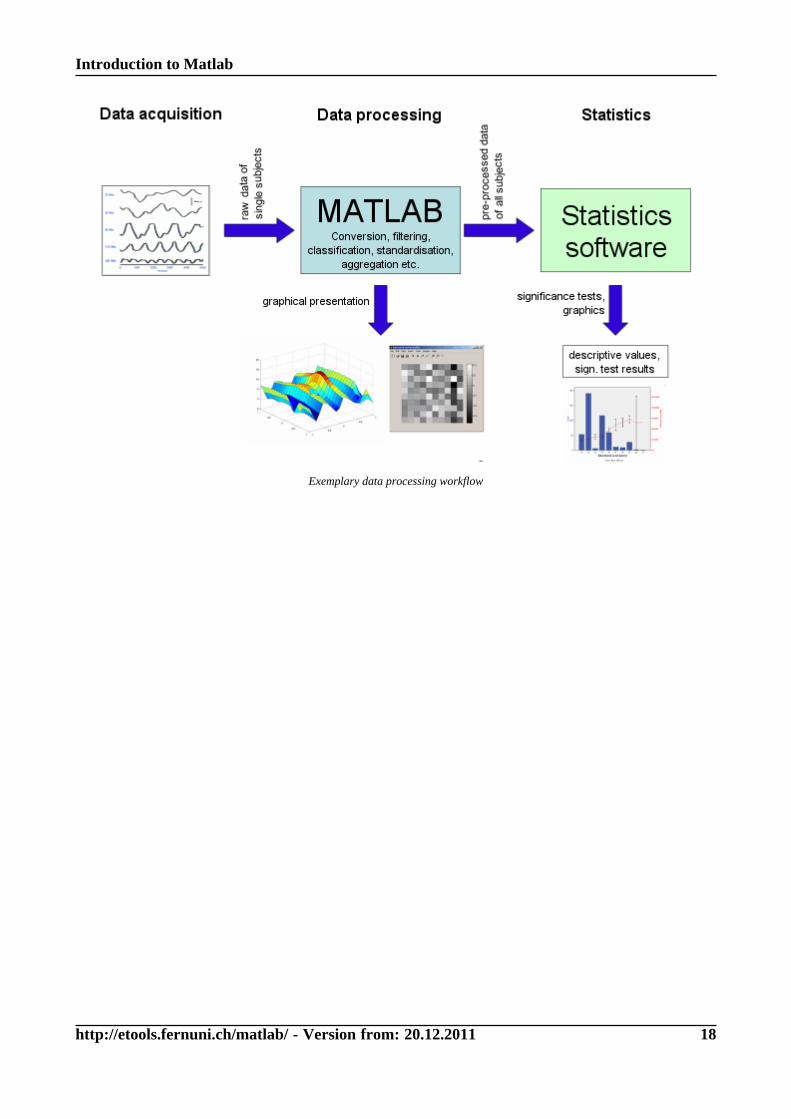
Typical data processing workflowBelow you see the schematic diagram of a typical project, showing which steps are often realised with Matlab.
1 The most important way to represent data in Matlab. In the field of mathematics, a matrix is a table of numbers or other values. Matrices
differ from ordinary tables in that they can be used for calculations. Usually, the expression «matrix» refers to two- or higher-dimensional
matrices (cf. scalar, vector).
Introduction to Matlab
http://etools.fernuni.ch/matlab/ - Version from: 20.12.2011 18
Exemplary data processing workflow
Introduction to Matlab
http://etools.fernuni.ch/matlab/ - Version from: 20.12.2011 19
Examples in Command Line Mode
Command line mode means that commands are directly entered in the «commandwindow» on the «command line», i.e. just after the command prompt >>. Matlab willthen execute them immediately, as opposed to programmed mode, i.e. a program iswritten first, and repeatedly executed later on (more on that subject see Lesson 2).
Now you can try out some of Matlab's features yourself. Start Matlab, enter the commands listed in the examplesbelow in the «command window» right behind the command prompt >>, and see what happens. For now, youdon't have to understand every command in detail; they will be explained later on in this course.
Example 1: The use of Matlab as a (somewhat oversized) «pocket calculator»
>> 27*5>> 2^10>> diameter=14.6>> circumference=diameter*pi>> area=diameter^2*pi/4>> ansExplanations: Simple calculations can be executed in the command line mode. If no variable name suchas diameter is noted, the result will be saved in the default variable ans (answer). pi is an internallypredefined variable that can be used at any time.
Example 2: Plotting a graph in command line mode
>> x = -pi:.01:pi>> y = sin(x)>> plot(x,y)>> hold on>> z = cos(x)>> plot(x,z,'r')Explanations: First, a sequence of values between -pi and pi with intervals of 0.01 is generated. Then, thesine values of these data are calculated. Subsequently, the results are plotted by means of the plot function.hold on «fixates» the graph so that it will not be deleted by the subsequent plot command. Additionally,the cosine values are calculated and plotted in red into the same graph.
Introduction to Matlab
http://etools.fernuni.ch/matlab/ - Version from: 20.12.2011 20
Afterwards, close the graphics window: Either in the usual way windows are closed, or by entering closeon the command line.
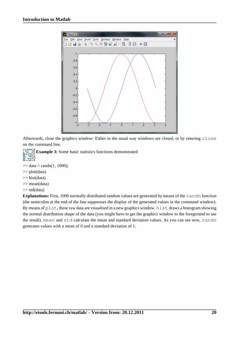
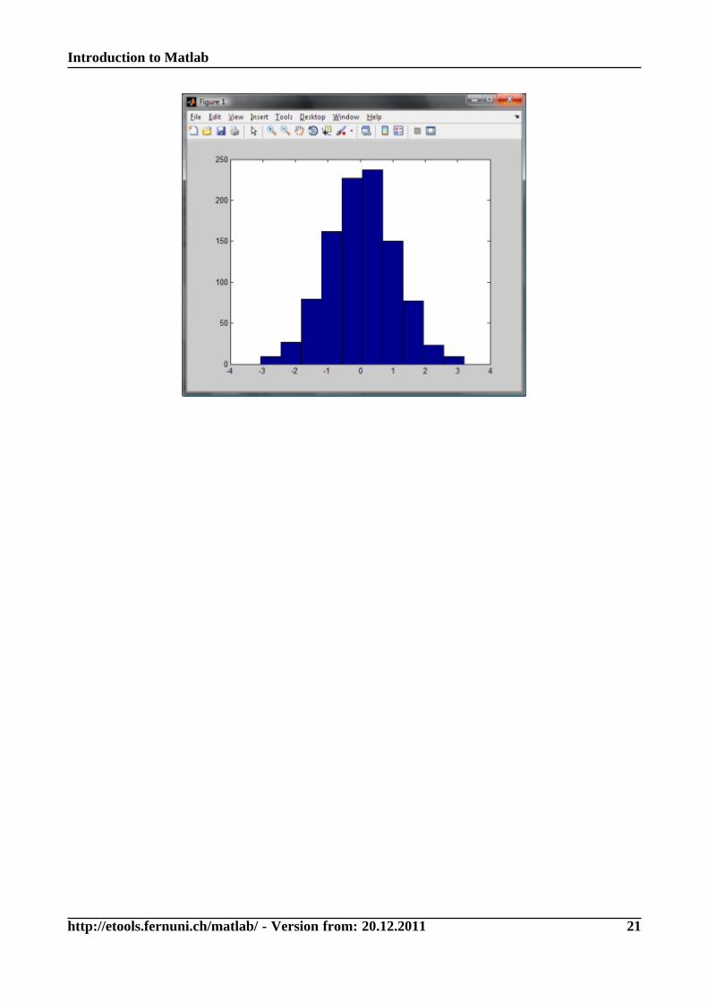
Example 3: Some basic statistics functions demonstrated
>> data = randn(1, 1000);>> plot(data)>> hist(data)>> mean(data)>> std(data)Explanations: First, 1000 normally distributed random values are generated by means of the randn function(the semicolon at the end of the line suppresses the display of the generated values in the command window).By means of plot, these raw data are visualised in a new graphics window. hist draws a histogram showingthe normal distribution shape of the data (you might have to get the graphics window to the foreground to seethe result). mean and std calculate the mean and standard deviation values. As you can see now, randngenerates values with a mean of 0 and a standard deviation of 1.
Introduction to Matlab
http://etools.fernuni.ch/matlab/ - Version from: 20.12.2011 21
Introduction to Matlab
http://etools.fernuni.ch/matlab/ - Version from: 20.12.2011 22
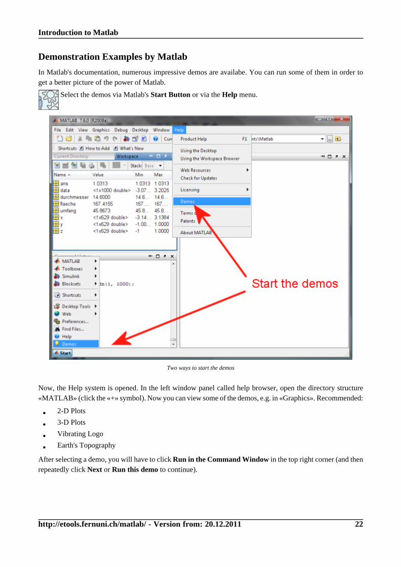
Demonstration Examples by Matlab
In Matlab's documentation, numerous impressive demos are availabe. You can run some of them in order toget a better picture of the power of Matlab.
Select the demos via Matlab's Start Button or via the Help menu.
Two ways to start the demos
Now, the Help system is opened. In the left window panel called help browser, open the directory structure«MATLAB» (click the «+» symbol). Now you can view some of the demos, e.g. in «Graphics». Recommended:
• 2-D Plots
• 3-D Plots
• Vibrating Logo
• Earth's Topography
After selecting a demo, you will have to click Run in the Command Window in the top right corner (and thenrepeatedly click Next or Run this demo to continue).
Introduction to Matlab
http://etools.fernuni.ch/matlab/ - Version from: 20.12.2011 23
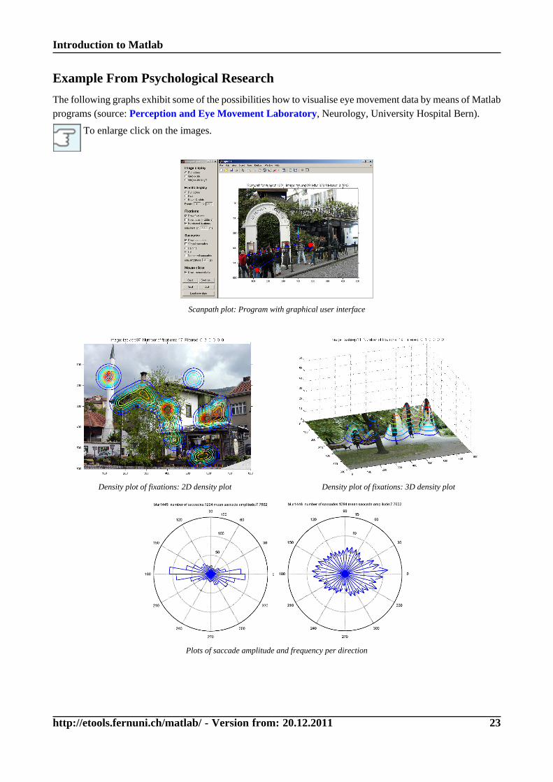
Example From Psychological Research
The following graphs exhibit some of the possibilities how to visualise eye movement data by means of Matlabprograms (source: Perception and Eye Movement Laboratory, Neurology, University Hospital Bern).
To enlarge click on the images.
Scanpath plot: Program with graphical user interface
Density plot of fixations: 2D density plot Density plot of fixations: 3D density plot
Plots of saccade amplitude and frequency per direction
Introduction to Matlab
http://etools.fernuni.ch/matlab/ - Version from: 20.12.2011 24
Only pictures can be viewed in this version! For Flash, animations, movies etc. see online version.Only screenshots of animations will be displayed. [link]
Animated scanpath display
Introduction to Matlab
http://etools.fernuni.ch/matlab/ - Version from: 20.12.2011 25
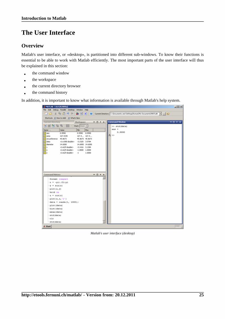
The User Interface
Overview
Matlab's user interface, or «desktop», is partitioned into different sub-windows. To know their functions isessential to be able to work with Matlab efficiently. The most important parts of the user interface will thusbe explained in this section:
• the command window
• the workspace
• the current directory browser
• the command history
In addition, it is important to know what information is available through Matlab's help system.
Matlab's user interface (desktop)
Introduction to Matlab
http://etools.fernuni.ch/matlab/ - Version from: 20.12.2011 26
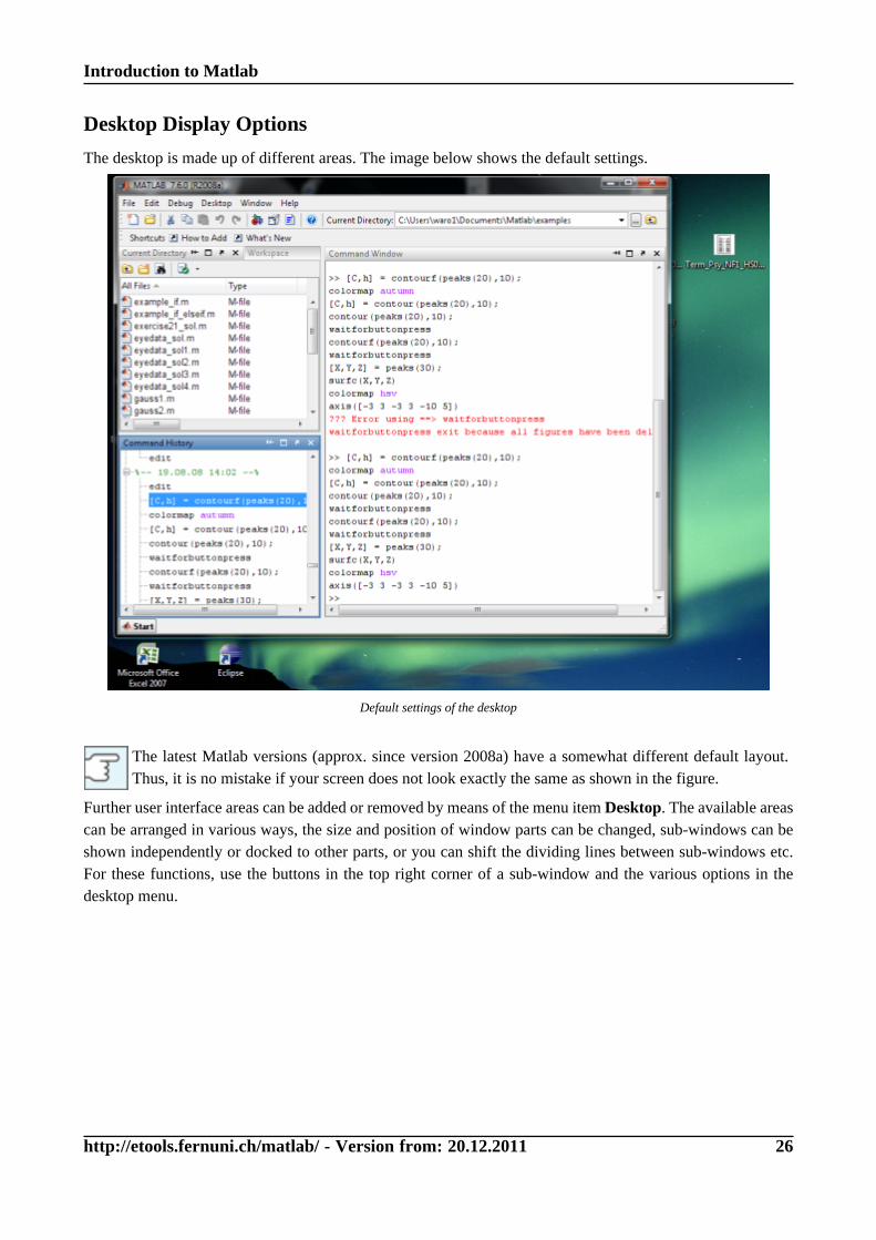
Desktop Display Options
The desktop is made up of different areas. The image below shows the default settings.
Default settings of the desktop
The latest Matlab versions (approx. since version 2008a) have a somewhat different default layout.Thus, it is no mistake if your screen does not look exactly the same as shown in the figure.
Further user interface areas can be added or removed by means of the menu item Desktop. The available areascan be arranged in various ways, the size and position of window parts can be changed, sub-windows can beshown independently or docked to other parts, or you can shift the dividing lines between sub-windows etc.For these functions, use the buttons in the top right corner of a sub-window and the various options in thedesktop menu.
Introduction to Matlab
http://etools.fernuni.ch/matlab/ - Version from: 20.12.2011 27
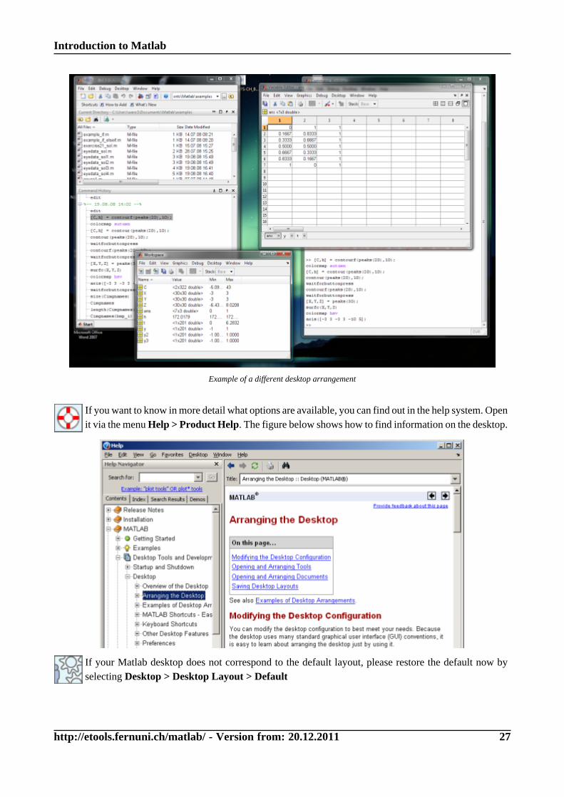
Example of a different desktop arrangement
If you want to know in more detail what options are available, you can find out in the help system. Openit via the menu Help > Product Help. The figure below shows how to find information on the desktop.
If your Matlab desktop does not correspond to the default layout, please restore the default now byselecting Desktop > Desktop Layout > Default
Introduction to Matlab
http://etools.fernuni.ch/matlab/ - Version from: 20.12.2011 28
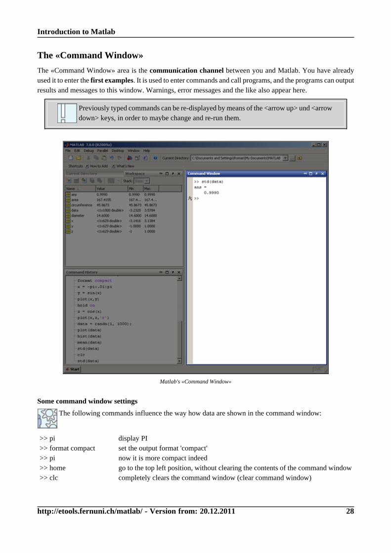
The «Command Window»
The «Command Window» area is the communication channel between you and Matlab. You have alreadyused it to enter the first examples. It is used to enter commands and call programs, and the programs can outputresults and messages to this window. Warnings, error messages and the like also appear here.
Previously typed commands can be re-displayed by means of the <arrow up> und <arrowdown> keys, in order to maybe change and re-run them.
Matlab's «Command Window»
Some command window settings
The following commands influence the way how data are shown in the command window:
>> pi>> format compact>> pi>> home>> clc
display PIset the output format 'compact'now it is more compact indeedgo to the top left position, without clearing the contents of the command windowcompletely clears the command window (clear command window)
Introduction to Matlab
http://etools.fernuni.ch/matlab/ - Version from: 20.12.2011 29
Explanations: The command format changes the display of values in the command window in manyfoldways. format compact disables the output of superfluous empty lines. For further options please referto the information in the help system (e.g. by typing docsearch format in the command window).
Introduction to Matlab
http://etools.fernuni.ch/matlab/ - Version from: 20.12.2011 30
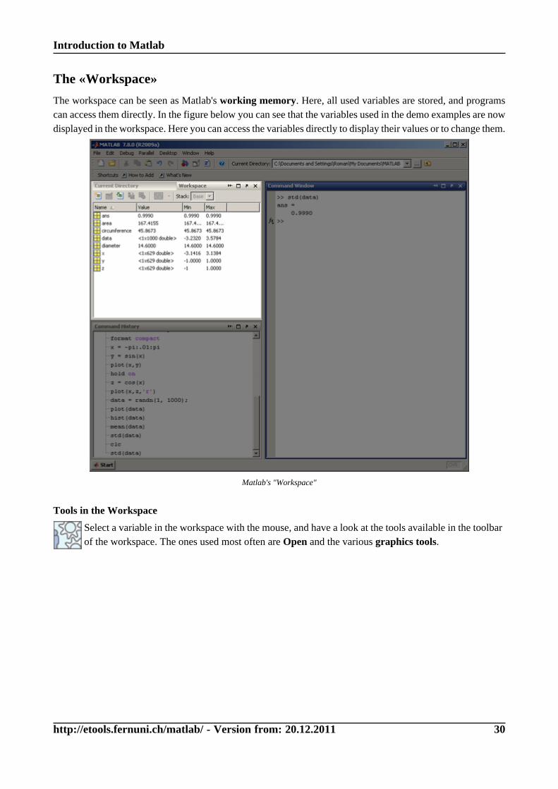
The «Workspace»
The workspace can be seen as Matlab's working memory. Here, all used variables are stored, and programscan access them directly. In the figure below you can see that the variables used in the demo examples are nowdisplayed in the workspace. Here you can access the variables directly to display their values or to change them.
Matlab's "Workspace"
Tools in the Workspace
Select a variable in the workspace with the mouse, and have a look at the tools available in the toolbarof the workspace. The ones used most often are Open and the various graphics tools.
Introduction to Matlab
http://etools.fernuni.ch/matlab/ - Version from: 20.12.2011 31
Introduction to Matlab
http://etools.fernuni.ch/matlab/ - Version from: 20.12.2011 32
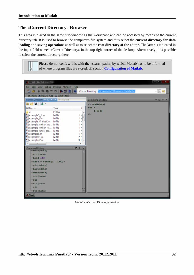
The «Current Directory» Browser
This area is placed in the same sub-window as the workspace and can be accessed by means of the currentdirectory tab. It is used to browse the computer's file system and thus select the current directory for dataloading and saving operations as well as to select the root directory of the editor. The latter is indicated inthe input field named «Current Directory» in the top right corner of the desktop. Alternatively, it is possibleto select the current directory there.
Please do not confuse this with the «search path», by which Matlab has to be informedof where program files are stored, cf. section Configuration of Matlab.
Matlab's «Current Directory» window
Introduction to Matlab
http://etools.fernuni.ch/matlab/ - Version from: 20.12.2011 33
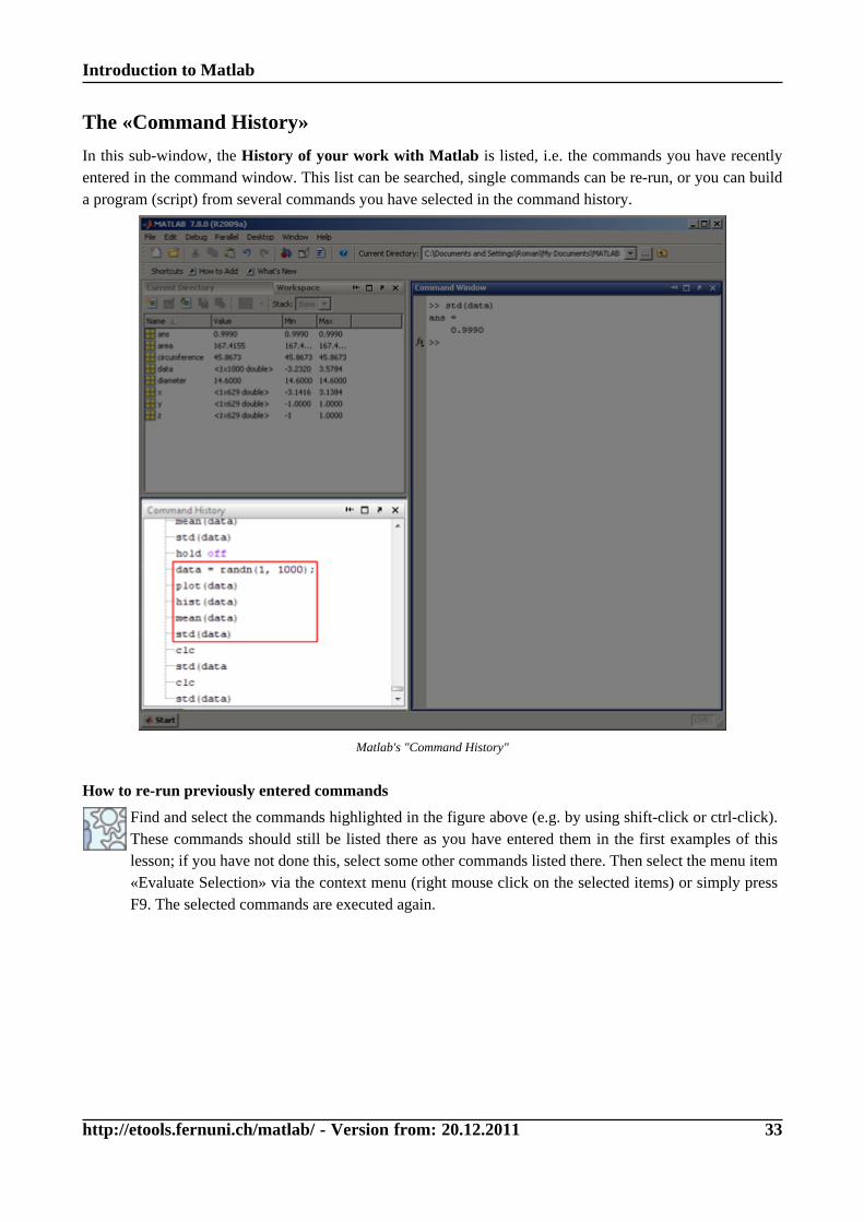
The «Command History»
In this sub-window, the History of your work with Matlab is listed, i.e. the commands you have recentlyentered in the command window. This list can be searched, single commands can be re-run, or you can builda program (script) from several commands you have selected in the command history.
Matlab's "Command History"
How to re-run previously entered commands
Find and select the commands highlighted in the figure above (e.g. by using shift-click or ctrl-click).These commands should still be listed there as you have entered them in the first examples of thislesson; if you have not done this, select some other commands listed there. Then select the menu item«Evaluate Selection» via the context menu (right mouse click on the selected items) or simply pressF9. The selected commands are executed again.
Introduction to Matlab
http://etools.fernuni.ch/matlab/ - Version from: 20.12.2011 34
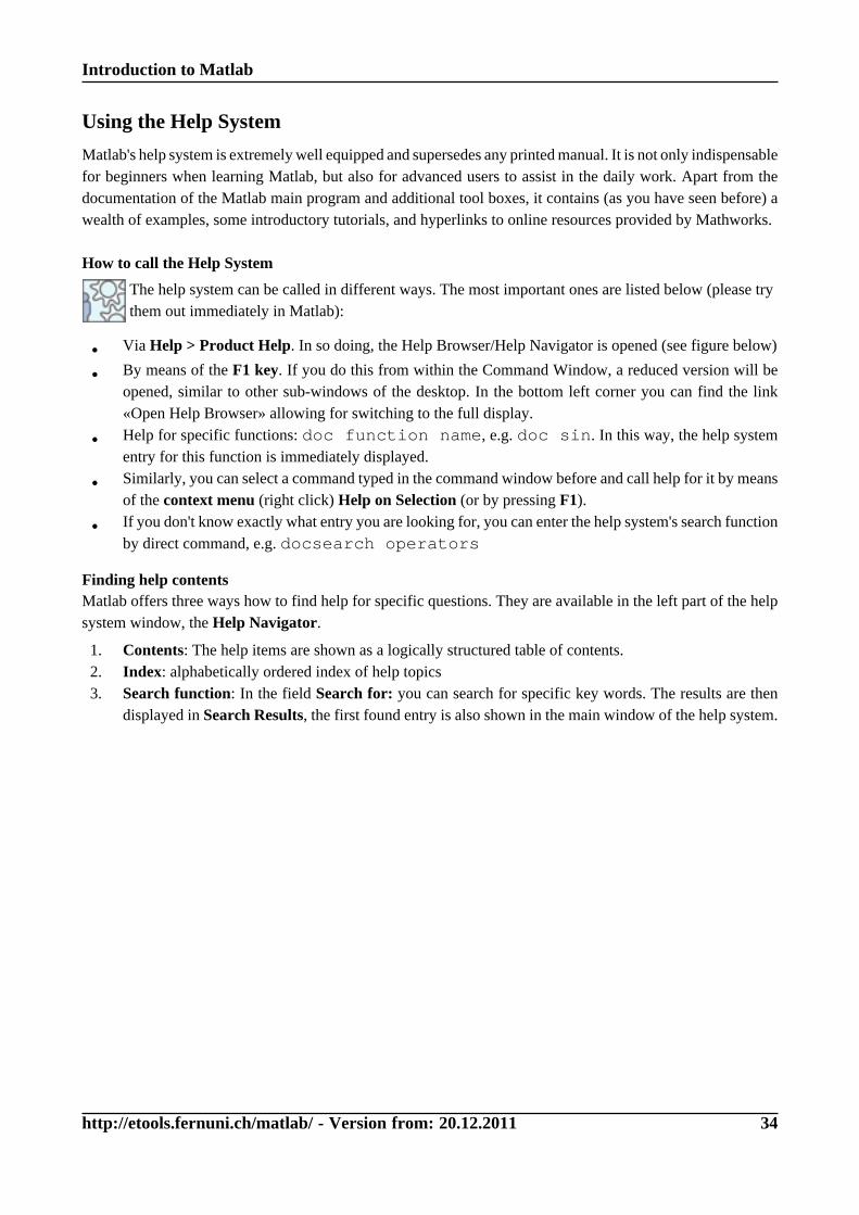
Using the Help System
Matlab's help system is extremely well equipped and supersedes any printed manual. It is not only indispensablefor beginners when learning Matlab, but also for advanced users to assist in the daily work. Apart from thedocumentation of the Matlab main program and additional tool boxes, it contains (as you have seen before) awealth of examples, some introductory tutorials, and hyperlinks to online resources provided by Mathworks.
How to call the Help System
The help system can be called in different ways. The most important ones are listed below (please trythem out immediately in Matlab):
• Via Help > Product Help. In so doing, the Help Browser/Help Navigator is opened (see figure below)
• By means of the F1 key. If you do this from within the Command Window, a reduced version will beopened, similar to other sub-windows of the desktop. In the bottom left corner you can find the link«Open Help Browser» allowing for switching to the full display.
• Help for specific functions: doc function name, e.g. doc sin. In this way, the help systementry for this function is immediately displayed.
• Similarly, you can select a command typed in the command window before and call help for it by meansof the context menu (right click) Help on Selection (or by pressing F1).
• If you don't know exactly what entry you are looking for, you can enter the help system's search functionby direct command, e.g. docsearch operators
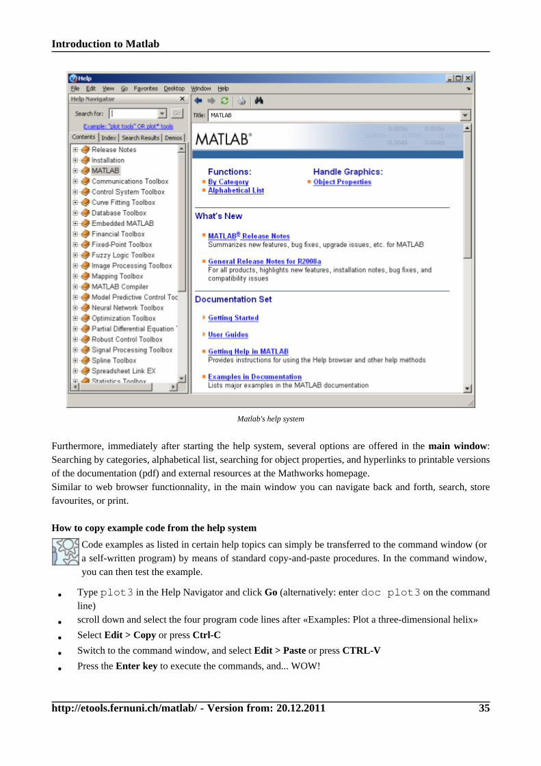
Finding help contentsMatlab offers three ways how to find help for specific questions. They are available in the left part of the helpsystem window, the Help Navigator.
1. Contents: The help items are shown as a logically structured table of contents.2. Index: alphabetically ordered index of help topics3. Search function: In the field Search for: you can search for specific key words. The results are then
displayed in Search Results, the first found entry is also shown in the main window of the help system.
Introduction to Matlab
http://etools.fernuni.ch/matlab/ - Version from: 20.12.2011 35
Matlab's help system
Furthermore, immediately after starting the help system, several options are offered in the main window:Searching by categories, alphabetical list, searching for object properties, and hyperlinks to printable versionsof the documentation (pdf) and external resources at the Mathworks homepage.Similar to web browser functionnality, in the main window you can navigate back and forth, search, storefavourites, or print.
How to copy example code from the help system
Code examples as listed in certain help topics can simply be transferred to the command window (ora self-written program) by means of standard copy-and-paste procedures. In the command window,you can then test the example.
• Type plot3 in the Help Navigator and click Go (alternatively: enter doc plot3 on the commandline)
• scroll down and select the four program code lines after «Examples: Plot a three-dimensional helix»
• Select Edit > Copy or press Ctrl-C
• Switch to the command window, and select Edit > Paste or press CTRL-V
• Press the Enter key to execute the commands, and... WOW!
Introduction to Matlab
http://etools.fernuni.ch/matlab/ - Version from: 20.12.2011 36
Summary
The most important contents of the section «The User Interface» are summarised below.
• The «Command Window» area is the communication channel between the userand the Matlab program. Here, commands can be entered, and programs can outputresults and messages. Warnings, error messages and the like are also shown here.
• In the Command Window, previously entered commands can be repeated with thekeys <arrow up> and <arrow down>, and then changed and re-executed.
• The «Workspace» is the working memory of Matlab. It stores the used variableson which programs operate.
• The «Current Directory» browser is used to access the computer's file system.There, you can select the current directory for data storage as well as the rootdirectory for the editor.
• In the window «Command History» you find the commands you have enteredthroughout the current session in the command window.
• Matlab's help system is an indispensable aid for beginners as well as experiencedusers. It makes a printed manual unnecessary.
Introduction to Matlab
http://etools.fernuni.ch/matlab/ - Version from: 20.12.2011 37
Numbers and Variables in MatlabAs you have seen in section Why Matlab?, calculations, graphical displays etc. can be performed in a simpleway in the command line mode, i.e. by directly typing commands in the Command Window.In the next sections you can learn the basics that are necessary to work in the command line mode:
• How are numbers represented in Matlab?
• What are variables?
• The most important data type: the matrix
• How to work with matrices
• What operators and functions can be used for calculations?
These points not only pertain to the command line mode, but also to self-written programs, as you will learnin Lesson 2: Programming in MatlabUsing the command line mode allows for testing commands before including them in a program, which isuseful in case you are not sure of their syntax or function.
Introduction to Matlab
http://etools.fernuni.ch/matlab/ - Version from: 20.12.2011 38
Representation of Numbers
As usual in English, numbers with decimal places are written with a period. The comma is used to separateconsecutive commands on the same line. The result of an operation (below it will only be entering a number)is assigned to the predefined variable ans (answer), unless it is explicitely assigned to a specific variable.
Please enter the commands listed below in the Command Window and try to understand what Matlabdoes with your inputs.
>> format compact>> 23.736>> 784,400>> pi
activate compact displaycorrectly entered numberthis is interpreted as TWO numbers, separated by the commai.e. you must not write large integer numbers with commaspi is a pre-defined constant, that can be used at any time
For numbers in scientific notation, the letter e is used to separate the exponent (to the base of 10). Examples:
>> 1.746e5>> 584e-11
for 1.746 x 10⁵
of course, negative exponents are allowed as well
Contrary to other programming languages, Matlab has representations for two special values: infinite (inf) and«not a number» (NaN). These values can be the result of calculations, such as division by zero, and can assuch also be assigned to a variable.
Please try out the following commands that illustrate this.
>> 2/0>> -5/0>> 0/0>> inf/inf>> 0*inf
division by 0 yields infminus infinite is also possible0 devided by 0 results in NaN
Introduction to Matlab
http://etools.fernuni.ch/matlab/ - Version from: 20.12.2011 39
Variables
Data are stored in Matlab's working memory (i.e. the workspace) as variables.
A variable is a reserved «place» in computer memory that can be referenced with a uniquename.A variable can contain various kinds of data. This fact is expressed by saying that avariable is of a certain data type (or just «type»).
Examples for data types are simple numbers, matrices, character sequences (strings), structured data etc.In the examples below we only use simple numbers. You will get to know further data types later on in thiscourse.Contrary to many other programming langauges, variables do not have to be pre-defined (i.e. to reserve thenecessary memory space for them). Matlab will automatically reserve the memory space at the time of theirfirst usage, that is when they are assigned a value for the first time.
Variable naming conventionsA variable is identified by a unique name. The name has to begin with a letter, after that it can contain furtherletters, numbers, or the «underscore» _.Variable names are case-sensitive, i.e. capitalising is relevant.
In the examples below you can see what variable names are allowed, how variables can be filled withvalues, and how these values can be recalled again.
>> Speed = 63>> g65_fubar = 3>> Speed>> speed>> 6test = 2>> _foo = 1>> hi$there>> pi = 11>> sin = 0
the equal sign assigns a value to a variableanother valid namerecall the valuethis does not work when spelt lowercasea name not starting with a letter is invaliddittothe only special character allowed is the underscore _It is even possible to redefine pre-defined constants like pi or function names(here, the sine function sin), but has to be used with care (or better not at all)...
Loading and saving variables in the WorkspaceAlle variables that have been used are visible in the Workspace. The contents of the Workspace can be savedto the hard disk with save (to the folder that is selected in the Current Directory Browser window) andloaded back from the hard disk by using load.Single variables can be removed from the Workspace with the clear command.
Please try it out again by yourself:
>> save data>> clear Speed>> clear>> load data
saves all variables to the file data.matnow the variable Speed is no longer in the Workspacedeletes all variables (note the Workspace window)loads back the variables from the file (see the Workspace window)
Introduction to Matlab
http://etools.fernuni.ch/matlab/ - Version from: 20.12.2011 40
Saving and loading workspace variables can also be done by means of the menu buttons of the Workspacewindow. Single variables can directly be deleted in the Workspace (select the variable and hit the 'delete' keyor use context menu > delete).
Introduction to Matlab
http://etools.fernuni.ch/matlab/ - Version from: 20.12.2011 41
Summary
In the following, you find a brief summary of the most important points of the section«Numbers and Variables».
• Decimal places of a number are separated by a period.
• Scientific notation is spelt with e, for instance 2.7e6 for 2.7 x 10 6.
• In Matlab, operations such as division by zero, that are not allowed in otherprogramming languages or applications, result in defined values such as inf forinfinite or NaN für «not a number».
• A variable is referenced by a unique name. It has to begin with a letter and cancontain more letters, numbers or the «underscore» _.
• Variable names are case-sensitive.
Introduction to Matlab
http://etools.fernuni.ch/matlab/ - Version from: 20.12.2011 42
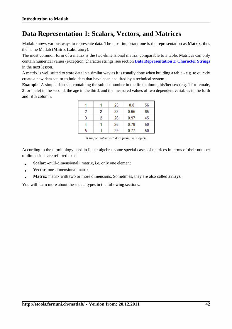
Data Representation 1: Scalars, Vectors, and MatricesMatlab knows various ways to represente data. The most important one is the representation as Matrix, thusthe name Matlab (Matrix Laboratory).The most common form of a matrix is the two-dimensional matrix, comparable to a table. Matrices can onlycontain numerical values (exception: character strings, see section Data Representation 1: Character Stringsin the next lesson.A matrix is well suited to store data in a similar way as it is usually done when building a table - e.g. to quicklycreate a new data set, or to hold data that have been acquired by a technical system.Example: A simple data set, containing the subject number in the first column, his/her sex (e.g. 1 for female,2 for male) in the second, the age in the third, and the measured values of two dependent variables in the forthand fifth column.
A simple matrix with data from five subjects
According to the terminology used in linear algebra, some special cases of matrices in terms of their numberof dimensions are referred to as:
• Scalar: «null-dimensional» matrix, i.e. only one element
• Vector: one-dimensional matrix
• Matrix: matrix with two or more dimensions. Sometimes, they are also called arrays.
You will learn more about these data types in the following sections.
Introduction to Matlab
http://etools.fernuni.ch/matlab/ - Version from: 20.12.2011 43
Scalars
A scalar is a matrix with one row and one column, and thus only contains a single numerical value.
The notation with square brackets [ ] always designates a matrix, including scalars andvectors! (with one exception, see section Programming of Functions, Example 3).
Please try this out yourself:
>> sc = 93>> sc2 = [13]>> sc(1,1)>> isscalar(sc)
This is a scalar. Thus, the square brackets are not mandatory here.more general notation as 1x1 matrixis identical to sc - the element in row 1, column 1determines whether sc is a scalar (1 = yes, 0 = no)
Introduction to Matlab
http://etools.fernuni.ch/matlab/ - Version from: 20.12.2011 44
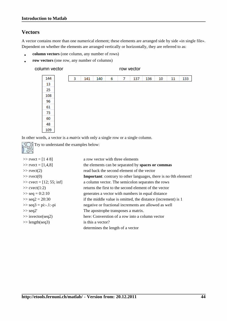
Vectors
A vector contains more than one numerical element; these elements are arranged side by side «in single file».Dependent on whether the elements are arranged vertically or horizontally, they are referred to as:
• column vectors (one column, any number of rows)
• row vectors (one row, any number of columns)
In other words, a vector is a matrix with only a single row or a single column.
Try to understand the examples below:
>> rvect = [1 4 8]>> rvect = [1,4,8]>> rvect(2)>> rvect(0)>> cvect = [12; 55; inf]>> cvect(1:2)>> seq = 0:2:10>> seq2 = 20:30>> seq3 = pi:-.1:-pi>> seq2'>> isvector(seq2)>> length(seq3)
a row vector with three elementsthe elements can be separated by spaces or commasread back the second element of the vectorImportant: contrary to other languages, there is no 0th element!a column vector. The semicolon separates the rowsreturns the first to the second element of the vectorgenerates a vector with numbers in equal distanceif the middle value is omitted, the distance (increment) is 1negative or fractional increments are allowed as wellThe apostrophe transposes a matrix.here: Converstion of a row into a column vectoris this a vector?determines the length of a vector
Introduction to Matlab
http://etools.fernuni.ch/matlab/ - Version from: 20.12.2011 45
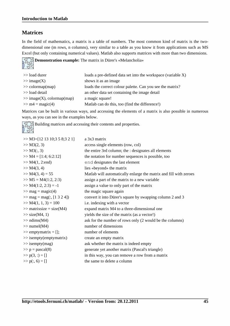
Matrices
In the field of mathematics, a matrix is a table of numbers. The most common kind of matrix is the two-dimensional one (m rows, n columns), very similar to a table as you know it from applications such as MSExcel (but only containing numerical values). Matlab also supports matrices with more than two dimensions.
Demonstration example: The matrix in Dürer's «Melancholia»
>> load durer>> image(X)>> colormap(map)>> load detail>> image(X), colormap(map)>> m4 = magic(4)
loads a pre-defined data set into the workspace (variable X)shows it as an imageloads the correct colour palette. Can you see the matrix?an other data set containing the image detaila magic square!Matlab can do this, too (find the difference!)
Matrices can be built in various ways, and accessing the elements of a matrix is also possible in numerousways, as you can see in the examples below.
Building matrices and accessing their contents and properties.
>> M3=[12 13 10;3 5 8;3 2 1]>> M3(2, 3)>> M3(:, 3)>> M4 = [1:4; 6:2:12]>> M4(1, 2:end)>> M4(3, 4)>> M4(3, 4) = 55>> M5 = M4(1:2, 2:3)>> M4(1:2, 2:3) = -1>> mag = magic(4)>> mag = mag(:, [1 3 2 4])>> M4(1, 1, 3) = 100>> matrixsize = size(M4)>> size(M4, 1)>> ndims(M4)>> numel(M4)>> emptymatrix = [];>> isempty(emptymatrix)>> isempty(mag)>> p = pascal(8)>> p(3, :) = []>> p(:, 6) = []
a 3x3 matrixaccess single elements (row, col)the entire 3rd column; the : designates all elementsthe notation for number sequences is possible, tooend designates the last elementlies «beyond» the matrixMatlab will automatically enlarge the matrix and fill with zeroesassign a part of the matrix to a new variableassign a value to only part of the matrixthe magic square againconvert it into Dürer's square by swapping column 2 and 3i.e. indexing with a vectorexpand matrix M4 to a three-dimensional oneyields the size of the matrix (as a vector!)ask for the number of rows only (2 would be the columns)number of dimensionsnumber of elementscreate an empty matrixask whether the matrix is indeed emptygenerate yet another matrix (Pascal's triangle)in this way, you can remove a row from a matrixthe same to delete a column
Introduction to Matlab
http://etools.fernuni.ch/matlab/ - Version from: 20.12.2011 46
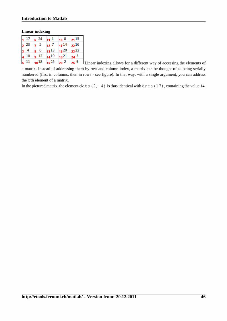
Linear indexing
Linear indexing allows for a different way of accessing the elements ofa matrix. Instead of addressing them by row and column index, a matrix can be thought of as being seriallynumbered (first in columns, then in rows - see figure). In that way, with a single argument, you can addressthe x'th element of a matrix.In the pictured matrix, the element data(2, 4) is thus identical with data(17), containing the value 14.
Introduction to Matlab
http://etools.fernuni.ch/matlab/ - Version from: 20.12.2011 47
Summary
Below, you again find the most important points in a brief summary. Additionally,relevant Matlab commands are listed.
Points to remember
• A scalar is a matrix with one row and one column, that is with only a singlenumerical value.
• A vector is a matrix with a single row (row vector) or a single column (columnvector).
• The most common matrix is the two-dimensional matrix (m rows, n columns).Matlab also allows for higher-dimensional matrices, e.g. with m rows, n columnsand p planes.
• When defining matrices and vectors, the elements have to be enclosed in squarebrackets [ ]. For scalars, the brackets are optional.
• The elements of matrices and vectors that belong to the same row are separatedwith a space or comma. The semicolon separates rows.
• Number sequences (= vectors) can be produced with the : - notation, e.g.10:2:50 for all even numbers from 10 to 50.
• A solitary colon designates all elements of a row or column, e.g. data(:, 12)for all rows, but only column 12 of the matrix.
• When indexing elements of a matrix, the indices are enclosed in round brackets( ).
• The indices always run from 1 to n, the index 0 (the «zeroth» element) does notexist in Matlab.
• In two-dimensional matrices, the first index is the row, the second one is thecolumn.
• Linear indexing: Instead of addressing elements by row and column index, a matrixcan be seen as being serially numbered; thus you can address the x'th element ofa matrix with a single argument.
Commands
• isscalar, isvector: check whether a variable is a scalar or a vector,respectively
• length determines the length of a vector
• ndims returns the dimensionality (number of dimensions) of a matrix
• numel calculates the total number of elements of a matrix
• size returns the size of a matrix
• isempty determines whether a matrix is empty
Introduction to Matlab
http://etools.fernuni.ch/matlab/ - Version from: 20.12.2011 48
Matrix ManipulationIn this section, you learn various possibilities to manipulate Matrices:
• matrix concatenation
• matrix duplication
• creating special matrices
• matrix transformation
This section will be concluded with a first practical exercise.
Introduction to Matlab
http://etools.fernuni.ch/matlab/ - Version from: 20.12.2011 49
Matrix Concatenation
Matrices can be concatenated with the normal [ ] -notation.
Please try to comprehend this by following the examples below:
>> a = magic(5);>> b = randn(5,3);>> c = [a b]>> d = [a; b]>> b = randn(5,5);>> d = [a; b]>> e = [a, d, a]
the semicolon prevents the output of a in the Command Windowrandom numbers, 5 rows, 3 columnshorizontal concatenationvertical concatenation: does not work this way because the number of columnsis inequalthus, we convert b into a 5x5 matrixnow it worksyou can also concatenate more than two matrices at once
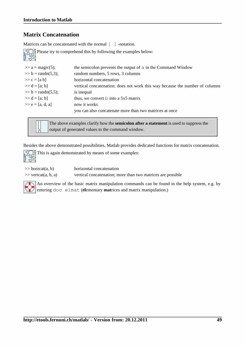
The above examples clarify how the semicolon after a statement is used to suppress theoutput of generated values to the command window.
Besides the above demonstrated possibilities, Matlab provides dedicated functions for matrix concatenation.
This is again demonstrated by means of some examples:
>> horzcat(a, b)>> vertcat(a, b, a)
horizontal concatenationvertical concatenation; more than two matrices are possible
An overview of the basic matrix manipulation commands can be found in the help system, e.g. byentering doc elmat (elementary matrices and matrix manipulation.)
Introduction to Matlab
http://etools.fernuni.ch/matlab/ - Version from: 20.12.2011 50
Matrix Duplication
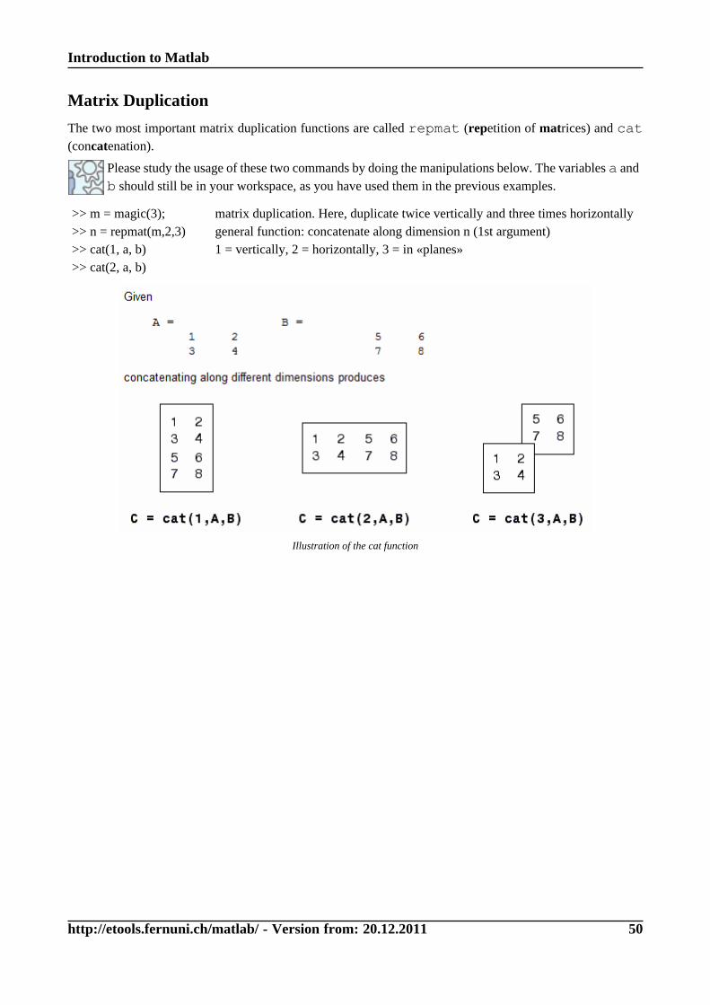
The two most important matrix duplication functions are called repmat (repetition of matrices) and cat(concatenation).
Please study the usage of these two commands by doing the manipulations below. The variables a andb should still be in your workspace, as you have used them in the previous examples.
>> m = magic(3);>> n = repmat(m,2,3)>> cat(1, a, b)>> cat(2, a, b)
matrix duplication. Here, duplicate twice vertically and three times horizontallygeneral function: concatenate along dimension n (1st argument)1 = vertically, 2 = horizontally, 3 = in «planes»
Illustration of the cat function
Introduction to Matlab
http://etools.fernuni.ch/matlab/ - Version from: 20.12.2011 51
Creation of Special Matrices
Certain special matrices are needed again and again, thus Matlab provides commands to create such matrices.Some examples:
• Matrices filled with zeroes or ones
• Matrices with random numbers with different distributions. This can sometimes be helpful to teststatistical functions or generate test data sets. Also see Random Numbers in Lesson 4
• Particular matrices for linear algebra: identity matrix, Pascal's triangle etc.
In the examples below, you can see the most important ones of these functions.
>> zeros(7, 3)>> allones = ones(4)>> a(1:5, 1:10) = 3.5>> b = ones(7, 3) * 81>> rand(1, 8)>> randn(2, 6)>> eye(5)>> pascal(7)>> magic(8)
Matrix with zeroesMatrix with ones. If only one argument is given, a square matrix resultsTo create a matrix with other values, there are several ways.random numbers between 0 and 1normally distributed random numbers with a mean of 0and a standard deviation of 1so-called identity matrix (only square matrix is possible), linear algebraPascal's triangle matrix, a thing more for mathematiciansmagic squares
Introduction to Matlab
http://etools.fernuni.ch/matlab/ - Version from: 20.12.2011 52
Matrix Transformation
The most important transformations are:
• Mirroring (horizontally or vertically)
• Rotation
• Transposition (swap rows and columns)
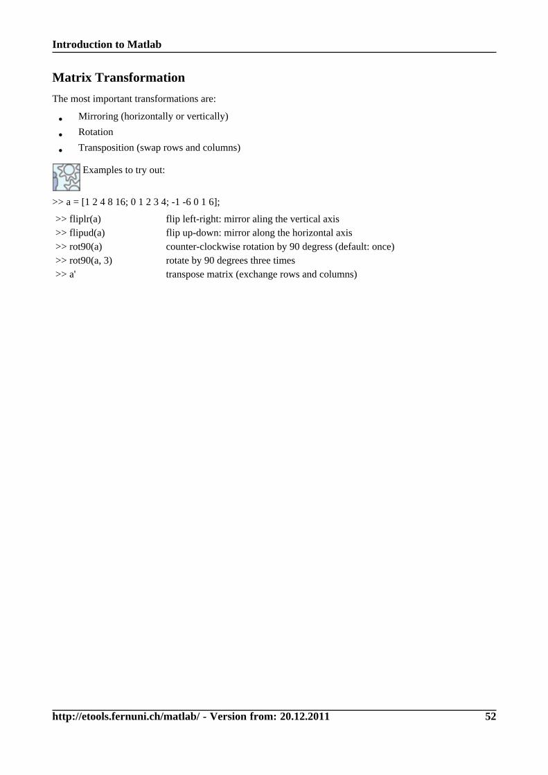
Examples to try out:
>> a = [1 2 4 8 16; 0 1 2 3 4; -1 -6 0 1 6];
>> fliplr(a)>> flipud(a)>> rot90(a)>> rot90(a, 3)>> a'
flip left-right: mirror aling the vertical axisflip up-down: mirror along the horizontal axiscounter-clockwise rotation by 90 degress (default: once)rotate by 90 degrees three timestranspose matrix (exchange rows and columns)
Introduction to Matlab
http://etools.fernuni.ch/matlab/ - Version from: 20.12.2011 53
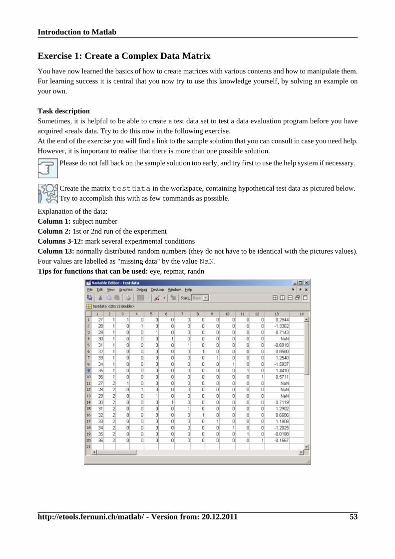
Exercise 1: Create a Complex Data Matrix
You have now learned the basics of how to create matrices with various contents and how to manipulate them.For learning success it is central that you now try to use this knowledge yourself, by solving an example onyour own.
Task descriptionSometimes, it is helpful to be able to create a test data set to test a data evaluation program before you haveacquired «real» data. Try to do this now in the following exercise.At the end of the exercise you will find a link to the sample solution that you can consult in case you need help.However, it is important to realise that there is more than one possible solution.
Please do not fall back on the sample solution too early, and try first to use the help system if necessary.
Create the matrix testdata in the workspace, containing hypothetical test data as pictured below.Try to accomplish this with as few commands as possible.
Explanation of the data:Column 1: subject numberColumn 2: 1st or 2nd run of the experimentColumns 3-12: mark several experimental conditionsColumn 13: normally distributed random numbers (they do not have to be identical with the pictures values).Four values are labelled as "missing data" by the value NaN.Tips for functions that can be used: eye, repmat, randn
Introduction to Matlab
http://etools.fernuni.ch/matlab/ - Version from: 20.12.2011 54
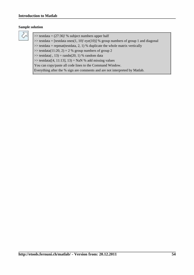
Sample solution
>> testdata = (27:36)' % subject numbers upper half>> testdata = [testdata ones(1, 10)' eye(10)] % group numbers of group 1 and diagonal>> testdata = repmat(testdata, 2, 1) % duplicate the whole matrix vertically>> testdata(11:20, 2) = 2 % group numbers of group 2>> testdata(:, 13) = randn(20, 1) % random data>> testdata([4, 11:13], 13) = NaN % add missing valuesYou can copy/paste all code lines to the Command Window.Everything after the % sign are comments and are not interpreted by Matlab.
Introduction to Matlab
http://etools.fernuni.ch/matlab/ - Version from: 20.12.2011 55
Summary
Points to remember
• A semicolon after a command suppresses the output of the created values in theCommand Window.
• Matrices can be concatenated horizontally and vertically by means of the normal[ ]-notation. Instead of single numerical values, complete matrices are used,e.g. d = [a; b]. The to-be-concatenated matrices need to have the samedimensions, that is the equal number of rows when concatenating horizontally, andequal number of columns when concatenating vertically.
Commands
• horzcat, vertcat: horizontal or vertical concatenation of matrices
• cat: general command to concatenate matrices in rows, columns, planes, etc.
• repmat: duplicate a matrix
• zeros, ones create a matrix with zeroes or ones
• rand, randn generate matrices containing random numbers with equal ornormal distribution.
• fliplr, flipud: mirrors a matrix left/right or up/down
• rot90: rotation by 90 degrees
• data': transposition of matrix data, i.e. swapping rows and columns
Introduction to Matlab
http://etools.fernuni.ch/matlab/ - Version from: 20.12.2011 56
Mathematical Operators and FunctionsIn this section, mathematical operators and functions are explained.Mathematical operators are mathematical operation symbols such as:
• addition +, subtraction -, sign, etc.
• multiplication * and division /
• exponential functions such as square ^2
• In this context, the question of priorities of operations and the bracket rules are important as well.
Other mathematical manipulations are realised as functions, e.g.
• trigonometrical functions: sine, cosine, tangent, etc.
• descriptive functions such as minimum, maximum, mean values and the like
• basic mathematical functions such as: square root, logarithm, sum, rounding, etc.
• and many more...
The range of functions provided by Matlab is enormous, thus only the most important ones can be introducedin this course.Later on, two exercises will be provided so that you can practise the use of functions and operators.
The Help System provides more information on all available functions. Call this by enteringelementary math in the search field of the Help System.
Introduction to Matlab
http://etools.fernuni.ch/matlab/ - Version from: 20.12.2011 57
Operators
The Help System provides a good overview over the mathematical operators and how to spell them.To display this information, you can either enter arithmetic operators in the Help Navigator, or youcan type docsearch 'arithmetic operators' in the Command Window (the invertedcommas are necessary because the search term includes a space).When performing calculations, certain peculiarities of Matlab become relevant. As long as you
exclusively work with scalars 4, everything works as you would expect from a pocket calculator.
However, operations with matrices (and vectors 5) follow other rules in some cases (linear algebra).
Please try to understand the following examples:
>> magic(3) + ones(3)>> a(1:3, 1:3) = 5;>> a * magic(3)>> a .* magic(3)>> magic(3) * 5
Addition is always performed element by element. The two matriceshave to be of the same size.Multiplication of two matrices is NOT performed element by element(linear algebra, usually not important for applications in our field).To perform element-by-element multiplication, you can use the operator .*(array multiplication, element-by-element product)To multiply each element of a matrix with 5, you can just multiply it with a scalar(5 in this case). This method is called «scalar expansion».
If you are unsure about the function of an operator, you can just test it in command line mode before insertingthe statement into your program.The sequence of how different operators are evaluated follows the general precedence mathematical rules(e.g. multiplication/division before addidion/subtraction ); as usual, brackets are used if a different sequenceis necessary.
You can find help on this topic by using the key word operator precedence in the Help System.
Introduction to Matlab
http://etools.fernuni.ch/matlab/ - Version from: 20.12.2011 58
Functions
Matlab provides a plethora of pre-defined mathematical functions (e.g. sine, mean, square root, etc.)
In the Help System, you find the relevant information in Contents under Function reference >Mathematics > Elementary math
Examples for mathematical functions:
>> data = magic(10);>> sum(data)>> sum(sum(data))>> min(data)>> max(data)>> std(data)>> sin(data)>> round(pi)>> why
calculates the sum in columnsfor the overall sum, two sum statements can be nestedminimum and maximum per columnstandard deviation in columnsfunctions such as the sine separately calculate the results for each elementrounding functionanother «function»: answer on all possible questions...
Introduction to Matlab
http://etools.fernuni.ch/matlab/ - Version from: 20.12.2011 59
Exercise 2: Implementing a Mathematical Formula
Try to implement the formula of the Gaussian bell shape 6.
m is the mean value or the expected (peak) value Erwartungswert (peak of the curve)s is the standard deviation ("width" of the shape)x is the independent valuee is the exponential function, in Matlab to be executed with exp. The square root function is called sqrt
>> m = 3; s = 5; x = 2;>> y = ...
definition of input valuesHow is the formula to be written correctly? The result should be 0.0782
Sample solution
>> m = 3; s = 5; x = 2;>> y = 1/(s*sqrt(2*pi))*exp(-1/2*((x-m)/s)^2)
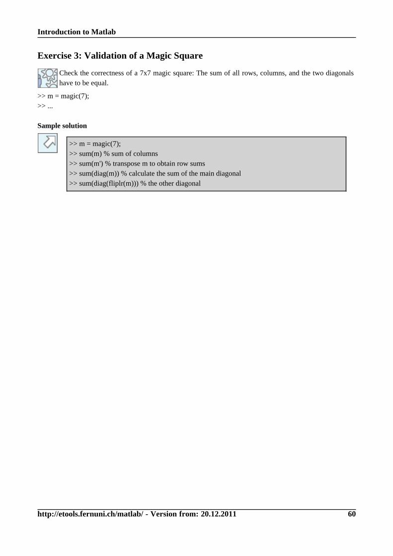
Introduction to Matlab
http://etools.fernuni.ch/matlab/ - Version from: 20.12.2011 60
Exercise 3: Validation of a Magic Square
Check the correctness of a 7x7 magic square: The sum of all rows, columns, and the two diagonalshave to be equal.
>> m = magic(7);>> ...
Sample solution
>> m = magic(7);>> sum(m) % sum of columns>> sum(m') % transpose m to obtain row sums>> sum(diag(m)) % calculate the sum of the main diagonal>> sum(diag(fliplr(m))) % the other diagonal
Introduction to Matlab
http://etools.fernuni.ch/matlab/ - Version from: 20.12.2011 61
Summary
Points to remember
• When evaluating consecutive mathematical operations, the sequence of how theyare performed follows the general mathematical rules (e.g. multiplication/divisionbefore addition/subtraction). As usual, brackets are needed if a different sequenceis necessary.
• You can find an overview of all operators by typing docsearch 'arithmetic operators'
• Addition and subtraction of whole matrices is performed element-by-element.
• Element-by-element mulitplication and division of whole matrices requires aspecial syntax: a .* b and a ./ b.Otherwise, Matlab will perform a matrix multiplication or division according tothe rules of linear algebra, which are different (and which are seldom relevant forapplications in psychology).
• Help System: You find the function overview in «Contents» Function reference> Mathematics > Elementary math.
Commands
• sum: calculates the sum
• min, max: minimum and maximum
• std: standard deviation
• sin, cos, tan etc.: trigonometric functions
• round: rounding
Introduction to Matlab
http://etools.fernuni.ch/matlab/ - Version from: 20.12.2011 62
Self-test QuestionsTo test your understanding, please try to answer the questions below.
User interfaceWhich command is used to clear the command window?
❍ clear
❍ clc
❍ home
❍ clrcmd
What is NOT possible to do in the Workspace window?
❍ Remove variables from the Workspace
❍ Change the contents of variables
❍ Read data from external sources
❍ perform calculations
How can you select the folders in which Matlab searches for functions (M-files)?
❍ In the Current Directory browser
❍ with cd (change directory)
❍ By using the menu item File > Set Path
Help SystemIn the Help System, try to find the answer to the following question:The function to draw a three-dimensional scatter plot is ___________ .
MatricesWhich statement will generate the matrix a shown below?
❍ a = [ 1 5 8 3, 6 6 7 1, 0 1 0 8]
❍ a = [ 1 5 8 3; 6 6 7 1; 0 1 0 8]
❍ a = ( 1 5 8 3; 6 6 7 1; 0 1 0 8)
❍ a = [ 1 6 0; 5 6 1; 8 7 0; 3 1 8 ]
Which command sequence leads to the pictured matrix being printed in the Command Window?
❍ a=[0 8 3;3 5 5]; b=a'; b(1,:)=NaN; [a b]
❍ a=[0 8 3;3 5 5]; b=transpond(a); b(1,:)=[]; [a b]
Introduction to Matlab
http://etools.fernuni.ch/matlab/ - Version from: 20.12.2011 63
❍ a=[0 8 3;3 5 5]; b=a'; b(1,:)=[]; [a b]
❍ a=[0 8 3;3 5 5]; b=a'; b=b(2:3,:); [a; b]
Mathematical operationsWhich code represents the shown formula?
❍ y = 2*exp(-t/tau)/sqrt(x+1*x-1)
❍ y = 2*exp(-t/tau)/sqrt((x+1)*(x-1))
❍ y = 2(exp(-t/tau)/sqrt((x+1)*(x-1)))
❍ y = 2*e^(-t/tau)/sqrt((x+1)*(x-1))
Introduction to Matlab
http://etools.fernuni.ch/matlab/ - Version from: 20.12.2011 64
GlossaryEEG:
Electro-encephalography: registration of the electrical activity of the brainfMRI:
functional magnetic resonance imagingGaussian bell shape:
density function of normally distributed datamatrix:
The most important way to represent data in Matlab. In the field of mathematics, a matrix is a table ofnumbers or other values. Matrices differ from ordinary tables in that they can be used for calculations.Usually, the expression «matrix» refers to two- or higher-dimensional matrices (cf. scalar, vector).
scalar:«null-dimensional» matrix, i.e. only one element
vector:one-dimensional matrix, that is only one row or one column
Introduction to Matlab
http://etools.fernuni.ch/matlab/ - Version from: 20.12.2011 65
Lesson 2: Programming in MatlabBasically, a program is a sequence of statements that will be executed when running the program. Thesuccession of executed statements is determined by program control structures such as loops or conditionalbranchings. This sequence of statements is stored in a file and can thus be called again at any time.
Learning Objectives
• You know the most important functions of the Editor.
• You understand the difference between scripts and functions.
• You can write simple scripts and functions.
• You know the most important loop and branching structures.
• You know how to use character strings.
Introduction to Matlab
http://etools.fernuni.ch/matlab/ - Version from: 20.12.2011 66
M-Files: Scripts and FunctionsAll programs written in Matlab are stored as so-called M-files with the file name extension .m. This is alsotrue for most functions that are included in Matlab's basic function library as well as additional toolboxes. Inthe following sections, you will learn how to write and execute such programs.There are two kinds of program or M-files: scripts and functions.
ScriptsA script contains a sequence of statements that works in the same way as if you entered these statements oneafter the other in the Command Window. Accordingly, scripts can access all variables in the Workspace, andvariables created by scripts are stored in the Workspace.
FunctionsA function is characterised by the fact that (in most cases) values are passed to it to be processed, and thefunction returns the calculated results to the «caller» (i.e. to the statement entered in the Command Window, oranother script or function). Thus, this is the same as - for instance - with standard functions, e.g. computationof a mean value with a = mean(b). The data to be processed are passed to the function in matrix b, andthe calculated mean value is returned in variable a.
The Editor/DebuggerAs a prerequisite for being able to write scripts and functions, you have to get to know the proper tool, that isthe Editor. It is designed to edit M-files. This will be explained in the next section.At the same time, this program serves as the so-called «Debugger», that is the aid to find errors (bugs)in a program and fix them (referred to as debugging). This will be introduced later in Lesson 3, SectionApplications: External Files.
Introduction to Matlab
http://etools.fernuni.ch/matlab/ - Version from: 20.12.2011 67
The Editor/Debugger
To write programs, the built-in Editor is used. The Editor also serves as Debugger, i.e. the tool to supporttracking down errors.
The Debugger will be demonstrated in Lesson 3 in the Example: Data Import.
The editor can be called in different ways:
• By typing edit or edit function name (or script name)
• by selecting a function or script name in the Command Window and choosing open via the context menu(right mouse click, or ctrl-click on a Mac with single-button mouse)
• or by doing the same in the Directory Browser.
Please note: In some older Matlab versions, if you double click an M-file (that is, a Matlab programfile with the file name extension .m) in the Windows file manager, the Matlab Editor is activated aswell, but without the Debugging features.
Demonstration of the editor: Please perform the steps described below to see how programs arewritten in the editor.
• Start the editor by typing edit in the Command Window. While opening, the editor creates an emptyM-file.
• Copy-and-paste the following statements to the Editor window.
[X,Y,Z] = peaks(30);surfc(X,Y,Z)colormap hsvaxis([-3 3 -3 3 -10 5])
• Save the program by selecting File > Save as...; name it editordemo.m. You should save it to the locationyou have defined earlier as the path for your M-files (see Configuration of Matlab).
• In the Command Window, type editordemo; now the program is executed.
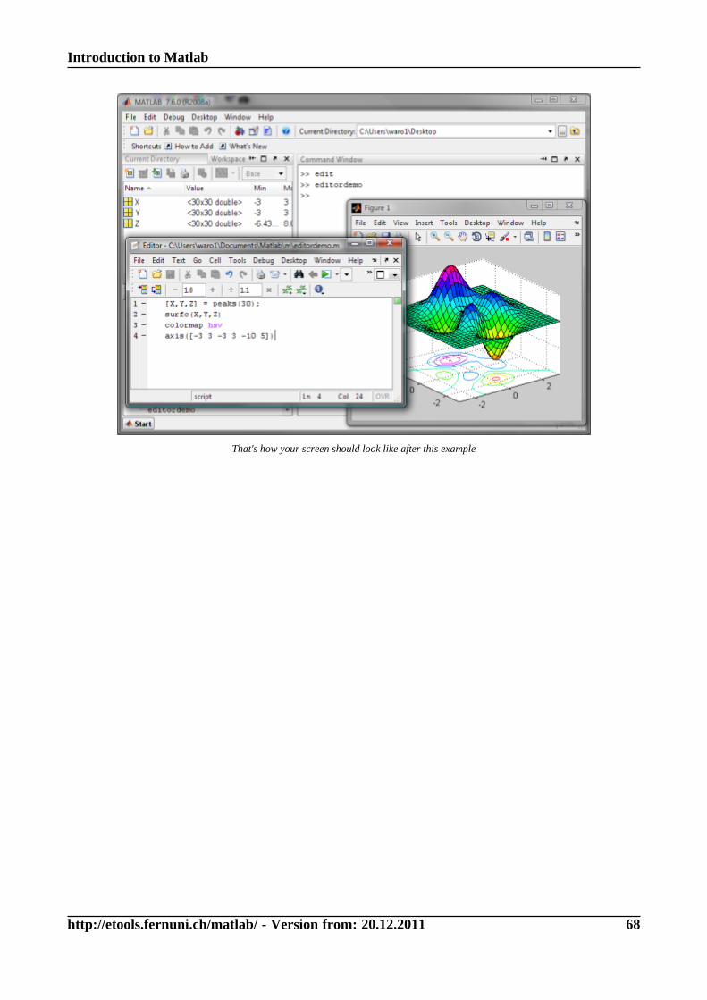
Introduction to Matlab
http://etools.fernuni.ch/matlab/ - Version from: 20.12.2011 68
That's how your screen should look like after this example
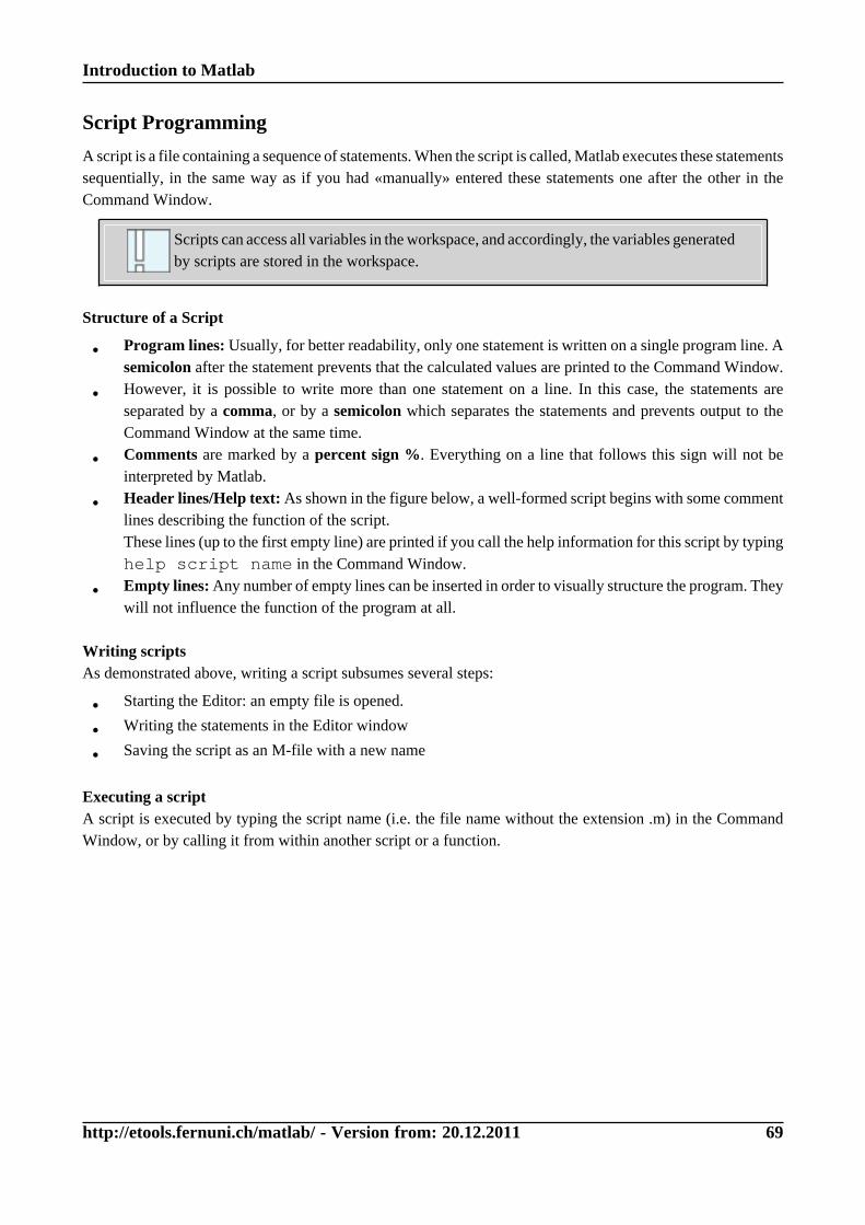
Introduction to Matlab
http://etools.fernuni.ch/matlab/ - Version from: 20.12.2011 69
Script Programming
A script is a file containing a sequence of statements. When the script is called, Matlab executes these statementssequentially, in the same way as if you had «manually» entered these statements one after the other in theCommand Window.
Scripts can access all variables in the workspace, and accordingly, the variables generatedby scripts are stored in the workspace.
Structure of a Script
• Program lines: Usually, for better readability, only one statement is written on a single program line. Asemicolon after the statement prevents that the calculated values are printed to the Command Window.
• However, it is possible to write more than one statement on a line. In this case, the statements areseparated by a comma, or by a semicolon which separates the statements and prevents output to theCommand Window at the same time.
• Comments are marked by a percent sign %. Everything on a line that follows this sign will not beinterpreted by Matlab.
• Header lines/Help text: As shown in the figure below, a well-formed script begins with some commentlines describing the function of the script.These lines (up to the first empty line) are printed if you call the help information for this script by typinghelp script name in the Command Window.
• Empty lines: Any number of empty lines can be inserted in order to visually structure the program. Theywill not influence the function of the program at all.
Writing scriptsAs demonstrated above, writing a script subsumes several steps:
• Starting the Editor: an empty file is opened.
• Writing the statements in the Editor window
• Saving the script as an M-file with a new name
Executing a scriptA script is executed by typing the script name (i.e. the file name without the extension .m) in the CommandWindow, or by calling it from within another script or a function.
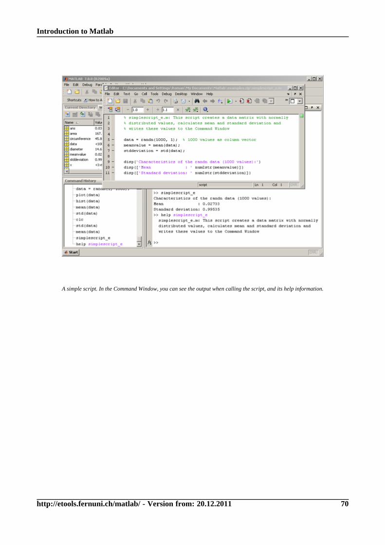
Introduction to Matlab
http://etools.fernuni.ch/matlab/ - Version from: 20.12.2011 70
A simple script. In the Command Window, you can see the output when calling the script, and its help information.
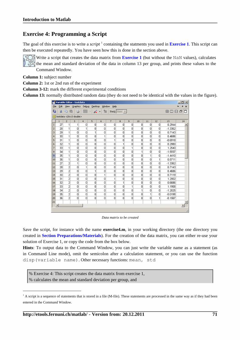
Introduction to Matlab
http://etools.fernuni.ch/matlab/ - Version from: 20.12.2011 71
Exercise 4: Programming a Script
The goal of this exercise is to write a script 1 containing the statments you used in Exercise 1. This script canthen be executed repeatedly. You have seen how this is done in the section above.
Write a script that creates the data matrix from Exercise 1 (but without the NaN values), calculatesthe mean and standard deviation of the data in column 13 per group, and prints these values to theCommand Window.
Column 1: subject numberColumn 2: 1st or 2nd run of the experimentColumn 3-12: mark the different experimental conditionsColumn 13: normally distributed random data (they do not need to be identical with the values in the figure).
Data matrix to be created
Save the script, for instance with the name exercise4.m, in your working directory (the one directory youcreated in Section Preparations/Materials). For the creation of the data matrix, you can either re-use yoursolution of Exercise 1, or copy the code from the box below.Hints: To output data to the Command Window, you can just write the variable name as a statement (asin Command Line mode), omit the semicolon after a calculation statement, or you can use the functiondisp(variable name). Other necessary functions: mean, std
% Exercise 4: This script creates the data matrix from exercise 1,% calculates the mean and standard deviation per group, and
1 A script is a sequence of statements that is stored in a file (M-file). These statements are processed in the same way as if they had been
entered in the Command Window.
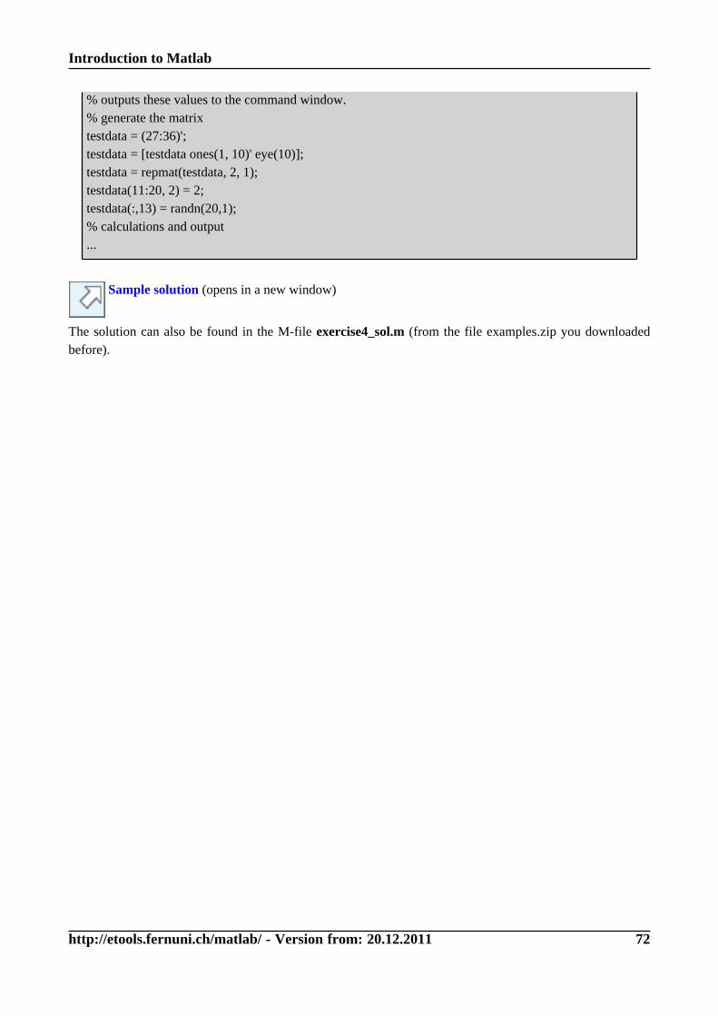
Introduction to Matlab
http://etools.fernuni.ch/matlab/ - Version from: 20.12.2011 72
% outputs these values to the command window.% generate the matrixtestdata = (27:36)';testdata = [testdata ones(1, 10)' eye(10)];testdata = repmat(testdata, 2, 1);testdata(11:20, 2) = 2;testdata(:,13) = randn(20,1);% calculations and output...
Sample solution (opens in a new window)
The solution can also be found in the M-file exercise4_sol.m (from the file examples.zip you downloadedbefore).
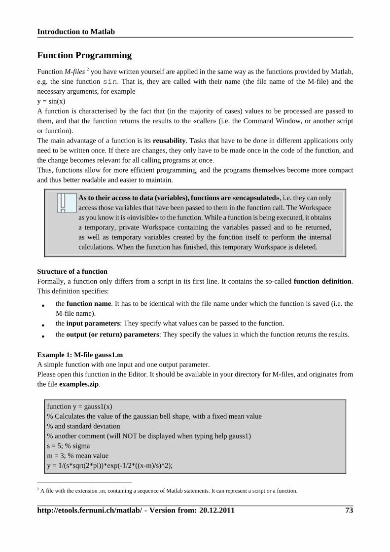
Introduction to Matlab
http://etools.fernuni.ch/matlab/ - Version from: 20.12.2011 73
Function Programming
Function M-files 2 you have written yourself are applied in the same way as the functions provided by Matlab,e.g. the sine function sin. That is, they are called with their name (the file name of the M-file) and thenecessary arguments, for exampley = sin(x)A function is characterised by the fact that (in the majority of cases) values to be processed are passed tothem, and that the function returns the results to the «caller» (i.e. the Command Window, or another scriptor function).The main advantage of a function is its reusability. Tasks that have to be done in different applications onlyneed to be written once. If there are changes, they only have to be made once in the code of the function, andthe change becomes relevant for all calling programs at once.Thus, functions allow for more efficient programming, and the programs themselves become more compactand thus better readable and easier to maintain.
As to their access to data (variables), functions are «encapsulated», i.e. they can onlyaccess those variables that have been passed to them in the function call. The Workspaceas you know it is «invisible» to the function. While a function is being executed, it obtainsa temporary, private Workspace containing the variables passed and to be returned,as well as temporary variables created by the function itself to perform the internalcalculations. When the function has finished, this temporary Workspace is deleted.
Structure of a functionFormally, a function only differs from a script in its first line. It contains the so-called function definition.This definition specifies:
• the function name. It has to be identical with the file name under which the function is saved (i.e. theM-file name).
• the input parameters: They specify what values can be passed to the function.
• the output (or return) parameters: They specify the values in which the function returns the results.
Example 1: M-file gauss1.mA simple function with one input and one output parameter.Please open this function in the Editor. It should be available in your directory for M-files, and originates fromthe file examples.zip.
function y = gauss1(x)% Calculates the value of the gaussian bell shape, with a fixed mean value% and standard deviation% another comment (will NOT be displayed when typing help gauss1)s = 5; % sigmam = 3; % mean valuey = 1/(s*sqrt(2*pi))*exp(-1/2*((x-m)/s)^2);
2 A file with the extension .m, containing a sequence of Matlab statements. It can represent a script or a function.
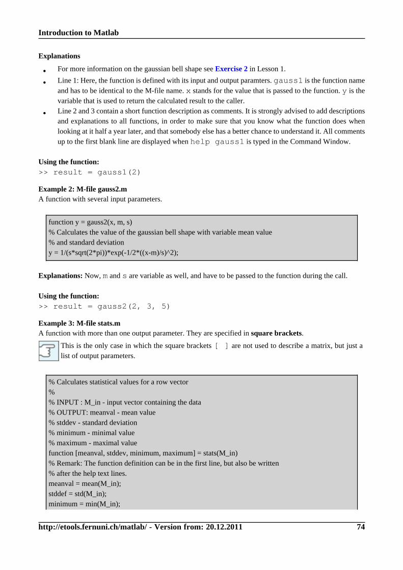
Introduction to Matlab
http://etools.fernuni.ch/matlab/ - Version from: 20.12.2011 74
Explanations
• For more information on the gaussian bell shape see Exercise 2 in Lesson 1.
• Line 1: Here, the function is defined with its input and output paramters. gauss1 is the function nameand has to be identical to the M-file name. x stands for the value that is passed to the function. y is thevariable that is used to return the calculated result to the caller.
• Line 2 and 3 contain a short function description as comments. It is strongly advised to add descriptionsand explanations to all functions, in order to make sure that you know what the function does whenlooking at it half a year later, and that somebody else has a better chance to understand it. All commentsup to the first blank line are displayed when help gauss1 is typed in the Command Window.
Using the function:>> result = gauss1(2)
Example 2: M-file gauss2.mA function with several input parameters.
function y = gauss2(x, m, s)% Calculates the value of the gaussian bell shape with variable mean value% and standard deviationy = 1/(s*sqrt(2*pi))*exp(-1/2*((x-m)/s)^2);
Explanations: Now, m and s are variable as well, and have to be passed to the function during the call.
Using the function:>> result = gauss2(2, 3, 5)
Example 3: M-file stats.mA function with more than one output parameter. They are specified in square brackets.
This is the only case in which the square brackets [ ] are not used to describe a matrix, but just alist of output parameters.
% Calculates statistical values for a row vector%% INPUT : M_in - input vector containing the data% OUTPUT: meanval - mean value% stddev - standard deviation% minimum - minimal value% maximum - maximal valuefunction [meanval, stddev, minimum, maximum] = stats(M_in)% Remark: The function definition can be in the first line, but also be written% after the help text lines.meanval = mean(M_in);stddef = std(M_in);minimum = min(M_in);
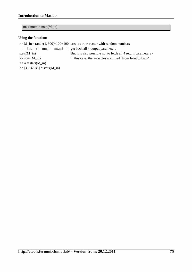
Introduction to Matlab
http://etools.fernuni.ch/matlab/ - Version from: 20.12.2011 75
maximum = max(M_in);
Using the function:
>> M_in = randn(1, 300)*100+100>> [m, s, mnm, mxm] =stats(M_in)>> stats(M_in)>> a = stats(M_in)>> [s1, s2, s3] = stats(M_in)
create a row vector with random numbersget back all 4 output parametersBut it is also possible not to fetch all 4 return parameters -in this case, the variables are filled "from front to back".
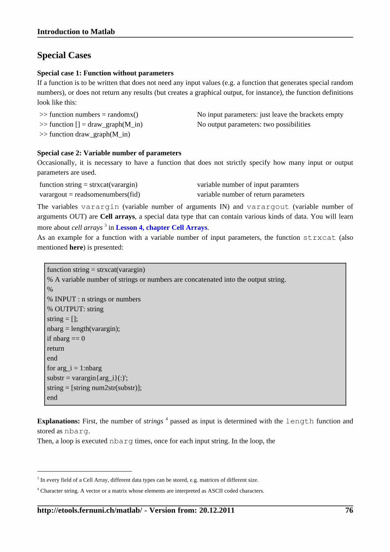
Introduction to Matlab
http://etools.fernuni.ch/matlab/ - Version from: 20.12.2011 76
Special Cases
Special case 1: Function without parametersIf a function is to be written that does not need any input values (e.g. a function that generates special randomnumbers), or does not return any results (but creates a graphical output, for instance), the function definitionslook like this:
>> function numbers = randomx()>> function [] = draw_graph(M_in)>> function draw_graph(M_in)
No input parameters: just leave the brackets emptyNo output parameters: two possibilities
Special case 2: Variable number of parametersOccasionally, it is necessary to have a function that does not strictly specify how many input or outputparameters are used.
function string = strxcat(varargin)varargout = readsomenumbers(fid)
variable number of input paramtersvariable number of return parameters
The variables varargin (variable number of arguments IN) and varargout (variable number ofarguments OUT) are Cell arrays, a special data type that can contain various kinds of data. You will learn
more about cell arrays 3 in Lesson 4, chapter Cell Arrays.As an example for a function with a variable number of input parameters, the function strxcat (alsomentioned here) is presented:
function string = strxcat(varargin)% A variable number of strings or numbers are concatenated into the output string.%% INPUT : n strings or numbers% OUTPUT: stringstring = [];nbarg = length(varargin);if nbarg == 0returnendfor arg_i = 1:nbargsubstr = varargin{arg_i}(:)';string = [string num2str(substr)];end
Explanations: First, the number of strings 4 passed as input is determined with the length function andstored as nbarg.Then, a loop is executed nbarg times, once for each input string. In the loop, the
3 In every field of a Cell Array, different data types can be stored, e.g. matrices of different size.
4 Character string. A vector or a matrix whose elements are interpreted as ASCII coded characters.
Introduction to Matlab
http://etools.fernuni.ch/matlab/ - Version from: 20.12.2011 77
arg_i-th element is extracted, converted from number into string if necessary, and concatenated with theprevious strings.
Introduction to Matlab
http://etools.fernuni.ch/matlab/ - Version from: 20.12.2011 78
Summary
Points to remember
• A script contains a sequence of statements that are processed in the same way asif they had been entered one after the other in the Command Window.
• A script can be called from the Command Window by typing its file name(without .m). In the same way, a script can be called from within another scriptor function.
• Scripts can access all variables in the Workspace, and the variables created in thescript are stored in the Workspace.
• A function differes from a script in that (in most cases) values are passed to thefunction to be processed, and the results can be passed back to the «caller».
• Contrary to scripts, functions are «encapsulated» with regard to data access, i.e.they cannot access the variables in the general Workspace, but only those variablesthat have been passed in the function call.During execution, a function obtains a temporary, private Workspace, containigthe variables passed as input and return parameters as well as variables definedwithin the function itself.
• A semicolon at the end of a code line prevents the output of calculated or createdvalues in the Command Window.
Commands
• function [return parameters] = function name(variables for input parameters)definition of a function with input and return parameters
• disp(): output of values to the Command Window
Introduction to Matlab
http://etools.fernuni.ch/matlab/ - Version from: 20.12.2011 79
Program Control Structures: LoopsIt is often necessary to repeat a sequence of statements. This is achieved by using loops. There are two kindsof loops:
• the for-loop: It is used if it is pre-determined how many times the statements have to be repeated.
• the while-loop: It allows for making the number of repetitions dependent on a comparison within theloop.
Introduction to Matlab
http://etools.fernuni.ch/matlab/ - Version from: 20.12.2011 80
The For Loop
If the number of necessary repetitions is known before the loop is started, the for loopis applied.
This is the schematic syntax of the for loop:for indexvar = rangestatement 1...statement nendindexvar - the so-called loop index. With every pass through the loop, it is set to the next value of range.It can be used like any other variable within the loop. Any valid variable name is allowed.range - row vector or matrix. It defines which values are assigned to indexvar.
For loop examples
Please try to understand the way how for loops work by studying the examples below.
Simple for loop:
>> for index = 1:30>> facts = factor(index);>> disp(facts)>> sumvalue = sum(facts);>> end
Matlab does not do anything until it hits endcalculate the prime factors of the loop indexdisplay themfurther statementswith this, the loop is closed, and will be executed
Basically, for the loop index, all notations of vectors are allowed:
>> for i = pi:-.3:-pi, i, end>> for i = [1 4 7 11 13 17 3 5], i, end>> for i = rand(1,10) * 20, i, end
any sequence of numbersenumerationvector created by a function, but only row vectors
If a matrix is given as range, the loop index obtains a whole column of range at each pass. That is, theloop is executed as many times as there are columns in the matrix.>> for i = magic(7), i, end
Introduction to Matlab
http://etools.fernuni.ch/matlab/ - Version from: 20.12.2011 81
The While Loop
The while loop is applied when the number of passes is dependent on a comparison madeeach time the loop is executed, usually at the begin of the loop.
The syntax of the while loop in pseudo code:while conditionstatement 1...statement nendThe loop is executed as long as the condition results in true (i.e. a value > 0). The condition is alwaysevaluated at the begin of the loop. The first time the condition evaluates as false (value = 0), the loop is left.Program execution then continues with the first statement after the loop (i.e. the corresponding end statement).You will find detailed information on how to specify comparisons in the section Comparison Operators andLogical Operations.
A simple while loop:
>> index = 1;>> while index <= 30>> disp(factor(index))>> index = index + 1;>> end
execute the loop as long as index is smaller as or equal to 30print prime factorsincrement index
Introduction to Matlab
http://etools.fernuni.ch/matlab/ - Version from: 20.12.2011 82
Exit Loops with the break Statement
It is possible to prematurely exit for- and while loops by means of the break statement, even if it has not«finished». That is, the break statement causes the program execution to continue after the end statementthat closes the loop.With this statement, for instance, a while loop can be written whose exit comparison is done at the end oranywhere within the loop instead of at the beginning. Or you can terminate a for loop before the loop indexhas reached its last value.
Example 1: for loop with premature exit
>> for index = 1:30>> disp(sum(factor(index)))>> if index == 20, break, end>> end
already leave the loop when the index is 20
Example 2: while loop with breakindex = 1;while truedisp(factor(index))if index > 30breakendindex = index + 1;endExplanationstrue (or the value 1) in the while statement means: the comparison result is true, in this example: ALWAYS(counterpart: false or 0).
Introduction to Matlab
http://etools.fernuni.ch/matlab/ - Version from: 20.12.2011 83
Exercise 5: Gaussian function for a vector
Rewrite the Gaussian function version 2 (M-file gauss2.m) by means of a loop in order to enable it tocalculate the values for a row vector and return the results as a vector. Save the function as gauss3.m).Start out with these lines:
function Moutput = gauss3(Minput, m, s)% Calculates the values of the gaussian bell shape for the row vector% Minput, with the mean value m and standard deviation s...Afterwards call the function with values from -5 to 5 (with intervals of 0.1) and graphically display the valuesby means of plot
Sample solution (opens in a new window)
The solution can also be found in the M-file gauss3_sol.m
Introduction to Matlab
http://etools.fernuni.ch/matlab/ - Version from: 20.12.2011 84
Vectorisation of Loops
Thanks to the data representation method as matrices, it is often possible to process complete data sets muchmore efficiently than as it would be feasible with loops.
Please have a look at the following example:
The task is to compute the sine of 1001 values from 0 to 10 and store it in row vector y. Using the means youknow up to now, one possibility to solve this task is:>> i = 0;>> for t = 0:.01:10>> i = i + 1;>> y(i) = sin(t);>> endThe «vectorised» version is simpler and executes faster:>> t = 0:.01:10;>> y = sin(t);Or in an even more compact form:>> y = sin(0:.01:10);
Introduction to Matlab
http://etools.fernuni.ch/matlab/ - Version from: 20.12.2011 85
Summary
Points to remember
• The for loop is used whenever it is predetermined how many times a sequence ofstatements has to be executed.
• The while loop is applied when the number of reiterations has to be dependenton a condition.
Commands
• for index=1:n(some statements)endRepetition loop. Instead of 1:n, any vector can be used.
• while (condition)(some statements)endLoop with conditional exit. The statements are executed as long as the conditionis fulfilled, i.e. results in true (value > 0). The comparison is always evaluated atthe beginning of the loop.
• break: allows to exit for and while loops at any time.
Introduction to Matlab
http://etools.fernuni.ch/matlab/ - Version from: 20.12.2011 86
Program Control Structures: Conditional BranchingIn almost every program it is necessary to process some statements only under certain conditions. To realisethis, so-called conditional branchings are used.Matlab offers two constructs to achieve this:
• the if-elseif-else structure, and
• the switch-case structure.
Introduction to Matlab
http://etools.fernuni.ch/matlab/ - Version from: 20.12.2011 87
The branching structure if-elseif-else
You can see how this structure works in the examples below.
Example 1: if-else structure with two cases
Load the M-file example_if.m into the Editor. You can execute the script by hitting the F5 key in the Editorwindow, or by typing example_if in the Command window.% Example 1 for if-elsea = rand(20) * 100 - 20; % generate random numbersfor i = 1:length(a)if a(i) < 0disp([num2str(a(i)) ': number is below zero'])elsedisp([num2str(a(i)) ': number is above zero'])endendExplanations: The composed statement after disp displays the current entsprechende number together withthe text. The function num2str will be explained later (see here).
Example 2: if-else structure with more than two cases
Again, you can load the appropriate M-file example_if_elseif.m into the Editor.% Example 2 for if-elseif-elsea = rand(20) * 100 - 20;for i = 1:length(a)if a(i) < 0disp([num2str(a(i)) ': number is below zero'])elseif a(i) >= 0 && a(i) <= 20 % is the value >= 0 AND <= 20?disp([num2str(a(i)) ': small number'])elsedisp([num2str(a(i)) ': large number'])endendExplanations: Obviously, it is possible to realise any number of subsequent elseif comparisons.
Introduction to Matlab
http://etools.fernuni.ch/matlab/ - Version from: 20.12.2011 88
The switch-case structure
If, in the course of a if-elseif-else structure, a great number of single comparisons with the same variable haveto be done, the switch-case structure is the better solution:The schematic syntax is:switch indicatorcase exprstatement, ..., statementcase {expr1, expr2, expr3, ...}statement, ..., statementotherwisestatement, ..., statementendindicator is the variable that contains the value on which the conditional branching is based. It can bea scalar or a string.The case statement compares the indicator with expr. If they are the same, the following statementswithin the case block are executed. Afterwards, the program is continued after the end statement.expr contains the comparison values (scalars or strings). Single values as well as Cell Arrays with severalvalues can be used.After otherwise, those statements follow that have to be executed in case none of the previous conditionshave been met.
Example: Replacing a multiple if comparison by a switch-case structurePlease study the following implementation of a multiple comparison with if-elseif-else (the function strcmpcompares two strings):if strcmp(designator,'date')% statements...elseif strcmp(designator,'start')% statements...elseif strcmp(designator,'endtrial')% statements...elseif strcmp(designator,'fix') || strcmp(designator,'sacc') || strcmp(designator,'blink')% statements...else% all remaining casesendThe following implementation is more elegant and easier to understand:switch designatorcase 'date'% statements...case 'starttrial'% statements...case 'endtrial'% statements...case {'fix', 'sacc', 'blink'}

Introduction to Matlab
http://etools.fernuni.ch/matlab/ - Version from: 20.12.2011 89
% statements...otherwise% all remaining casesend
Introduction to Matlab
http://etools.fernuni.ch/matlab/ - Version from: 20.12.2011 90
Comparison Operators and Logical Operations
In the two examples above, you have already seen various comparison operators such as «smaller than» oder«larger than or equal as».
Comparison OperatorsBelow, the basic comparisons are shown:
A == BA ~= BA < B or A > BA <= B or A >= B
test for equality: double equal sign!not to be mixed up with =, that would be a value assignmenttest for inequality. The tilde symbol ~ always means alogical inversion, that is, NOTtest for «smaller» or «larger»test for «smaller or equal» or «larger or equal»
As the result, comparison operation either return the value true (internally pre-defined as 1, but any value >0 is interpreted as "true") oder false (internally represented as 0, zero).
For an overview, see the Help System with the key word 'relational operators'.
Concatenation of ComparisonsIt is possible to combine more than one comparison. To achieve this, two logical operators are available:
• && as AND operation: The expression is only true if condition 1 and condition 2 are true.
• || as OR operation: Contrary to common language use, it means "A or B or both"!
Examples:
>> true>> false>> x = 77; y = 12;>> x < y>> x ~= y>> x <= 77 && y > 0>> v = x == y>> ~v>> a=1:4; b=[1 3 5 7];>> length(a)==4 || ~isempty(b)>> a == b
the pre-defined valuesis x smaller than y?is x not equal to y?&& and || are always evaluated last, thus not brackets are necessaryv now contains the truth value 'false' or 0the ~ «inverts» the truth value (NOT function)Comparisons of vectors and matrices are evaluated element-by-element! This only works if both are of the same size.
Such comparisons mostly appear after an if statement, as shown in the previous section.>> if (x < y || y ~= 0) && (v == true || numel(a) == 4)>> disp('that is true')>> else>> disp('that is wrong')>> end
Introduction to Matlab
http://etools.fernuni.ch/matlab/ - Version from: 20.12.2011 91
By the way: If a program line becomes very long so that it does not fit into the editorwindow any more and thus becomes confusing, it can be split by using ...:if (x < y || y ~= 0) ...&& (v == true || numel(a) == 4)
Introduction to Matlab
http://etools.fernuni.ch/matlab/ - Version from: 20.12.2011 92
Exercise 6: Standardisation Function
Write a function named standardize, that z-standardises a maximally two-dimensional matrix ofdata (that is, it also correctly evaluates vectors, but no scalars, as at least two data points are necessaryfor these calculations).
The formula to be used is:
The function is expected to return the transformed values in a matrix with the same size as the input matrix, aswell as returning the mean value and the standard deviation. Use several for- or while loops to implement this(you might also try to figure out how a «vectorised» solution, i.e. without loops, would be realised).Before the calculation, the matrix passed to the function has to be checked for validity:
• If it is empty or only contains only one element, the function has to return an empty matrix [ ], thecalculated mean value and the standard deviation (which will then be 0 or NaN), as well as a warningtext printed to the Command Window.
• If the matrix has more than two dimensions, the function has to exit and print an appropriate errormessage.
Tips for useful functions (you might have to look them up in the Help System):mean, std, reshape, isempty, ndims, size, numel, disp, error, return
Sample solution (opens in a new window)
You can find the solution in the M-file standardize_sol.m as well; the «vectorised» solution is calledstandardize_vect.m
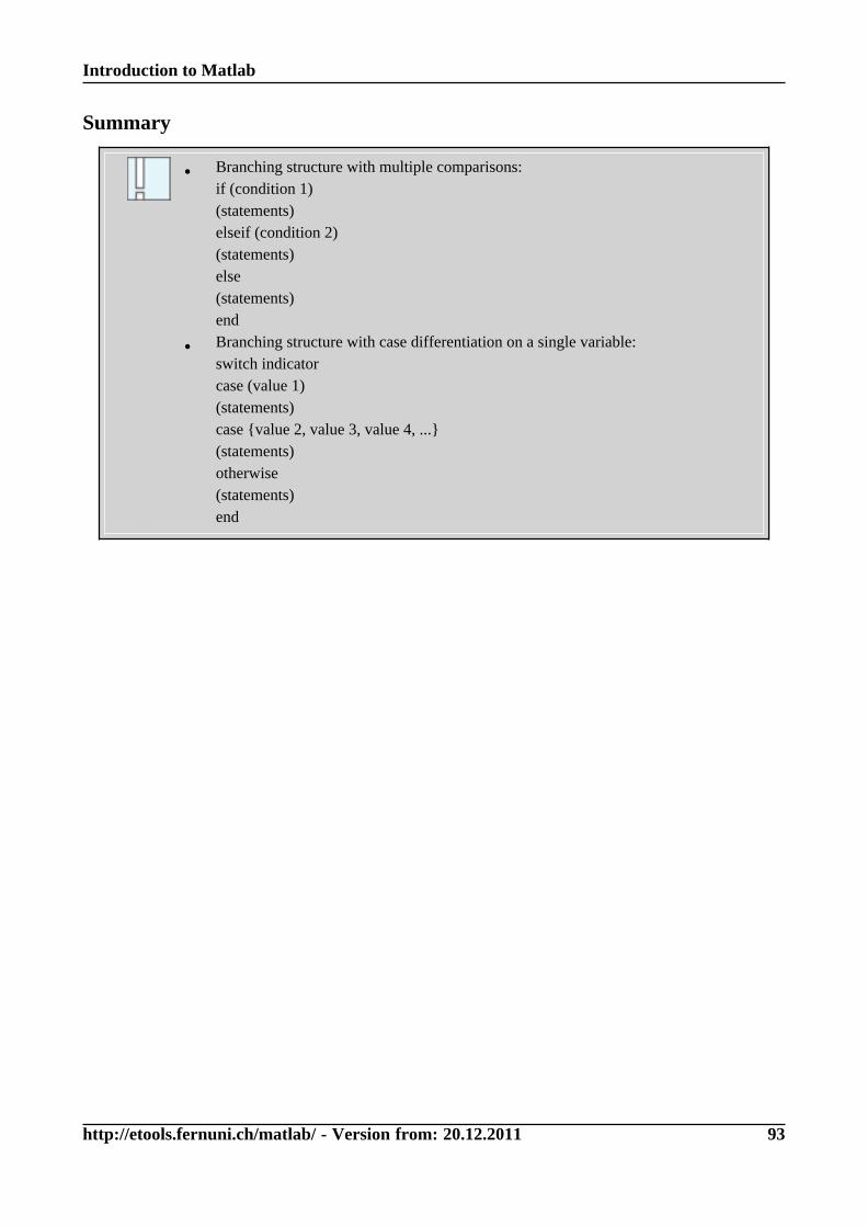
Introduction to Matlab
http://etools.fernuni.ch/matlab/ - Version from: 20.12.2011 93
Summary
• Branching structure with multiple comparisons:if (condition 1)(statements)elseif (condition 2)(statements)else(statements)end
• Branching structure with case differentiation on a single variable:switch indicatorcase (value 1)(statements)case {value 2, value 3, value 4, ...}(statements)otherwise(statements)end
Introduction to Matlab
http://etools.fernuni.ch/matlab/ - Version from: 20.12.2011 94
Data Representation 2: Character StringsUp to now, we have only worked with matrices containing numbers. However, you will often have to processtext information, that is «character strings», or short, «strings». This will be the case, for example, if you want
to import and process data from an ASCII 5 files (e.g. tab-separated data), or if you wish to output results orusage hints for the user in clear text.To this end, Matlab offers the option to store text information in matrices a well. In this case, every numberin a matrix is interpreted as character coded in ASCII.
This way to work with text information is often applied, but it is not the best and not the only wayto do this. However, it is introduced first for didactical reasons, as it is relatively easy to understand(cf. Lesson 3: Cell Arrays).
5 American Standard Code for Information Interchange, the most common norm to represent alphanumerical characters.
Introduction to Matlab
http://etools.fernuni.ch/matlab/ - Version from: 20.12.2011 95
String creation and concatenation
First you need to know how character strings (or briefly «strings») are created. Often, it is also necessary toconvert numerical results into a string and chain it with another string.
Please try to follow the examples below to find out how this is done.
>> t1 = 'The quick brown fox jumps '>> t2 = 'over the lazy dog.'>> n = num2str(23.28)>> ischar(t1)>> m = str2num('3.1415926')>> t3 = [t1 t2]>> t4 = strcat(t1, t2)
fixed texts are entered in inverted commasconversion of a number into a stringyields true if the matrix contains charactersconversion of a number that is stored in a stringinto a scalarconcatenation of text as with'normal' vectorsanother way. strcat = string concatenation
If you want to store several strings in a matrix (that is, in rows), there is a complication: As you know, allrows of a matrix have to contain the same number of elements. Thus, Matlab will fill up rows with shortertexts with blank characters (the function to vertically concatenate strings is called strvcat = string verticalconcatenation)!
>> z=['four';'five';'nine']>> z=['four';'five';'nine';'seven']>> z=strvcat('four','five','nine','seven')>> z1 = z(1, :)>> length(z1)>> z2 = deblank(z1), length(z2)
This works fine as all words have four charactersThis does not, as 'seven' is longercorrect statementaddress the first rowhowever, it is five characters long,a space character has been addeddeblank removes spaces at theend of a string
A helpful function: strxcatIf you want to concatenate several strings and numerical results, this quickly leads to complicated and confusingcode. To avoid this, you can use a little function specifically written for that purpose (it is not included in thestandard Matlab functions, you can find it with the downloaded examples).The function strxcat is defined as:function string = strxcat(varargin)
It concatenates any number of strings and numbers into a single string. Example:>> sumvalue = fix(sum(rand(1, 3000)))/100>> output = strxcat('The final amount is: ', sumvalue, ' Dollars')
strxcat is a simple example for a function with a variable number of input parameters (cf. SectionSpecial Cases). If you are interested in how this is done, you can have a closer look at it in the editor:edit strxcat
Introduction to Matlab
http://etools.fernuni.ch/matlab/ - Version from: 20.12.2011 96
Examine and Compare Strings
Find specific contents in stringsOften you will have to process data in differing ways, dependent on the content of a string. Thus you needoperations that allow for the examination of string contents.Two easily confused functions are available: strfind and findstr
Again, they are best demonstrated with examples. The variables from the preceding examples of thislesson should still be in the workspace.
>> findstr(t3, 'fox')>> findstr(t3, 'cat')>> pos = strfind(t3, ' ')
Finds a string in an other one.result: starting position(s) of the found matchesposition of all space characters in pos
Explanations: findstr compares two strings and checks whether the shorter one is contained in the longerone.strfind finds a pattern (the second argument) in a string (first argument). You may want to look up thesedifferences in the Help System.
String comparison
To find out whether two strings are identical, you cannot simply use the comparisonoperators == or ~= you already know; you have to use specific functions to that end.
The basic function is strcmp (string comparison). This function exists in several variants strcmpi, strncmp, strncmpi, that not only allow for a simple equality or inequality test, but also for testingonly a restricted number of characters, or ignoring uppercase/lowercase differences
To see these functions in action, please try out the following lines. The variables from the precedingexamples of this lesson should still linger in the workspace.
>> strcmp(z2, 'one')>> E = 'One';>> strcmp(z2, E)>> strcmpi(z2, E)>> strncmp(t2, 'over it', 4)
comparisonwrong, because the comparison is case-sensitiveif this is not wanted, use strcmpi(i stands for case-insensitive)only compares the first n characters (this is also possiblecase-insensitive - strncmpi)
Introduction to Matlab
http://etools.fernuni.ch/matlab/ - Version from: 20.12.2011 97
Summary
Points to remember
• (Character) Strings are matrices whose elements are interpreted as ASCII-codedcharacters.
• In contrast to variable names, literal texts are written in inverted commas: a = 'Hello'.Thus, Hello is not a variable, but a literal text.
Commands
• length: Determines the length of a string (same as with vectors)
• str2num: Transformation of a number stored in a string into a scalar
• num2str: Conversion of a number into a string
• ischar: returns true if the argument is a matrix containing characters
• strcat: string concatenation
• strvcat: vertical string concatenation
• deblank: removal of blank characters from the end of a string
• findstr, strfind: finds a string in another one
• strcmp, strcmpi: compare strings, with i: case-insensitive
• strncmp, strncmpi: compare the first n characters of strings, with i: case-insensitive
Introduction to Matlab
http://etools.fernuni.ch/matlab/ - Version from: 20.12.2011 98
Self-test QuestionsTo test your understanding, please try to answer the questions below.
ProgrammingWhich of the function definition(s) is/are correct? Multiple answers are possible.
❏ function hello()
❏ function (ciphers, number) = generate(value, modus)
❏ function [subj, name, age] = getsubject(1, 6)
❏ function [] = startprocess(grunt)
Which code lines fulfil the following goal: Output of the numbers 7 to 21 and their squared values in theCommand Window? Several answers can be correct.
❏ for i = 7:21, disp(i, i^2), end
❏ i=7;while i <22, disp(i, i^2), end
❏ i=6; while true, i=i+1, disp(i^2), if i==21, break, end, end
❏ for i = 7:28, disp(i, i^2), if i>20, break, end, end
Which is the result of the statement:4 >= sqrt(9) && ~false
❍ 3
❍ 0
❍ false
❍ 1
Which statement has to be inserted to get the result 1 (= true) in variable q?m = 'To err is human, but to really foul things up requires a computer.';q = ___________ (m(11:15), 'Human')
Introduction to Matlab
http://etools.fernuni.ch/matlab/ - Version from: 20.12.2011 99
GlossaryASCII:
American Standard Code for Information Interchange, the most common norm to represent alphanumericalcharacters.
Cell array:In every field of a Cell Array, different data types can be stored, e.g. matrices of different size.
Function:A sequence of statements that is stored in a file (M-file), similar to a script. However, values can be passed toa function, and the function returns results. Functions cannot access the variables in the common Workspace.
M-file:A file with the extension .m, containing a sequence of Matlab statements. It can represent a script or afunction.
Script:A script is a sequence of statements that is stored in a file (M-file). These statements are processed in thesame way as if they had been entered in the Command Window.
String:Character string. A vector or a matrix whose elements are interpreted as ASCII coded characters.
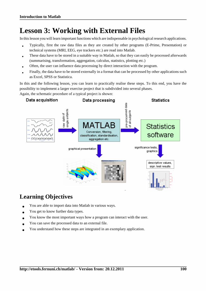
Introduction to Matlab
http://etools.fernuni.ch/matlab/ - Version from: 20.12.2011 100
Lesson 3: Working with External FilesIn this lesson you will learn important functions which are indispensable in psychological research applications.
• Typically, first the raw data files as they are created by other programs (E-Prime, Presentation) ortechnical systems (MRI, EEG, eye trackers etc.) are read into Matlab.
• These data have to be stored in a suitable way in Matlab, so that they can easily be processed afterwards(summarising, transformation, aggregation, calculus, statistics, plotting etc.)
• Often, the user can influence data processing by direct interaction with the program.
• Finally, the data have to be stored externally in a format that can be processed by other applications suchas Excel, SPSS or Statistica.
In this and the following lesson, you can learn to practically realise these steps. To this end, you have thepossibility to implement a larger exercise project that is subdivided into several phases.Again, the schematic procedure of a typical project is shown:
Learning Objectives
• You are able to import data into Matlab in various ways.
• You get to know further data types.
• You know the most important ways how a program can interact with the user.
• You can save the processed data to an external file.
• You understand how these steps are integrated in an exemplary application.
Introduction to Matlab
http://etools.fernuni.ch/matlab/ - Version from: 20.12.2011 101
Data ImportIf you want to process and visualise data, you first have to «get them into the program». Nowadays, mostsystems that are used to acquire psychophysical and behavioural data allow to store the data in simple text files.Matlab is very well equipped to import such data. Basically, there are two ways to do that:
• Comfortable features that can be used to import data «manually» from various standard applications.This option is useful to explore a single data set and graphically display the contents.
• Importing data by a Matlab program. This method is chosen if new sets of data in the same format haveto be processed again and again - that is, the typical application in research.
Introduction to Matlab
http://etools.fernuni.ch/matlab/ - Version from: 20.12.2011 102
Interactive Data Import
To quickly have a look at a data set, Matlab provides comfortable features. They let you import data from thesystem clipboard or from text, Excel, xml, or Lotus files without having to write a program for that purpose.Afterwards, the data can be processed and/or visualised.
Import by means of copy-and-pasteThis is the most simple, but not the most versatile method: Create a matrix of appropriate size in the workspace,open this matrix in the «Variable Editor» (double click on the variable name in the Workspace), and transfer
the data from applications such as Excel, SPSS or similar by means of copy-and-paste 1 or Edit > Copy andEdit > Paste).
Import from files - the «Import Wizard»
Import the file exp1.xls (it is contained in the zip file data.zip and should be found in your workingdirectory), by selecting it in the Directory Browser, and choosing «Import data» via the context menu(right click), or via File > Import Data...
As you can see, the Import Wizard creates two data sets: a matrix with the numerical data, and a «cell array» (seehere) containing the text data.You can also call the Import Wizard from within a program: uiimport (also see import)
The keyword to find information on that topic in the Help System is import wizard.
Import from the system clipboardYou can import data from the system clipboard, i.e. data that has been saved beforehand from anotherapplication by copying it to the clipboard. The following options are available; they also call the Import Wizard.
• by using Edit > Paste to Workspace...
• type uiimport -pastespecial in the Command Window
• or simply type uiimport, and select Clipboard at the item Select Data Source
1 On PC/Windows: CTRL-C and CTRL-V. On Mac OS: cmd-C and cmd-V
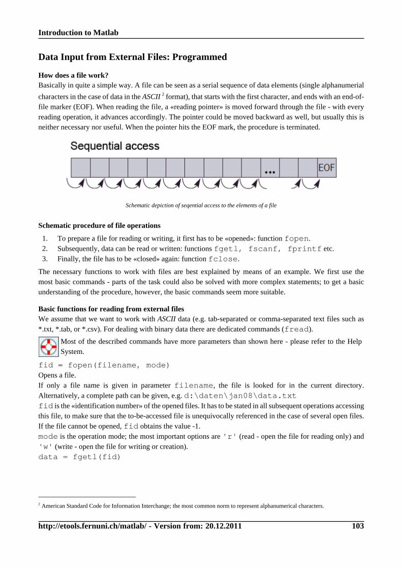
Introduction to Matlab
http://etools.fernuni.ch/matlab/ - Version from: 20.12.2011 103
Data Input from External Files: Programmed
How does a file work?Basically in quite a simple way. A file can be seen as a serial sequence of data elements (single alphanumerial
characters in the case of data in the ASCII 2 format), that starts with the first character, and ends with an end-of-file marker (EOF). When reading the file, a «reading pointer» is moved forward through the file - with everyreading operation, it advances accordingly. The pointer could be moved backward as well, but usually this isneither necessary nor useful. When the pointer hits the EOF mark, the procedure is terminated.
Schematic depiction of seqential access to the elements of a file
Schematic procedure of file operations
1. To prepare a file for reading or writing, it first has to be «opened»: function fopen.2. Subsequently, data can be read or written: functions fgetl, fscanf, fprintf etc.3. Finally, the file has to be «closed» again: function fclose.
The necessary functions to work with files are best explained by means of an example. We first use themost basic commands - parts of the task could also be solved with more complex statements; to get a basicunderstanding of the procedure, however, the basic commands seem more suitable.
Basic functions for reading from external filesWe assume that we want to work with ASCII data (e.g. tab-separated or comma-separated text files such as*.txt, *.tab, or *.csv). For dealing with binary data there are dedicated commands (fread).
Most of the described commands have more parameters than shown here - please refer to the HelpSystem.
fid = fopen(filename, mode)Opens a file.If only a file name is given in parameter filename, the file is looked for in the current directory.Alternatively, a complete path can be given, e.g. d:\daten\jan08\data.txtfid is the «identification number» of the opened files. It has to be stated in all subsequent operations accessingthis file, to make sure that the to-be-accessed file is unequivocally referenced in the case of several open files.If the file cannot be opened, fid obtains the value -1.mode is the operation mode; the most important options are 'r' (read - open the file for reading only) and'w' (write - open the file for writing or creation).data = fgetl(fid)
2 American Standard Code for Information Interchange; the most common norm to represent alphanumerical characters.
Introduction to Matlab
http://etools.fernuni.ch/matlab/ - Version from: 20.12.2011 104
Reads a complete line, that is up to the next line break (CR, LF). If the «reading pointer» is already in the middle
of the line, only the rest of the line is read. The result of the operation is a String 3 (vector 4 with characters).data = fscanf(fid, format, n)Reads n data elements in a specified format which is given in format. For the format specifications and allother options see the following example and the information in the Help System.fclose(fid)Closes the file. Only then, other application can fully access it.feof(fid)Checks whether the end of the file has been reached (eof = end of file); returns true if this is the case,otherwise false.
3 Character string. A vector or a matrix whose elements are interpreted as ASCII coded characters.
4 one-dimensional matrix, that is only one row or one column
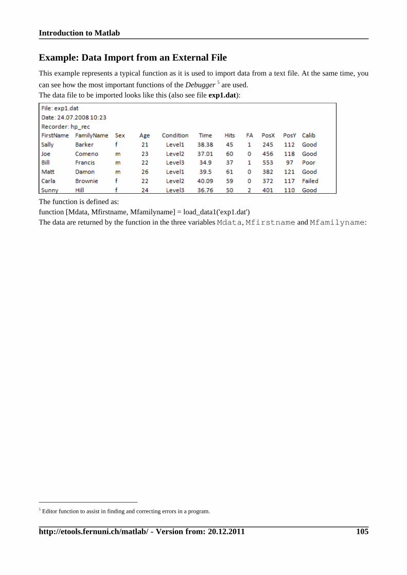
Introduction to Matlab
http://etools.fernuni.ch/matlab/ - Version from: 20.12.2011 105
Example: Data Import from an External File
This example represents a typical function as it is used to import data from a text file. At the same time, you
can see how the most important functions of the Debugger 5 are used.The data file to be imported looks like this (also see file exp1.dat):
The function is defined as:function [Mdata, Mfirstname, Mfamilyname] = load_data1('exp1.dat')The data are returned by the function in the three variables Mdata, Mfirstname and Mfamilyname:
5 Editor function to assist in finding and correcting errors in a program.
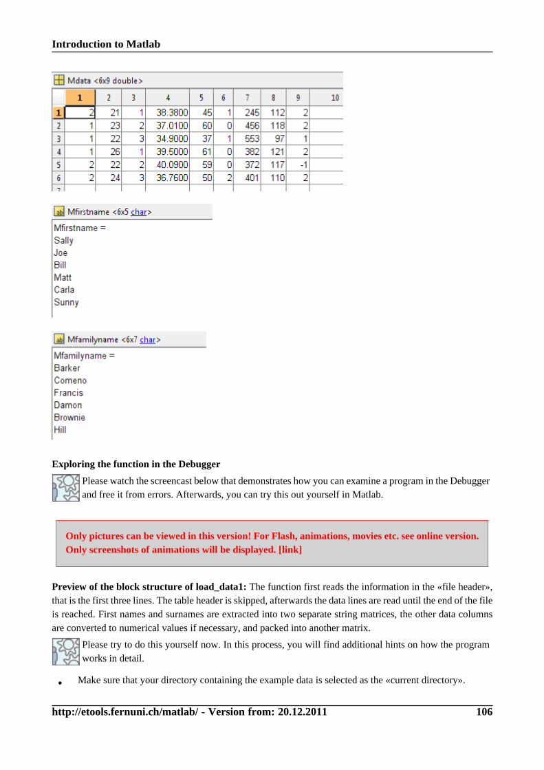
Introduction to Matlab
http://etools.fernuni.ch/matlab/ - Version from: 20.12.2011 106
Exploring the function in the Debugger
Please watch the screencast below that demonstrates how you can examine a program in the Debuggerand free it from errors. Afterwards, you can try this out yourself in Matlab.
Only pictures can be viewed in this version! For Flash, animations, movies etc. see online version.Only screenshots of animations will be displayed. [link]
Preview of the block structure of load_data1: The function first reads the information in the «file header»,that is the first three lines. The table header is skipped, afterwards the data lines are read until the end of the fileis reached. First names and surnames are extracted into two separate string matrices, the other data columnsare converted to numerical values if necessary, and packed into another matrix.
Please try to do this yourself now. In this process, you will find additional hints on how the programworks in detail.
• Make sure that your directory containing the example data is selected as the «current directory».
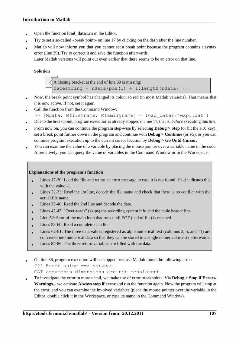
Introduction to Matlab
http://etools.fernuni.ch/matlab/ - Version from: 20.12.2011 107
• Open the function load_data1.m in the Editor.
• Try to set a so-called «break point» on line 17 by clicking on the dash after the line number.
• Matlab will now inform you that you cannot set a break point because the program contains a syntaxerror (line 39). Try to correct it and save the function afterwards.Later Matlab versions will point out even earlier that there seems to be an error on that line.
Solution
A closing bracket at the end of line 39 is missing:datestring = rdata(pos(1) + 1:length(rdata) );
• Now, the break point symbol has changed its colour to red (in most Matlab versions). That means thatit is now active. If not, set it again.
• Call the function from the Command Window:>> [Mdata, Mfirstname, Mfamilyname] = load_data1('exp1.dat')
• Due to the break point, program execution is already stopped on line 17, that is, before executing this line.
• From now on, you can continue the program step-wise by selecting Debug > Step (or hit the F10 key),set a break point further down in the program and continue with Debug > Continue (or F5), or you cancontinue program execution up to the current cursor location by Debug > Go Until Cursor.
• You can examine the value of a variable by placing the mouse pointer over a variable name in the code.Alternatively, you can query the value of variables in the Command Window or in the Workspace.
Explanations of the program's function
• Lines 17-20: Load the file and return an error message in case it is not found. fid indicates thiswith the value -1.
• Lines 22-33: Read the 1st line, decode the file name and check that there is no conflict with theactual file name.
• Lines 35-40: Read the 2nd line and decode the date.
• Lines 42-43: "Over-reads" (skips) the recording system info and the table header line.
• Line 52: Start of the main loop that runs until EOF (end of file) is reached.
• Lines 53-60: Read a complete data line.
• Lines 62-81: The three data values registered as alphanumerical text (columns 3, 5, and 11) areconverted into numerical data so that they can be stored in a single numerical matrix afterwards.
• Lines 84-86: The three return variables are filled with the data.
• On line 86, program execution will be stopped because Matlab found the following error:??? Error using ==> horzcatCAT arguments dimensions are not consistent.
• To investigate the error in more detail, we make use of error breakpoints. Via Debug > Stop if Errors/Warnings... we activate Always stop if error and run the function again. Now the program will stop atthe error, and you can examine the involved variables (place the mouse pointer over the variable in theEditor, double click it in the Workspace, or type its name in the Command Window).
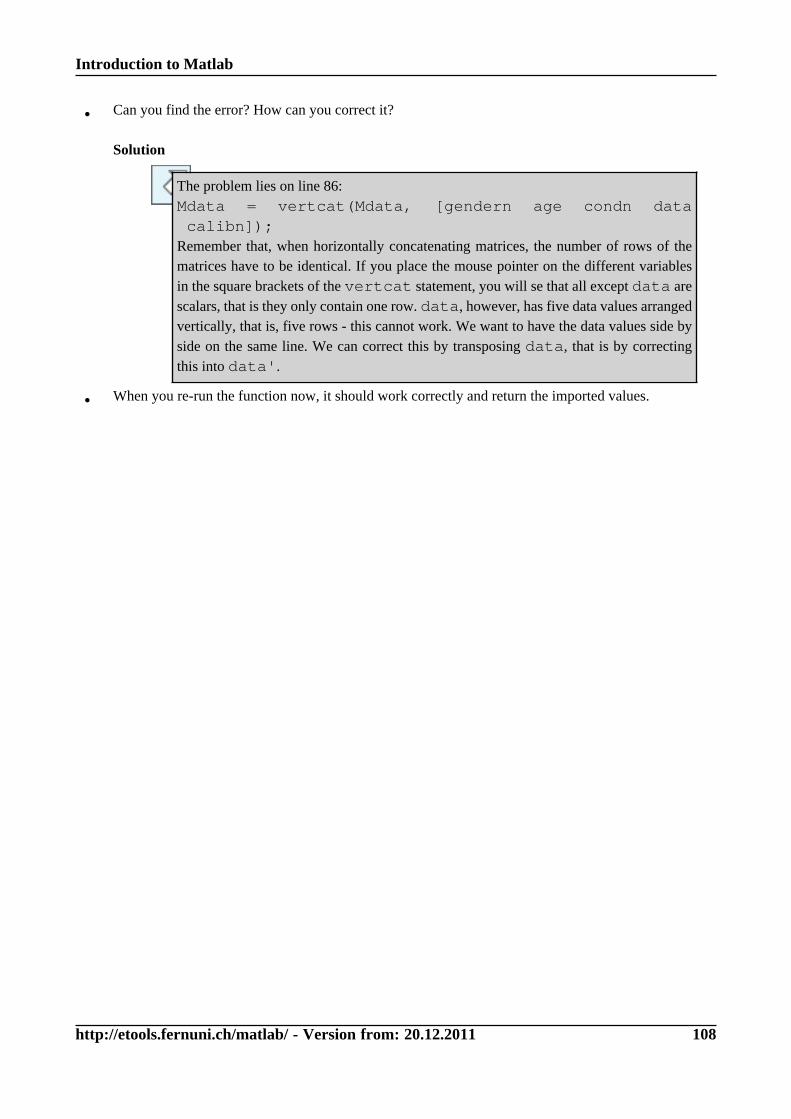
Introduction to Matlab
http://etools.fernuni.ch/matlab/ - Version from: 20.12.2011 108
• Can you find the error? How can you correct it?
Solution
The problem lies on line 86:Mdata = vertcat(Mdata, [gendern age condn data calibn]);Remember that, when horizontally concatenating matrices, the number of rows of thematrices have to be identical. If you place the mouse pointer on the different variablesin the square brackets of the vertcat statement, you will se that all except data arescalars, that is they only contain one row. data, however, has five data values arrangedvertically, that is, five rows - this cannot work. We want to have the data values side byside on the same line. We can correct this by transposing data, that is by correctingthis into data'.
• When you re-run the function now, it should work correctly and return the imported values.
Introduction to Matlab
http://etools.fernuni.ch/matlab/ - Version from: 20.12.2011 109
Summary
• fid = fopen(filename, mode): Opens a file
• data = fgetl(fid): reads one line
• data = fscanf(fid, format, n): Reads n data units in a certainformat, specified in format
• fclose(fid): closes a file
• feof(fid): checks whether the end of the file has been reached (eof = endof file)
Introduction to Matlab
http://etools.fernuni.ch/matlab/ - Version from: 20.12.2011 110
Data Representation 3: Cell ArraysIn this chapter you will get to know a different, comfortable way to represent data in Matlab: in so-called cellarrays.While matrices only accept numbers and - with certain restrictions - strings as their contents, a cell array allowsfor storing differing data types in every one of its data fields (= cells), especially matrices of different size.
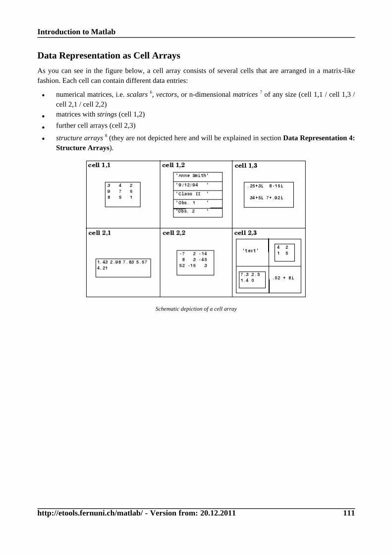
Introduction to Matlab
http://etools.fernuni.ch/matlab/ - Version from: 20.12.2011 111
Data Representation as Cell Arrays
As you can see in the figure below, a cell array consists of several cells that are arranged in a matrix-likefashion. Each cell can contain different data entries:
• numerical matrices, i.e. scalars 6, vectors, or n-dimensional matrices 7 of any size (cell 1,1 / cell 1,3 /cell 2,1 / cell 2,2)
• matrices with strings (cell 1,2)
• further cell arrays (cell 2,3)
• structure arrays 8 (they are not depicted here and will be explained in section Data Representation 4:Structure Arrays).
Schematic depiction of a cell array
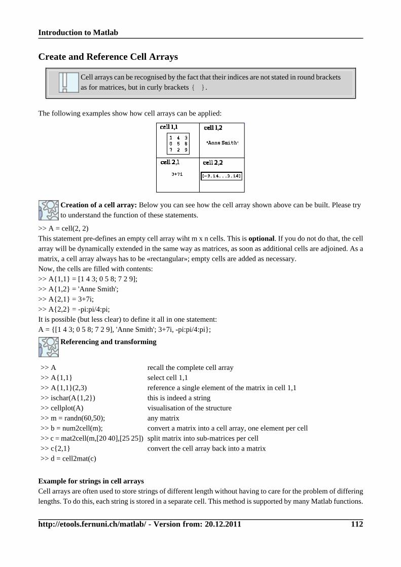
Introduction to Matlab
http://etools.fernuni.ch/matlab/ - Version from: 20.12.2011 112
Create and Reference Cell Arrays
Cell arrays can be recognised by the fact that their indices are not stated in round bracketsas for matrices, but in curly brackets { }.
The following examples show how cell arrays can be applied:
Creation of a cell array: Below you can see how the cell array shown above can be built. Please tryto understand the function of these statements.
>> A = cell(2, 2)This statement pre-defines an empty cell array wiht m x n cells. This is optional. If you do not do that, the cellarray will be dynamically extended in the same way as matrices, as soon as additional cells are adjoined. As amatrix, a cell array always has to be «rectangular»; empty cells are added as necessary.Now, the cells are filled with contents:>> A{1,1} = [1 4 3; 0 5 8; 7 2 9];>> A{1,2} = 'Anne Smith';>> A{2,1} = 3+7i;>> A{2,2} = -pi:pi/4:pi;It is possible (but less clear) to define it all in one statement:A = {[1 4 3; 0 5 8; 7 2 9], 'Anne Smith'; 3+7i, -pi:pi/4:pi};
Referencing and transforming
>> A>> A{1,1}>> A{1,1}(2,3)>> ischar(A{1,2})>> cellplot(A)>> m = randn(60,50);>> b = num2cell(m);>> c = mat2cell(m,[20 40],[25 25])>> c{2,1}>> d = cell2mat(c)
recall the complete cell arrayselect cell 1,1reference a single element of the matrix in cell 1,1this is indeed a stringvisualisation of the structureany matrixconvert a matrix into a cell array, one element per cellsplit matrix into sub-matrices per cellconvert the cell array back into a matrix
Example for strings in cell arraysCell arrays are often used to store strings of different length without having to care for the problem of differinglengths. To do this, each string is stored in a separate cell. This method is supported by many Matlab functions.
Introduction to Matlab
http://etools.fernuni.ch/matlab/ - Version from: 20.12.2011 113
An example:
>> texts = {'Hello world', 'The quick brown fox', num2str(pi), 'jumps over the lazy dog'}>> texts{4}>> length(texts{3})
Introduction to Matlab
http://etools.fernuni.ch/matlab/ - Version from: 20.12.2011 114
Second example on data import from external files
The previous example will now be changed in a way that (1) the name information is returned as a cell array,and (2) the data are not read in a loop by using fscanf, but with a single call of the function textscan,which also returns the data in a cell aray.
Please have a look at the function load_data2.m by following the steps described below.
• Open the function load_data2.m in the Editor
• On line 47 you see how textscan is applied.Cdata = textscan(fid, '%s %s %s %f %s %f %f %f %f %f %s');This statement reads data into a cell array until the end of the file has been reached. The format of thedata is defined in a format string (%s are strings, %f are floating point numbers). Cdata{x} will thencontain all data from column x. Alphanumerical data are stored as a cell array in a cell, the numericaldata as matrices.
• (regarding data processing, this function is intentionally left incomplete)
• on the lines 59-61, the data are re-configured according to the needs:Cfirstname = Cdata{1};Cfamilyname = Cdata{2};Mdata = [Cdata{4} Cdata{6:10}];
The function can be called by[Mdata, Cfirstname, Cfamilyname] = load_data2('exp1.dat').
Introduction to Matlab
http://etools.fernuni.ch/matlab/ - Version from: 20.12.2011 115
Summary
Points to remember
• A cell array consists of several cells that are arranged in a matrix-like way. Everycell can contain various kinds of data such as complete matrices, strings, furthrecell arrays or structure arrays.
• Cell arrays can be recognised by the fact that their indices are enclosed by curlybrackets { }, not round brackets as in matrices.
Commands
• cellplot: visualisation of the structure of a cell array
• num2cell: convert a matrix into a cell array, one element per cell
• mat2cell: divide matrix into sub-matrices per cell
• cell2mat: convert a cell array into a matrix
• textscan: read data from a file into a cell array
Introduction to Matlab
http://etools.fernuni.ch/matlab/ - Version from: 20.12.2011 116
Data Representation 4: Structure ArraysAnother useful way to represent data are the so-called structure arrays. Every element of a structure arraycontains the same structure of various «data containers» that are each referenced by a unique name. Compared
to cell arrays 9, it is more clearly visible what the contents of a referenced data field are.
9 A data structure that consists of several cells arranged in a matrix. Every cell can contain various kinds of data such as complete matrices,
strings, further cell arrays etc.
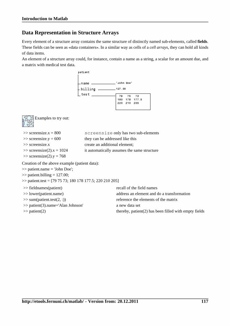
Introduction to Matlab
http://etools.fernuni.ch/matlab/ - Version from: 20.12.2011 117
Data Representation in Structure Arrays
Every element of a structure array contains the same structure of distinctly named sub-elements, called fields.These fields can be seen as «data containers». In a similar way as cells of a cell arrays, they can hold all kindsof data items.An element of a structure array could, for instance, contain a name as a string, a scalar for an amount due, anda matrix with medical test data.
Examples to try out:
>> screensize.x = 800>> screensize.y = 600>> screensize.x>> screensize(2).x = 1024>> screensize(2).y = 768
screensize only has two sub-elementsthey can be addressed like thiscreate an additional element;it automatically assumes the same structure
Creation of the above example (patient data):>> patient.name = 'John Doe';>> patient.billing = 127.00;>> patient.test = [79 75 73; 180 178 177.5; 220 210 205]
>> fieldnames(patient)>> lower(patient.name)>> sum(patient.test(2, :))>> patient(3).name='Alan Johnson'>> patient(2)
recall of the field namesaddress an element and do a transformationreference the elements of the matrixa new data setthereby, patient(2) has been filled with empty fields
Introduction to Matlab
http://etools.fernuni.ch/matlab/ - Version from: 20.12.2011 118
Application example
You could implement a function to import experiment data that stores all general data concerning theexperiment trial in a structure array. In this way, you can avoid having to return the data in many individualvariables.That is, instead of:function [Mdata, sex, age, eye, date, time] = loaddata(filename)you could implement it in this way:function [Mdata, expinfo] = loaddata(filename)expinfo would consist of the fields:expinfo.sexexpinfo.ageexpinfo.eyeexpinfo.dateexpinfo.time
Introduction to Matlab
http://etools.fernuni.ch/matlab/ - Version from: 20.12.2011 119
Summary
• Every element of a structure array contains the same structure of different «datacontainers» (fields) that are addressable with a name. Thus, contrary to cell arrays,it is clearly visible what a referenced data field contains.
• The fields are addressed by adding the field name to the variable name, separatedby a period: patient.name
Introduction to Matlab
http://etools.fernuni.ch/matlab/ - Version from: 20.12.2011 120
Your Data Processing ProjectNow, you know all basic building blocks to enable you to start writing a data processing program of your own.The final goal is to have a program that imports data from files, processes them (aggregation, conversion,graphical display etc.) and stores the results in a file.The project will be realised in several parts Px (P for project):
• Exercise P1: write the main program and the function to import the data
• Exercise P2: request user inputs
• Exercise P3: data processing and saving to an external file
• Exercise P4: computations
• Exercise P5: graphical visualisation of the data
Introduction to Matlab
http://etools.fernuni.ch/matlab/ - Version from: 20.12.2011 121
Data Base
Considering the data to be processed, there are several options for your project:
• You have data from your own research project that you want to process.
• If you do not have such a data set available, you can use the example project «EyeData Processing»provided by this course (it will be described later on).In this way, you can implement a kind of a template that might help you when you need to emplementa similar program later on.
• Alternatively, you can create a hypothetical practice data set (e.g. in Open Office Calc or MS Excel),similar to exp1.dat
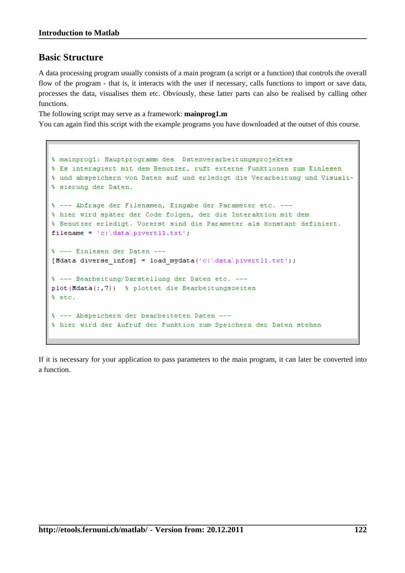
Introduction to Matlab
http://etools.fernuni.ch/matlab/ - Version from: 20.12.2011 122
Basic Structure
A data processing program usually consists of a main program (a script or a function) that controls the overallflow of the program - that is, it interacts with the user if necessary, calls functions to import or save data,processes the data, visualises them etc. Obviously, these latter parts can also be realised by calling otherfunctions.The following script may serve as a framework: mainprog1.mYou can again find this script with the example programs you have downloaded at the outset of this course.
If it is necessary for your application to pass parameters to the main program, it can later be converted intoa function.
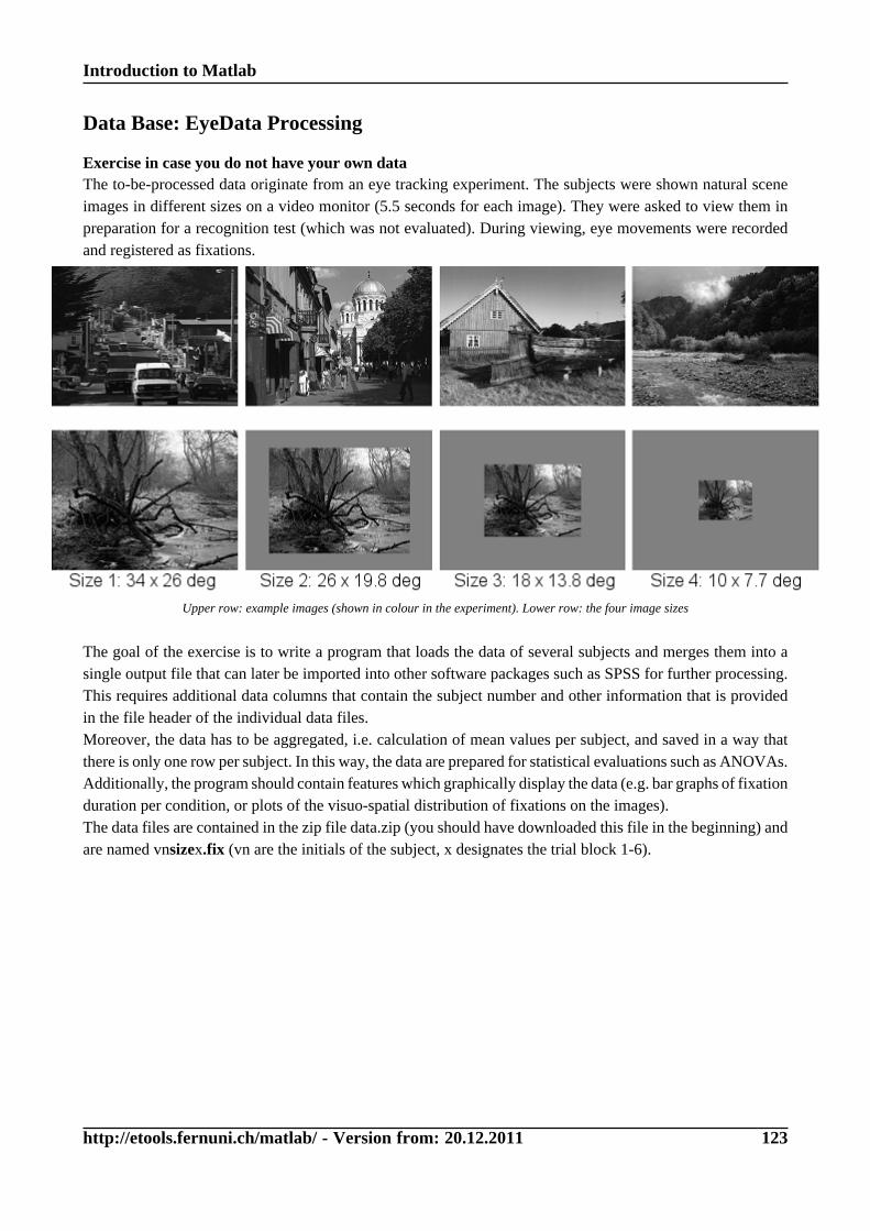
Introduction to Matlab
http://etools.fernuni.ch/matlab/ - Version from: 20.12.2011 123
Data Base: EyeData Processing
Exercise in case you do not have your own dataThe to-be-processed data originate from an eye tracking experiment. The subjects were shown natural sceneimages in different sizes on a video monitor (5.5 seconds for each image). They were asked to view them inpreparation for a recognition test (which was not evaluated). During viewing, eye movements were recordedand registered as fixations.
Upper row: example images (shown in colour in the experiment). Lower row: the four image sizes
The goal of the exercise is to write a program that loads the data of several subjects and merges them into asingle output file that can later be imported into other software packages such as SPSS for further processing.This requires additional data columns that contain the subject number and other information that is providedin the file header of the individual data files.Moreover, the data has to be aggregated, i.e. calculation of mean values per subject, and saved in a way thatthere is only one row per subject. In this way, the data are prepared for statistical evaluations such as ANOVAs.Additionally, the program should contain features which graphically display the data (e.g. bar graphs of fixationduration per condition, or plots of the visuo-spatial distribution of fixations on the images).The data files are contained in the zip file data.zip (you should have downloaded this file in the beginning) andare named vnsizex.fix (vn are the initials of the subject, x designates the trial block 1-6).
Introduction to Matlab
http://etools.fernuni.ch/matlab/ - Version from: 20.12.2011 124
Exercise P1: Data Import
Take the framework mainprog1.m for the main program outlined above and save it under a new namethat fits your project (eyedata.m for the example task «EyeData Processing». The sample solution forthis task can be found under the file name eyedata_sol1.m).
Write a new function to import your data from the external files. To do this, you can start from scratch, oryou modify and extend load_data1.m used in an earlier example (it is recommended to save it with a newname as well).If you have your own data set, please first consider what you want to do with your data. This will influence theway your function will have to return the imported data to the calling script. Relevant questions are:
• Which of the available data are needed for further processing?
• Are there certain data items that need to be recoded (typical case: conversion of experimental conditionscoded in clear text into numerical codes)?
• Which data structures are best suited for further processing - single values, matrices, cell arrays, orstructure arrays?
Guidelines for the «EyeData Processing» projectTry to implement a function readfixdata.m that reads a single data file and returns the data in suitable form,e.g. as
• a structure array with the fields study name, subject number, recording date, left/right eye, number ofimages, and screen resolution
• a cell array with the image names;
• and a matrix containing the eye movement data.
These suggestions refer to the sample solution, but - of course - there is not a single correct solution; it is justas well possible to pack everything into a cell array, for instance.The data to process have the following stucture (afsize1.fix, tab-separated file):
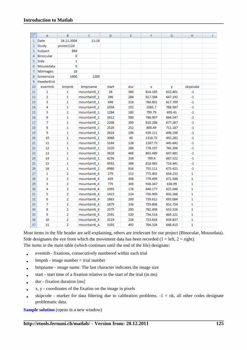
Introduction to Matlab
http://etools.fernuni.ch/matlab/ - Version from: 20.12.2011 125
Most items in the file header are self-explaining, others are irrelevant for our project (Binocular, Mousedata).Side designates the eye from which the movement data has been recorded (1 = left, 2 = right).The items in the main table (which continues until the end of the file) designate:
• eventnb - fixations, consecutively numbered within each trial
• bmpnb - image number = trial number
• bmpname - image name. The last character indicates the image size
• start - start time of a fixation relative to the start of the trial (in ms)
• dur - fixation duration [ms]
• x, y - coordinates of the fixatins on the image in pixels
• skipcode - marker for data filtering due to calibration problems. -1 = ok, all other codes designateproblematic data.
Sample solution (opens in a new window)

Introduction to Matlab
http://etools.fernuni.ch/matlab/ - Version from: 20.12.2011 126
The solution can also be found in the M-file readfixdata_sol.m.
Introduction to Matlab
http://etools.fernuni.ch/matlab/ - Version from: 20.12.2011 127
User InteractionMost larger applications require a certain amount of interaction with the user. Typical examples are:
• Selections of data files to be processed
• Specification of parameters such as limits, filter settings, selection of graphics options etc.
• Graphical inputs, e.g. definition of «regions of interests» (ROIs) or calibration points by means of mouseclicks
• Selection of the location and file format for saving data or graphics
Below, the most important interactive elements are listed. However, the implementation of integrated graphicaluser interfaces (GUIs) will not be discussed.
Cf. the information given in the Help System under MATLAB > Function Reference > CreatingGraphical User Interfaces.
Introduction to Matlab
http://etools.fernuni.ch/matlab/ - Version from: 20.12.2011 128
Selection of Files and Directories
Standard dialog boxes to select files or directory locations for loading and saving data as you know them fromother applications are also available in Matlab.
All of them have a large number of configuration options, which cannot be discussed in detail here,thus only some typical application examples are shown. For further options, please consult the HelpSystem.
Select a file: uigetfile[FileName, PathName] = uigetfile('*.m', 'Select the M-file');Opens the file selection dialog box. The function returns the file name and the path. If «Cancel» has beenclicked, FileName = 0 results.The first argument '*.m' is a filter, i.e. only files with this extension are shown. If all files should be visible,'*.*' can be entered. The second argument contains the text that will be shown in the window title.The selection process begins at the current path as it is set in Matlab as the «Current Directory».If you want the selection to start at a different place in the file system, you can specify it like this:[FileName,PathName] = ...uigetfile('d:\matlab\data\*.txt', 'Select data set');If several file types should be available, you can specify this by means of a cell array. The desired file extensionsare listed in the first column of the cell array:[filename, pathname] = ...uigetfile({'*.m'; '*.mdl'; '*.mat'; '*.*'}, 'File Selector');
Example for a file selection dialog with output of the result. Copy the code lines below into theCommand Window (>> can also be copied - Matlab will ignore them).
>> [filename, pathname] = uigetfile('*.txt', 'Pick a text file');>> if isequal(filename, 0)>> disp('User selected ''Cancel''')>> else>> disp(['User selected ', fullfile(pathname, filename)])>> end
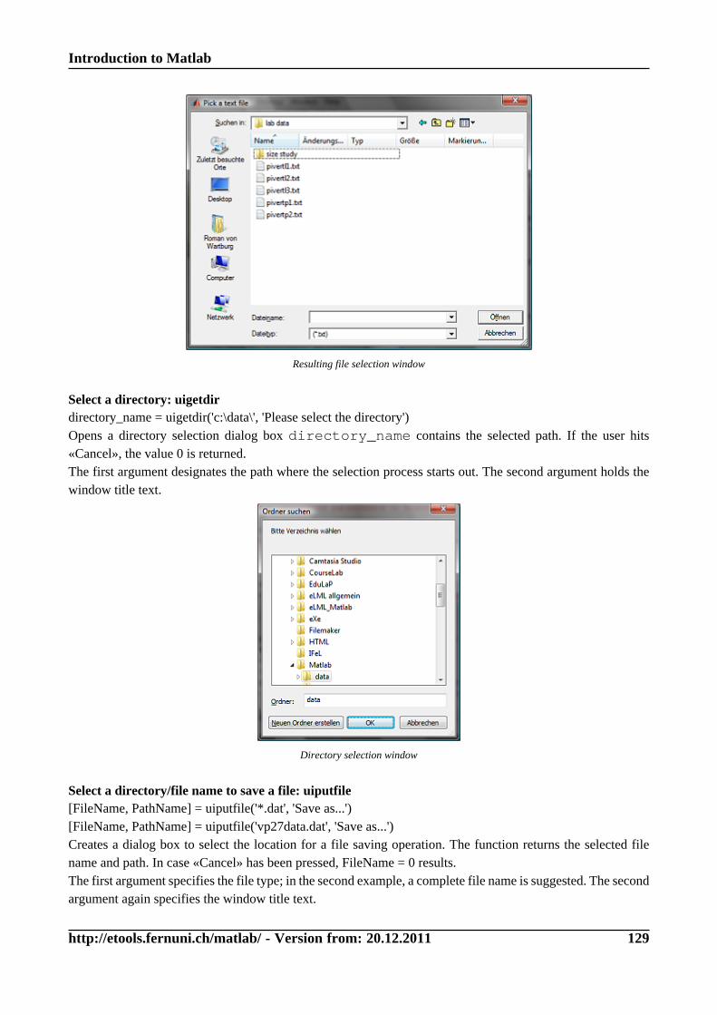
Introduction to Matlab
http://etools.fernuni.ch/matlab/ - Version from: 20.12.2011 129
Resulting file selection window
Select a directory: uigetdirdirectory_name = uigetdir('c:\data\', 'Please select the directory')Opens a directory selection dialog box directory_name contains the selected path. If the user hits«Cancel», the value 0 is returned.The first argument designates the path where the selection process starts out. The second argument holds thewindow title text.
Directory selection window
Select a directory/file name to save a file: uiputfile[FileName, PathName] = uiputfile('*.dat', 'Save as...')[FileName, PathName] = uiputfile('vp27data.dat', 'Save as...')Creates a dialog box to select the location for a file saving operation. The function returns the selected filename and path. In case «Cancel» has been pressed, FileName = 0 results.The first argument specifies the file type; in the second example, a complete file name is suggested. The secondargument again specifies the window title text.
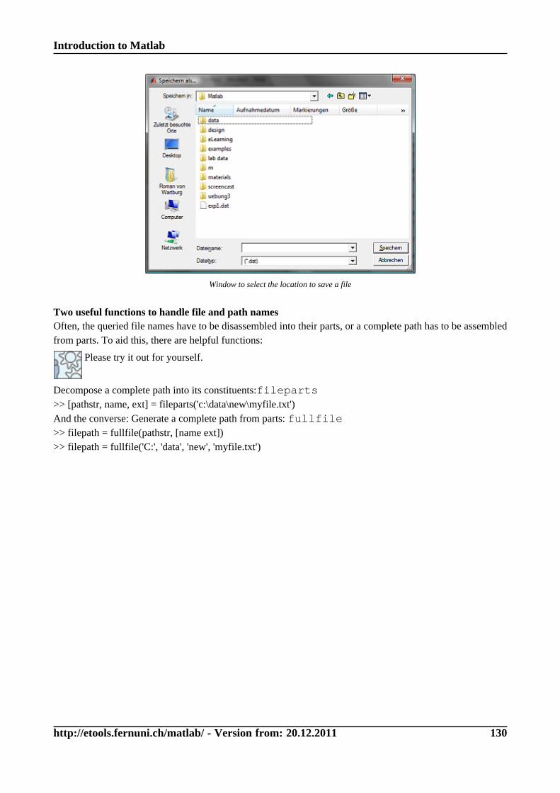
Introduction to Matlab
http://etools.fernuni.ch/matlab/ - Version from: 20.12.2011 130
Window to select the location to save a file
Two useful functions to handle file and path namesOften, the queried file names have to be disassembled into their parts, or a complete path has to be assembledfrom parts. To aid this, there are helpful functions:
Please try it out for yourself.
Decompose a complete path into its constituents:fileparts>> [pathstr, name, ext] = fileparts('c:\data\new\myfile.txt')And the converse: Generate a complete path from parts: fullfile>> filepath = fullfile(pathstr, [name ext])>> filepath = fullfile('C:', 'data', 'new', 'myfile.txt')
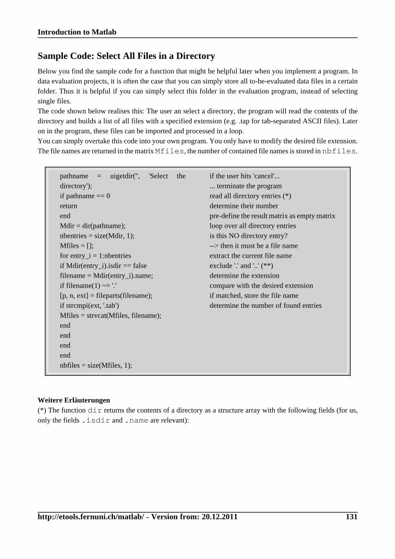
Introduction to Matlab
http://etools.fernuni.ch/matlab/ - Version from: 20.12.2011 131
Sample Code: Select All Files in a Directory
Below you find the sample code for a function that might be helpful later when you implement a program. Indata evaluation projects, it is often the case that you can simply store all to-be-evaluated data files in a certainfolder. Thus it is helpful if you can simply select this folder in the evaluation program, instead of selectingsingle files.The code shown below realises this: The user an select a directory, the program will read the contents of thedirectory and builds a list of all files with a specified extension (e.g. .tap for tab-separated ASCII files). Lateron in the program, these files can be imported and processed in a loop.You can simply overtake this code into your own program. You only have to modify the desired file extension.The file names are returned in the matrix Mfiles, the number of contained file names is stored in nbfiles.
pathname = uigetdir('', 'Select thedirectory');if pathname == 0returnendMdir = dir(pathname);nbentries = size(Mdir, 1);Mfiles = [];for entry_i = 1:nbentriesif Mdir(entry_i).isdir == falsefilename = Mdir(entry_i).name;if filename(1) ~= '.'[p, n, ext] = fileparts(filename);if strcmpi(ext, '.tab')Mfiles = strvcat(Mfiles, filename);endendendendnbfiles = size(Mfiles, 1);
if the user hits 'cancel'...... terminate the programread all directory entries (*)determine their numberpre-define the result matrix as empty matrixloop over all directory entriesis this NO directory entry?--> then it must be a file nameextract the current file nameexclude '.' and '..' (**)determine the extensioncompare with the desired extensionif matched, store the file namedetermine the number of found entries
Weitere Erläuterungen(*) The function dir returns the contents of a directory as a structure array with the following fields (for us,only the fields .isdir and .name are relevant):
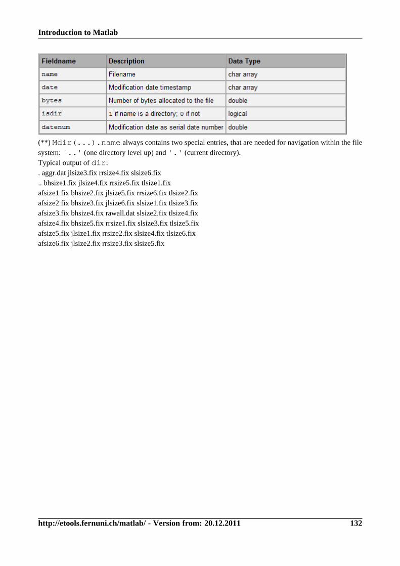
Introduction to Matlab
http://etools.fernuni.ch/matlab/ - Version from: 20.12.2011 132
(**) Mdir(...).name always contains two special entries, that are needed for navigation within the filesystem: '..' (one directory level up) and '.' (current directory).Typical output of dir:. aggr.dat jlsize3.fix rrsize4.fix slsize6.fix.. bhsize1.fix jlsize4.fix rrsize5.fix tlsize1.fixafsize1.fix bhsize2.fix jlsize5.fix rrsize6.fix tlsize2.fixafsize2.fix bhsize3.fix jlsize6.fix slsize1.fix tlsize3.fixafsize3.fix bhsize4.fix rawall.dat slsize2.fix tlsize4.fixafsize4.fix bhsize5.fix rrsize1.fix slsize3.fix tlsize5.fixafsize5.fix jlsize1.fix rrsize2.fix slsize4.fix tlsize6.fixafsize6.fix jlsize2.fix rrsize3.fix slsize5.fix
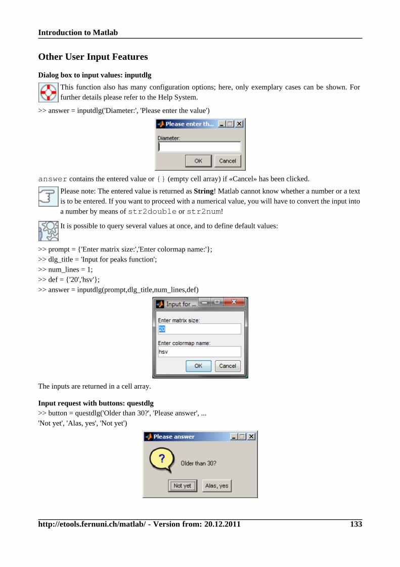
Introduction to Matlab
http://etools.fernuni.ch/matlab/ - Version from: 20.12.2011 133
Other User Input Features
Dialog box to input values: inputdlg
This function also has many configuration options; here, only exemplary cases can be shown. Forfurther details please refer to the Help System.
>> answer = inputdlg('Diameter:', 'Please enter the value')
answer contains the entered value or {} (empty cell array) if «Cancel» has been clicked.
Please note: The entered value is returned as String! Matlab cannot know whether a number or a textis to be entered. If you want to proceed with a numerical value, you will have to convert the input intoa number by means of str2double or str2num!
It is possible to query several values at once, and to define default values:
>> prompt = {'Enter matrix size:','Enter colormap name:'};>> dlg_title = 'Input for peaks function';>> num_lines = 1;>> def = {'20','hsv'};>> answer = inputdlg(prompt,dlg_title,num_lines,def)
The inputs are returned in a cell array.
Input request with buttons: questdlg>> button = questdlg('Older than 30?', 'Please answer', ...'Not yet', 'Alas, yes', 'Not yet')
Introduction to Matlab
http://etools.fernuni.ch/matlab/ - Version from: 20.12.2011 134
Explanations: The last argument designates which button will be set as the «default», that is it will already bepre-selected (and can be confirmed with the enter key). This argument cannot be omitted.button will return the clear text of the selected button. It is just as well possible to create more than twobuttons.
You can find many more options in the Help System under the keyword «Predefined Dialog Boxes».
Graphical input of coordinates: ginputWith this function, coordinates can be entered in an existing graph.
Please have a look at this:
>> plot(peaks) % create any graphic>> hold on>> [x, y] = ginput(3)>> plot(x, y, '.-r')>In this example, three values are queried. By means of the return key, the input process can be terminatedearlier. The coordinates are returned in the column vectors x and y.
Introduction to Matlab
http://etools.fernuni.ch/matlab/ - Version from: 20.12.2011 135
Exercise P2: User Inputs
Integrate the necessary user inputs into your project's main program. Dependent on your actual goals,various inputs can be necessary:
• Selection of the file(s) to be processed, or the directory where the data are stored.
• Query any parameters that are necessary for data processing (i.e. filter settings)
• Selection of the file name and/or the storing location for saving the processed data.
• Ask the user whether certain evaluations or graphical outputs are desired.
If no file has been selected in the file selection process («cancel» has been pressed), the program should exitand return an appropriate message. Other erroneous inputs should either be made impossible, or lead to anerror message.
For the EyeData project
• First, the user should be able to select a fixation file (that is, a file with the extension .fix).
• As a parameter, the user has to be asked whether s/he wants the data to be filtered based on the datain the column skipcode.
• Moreover, the user has to enter where and under which name the data (the merged raw data file and theaggregated data) are to be saved.
You can find the sample solution in the M-file eyedata_sol2.m
Introduction to Matlab
http://etools.fernuni.ch/matlab/ - Version from: 20.12.2011 136
Summary
Summary of the most important commands:
• uigetfile: dialog box to select a file
• uigetdir: dialog box to select s folder (directory)
• uiputfile: dialog box to select the location to save a file
• fileparts: decomposes a complete path into its parts
• fullfile: creates a complete path from parts
• inputdlg: dialog box to query values
• questdlg: dialog box with buttons
• ginput: graphical input of coordinates
• dir: read directory entries from the file system

Introduction to Matlab
http://etools.fernuni.ch/matlab/ - Version from: 20.12.2011 137
Writing Data to External FilesBasically, the procedure is very similar to reading from external files: First, the file is opened with fopen,then the data is written, and finally, the file has to be closed again with fclose.
Introduction to Matlab
http://etools.fernuni.ch/matlab/ - Version from: 20.12.2011 138
Basic Functions to Write to External Files
Some of the commands described below have further parameters - please refer to the Help System ifnecessary.
fid = fopen(filename, mode)Opens a file. Now, as mode, 'w' (write - open a file for writing or creating) or 'a' (append data to theexisting file) has to be selected.fprintf(fid, format, M, ...)Writes the data contained in the matrix M (and any further matrices) to the file. The format of the written datais controlled by the format string.
There are extensive options how the data can be formatted by means of the format string. Some basicformats are shown in the example below. For the detailed format specifications and all further optionsplease consult the Help System.
fclose(fid)Closes the file. Only after closing, other applications can freely access the file.
Example: Writing to a fileAlso see the M-file m-File writedatafile.m
% open the file in write modefid = fopen('C:\m\testdata.txt', 'w');% Write text:% %s designates a string, \n generates a line breakfprintf(fid, '%s\n', 'Any text');% Schreiben von numerischen Daten:% %g stands for fixed point notation, several values are written% and separated by a tabulator (\t).fprintf(fid, '%g\t', pi, [7.5:3:13.5]);fprintf(fid, '\n'); % write the line break% output with maximally 6 integer digits and 2 decimal digitsfprintf(fid, '%6.2f\t', [737.5:3234.273:20000]);% close the filefclose(fid);
This example generates the data file C:\m\testdata.txt (as viewed in MS Excel):
Introduction to Matlab
http://etools.fernuni.ch/matlab/ - Version from: 20.12.2011 139
You can find further file functions in the Help System, e.g. under: MATLAB > Function Reference> File I/O > Text files
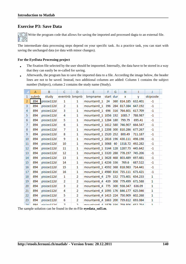
Introduction to Matlab
http://etools.fernuni.ch/matlab/ - Version from: 20.12.2011 140
Exercise P3: Save Data
Write the program code that allows for saving the imported and processed dagta to an external file.
The intermediate data processing steps depend on your specific task. As a practice task, you can start withsaving the unchanged data (or data with minor changes).
For the EyeData Processing project
• The fixation file selected by the user should be impoorted. Internally, the data have to be stored in a waythat they can easily be re-called for saving.
• Afterwards, the program has to save the imported data to a file. According the image below, the headerlines are not to be saved. Instead, two additional columns are added: Column 1 contains the subjectnumber (Subject), column 2 contains the study name (Study).
The sample solution can be found in the m-File eyedata_sol3.m.
Introduction to Matlab
http://etools.fernuni.ch/matlab/ - Version from: 20.12.2011 141
Summary
Summary of the most important points and commands:
Points to remember
• The procedure when writing data to a file is the almost the same as when reading:First, the file is opened by fopen, then data are written with fprintf, andfinally, the file has to be closed by fclose.
Commands
• fid = fopen(filename, mode): open a file
• fprintf(fid, format, M): write the data in matrix M to the file,formatted according to the format string
• fclose(fid): close a file
Introduction to Matlab
http://etools.fernuni.ch/matlab/ - Version from: 20.12.2011 142
GlossaryASCII:
American Standard Code for Information Interchange; the most common norm to represent alphanumericalcharacters.
cell array:A data structure that consists of several cells arranged in a matrix. Every cell can contain various kinds ofdata such as complete matrices, strings, further cell arrays etc.
copy-and-paste:On PC/Windows: CTRL-C and CTRL-V. On Mac OS: cmd-C and cmd-V
Debugger:Editor function to assist in finding and correcting errors in a program.
matrix:The most important way to represent data in Matlab. In the field of mathematics, a matrix is a table ofnumbers or other values. Matrices differ from ordinary tables in that they can be used for calculations.Usually, the expression «matrix» refers to two- or higher-dimensional matrices (cf. scalar, vector).
scalar:«null-dimensional» matrix, i.e. only one element
string:Character string. A vector or a matrix whose elements are interpreted as ASCII coded characters.
structure array:Every element of a structure array contains the same structure of various sub-elements that can be accessedwith a unique name, called fields. These fields can be seen as «data containers» that can hold all kinds ofcontents.
vector:one-dimensional matrix, that is only one row or one column
Introduction to Matlab
http://etools.fernuni.ch/matlab/ - Version from: 20.12.2011 143
Lesson 4: Data Processing and GraphicalPresentationThis lesson will show you how to further process data. On the one hand, it is about transformation, conversion,or aggregation of data, and computation of statistical characteristics. On the other hand, basic methods of datavisualisation are introduced.
Learning Objectives
• You know how to selectively access data.
• You know the most important statistical functions.
• You know how to generate graphical figures and how to adapt them to your needs.
• You know the most important graphical functions and can apply them to your data.
Introduction to Matlab
http://etools.fernuni.ch/matlab/ - Version from: 20.12.2011 144
Data Selection: Logical Indexing and the «find» FunctionThis section introduces important possibilities to selectively extract certain data from larger data fields. To thisend, the following methods are available:
• logical indexing
• the find function
• a dedicated function subM
Afterwards, your data processing project will be complemented by data evaluation functions.
Introduction to Matlab
http://etools.fernuni.ch/matlab/ - Version from: 20.12.2011 145
Logical Indexing
This data access method allows for addressing specific elements of a matrix based on logical comparisons. Putmore simply, you can address all elements fulfilling a certain condition at once. For example:>> a = magic(7);>> a(a < 10) = 0What has happened? All elements of a that are smaller than 10 are set to 0.And how does it work? The comparison a < 10 yields a matrix of the same size that contains the truthvalues of that comparison for every element. As you see now, comparison operators can also be applied towhole vectors or matrices! (cf. section Comparison Operators in Lesson 2). This resulting truth value matrixcan be used as logical index to access the values in the data matrix.
Now try it out yourself:
>> a = magic(7);>> a < 10>> b = a(a > 20)
result of the comparisonextracts all elements that fulfill the condition
It often happens that you need to extract data from a larger matrix according to certain criteria, e.g. the valuesfrom column 7 of all rows of a matrix Mdata whose column 3 contains a value larger than 0.5. An obvioussolution for that problem is to write a loop and check every row by means of an if statement and, if thecondition is met, extract the value from the desired column:
Mdata = rand(50, 7);Mselect = [];[nbrows, nbcols] = size(Mdata);for row_i = 1:nbrowsif Mdata(row_i, 3) > .5Mselect = vertcat(Mselect, Mdata(row_i, 7));endend
This can be realised with logical indexing in a much shorter and thus more elegant (and faster) manner:
>> Mdata = rand(50, 7);>> Mselect = Mdata(Mdata(:,3)>.5, 7)To clearly see how this works, we take a closer look at the «inner» expression:>> Mdata(:,3)>.5As you see, it yields a vector with the truth values of the comparison of all values in column 3 with the value0.5. This vector can now be used as a logical index into a matrix. That is, all columns whose correspondingentry contains true (a numerical value of 1) are selected.
Introduction to Matlab
http://etools.fernuni.ch/matlab/ - Version from: 20.12.2011 146
The find Function
The find function provides similar possibilities as the logical indexing discussed above. As a result, however,it does not return a matrix with logical indices, but a vector with the «linear indices» (cf. Lesson 1, sectionMatrices, paragraph «Linear Indexing» all the way down on the page).
Again, it is best to try it out:
>> a = magic(10);>> selected = find(a > 50)>> length(selected)
find all elements of a that are > 50number of matching elements
This now results in a vector with the linear indices of the matching elements. It can be used for furtheroperations:
>> b = a(selected)>> a(selected) = inf
extract the corresponding elementsset those elements in a to inf
In most cases, find can be replaced by logical indexing. Usually, this makes sense as this is processedfaster.
Introduction to Matlab
http://etools.fernuni.ch/matlab/ - Version from: 20.12.2011 147
A Helpful Function: subM
You can find this useful function (which is not included in the standard function set of Matlab) with the exampleprograms (zip file). It is defined like this:function Mselected = subM(Min, col, min, max)subM is a function that extracts all rows from a matrix Min whose value in column col lies within a definedrange from min and max (inclusive).>> M1 = magic(10);>> column = 3; minvalue = 10; maxvalue = 30;>> Mnew = subM(M1, column, minvalue, maxvalue)Of course, it is possible to program this directly using logical indexing. However, this is less comfortable andresults in a code that is more difficult to read :>> Mnew = M1(M1(:, column) >= minvalue & M1(:, column) <= maxvalue, :)Explanation: The results of the two comparisons are logically combined with & (AND operation). Let's lookat this in detail again:>> M1(:, column) >= minvalue>> M1(:, column) <= maxvalue>> M1(:, column) >= minvalue & M1(:, column) <= maxvalueIf you have a look at the function subM in the Editor (by typing edit subM), you see that - except fora plausibility check - it does not do anything else. Nevertheless, it can be helpful to write such often usedoperations as functions. This will later save time, and you get code that is easier to understand.
Introduction to Matlab
http://etools.fernuni.ch/matlab/ - Version from: 20.12.2011 148
Summary
Points to remember
• Logical indexing: A data access method that is used to address at once all elementsof a matrix that satisfy a certain condition.e.g. reading all elements from a that are smaller than 10: b = a(a < 10)
Commands
• find: Find elements in a matrix. As a result, the linear indices to the matchingelements are returned.
• subM: A help function (not included in Matlab's library). Extracts all rows froma matrix in which the value in a certain column lies in a defined range.
Introduction to Matlab
http://etools.fernuni.ch/matlab/ - Version from: 20.12.2011 149
Basic Statistical FunctionsIn this chapter, basic statistical functions included in the base version of Matlab are introduced. That is,
• functions to calculate statistical characteristics (descriptive statistics)
• calculation of correlation and covariance values
• functions to generate random data sets with defined distributions
Introduction to Matlab
http://etools.fernuni.ch/matlab/ - Version from: 20.12.2011 150
Descriptive Statistics
Even the basic version of Matlab offers a set of mainly descriptive statistics functions. Further functions areincluded in the Statistics Toolbox for Matlab, which has to be licensed separately. Its functions are thus notdiscussed here.
In case you have access to the Statistics Toolbox, you can find all necessary information in the HelpSystem under Statistics Toolbox (main category in the Contents part)
Minimum and maximumThe functions are called min and max. They can both be used in the same way:
Try it out:
>> a = magic(5);>> min(a)>> max(max(a))>> b=fix(rand(5)*25)>> max(a, b)>> min(a, [], 2)
calculates the minima in columns.calculates the minimum or maximum of a complete tabledefine a second matrixCompares a and b element by elementand writes the maximum of each comparison in a matrix of the same size.Of course, a and b have to be of the same size.In this way, you can specify the dimension of the calculation.1 are columns (default), 2 are rows, 3 are «planes», etc.
Mean, median, and modal valuesThere are three functions that have the same structure: mean, median, and mode.
Again, you best see for yourself:
>> m=fix(randn(200,6)*18+48);>> mean(m)>> modeval=mode(m)>> [vals,freq]=mode(m)>> median(m,2)
matrix with normally distributed valuesmean in columnsmodal value, i.e. the most frequent valuein this way you can also get the numbers of valuesYou can specify the dimension, too.
If you want to determine the value for a complete array, you first have to convert it into a column vector. A«logical solution» for this would be:m1 = reshape(m, numel(m), 1);But there's a «short cut»:
>> m1 = m(:)>> mode(m1)>> mean(m(:))
m(:) means: just take ALL values of mor even more directly
Variance and standard deviationThe two functions var and std are usually used in their most simple form (for details see the Help System).It will also calculate the values in columns.
Please study the examples below:
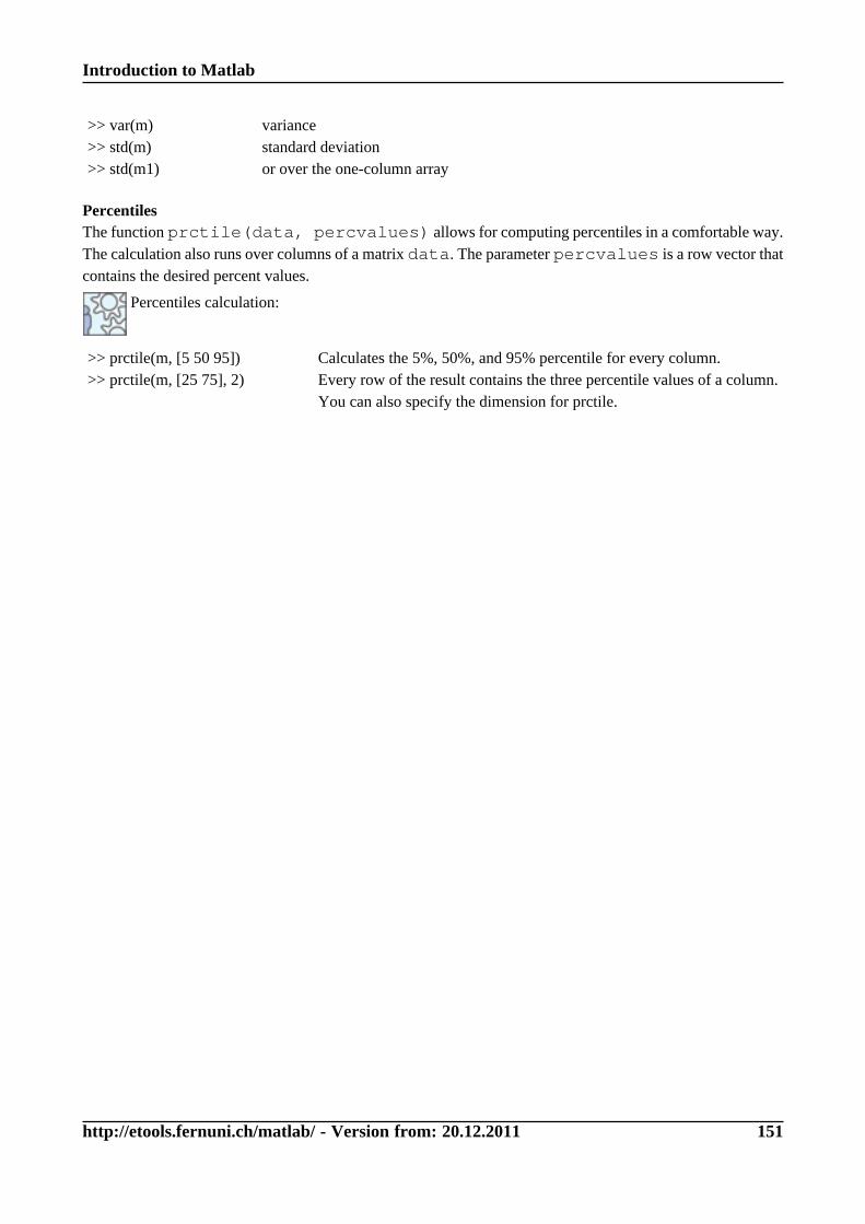
Introduction to Matlab
http://etools.fernuni.ch/matlab/ - Version from: 20.12.2011 151
>> var(m)>> std(m)>> std(m1)
variancestandard deviationor over the one-column array
PercentilesThe function prctile(data, percvalues) allows for computing percentiles in a comfortable way.The calculation also runs over columns of a matrix data. The parameter percvalues is a row vector thatcontains the desired percent values.
Percentiles calculation:
>> prctile(m, [5 50 95])>> prctile(m, [25 75], 2)
Calculates the 5%, 50%, and 95% percentile for every column.Every row of the result contains the three percentile values of a column.You can also specify the dimension for prctile.
Introduction to Matlab
http://etools.fernuni.ch/matlab/ - Version from: 20.12.2011 152
Correlation and Covariance
The only inference statistics function of Matlab in its basic version is the calculation of correlations withcorrcoef. The most important formats are:R = corrcoef(X)Yields a matrix R with the correlation coefficients. The function runs over a two-dimensional matrix, whichis interpreted as follows: The columns represent the dependent variables, and the rows represent theindividual observations (that is, the measured values).R = corrcoef(x, y)x and y are column vectors corresponding to two dependent variables. More precisely, if x and y are notcolumn vectors, they will automatically be converted into column vectors. Obviously, the number of elementsin both arrays need to be the same.[R, P, RLO, RUP] = corrcoef(X, 'alpha', .01)In this way, you obtain further values. P contains the significance values based on the specified alpha value.The parameter alpha can be omitted - the default value will then be .05 for 95% confidence interval.RLO and RUP contain the lower and upper limits for a 95% confidence interval for every correlationcoefficient.
As usual, you can find the details on further parameters in the Help System.
To illustrate this, an example from the Help System is shown. A data matrix which includes acorrelation between column 4 and the other columns is used.
>> x = randn(30, 4);>> x(:, 4) = sum(x, 2);>> [r, p] = corrcoef(x)>> [i, j] = find(p < 0.05);>> [i, j]
uncorrelated random datanow we generate a correlationcalculate correlation coefficients and p valuesfind the significant correlations (columns, rows)display their columns and rows
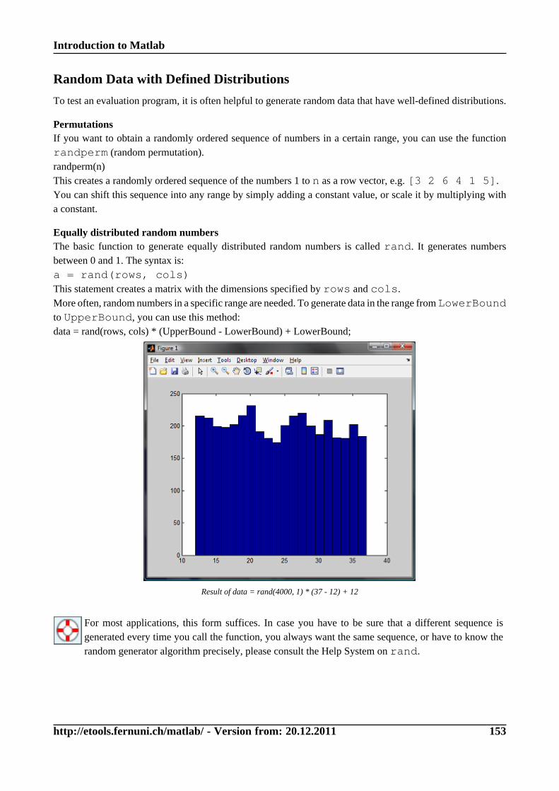
Introduction to Matlab
http://etools.fernuni.ch/matlab/ - Version from: 20.12.2011 153
Random Data with Defined Distributions
To test an evaluation program, it is often helpful to generate random data that have well-defined distributions.
PermutationsIf you want to obtain a randomly ordered sequence of numbers in a certain range, you can use the functionrandperm (random permutation).randperm(n)This creates a randomly ordered sequence of the numbers 1 to n as a row vector, e.g. [3 2 6 4 1 5].You can shift this sequence into any range by simply adding a constant value, or scale it by multiplying witha constant.
Equally distributed random numbersThe basic function to generate equally distributed random numbers is called rand. It generates numbersbetween 0 and 1. The syntax is:a = rand(rows, cols)This statement creates a matrix with the dimensions specified by rows and cols.More often, random numbers in a specific range are needed. To generate data in the range from LowerBoundto UpperBound, you can use this method:data = rand(rows, cols) * (UpperBound - LowerBound) + LowerBound;
Result of data = rand(4000, 1) * (37 - 12) + 12
For most applications, this form suffices. In case you have to be sure that a different sequence isgenerated every time you call the function, you always want the same sequence, or have to know therandom generator algorithm precisely, please consult the Help System on rand.
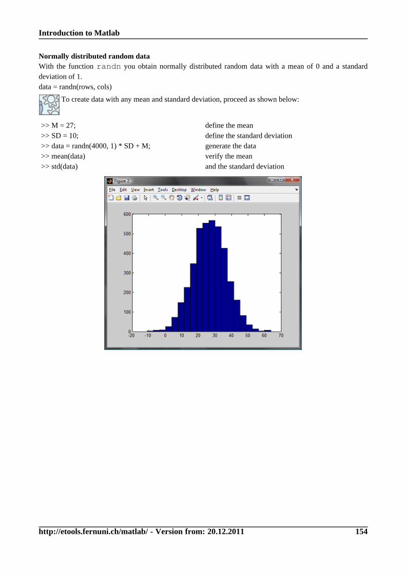
Introduction to Matlab
http://etools.fernuni.ch/matlab/ - Version from: 20.12.2011 154
Normally distributed random dataWith the function randn you obtain normally distributed random data with a mean of 0 and a standarddeviation of 1.data = randn(rows, cols)
To create data with any mean and standard deviation, proceed as shown below:
>> M = 27;>> SD = 10;>> data = randn(4000, 1) * SD + M;>> mean(data)>> std(data)
define the meandefine the standard deviationgenerate the dataverify the meanand the standard deviation
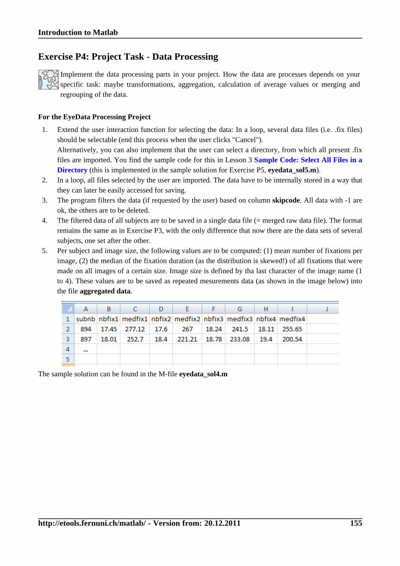
Introduction to Matlab
http://etools.fernuni.ch/matlab/ - Version from: 20.12.2011 155
Exercise P4: Project Task - Data Processing
Implement the data processing parts in your project. How the data are processes depends on yourspecific task: maybe transformations, aggregation, calculation of average values or merging andregrouping of the data.
For the EyeData Processing Project
1. Extend the user interaction function for selecting the data: In a loop, several data files (i.e. .fix files)should be selectable (end this process when the user clicks "Cancel").Alternatively, you can also implement that the user can select a directory, from which all present .fixfiles are imported. You find the sample code for this in Lesson 3 Sample Code: Select All Files in aDirectory (this is implemented in the sample solution for Exercise P5, eyedata_sol5.m).
2. In a loop, all files selected by the user are imported. The data have to be internally stored in a way thatthey can later be easily accessed for saving.
3. The program filters the data (if requested by the user) based on column skipcode. All data with -1 areok, the others are to be deleted.
4. The filtered data of all subjects are to be saved in a single data file (= merged raw data file). The formatremains the same as in Exercise P3, with the only difference that now there are the data sets of severalsubjects, one set after the other.
5. Per subject and image size, the following values are to be computed: (1) mean number of fixations perimage, (2) the median of the fixation duration (as the distribution is skewed!) of all fixations that weremade on all images of a certain size. Image size is defined by tha last character of the image name (1to 4). These values are to be saved as repeated mesurements data (as shown in the image below) intothe file aggregated data.
The sample solution can be found in the M-file eyedata_sol4.m
Introduction to Matlab
http://etools.fernuni.ch/matlab/ - Version from: 20.12.2011 156
Summary
• min, max: minimum and maximum
• mean, mode, median: mean, modal, and median value
• var, std: variance and standard deviation
• prctile: calculation of percentiles
• corrcoef: correlation coefficients
• randperm: randomly ordered sequence of the numbers 1 to n
• rand: equally distributed random numbers between 0 and 1
• randn: normally distributed random numbers with mean 0 and standarddeviation 1
• data = rand(rows, cols) * (UpperBound - LowerBound) + LowerBound;generating random numbers in a defined range
Introduction to Matlab
http://etools.fernuni.ch/matlab/ - Version from: 20.12.2011 157
Graphics Basics: Figures and Axes
General information on graphics in MatlabMatlab provides extensive possibilities to graphically display data. It would go beyond the scope of this courseto give a comprehensive overview of all features. Instead of that, the basic mechanisms are introduced, togetherwith a demonstration of those graphics that are most often used in our field.
• handling figure windows
• interactive modification of graphics
• axes
• universal plots
• bar graphs
• a short demo of other graphs
• annotation and extension of graphics
Introduction to Matlab
http://etools.fernuni.ch/matlab/ - Version from: 20.12.2011 158
Creation and Manipulation of Figures
Every graphical output takes place in a special window, a so-called figure graphics object, in the followingcalled figure. In the command line mode, the explicit creation of a figure is often unnecessary, as Matlabautomatically creates a figure if none is available yet. However, default values (window size, background color,etc.) are applied which often do not suit the necessities of the task. Thus, in a program that uses graphicaloutputs, the figures are usually created explicitely and the needed properties are set accordingly.
To better understand how Matlab deals with graphical outputs, please have a look at the followingexemples:
>> plot(sin(-pi:.1:pi))>> plot(cos(-pi:.1:pi))>> hold on>> plot(sin(-pi:.1:pi),'r')
Matlab automagically creates a figure with default settingsthe new graphical output replaces the previous onefixates the graphics (the counterpart is hold off)plot the sine again, now in red - this time, the previouscurve is not overwritten
As you see, every graphical output is directed to the currently active graphics window (that is, the one in focus /the last used one). If you need an additional graphics window, you have to create an additional figure:>> figure>> bar(rand(10,4))A new figure can also be created by using the menu item of the current figure File > New > Figure.The display options of every graphics window can later be changed by using the built-in tools. In this way, youcan modify a graph according to your needs and afterwards print or save in various file formats.
Exercise: Have a look at the plotting tools now. You might also want to consult the informationprovided in the Help System (docsearch 'interactive plotting').
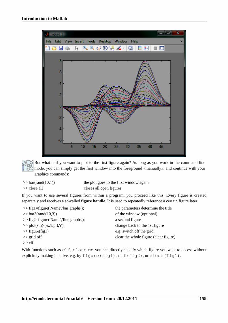
Introduction to Matlab
http://etools.fernuni.ch/matlab/ - Version from: 20.12.2011 159
But what is if you want to plot to the first figure again? As long as you work in the command linemode, you can simply get the first window into the foreground «manually», and continue with yourgraphics commands:
>> bar(rand(10,1))>> close all
the plot goes to the first window againcloses all open figures
If you want to use several figures from within a program, you proceed like this: Every figure is createdseparately and receives a so-called figure handle. It is used to repeatedly reference a certain figure later.
>> fig1=figure('Name','bar graphs');>> bar3(rand(10,3))>> fig2=figure('Name','line graphs');>> plot(sin(-pi:.1:pi),'r')>> figure(fig1)>> grid off>> clf
the parameters determine the titleof the window (optional)a second figurechange back to the 1st figuree.g. switch off the gridclear the whole figure (clear figure)
With functions such as clf, close etc. you can directly specify which figure you want to access withoutexplicitely making it active, e.g. by figure(fig1), clf(fig2), or close(fig1).
Introduction to Matlab
http://etools.fernuni.ch/matlab/ - Version from: 20.12.2011 160
Figure Properties
Changig the properties of figures is done with argument pairs, as you have seen inthe above example with the window title. The first argument of a pair indicates whichproperty you want to change (e.g. 'Name'), the second argument specifies the value tobe set.
For figures, a plethora of modifiable properties are available. You find the complete overview in the HelpSystem, for instance under the keyword 'figure properties' (docsearch 'figure properties').The most important ones are briefly described in the next section.The properties can either be set directly when creating a figure:>> fig2=figure('Name','line graphs');Or you can modify them later by means of set. For this, you need the handle of the figure to be modified.You can either specify the handle directly (that is, fig2), or you can recall the handle of the currently activefigure with gcf (get current figure). Example:>> set(fig2, 'Name', 'Another name');>> set(gcf, 'Name', 'Another name');
The most important figure properties'Name', 'titletext'Title of the figure window'Color', ColorSpecBackground colour. For information on how to specify colours see the Help System: doc colorspec.Examples:
>> set(gcf,'Color','yellow')>> set(gcf,'Color','r')>> set(gcf,'Color',[.8 .8 .8])
'yellow' is one of the pre-defined colours'r' is short for 'red'RGB colour triple, results in light gray
'Position', [left, bottom, width, height]Position and size of the windowleft, bottom: distance in pixels from the left and bottom screen borderwidth, height: width and height of the window in pixelsExample:>> fig=figure('Position', [100 100 800 600]);A useful assisting function: How to find out the screen size in case you want to size the window relative tothe screen size:>> ss=get(0,'ScreenSize')'Resize', 'on' or 'off'Determines whether the user can manually change the window size.'Toolbar', 'none' or 'auto'Determines whether the toolbar of the figure window is visible. 'auto' is the default value, that is, the windowis visible.'Visible', 'on' or 'off'With 'off', the window can be hidden, but it is still available for graphic outputs.
Introduction to Matlab
http://etools.fernuni.ch/matlab/ - Version from: 20.12.2011 161
Axes
Actually, a graphics output is not directed into a figure, but into the axes (or axes system) contained therein.An axes is - in Matlab terminology - a system of two (x, y) or three (x, y, z) axes. This should not be confusedwith axis, with which you can set the properties of the actual axis (e.g. the scales, see below).
Axes, too, have a multitude of properties (docsearch 'axes properties'), but'Color' is probably the only one you will ever use.
All other axes properties can be changed by separate commands. For a demonstration, please close allopen windows and create a new figure (simply use copy/paste):
>> close all>> figure('Position', [100 100 800 600])>> plot(peaks)Now we can change the settings:
>> title('Peaks function')>> grid off>> grid on>> axis off>> axis on>> axis([0 100 -20 20])>> axis tight>> set(gca,'Color','blue')
title of the graphswitch off the gridswitch it on againremove axis lineschange the scales: [xmin xmax ymin ymax]tightly fit the scales to the dataset background colour. gca = get current axes
Further options of axis: see the Help System doc axis
>> box on>> xlabel('Abscissa')>> ylabel('Ordinate')
box(frame) around the graphlabel the axes
Another useful function is Eine weitere nützliche Funktion ist waitforbuttonpress: It pauses programexecution until the user clicks into the graphics window or presses a key when the figure is active:>> figure, plot(peaks), waitforbuttonpress, bar(peaks)
A different method for user interaction: the figure property currentcharacter (see HelpSystem).
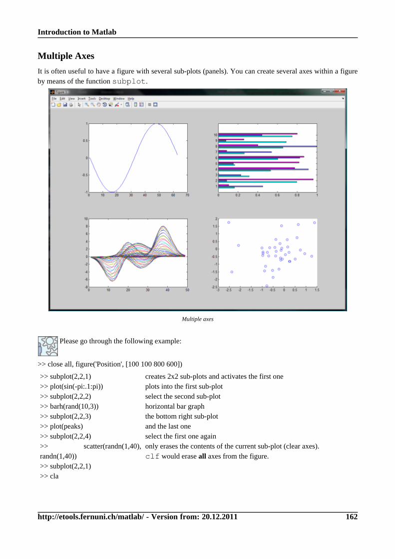
Introduction to Matlab
http://etools.fernuni.ch/matlab/ - Version from: 20.12.2011 162
Multiple Axes
It is often useful to have a figure with several sub-plots (panels). You can create several axes within a figureby means of the function subplot.
Multiple axes
Please go through the following example:
>> close all, figure('Position', [100 100 800 600])
>> subplot(2,2,1)>> plot(sin(-pi:.1:pi))>> subplot(2,2,2)>> barh(rand(10,3))>> subplot(2,2,3)>> plot(peaks)>> subplot(2,2,4)>> scatter(randn(1,40),randn(1,40))>> subplot(2,2,1)>> cla
creates 2x2 sub-plots and activates the first oneplots into the first sub-plotselect the second sub-plothorizontal bar graphthe bottom right sub-plotand the last oneselect the first one againonly erases the contents of the current sub-plot (clear axes).clf would erase all axes from the figure.
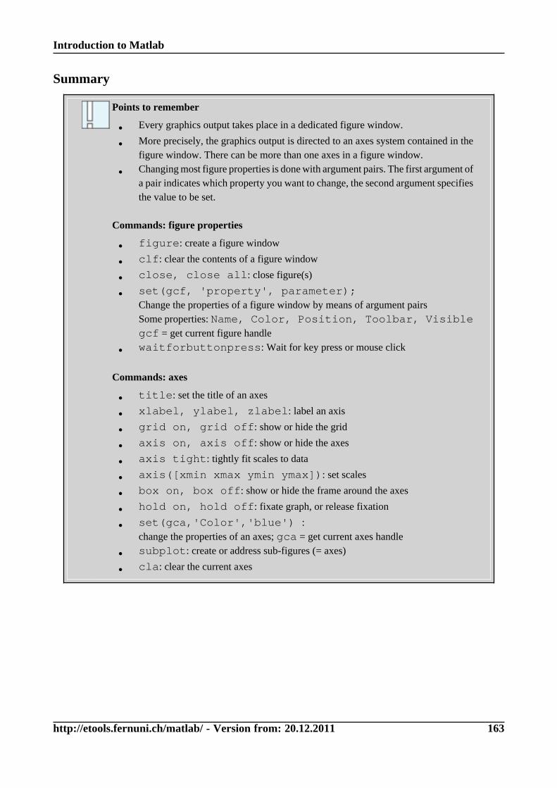
Introduction to Matlab
http://etools.fernuni.ch/matlab/ - Version from: 20.12.2011 163
Summary
Points to remember
• Every graphics output takes place in a dedicated figure window.
• More precisely, the graphics output is directed to an axes system contained in thefigure window. There can be more than one axes in a figure window.
• Changing most figure properties is done with argument pairs. The first argument ofa pair indicates which property you want to change, the second argument specifiesthe value to be set.
Commands: figure properties
• figure: create a figure window
• clf: clear the contents of a figure window
• close, close all: close figure(s)
• set(gcf, 'property', parameter);Change the properties of a figure window by means of argument pairsSome properties: Name, Color, Position, Toolbar, Visiblegcf = get current figure handle
• waitforbuttonpress: Wait for key press or mouse click
Commands: axes
• title: set the title of an axes
• xlabel, ylabel, zlabel: label an axis
• grid on, grid off: show or hide the grid
• axis on, axis off: show or hide the axes
• axis tight: tightly fit scales to data
• axis([xmin xmax ymin ymax]): set scales
• box on, box off: show or hide the frame around the axes
• hold on, hold off: fixate graph, or release fixation
• set(gca,'Color','blue') :change the properties of an axes; gca = get current axes handle
• subplot: create or address sub-figures (= axes)
• cla: clear the current axes
Introduction to Matlab
http://etools.fernuni.ch/matlab/ - Version from: 20.12.2011 164
Graphics ToolsBelow, you will get to know some important graphics tools. Again: Matlab offers many options, and it is notpossible here to explain all of them. As usual, you find everything in the Help System.
An overview over all graphics commands is given in the Help System under Function reference >graphics > basic plots and graphs
With the function plot as an example, the principle of most graphics commands are explained. After that,other frequently used graph types are briefly demonstrated.
Introduction to Matlab
http://etools.fernuni.ch/matlab/ - Version from: 20.12.2011 165
The Plot function
The plot function creates two-dimensional line graphs. The data have to be given as column vecors. Thedata points are connected by a line in the sequence as they are found in the vectors.
In the following examples, you can see the two forms of the plot function:
Form 1: plot(Y)If only one vector is given as argument, the data are interpreted as Y values and plotted against their indexon the X axis.>> ydata = sin(-pi:.1:pi);>> plot(ydata)Form 2: plot(X, Y)If two vectors are given, they are interpreded as X and Y axis data.>> xdata = 20:39; ydata = rand(20, 1);>> plot(xdata, ydata)>> figure>> plot(sin(-pi:.1:pi), cos(-pi:.1:pi))
LineSpec: set the line propertiesplot(X1, Y1, LineSpec, ...)The plot function accepts one argument that allows to set three important properties of the curve:
• Line style specifier: the style of the line (standard, dotted, dashed etc.)
• Marker specifier: the style of the data point markers (dot, circle, triangle, star, etc.)
• Color specifier: the colour of the curve
Example: To plot data with a red, dashed line and crosses as data markers, write:plot(x, y, '--xr')
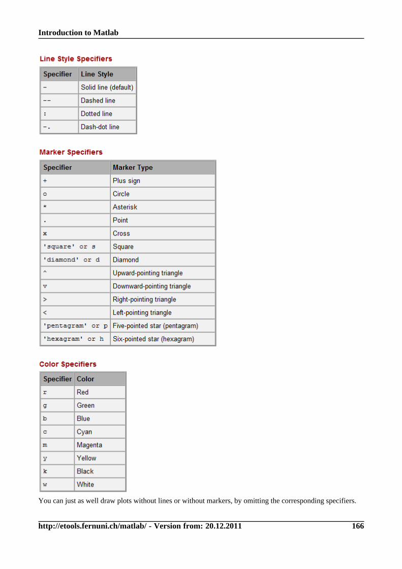
Introduction to Matlab
http://etools.fernuni.ch/matlab/ - Version from: 20.12.2011 166
You can just as well draw plots without lines or without markers, by omitting the corresponding specifiers.
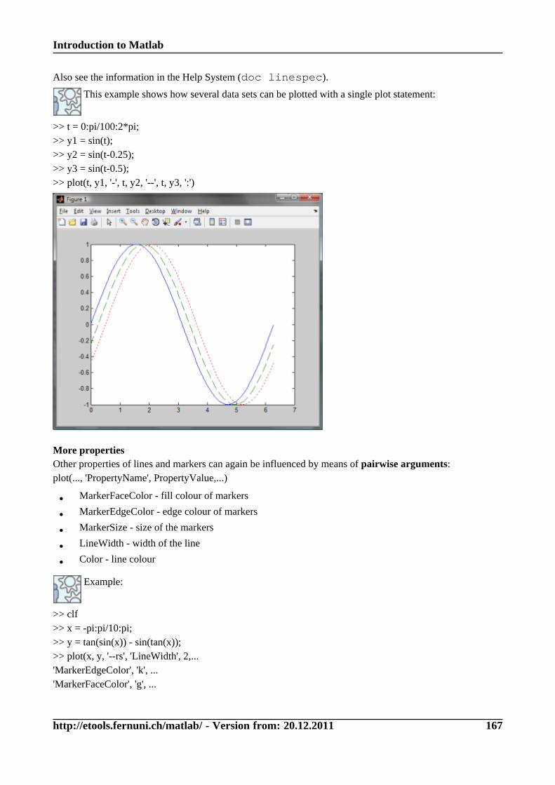
Introduction to Matlab
http://etools.fernuni.ch/matlab/ - Version from: 20.12.2011 167
Also see the information in the Help System (doc linespec).
This example shows how several data sets can be plotted with a single plot statement:
>> t = 0:pi/100:2*pi;>> y1 = sin(t);>> y2 = sin(t-0.25);>> y3 = sin(t-0.5);>> plot(t, y1, '-', t, y2, '--', t, y3, ':')
More propertiesOther properties of lines and markers can again be influenced by means of pairwise arguments:plot(..., 'PropertyName', PropertyValue,...)
• MarkerFaceColor - fill colour of markers
• MarkerEdgeColor - edge colour of markers
• MarkerSize - size of the markers
• LineWidth - width of the line
• Color - line colour
Example:
>> clf>> x = -pi:pi/10:pi;>> y = tan(sin(x)) - sin(tan(x));>> plot(x, y, '--rs', 'LineWidth', 2,...'MarkerEdgeColor', 'k', ...'MarkerFaceColor', 'g', ...
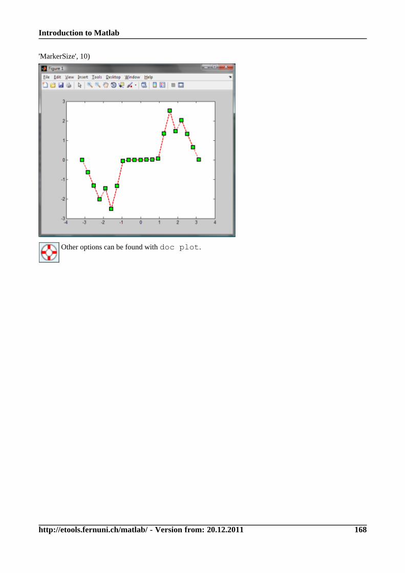
Introduction to Matlab
http://etools.fernuni.ch/matlab/ - Version from: 20.12.2011 168
'MarkerSize', 10)
Other options can be found with doc plot.
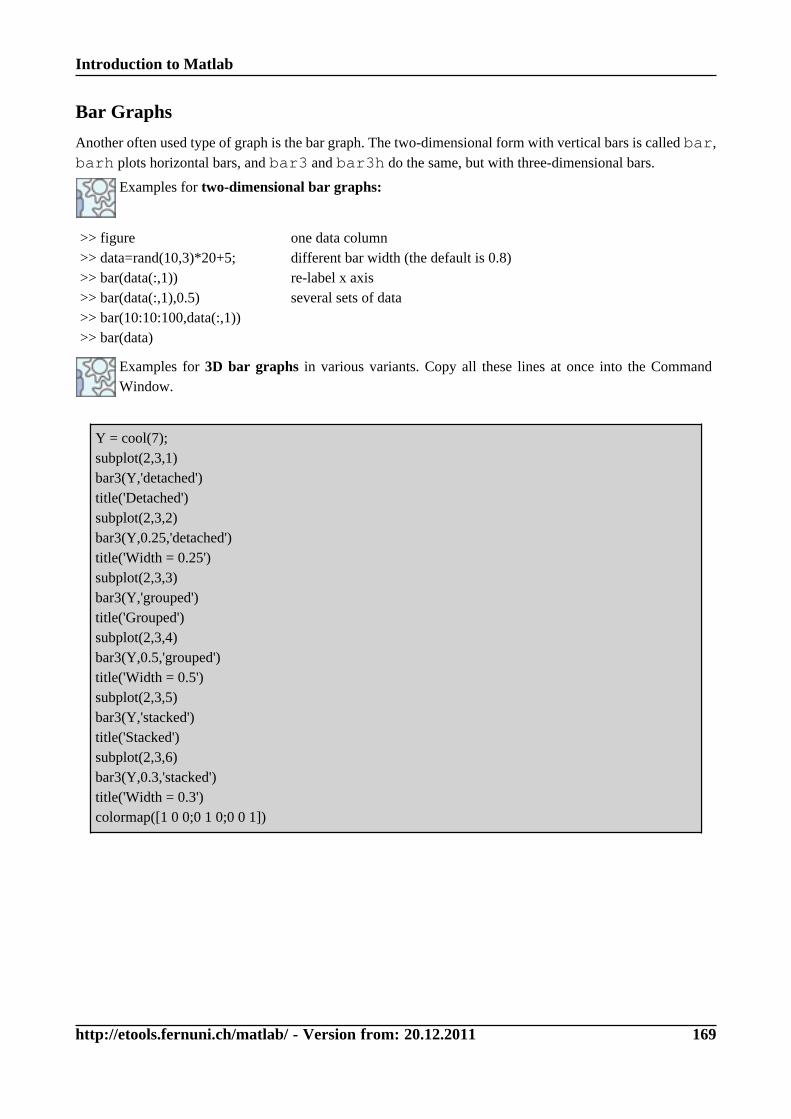
Introduction to Matlab
http://etools.fernuni.ch/matlab/ - Version from: 20.12.2011 169
Bar Graphs
Another often used type of graph is the bar graph. The two-dimensional form with vertical bars is called bar,barh plots horizontal bars, and bar3 and bar3h do the same, but with three-dimensional bars.
Examples for two-dimensional bar graphs:
>> figure>> data=rand(10,3)*20+5;>> bar(data(:,1))>> bar(data(:,1),0.5)>> bar(10:10:100,data(:,1))>> bar(data)
one data columndifferent bar width (the default is 0.8)re-label x axisseveral sets of data
Examples for 3D bar graphs in various variants. Copy all these lines at once into the CommandWindow.
Y = cool(7);subplot(2,3,1)bar3(Y,'detached')title('Detached')subplot(2,3,2)bar3(Y,0.25,'detached')title('Width = 0.25')subplot(2,3,3)bar3(Y,'grouped')title('Grouped')subplot(2,3,4)bar3(Y,0.5,'grouped')title('Width = 0.5')subplot(2,3,5)bar3(Y,'stacked')title('Stacked')subplot(2,3,6)bar3(Y,0.3,'stacked')title('Width = 0.3')colormap([1 0 0;0 1 0;0 0 1])
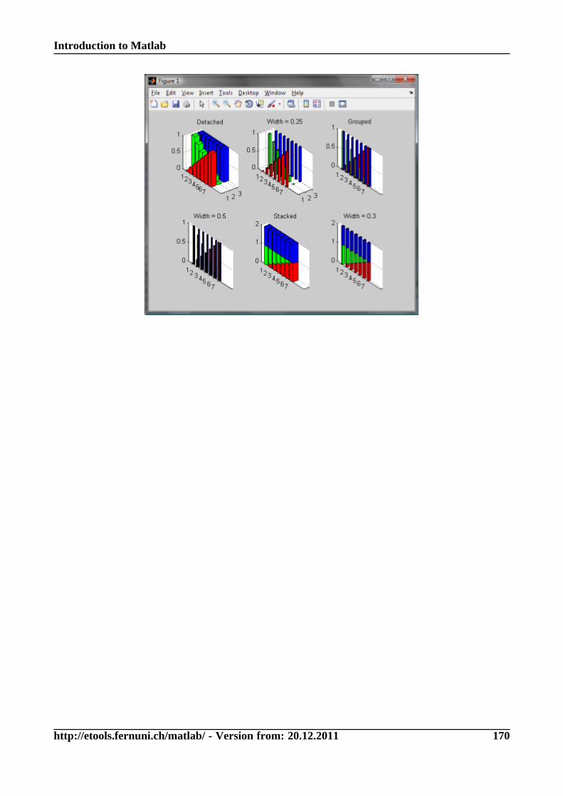
Introduction to Matlab
http://etools.fernuni.ch/matlab/ - Version from: 20.12.2011 170
Introduction to Matlab
http://etools.fernuni.ch/matlab/ - Version from: 20.12.2011 171
Brief Demonstration of Other Functions
Below, a script is used to illustrate some more of Matlab's interesting graphics options.
Please go to the Matlab Editor, load the script graph_examples.m and run it by hitting the F5 key.With a key press or mouse click into the figure window (function waitforbuttonpress) youcan continue to the next graph.
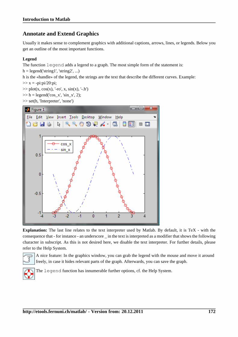
Introduction to Matlab
http://etools.fernuni.ch/matlab/ - Version from: 20.12.2011 172
Annotate and Extend Graphics
Usually it makes sense to complement graphics with additional captions, arrows, lines, or legends. Below youget an outline of the most important functions.
LegendThe function legend adds a legend to a graph. The most simple form of the statement is:h = legend('string1', 'string2', ...)h is the «handle» of the legend, the strings are the text that describe the different curves. Example:>> x = -pi:pi/20:pi;>> plot(x, cos(x), '-ro', x, sin(x), '-.b')>> h = legend('cos_x', 'sin_x', 2);>> set(h, 'Interpreter', 'none')
Explanation: The last line relates to the text interpreter used by Matlab. By default, it is TeX - with theconsequence that - for instance - an underscore _ in the text is interpreted as a modifier that shows the followingcharacter in subscript. As this is not desired here, we disable the text interpreter. For further details, pleaserefer to the Help System.
A nice feature: In the graphics window, you can grab the legend with the mouse and move it aroundfreely, in case it hides relevant parts of the graph. Afterwards, you can save the graph.
The legend function has innumerable further options, cf. the Help System.
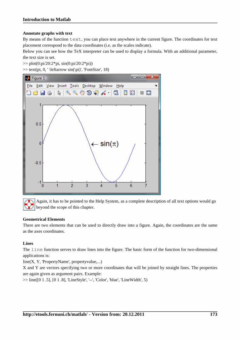
Introduction to Matlab
http://etools.fernuni.ch/matlab/ - Version from: 20.12.2011 173
Annotate graphs with textBy means of the function text, you can place text anywhere in the current figure. The coordinates for textplacement correspond to the data coordinates (i.e. as the scales indicate).Below you can see how the TeX interpreter can be used to display a formula. With an additional parameter,the text size is set.>> plot(0:pi/20:2*pi, sin(0:pi/20:2*pi))>> text(pi, 0, ' \leftarrow sin(\pi)', 'FontSize', 18)
Again, it has to be pointed to the Help System, as a complete description of all text options would gobeyond the scope of this chapter.
Geometrical ElementsThere are two elements that can be used to directly draw into a figure. Again, the coordinates are the sameas the axes coordinates.
LinesThe line function serves to draw lines into the figure. The basic form of the function for two-dimensionalapplications is:line(X, Y, 'PropertyName', propertyvalue,...)X and Y are vectors specifying two or more coordinates that will be joined by straight lines. The propertiesare again given as argument pairs. Example:>> line([0 1 .5], [0 1 .8], 'LineStyle', '--', 'Color', 'blue', 'LineWidth', 5)
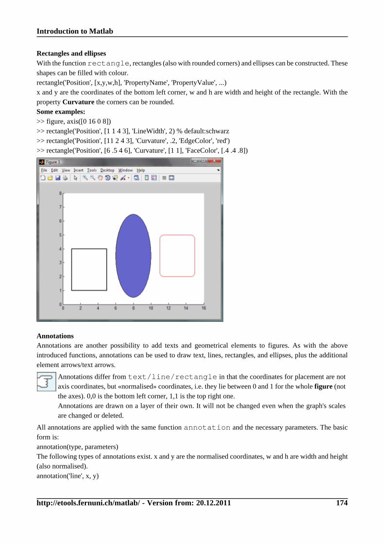
Introduction to Matlab
http://etools.fernuni.ch/matlab/ - Version from: 20.12.2011 174
Rectangles and ellipsesWith the function rectangle, rectangles (also with rounded corners) and ellipses can be constructed. Theseshapes can be filled with colour.rectangle('Position', [x,y,w,h], 'PropertyName', 'PropertyValue', ...)x and y are the coordinates of the bottom left corner, w and h are width and height of the rectangle. With theproperty Curvature the corners can be rounded.Some examples:>> figure, axis([0 16 0 8])>> rectangle('Position', [1 1 4 3], 'LineWidth', 2) % default:schwarz>> rectangle('Position', [11 2 4 3], 'Curvature', .2, 'EdgeColor', 'red')>> rectangle('Position', [6 .5 4 6], 'Curvature', [1 1], 'FaceColor', [.4 .4 .8])
AnnotationsAnnotations are another possibility to add texts and geometrical elements to figures. As with the aboveintroduced functions, annotations can be used to draw text, lines, rectangles, and ellipses, plus the additionalelement arrows/text arrows.
Annotations differ from text/line/rectangle in that the coordinates for placement are notaxis coordinates, but «normalised» coordinates, i.e. they lie between 0 and 1 for the whole figure (notthe axes). 0,0 is the bottom left corner, 1,1 is the top right one.Annotations are drawn on a layer of their own. It will not be changed even when the graph's scalesare changed or deleted.
All annotations are applied with the same function annotation and the necessary parameters. The basicform is:annotation(type, parameters)The following types of annotations exist. x and y are the normalised coordinates, w and h are width and height(also normalised).annotation('line', x, y)
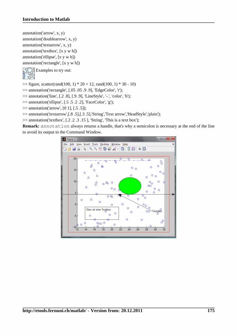
Introduction to Matlab
http://etools.fernuni.ch/matlab/ - Version from: 20.12.2011 175
annotation('arrow', x, y)annotation('doublearrow', x, y)annotation('textarrow', x, y)annotation('textbox', [x y w h])annotation('ellipse', [x y w h])annotation('rectangle', [x y w h])
Examples to try out:
>> figure, scatter(rand(100, 1) * 20 + 12, rand(100, 1) * 30 - 10)>> annotation('rectangle', [.05 .05 .9 .9], 'EdgeColor', 'r');>> annotation('line', [.2 .8], [.9 .9], 'LineStyle', '-.', 'color', 'b');>> annotation('ellipse', [.5 .5 .2 .2], 'FaceColor', 'g');>> annotation('arrow', [0 1], [.5 .5]);>> annotation('textarrow',[.8 .5],[.3 .5],'String','Text arrow','HeadStyle','plain');>> annotation('textbox', [.2 .2 .3 .15 ], 'String', 'This is a text box');Remark: annotation always returns a handle, that's why a semicolon is necessary at the end of the lineto avoid its output to the Command Window.
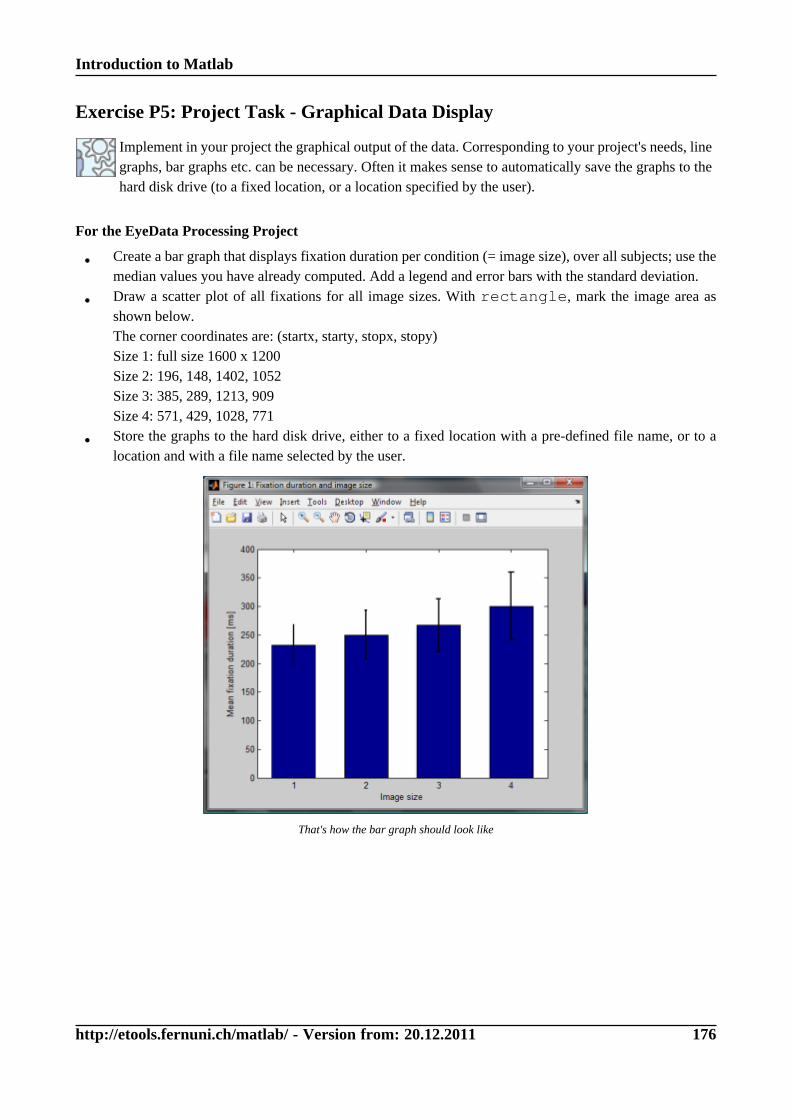
Introduction to Matlab
http://etools.fernuni.ch/matlab/ - Version from: 20.12.2011 176
Exercise P5: Project Task - Graphical Data Display
Implement in your project the graphical output of the data. Corresponding to your project's needs, linegraphs, bar graphs etc. can be necessary. Often it makes sense to automatically save the graphs to thehard disk drive (to a fixed location, or a location specified by the user).
For the EyeData Processing Project
• Create a bar graph that displays fixation duration per condition (= image size), over all subjects; use themedian values you have already computed. Add a legend and error bars with the standard deviation.
• Draw a scatter plot of all fixations for all image sizes. With rectangle, mark the image area asshown below.The corner coordinates are: (startx, starty, stopx, stopy)Size 1: full size 1600 x 1200Size 2: 196, 148, 1402, 1052Size 3: 385, 289, 1213, 909Size 4: 571, 429, 1028, 771
• Store the graphs to the hard disk drive, either to a fixed location with a pre-defined file name, or to alocation and with a file name selected by the user.
That's how the bar graph should look like
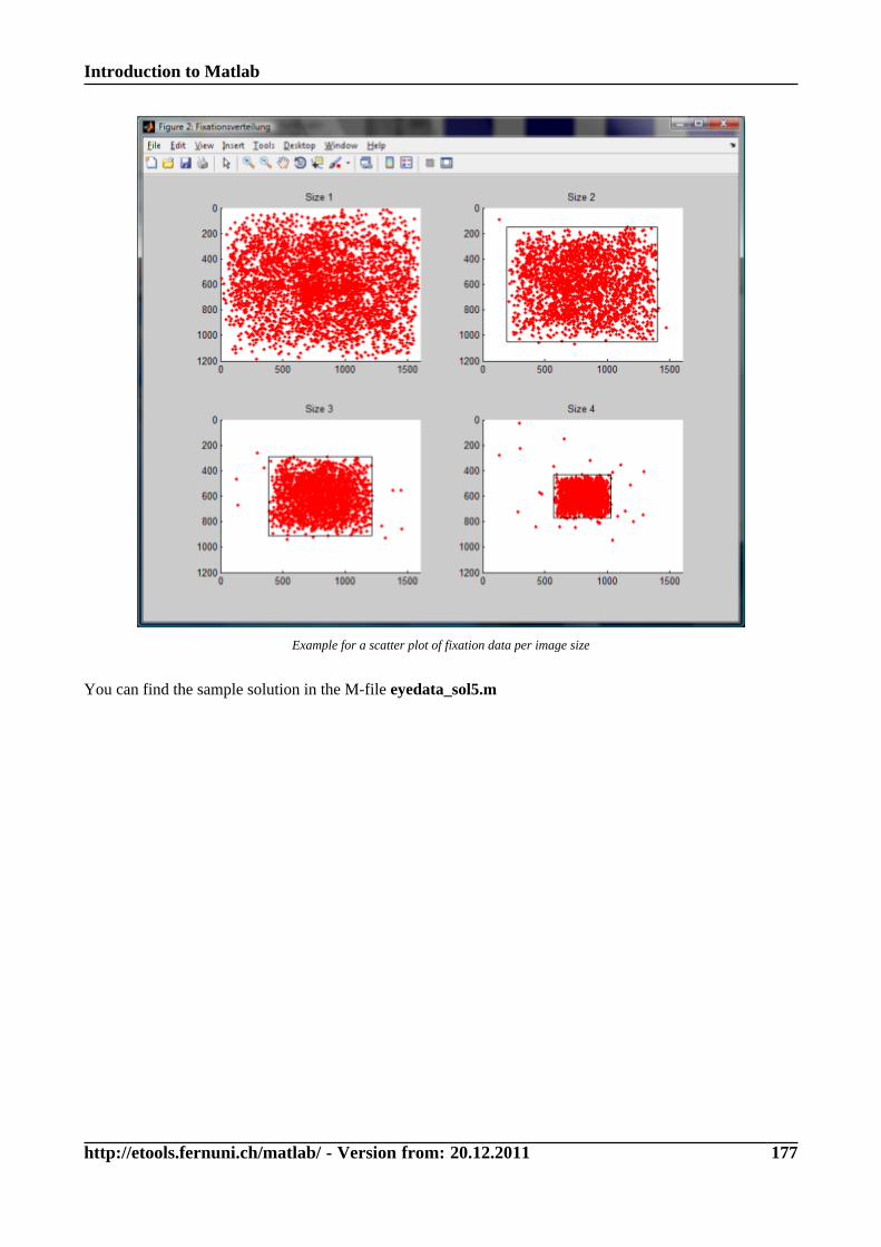
Introduction to Matlab
http://etools.fernuni.ch/matlab/ - Version from: 20.12.2011 177
Example for a scatter plot of fixation data per image size
You can find the sample solution in the M-file eyedata_sol5.m
Introduction to Matlab
http://etools.fernuni.ch/matlab/ - Version from: 20.12.2011 178
Summary
Summary of the most important commands:
• plot: plot data
• bar, barh, bar3, bar3h: bar graphs; normal, horizontal, and 3D, 3Dhorizontal.
• legend: show the legend
• text, line, rectangle: draw texts, lines, or rectangles (and ellipses)in the current axes of a figure
• annotation: draw graphical elements in relative (normalised) coordinates ofthe whole figure,e.g. annotation('rectangle', [.05 .05 .9 .9], 'EdgeColor', 'r');
Introduction to Matlab
http://etools.fernuni.ch/matlab/ - Version from: 20.12.2011 179
Final RemarksYou have now reached the end of this course. We hope that it has helped you to start with Matlab. We arefully aware that learning a new programming language is a very demanding undertaking - especially if youare new to programming.
Only pictures can be viewed in this version! For Flash, animations, movies etc. see online version.Only screenshots of animations will be displayed. [link]
Thus, we are very much interested in improving this course. If you have any comments, suggestions, or if youhave found errors, please let us know!
If you would like to support our initiative to build this course, which is an openeducational resource, and are a native speaker of English: The course is in need ofproofreading, as it was translated by a non-native speaker of English (as you sure havenoticed).If you are willing to proofread a part (however small) of this course, please contact me.Thank you very much!