Introduction to MATLAB

Markus Kuhn

Computer Laboratory, University of Cambridge

https://www.cl.cam.ac.uk/teaching/1718/TeX+MATLAB/

MathWorks Logo

matlab-slides.pdf 2017-10-27 12:55 f3394f3 1 / 20

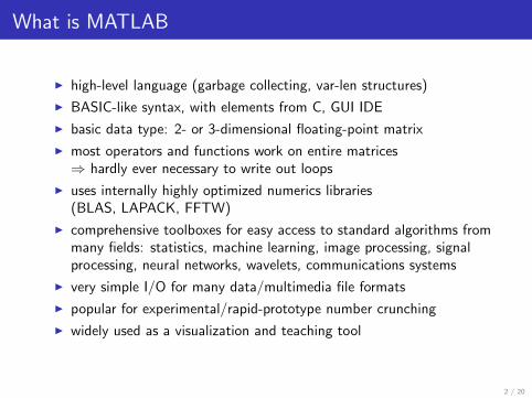
What is MATLAB

I high-level language (garbage collecting, var-len structures)

I BASIC-like syntax, with elements from C, GUI IDE

I basic data type: 2- or 3-dimensional floating-point matrix

I most operators and functions work on entire matrices⇒ hardly ever necessary to write out loops

I uses internally highly optimized numerics libraries(BLAS, LAPACK, FFTW)

I comprehensive toolboxes for easy access to standard algorithms frommany fields: statistics, machine learning, image processing, signalprocessing, neural networks, wavelets, communications systems

I very simple I/O for many data/multimedia file formats

I popular for experimental/rapid-prototype number crunching

I widely used as a visualization and teaching tool

2 / 20

What MATLAB is not

I not a computer algebra system

I not a strong general purpose programming language

• limited support for other data structures

• few software-engineering features;typical MATLAB programs are only a few lines long

• not well-suited for teaching OOP

• limited GUI features

I not a high-performance language (but fast matrix operators)got better since introduction of JIT compiler (JVM)

I not freely available (but local campus licence)

3 / 20

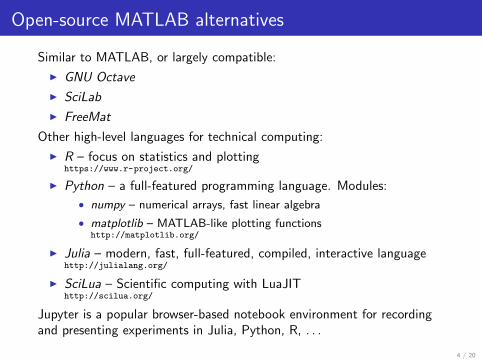
Open-source MATLAB alternatives

Similar to MATLAB, or largely compatible:

I GNU Octave

I SciLab

I FreeMat

Other high-level languages for technical computing:

I R – focus on statistics and plottinghttps://www.r-project.org/

I Python – a full-featured programming language. Modules:

• numpy – numerical arrays, fast linear algebra

• matplotlib – MATLAB-like plotting functionshttp://matplotlib.org/

I Julia – modern, fast, full-featured, compiled, interactive languagehttp://julialang.org/

I SciLua – Scientific computing with LuaJIThttp://scilua.org/

Jupyter is a popular browser-based notebook environment for recordingand presenting experiments in Julia, Python, R, . . .

4 / 20

Local availability

MATLAB is installed and ready to use on

I Intel Lab, etc.: MCS Windows

I Intel Lab, etc.: MCS Linux (/usr/bin/matlab)

I CL MCS Linux server: ssh -X linux.cl.ds.cam.ac.uk

I MCS Linux server: ssh -X linux.ds.cam.ac.uk

I Computer Laboratory managed Linux PCscl-matlab -> /usr/groups/matlab/current/bin/matlab

Campus license allows installation on staff/student home PCs(Linux, macOS, Windows):

I https://help.uis.cam.ac.uk/devices-networks-printing/

compsoft/matlab

I Includes toolboxes for Statistics and Machine Learning, SignalProcessing, Image Processing, Bioinformatics, Control Systems,Wavelets, . . .

I Installation requires setting up a http://uk.mathworks.com/

account with your @cam.ac.uk email address.

Computer Laboratory researchers can access additional toolboxes:

I https://www.cl.cam.ac.uk/local/sys/resources/matlab/5 / 20

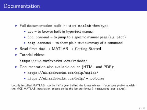
Documentation

I Full documentation built in: start matlab then type

• doc – to browse built-in hypertext manual

• doc command – to jump to a specific manual page (e.g. plot)

• help command – to show plain-text summary of a command

I Read first: doc → MATLAB → Getting Started

I Tutorial videos:

https://uk.mathworks.com/videos/

I Documentation also available online (HTML and PDF):

• https://uk.mathworks.com/help/matlab/

• https://uk.mathworks.com/help/ – toolboxes

Locally installed MATLAB may be half a year behind the latest release. If you spot problems withthe MCS MATLAB installation, please do let the lecturer know (→ mgk25@cl.cam.ac.uk).

6 / 20

MATLAB matrices (1)

Generate a “magic square” with equal row/column/diagonal sums andassign the resulting 3× 3 matrix to variable a:

>> a = magic(3)

a =

8 1 6

3 5 7

4 9 2

Assignments and subroutine calls normally end with a semicolon.

Without, MATLAB will print each result. Useful for debugging!

Results from functions not called inside an expression are assigned to thedefault variable ans.

Type help magic for the manual page of this library function.

7 / 20

MATLAB matrices (2)

Colon generates number sequence:

>> 11:14

ans =

11 12 13 14

>> -1:1

ans =

-1 0 1

>> 3:0

ans =

Empty matrix: 1-by-0

Specify step size with second colon:

>> 1:3:12

ans =

1 4 7 10

>> 4:-1:1

ans =

4 3 2 1

>> 3:-0.5:2

ans =

3.0000 2.5000 2.0000

Single matrix cell: a(2,3) == 7. Vectors as indices select several rows andcolumns. When used inside a matrix index, the variable end provides thehighest index value: a(end, end-1) == 9. Using just “:” is equivalent to“1:end” and can be used to select an entire row or column.

8 / 20

MATLAB matrices (3)

Select rows, columns andsubmatrices of a:

>> a(1,:)

ans =

8 1 6

>> a(:,1)

ans =

8

3

4

>> a(2:3,1:2)

ans =

3 5

4 9

Matrices can also be accessed as a1-dimensional vector:

>> a(1:5)

ans =

8 3 4 1 5

>> a(6:end)

ans =

9 6 7 2

>> b = a(1:4:9)

ans =

8 5 2

>> size(b)

ans =

1 3

9 / 20

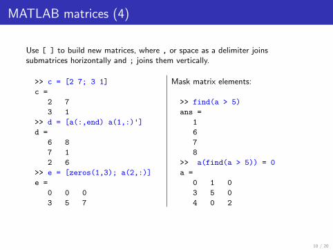
MATLAB matrices (4)

Use [ ] to build new matrices, where , or space as a delimiter joinssubmatrices horizontally and ; joins them vertically.

>> c = [2 7; 3 1]

c =

2 7

3 1

>> d = [a(:,end) a(1,:)']

d =

6 8

7 1

2 6

>> e = [zeros(1,3); a(2,:)]

e =

0 0 0

3 5 7

Mask matrix elements:

>> find(a > 5)

ans =

1

6

7

8

>> a(find(a > 5)) = 0

a =

0 1 0

3 5 0

4 0 2

10 / 20

Review: matrix multiplication

• • • •• • • •• • • •

· ‖

• • •• • •• • •• • •• • •

·

• • • •• • • •• • • •

=

• • • •• • • •• • • •• • • •• • • •

Each element of the matrix product is the scalar product ofthe corresponding row in the first factor andthe corresponding column in the second factor

11 / 20

Review: matrix multiplication

• • • •• • • •• • • •

·

‖

• • •• • •• • •• • •• • •

·

=

• • • •• • • •• • • •• • • •• • • •

Each element of the matrix product is the scalar product ofthe corresponding row in the first factor andthe corresponding column in the second factor

11 / 20

Review: matrix multiplication

• • • •• • • •• • • •

· ‖

• • •• • •• • •• • •• • •

·

• • • •• • • •• • • •• • • •• • • •

=

• • • •• • • •• • • •• • • •• • • •

Each element of the matrix product is the scalar product ofthe corresponding row in the first factor andthe corresponding column in the second factor

11 / 20

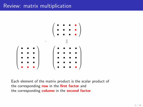
Review: matrix multiplication

• • • •• • • •• • • •

· ‖

• • •• • •• • •• • •• • •

·

• • • •• • • •• • • •• • • •• • • •

=

• • • •• • • •• • • •• • • •• • • •

Each element of the matrix product is the scalar product ofthe corresponding row in the first factor andthe corresponding column in the second factor

11 / 20

Review: matrix multiplication

• • • •• • • •• • • •

· ‖

• • •• • •• • •• • •• • •

·

• • • •• • • •• • • •• • • •• • • •

=

• • • •• • • •• • • •• • • •• • • •

Each element of the matrix product is the scalar product ofthe corresponding row in the first factor andthe corresponding column in the second factor

11 / 20

Review: matrix multiplication

• • • •• • • •• • • •

· ‖

• • •• • •• • •• • •• • •

·

• • • •• • • •• • • •• • • •• • • •

=

• • • •• • • •• • • •• • • •• • • •

Each element of the matrix product is the scalar product ofthe corresponding row in the first factor andthe corresponding column in the second factor

11 / 20

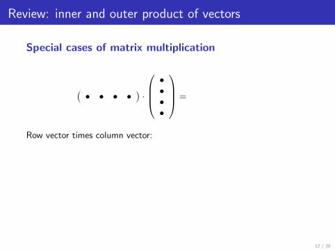
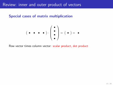
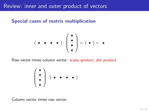
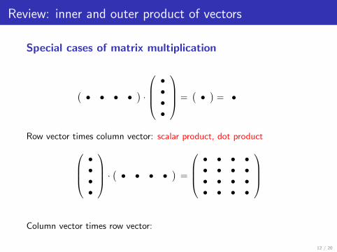
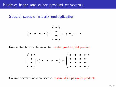
Review: inner and outer product of vectors

Special cases of matrix multiplication

(• • • •

)·

••••

=

(•)

= •

Row vector times column vector:

scalar product, dot product••••

· ( • • • •)

=

• • • •• • • •• • • •• • • •

Column vector times row vector:

matrix of all pair-wise products

12 / 20

Review: inner and outer product of vectors

Special cases of matrix multiplication

(• • • •

)·

••••

=(•)

= •

Row vector times column vector:

scalar product, dot product••••

· ( • • • •)

=

• • • •• • • •• • • •• • • •

Column vector times row vector:

matrix of all pair-wise products

12 / 20

Review: inner and outer product of vectors

Special cases of matrix multiplication

(• • • •

)·

••••

=(•)

= •

Row vector times column vector: scalar product, dot product

••••

· ( • • • •)

=

• • • •• • • •• • • •• • • •

Column vector times row vector:

matrix of all pair-wise products

12 / 20

Review: inner and outer product of vectors

Special cases of matrix multiplication

(• • • •

)·

••••

=(•)

= •

Row vector times column vector: scalar product, dot product••••

· ( • • • •)

=

• • • •• • • •• • • •• • • •

Column vector times row vector:

matrix of all pair-wise products

12 / 20

Review: inner and outer product of vectors

Special cases of matrix multiplication

(• • • •

)·

••••

=(•)

= •

Row vector times column vector: scalar product, dot product••••

· ( • • • •)

=

• • • •• • • •• • • •• • • •

Column vector times row vector:

matrix of all pair-wise products

12 / 20

Review: inner and outer product of vectors

Special cases of matrix multiplication

(• • • •

)·

••••

=(•)

= •

Row vector times column vector: scalar product, dot product••••

· ( • • • •)

=

• • • •• • • •• • • •• • • •

Column vector times row vector: matrix of all pair-wise products

12 / 20

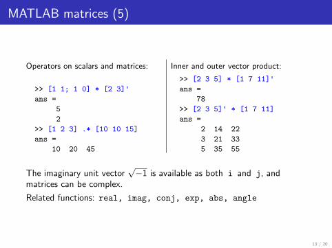
MATLAB matrices (5)

Operators on scalars and matrices:

>> [1 1; 1 0] * [2 3]'

ans =

5

2

>> [1 2 3] .* [10 10 15]

ans =

10 20 45

Inner and outer vector product:

>> [2 3 5] * [1 7 11]'

ans =

78

>> [2 3 5]' * [1 7 11]

ans =

2 14 22

3 21 33

5 35 55

The imaginary unit vector√−1 is available as both i and j, and

matrices can be complex.

Related functions: real, imag, conj, exp, abs, angle

13 / 20

Plotting

0 5 10 15 20

0

0.2

0.4

0.6

0.8

120-point raised cosine

x = 0:20;y = 0.5 - 0.5*cos(2*pi * x/20);stem(x, y);title('20-point raised cosine');

0 2 4 6 8 10-0.4

-0.2

0

0.2

0.4

0.6

0.8

1

real

imaginary

t = 0:0.1:10;x = exp(t * (j - 1/3));plot(t, real(x), t, imag(x));grid; legend('real', 'imaginary')

Plotting functions plot, semilogx, semilogy, loglog all expect a pair ofvectors for each curve, with x and y coordinates, respectively.

Use saveas(gcf, 'plot2.eps') to save current figure as graphics file.

14 / 20

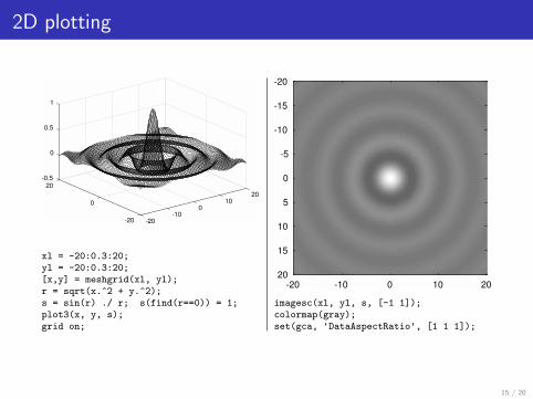
2D plotting

-0.5

20

0

20

0.5

100

1

0

-10-20 -20

xl = -20:0.3:20;yl = -20:0.3:20;[x,y] = meshgrid(xl, yl);r = sqrt(x.^2 + y.^2);s = sin(r) ./ r; s(find(r==0)) = 1;plot3(x, y, s);grid on;

-20 -10 0 10 20

-20

-15

-10

-5

0

5

10

15

20

imagesc(xl, yl, s, [-1 1]);colormap(gray);set(gca, 'DataAspectRatio', [1 1 1]);

15 / 20

Some common functions and operators

*, ^matrix multiplication, exponentiation

/, \, invA/B = AB−1, A\B = A−1B, A−1

+, -, .*, ./, .^element-wise add/sub/mul/div/exp

==, ~=, <, >, <=, >=relations result in element-wise 0/1

length, sizesize of vectors and matrices

zeros, ones, eye, diagall-0, all-1, identity, diag. matrices

xlim, ylim, zlimset plot axes ranges

xlabel, ylabel, zlabellabel plot axes

audioread, audiowrite, soundaudio I/O

csvread, csvwritecomma-separated-value I/O

imread, imwrite, image,

imagesc, colormapbitmap image I/O

plot, semilog{x,y}, loglog2D curve plotting

conv, conv2, xcorr1D/2D convolution,cross/auto-correlation sequence

fft, ifft, fft2discrete Fourier transform

sum, prod, min, maxsum up rows or columns

cumsum, cumprod, diffcumulative sum or product,differentiate row/column

findlist non-zero indices

figure, saveasopen new figure, save figure

16 / 20

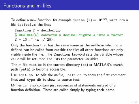
Functions and m-files

To define a new function, for example decibel(x) = 10x/20, write into afile decibel.m the lines

function f = decibel(x)

% DECIBEL(X) converts a decibel figure X into a factor

f = 10 .^ (x ./ 20);

Only the function that has the same name as the m-file in which it isdefined can be called from outside the file; all other functions are onlyvisible inside the file. The function keyword sets the variable whosevalue will be returned and lists the parameter variables.

The m-file must be in the current directory (cd) or MATLAB’s searchpath (path) to become accessible.

Use edit db to edit the m-file, help db to show the first commentlines and type db to show its source text.

M-files can also contain just sequences of statements instead of afunction definition. These are called simply by typing their name.

17 / 20

Example: generating an audio illusion

Generate an audio file with 12 sine tones of apparently continuouslyexponentially increasing frequency, which never leave the frequency range300–3400 Hz. Do this by letting them wrap around the frequency intervaland reduce their volume near the interval boundaries based on araised-cosine curve applied to the logarithm of the frequency.

First produce a 2 s long waveform in which each tone raises 1/12 of thefrequency range, then concatenate that into a 60 s long 16-bit WAV file,mono, with 16 kHz sampling rate. Avoid phase jumps.

Parameters:

fs = 16000; % sampling frequency [Hz]

d = 2; % time after which waveform repeats [s]

n = 12; % number of tones

fmin = 300; % lowest frequency

fmax = 3400; % highest frequency

18 / 20

Spectrogram of the first 6 s:

1 2 3 4 5

Time

0

500

1000

1500

2000

2500

3000

3500F

requency

19 / 20

Example solution:t = 0:1/fs:d-1/fs; % timestamps for each sample point

% normalized logarithm of frequency of each tone (row)

% for each sample point (column), all rising linearly

% from 0 to 1, then wrap around back to 0

l = mod(((0:n-1)/n)' * ones(1, fs*d) + ones(n,1) * (t/(d*n)), 1);

f = fmin * (fmax/fmin) .^ l; % freq. for each tone and sample

p = 2*pi * cumsum(f, 2) / fs; % phase for each tone and sample

% make last column a multiple of 2*pi for phase continuity

p = diag((2*pi*floor(p(:,end)/(2*pi))) ./ p(:,end)) * p;

s = sin(p); % sine value for each tone and sample

% mixing amplitudes from raised-cosine curve over frequency

a = 0.5 - 0.5 * cos(2*pi * l);

w = sum(s .* a)/n; % mix tones together, normalize to [-1, +1]

w = repmat(w, 1, 3); % repeat waveform 3x

specgram(w, 2048, fs, 2048, 1800); ylim([0 fmax*1.1]) % plot

w = repmat(w, 1, 20); % repeat waveform 20x

audiowrite('ladder.wav', w, fs, 'BitsPerSample', 16); % make audio file

A variant of this audio effect, where each tone is exactly one octave (factor 2 in frequency) fromthe next, is known as the Shepard–Risset glissando.

What changes to the parameters would produce that?

20 / 20