Introduction to MATLAB MATLAB in Science, Engineering, and Mathematics Instruction John Sebeson DeVry University

Introduction to MATLAB

MATLAB in Science, Engineering, and Mathematics Instruction

John SebesonDeVry University

January 18, 2005 J. M. Sebeson - DeVry University © 2005

What is MATLAB? MATLAB stands for MATrix LABoratory. MATLAB is a high-performance language for

technical computing. Math and computation Algorithm development (optimized for DSP) Data acquisition Modeling, simulation, and prototyping Data analysis, exploration, and visualization Scientific and engineering graphics Application development, including graphical

user interface building


Why Learn and Use MATLAB? Heavily used in EET/CET courses with DSP

content (CET311, EET350, EET453) Extensive built-in commands for scientific

and engineering mathematics Easy way to generate class demonstrations

and test examples Simple and intuitive programming for more

complex problems Standard and widely-used computational

environment with many features, extensions, and links to other software.


MATLAB in DSP Product Development

Develop and Test Algorithms in MATLAB

SIMULINK Simulation

Code Composer

DSP Processor Platform

MATLAB + PC = DSP Processor!! (just less efficient)


Why Learn MATLAB (and DSP)? Digital Signal Processing (DSP) is the

dominant technology today, and into the future, for small-signal electronic systems (i.e., just about everything)

MATLAB has become one of the standard design environments for DSP engineering

Our students need to be literate and skilled in this environment: knowledgeable in both DSP and MATLAB


How Can I Learn MATLAB? Keep a copy of this presentation for

reference (available on my Web Page)

Get MATLAB loaded on your PC Read the “Getting Started” Users

Guide at the MathWorks web site Study some of the built-in help files

and demos Dive right in and use it!


This Presentation The MATLAB System The basics of MATLAB computation The basics of MATLAB graphing The basics of MATLAB programming Various course examples

Mathematics Electronics Physics Signal Processing(*)


The MATLAB System Development Environment.

MATLAB desktop Editor and debugger for MATLAB programs (“m-files”) Browsers for help, built-in and on-line documentation Extensive demos

The MATLAB Mathematical Function Library. Elementary functions, like sum, sine, cosine, and complex arithmetic More sophisticated functions like matrix inverse, matrix eigenvalues, Bessel

functions, and fast Fourier transforms. “Toolboxes” for special application areas such as Signal Processing

The MATLAB Language. “Programming in the small" to rapidly create quick and dirty throw-away programs,

or “Programming in the large" to create large and complex application programs.

Graphics. 2D and 3D plots Editing and annotation features

The MATLAB Application Program Interface (API). A library that allows you to write C and Fortran programs that interact with

MATLAB.


MATLAB Development Environment (Workspace)


MATLAB “Help” Utilities MATLAB is so rich that ‘help’ is essential

Command name and syntax Command input/output parameters Usage examples

Help command help command_name help [partial_name] tab

Help documents Demos


MATLAB Function Library (A Subset)

matlab\general - General purpose commands.matlab\ops - Operators and special characters.matlab\lang - Programming language constructs.matlab\elmat - Elementary matrices and matrix manipulation.matlab\elfun - Elementary math functions.matlab\specfun - Specialized math functions.matlab\matfun - Matrix functions - numerical linear algebra.matlab\datafun - Data analysis and Fourier transforms.matlab\polyfun - Interpolation and polynomials.matlab\funfun - Function functions and ODE solvers.matlab\sparfun - Sparse matrices.matlab\scribe - Annotation and Plot Editing.matlab\graph2d - Two dimensional graphs.matlab\graph3d - Three dimensional graphs.matlab\specgraph - Specialized graphs.matlab\graphics - Handle Graphics.


Some Elementary Functions

Exponential.

exp - Exponential. expm1 - Compute exp(x)-1 accurately. log - Natural logarithm. log1p - Compute log(1+x) accurately. log10 - Common (base 10) logarithm. log2 - Base 2 logarithm and dissect floating point number. pow2 - Base 2 power and scale floating point number. realpow - Power that will error out on complex result. reallog - Natural logarithm of real number. realsqrt - Square root of number greater than or equal to zero. sqrt - Square root. nthroot - Real n-th root of real numbers. nextpow2 - Next higher power of 2.


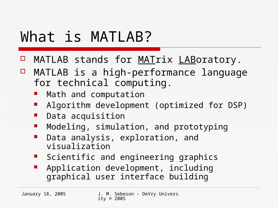
Some Specialized Functions

Number theoretic functions.

factor - Prime factors. isprime - True for prime numbers. primes - Generate list of prime numbers. gcd - Greatest common divisor. lcm - Least common multiple. rat - Rational approximation. rats - Rational output. perms - All possible permutations. nchoosek - All combinations of N elements taken K at a time. factorial - Factorial function.


The MATLAB Language (M-file example)

function one_period(amp,freq,phase)% ONE_PERIOD(AMP,FREQ,PHASE)% This function plots one period of a sine wave with a given amplitude,% frequency (in Hz), and phase ( in degrees).T=1000/freq; % Compute the period in mst=0:T/100:T; % Define a 100 point ms time vector 1 period longy=amp*sin(2*pi*t/T+phase*pi/180); % One period of the sine functionplot(t,y) % Plot the result and format the axes and titlexlabel('milliseconds')ylabel('amplitude')title(['One Period of a ',num2str(freq),' Hz Sinewave with ',num2str(phase), ' Degree phase'])


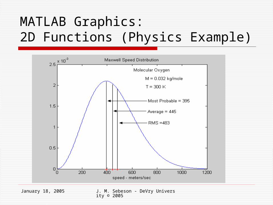
MATLAB Graphics:2D Functions (Physics Example)


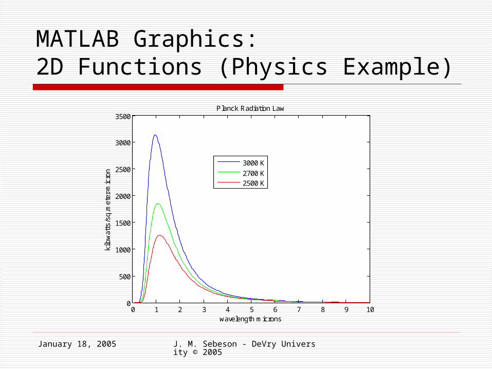
MATLAB Graphics:2D Functions (Physics Example)

0 1 2 3 4 5 6 7 8 9 100

500

1000

1500

2000

2500

3000

3500

wavelength microns

kilo

wat

ts/s

q.m

eter

-mic

ron

Planck Radiation Law

3000 K

2700 K2500 K


MATLAB Graphics:3D Functions (DSP Example)


Basic MATLAB Computation:Representation of Numbers and Variables

MATLAB operates on n row by m column matrices: A n x m quantity is an array

A 1 x m or a n x 1 quantity is a vector

[8 1 6]

A 1 x 1 quantity is a scalar[8]

[8 1 6 3 5 7 4 9 2]


Basic MATLAB Computation:Basic Operations

Array manipulation (Magic Square example) Sum, diag, transpose, colon operator,

indexing Array, vector, and scalar operators

Matrix and vector addition and multiplication

Element-by-element operations Variable statements and definitions


MATLAB Plotting and Graphics

Rich set of commands for 2D and 3D plotting of functions

Command formatting and editing GUI formatting and editing Image display capabilities Animation capabilities Simple “copy and paste” for

publishing generated figures


MATLAB PlottingBasic Commands plot – x,y line plots stem – n,y discrete plots (standard

representation of digital signals) bar – vertical bar plots plot3 – 3D x,y,z line plots mesh, surf, etc. – 3D surface plots show_img – display matrix as an image hold – hold current figure for multiple line plots subplot – put multiple plots in one figure frame Etc, etc. - See MATLAB help documentation


Basic Plotting - Examples Plot of sin(x) function Stem of sin(x) function Bar of sin(x) function Several sine functions with “hold” Several sine functions with “subplot” 2D plot of sinc(x) 3D plot of sinc(x) [“plot_sinc” m-file]

GUI editing View by rotation

Animation [“brownian_demo” m-file]


Basic MATLAB Programming Scripts

String of MATLAB commands Stored as m-file (*.m) Use variables from command line Variables have names consistent with script variable names Used for “quick and dirty” programs Example: “dydx_script”

Functions String of MATLAB commands Stored as m-file (*.m) Use variables as function parameters No restriction on parameter names Can return variable results Used for general purpose programs Example: “yy=dydx(x,y)


Structure of m-file Functions:Examples

“one_period” Use of “num2str” for variable formatting

“sumofsines” Use of parameter-controlled data input

loops “fft_plot”

Use of MATLAB functions as subroutines Use of “nargin” test and branch


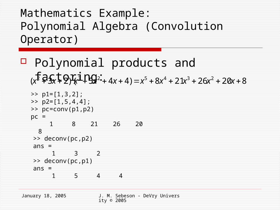
Mathematics Example:Polynomial Algebra (Convolution Operator)

Polynomial products and factoring:

82026218)445)(23( 2345232 xxxxxxxxxx

>> p1=[1,3,2];>> p2=[1,5,4,4];>> pc=conv(p1,p2)pc = 1 8 21 26 20 8

>> deconv(pc,p2)ans = 1 3 2>> deconv(pc,p1)ans = 1 5 4 4


Mathematics Example:Linear Systems Solve the system:

A*S=B MATLAB Code:

609

234

3325

zyx

zy

zyx

>> A=[5,-2,-3;0,4,3;1,-1,9];>> B=[-3,-2,60]'; % Note vector transpose (‘)>> S=linsolve(A,B)S = 1.0000 -5.0000 6.0000


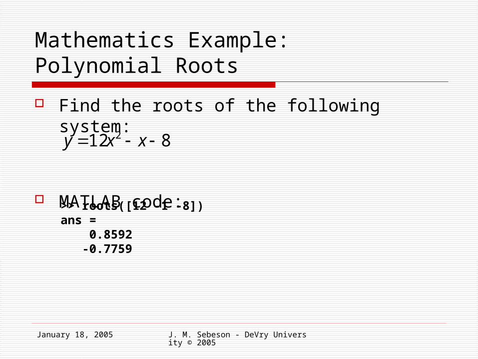
Mathematics Example:Polynomial Roots

Find the roots of the following system:

MATLAB code:

812 2 xxy

>> roots([12 -1 -8])ans = 0.8592 -0.7759


Mathematics Example:Polynomial Roots

Graphical Solution:

>> a=12;>> b=-1;>> c=-8;>> x=-1:0.1:1;>> y=a*x.^2+b*x+c;>> plot(x,y)


Electronic Circuits Example:Mesh Analysis (Linear System)

Find the currents in each branch: I1, I2

-7I1 + 6I2 = 5

6I1 – 8I2 = -10

>> A=[-7,6;6,-8];>> B=[5;-10];>> X=linsolve(A,B)ans = 1.0000 2.0000

A*X = B


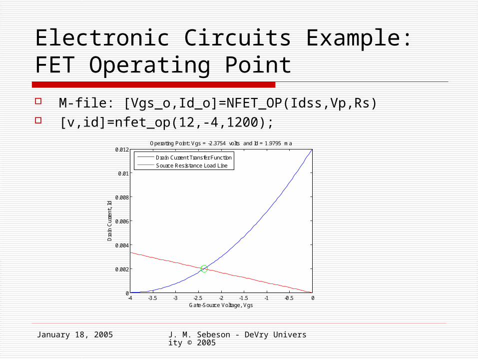
Electronic Circuits Example:FET Operating Point

Find the DC operating point of the following circuit:

2

1

P

GSDSSD

S

GSD

V

VII

R

VI


Electronic Circuits Example:FET Operating Point M-file: [Vgs_o,Id_o]=NFET_OP(Idss,Vp,Rs) [v,id]=nfet_op(12,-4,1200);

-4 -3.5 -3 -2.5 -2 -1.5 -1 -0.5 00

0.002

0.004

0.006

0.008

0.01

0.012

Gate-Source Voltage, Vgs

Dra

in C

urre

nt,

Id

Operating Point: Vgs = -2.3754 volts and Id = 1.9795 ma

Drain Current Transfer Function

Source Resistance Load Line


Physics Example:Graphical Solution of a Trajectory

Problem:A football kicker can give the ball an initial speed of 25 m/s. Within what two elevation angles must he kick the ball to score a field goal from a point 50 m in front of goalposts whose horizontal bar is 3.44 m above the ground?


Physics Example:Field Goal Problem

Solution: The general solution is the “trajectory equation.”

where y = height, x = distance from goal, v0 = take-off speed, θ0 = take-off angle. Given the take-off speed of 25 m/s, the problem requires the solutions for θ0 that result in a minimum height of y = 3.44 m at a distance of x = 50 m from the goal post. Although an analytical solution is possible, a graphical solution provides more physical insight.

)(cos2)tan(

022

0

2

0

v

gxxy


Physics Example:Field Goal Problem MATLAB code for a graphical solution:

>> v0=25;>> x=50;>> g=9.8;>> y=3.44;>> theta=5:.1:70;>> theta_r=theta*pi/180;>> z=y*ones(1,length(theta));>> zz=x*tan(theta_r)-g*x^2./(2*v0^2*(cos(theta_r)).^2);>> plot(theta,zz)>> holdCurrent plot held>> plot(theta,z)


Physics Example:MATLAB Results


Signal Processing Examples Fourier Synthesis and the Gibbs Phenomenon

“square_jms” m-file

Finite Impulse Response (FIR) Filter Design

Use of “fvtool”

Analog-to-Digital Converter Emulation “adc” m-file

Digital Transfer Function in the Z-domain “plotH” m-file

)(][ 00 nSINCnh

,...5,3,1

)2sin(2)(

1

n

n

ftnts

nsquare

Documents

Introduction to MATLAB MATLAB in Science, Engineering, and Mathematics Instruction John Sebeson DeVry University