Introduction to MATLAB - Isctecm.de.iscte.pt/IntrodMatlab_Students.pdf · Introduction Windows in MATLAB: 6 windows 1 Command window: to run the programs and to obtain the results

Introduction to MATLAB– Macroeconomics –

Vivaldo Mendes

Dep. Economics – Instituto Universitário de Lisboa

September 2017

(Vivaldo Mendes — ISCTE-IUL ) Macroeconomics September 2013 1 / 41

Summary

1 Introduction2 Functions, operations and vectors3 Matrices4 Real functions5 Importing data and representing time series6 Exercises


Introduction

I —Introduction


Introduction

What is Matlab?

1 The name tells all: MatrixLaboratory2 The package of numerical computation more powerful currentlyavailable

3 Also good for symbolic calculus (Symbolic Toolbox), but there arebetter ones here

4 A wonderful interface with Windows (or Mac): very friendly5 Very easy to program simple routines6 There are routines publicly available in the net ... for almosteverything ... but


Introduction

Basic information

1 Matlab —basic bibliographic references:

1 An introduction to Matlab, by David Griffi ths (see "Readings")2 A Practical Introduction to Matlab, by Mark S. Gockenbach (see"Readings")

3 Matlab & Simulink: A Tutorial, by Tom Nguyen(http://edu.levitas.net/Tutorials/Matlab/index.html)

4 Help of Matlab: very, very useful

2 In this course:

1 We do not wish students to be able to write down sophisticatedroutines

2 Just to use Matlab for simple things3 "m-files" are given to students4 Or "m-files" found in the net


Introduction

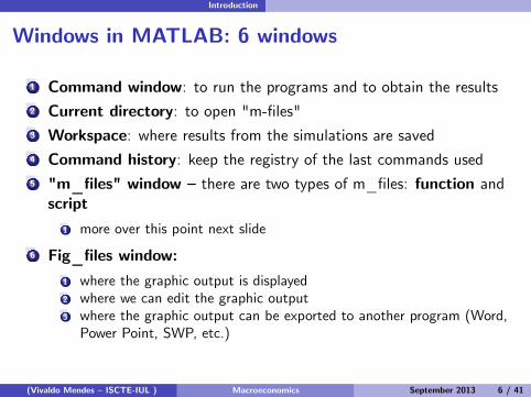
Windows in MATLAB: 6 windows

1 Command window: to run the programs and to obtain the results2 Current directory: to open "m-files"3 Workspace: where results from the simulations are saved4 Command history: keep the registry of the last commands used5 "m_files" window — there are two types of m_files: function andscript

1 more over this point next slide

6 Fig_files window:1 where the graphic output is displayed2 where we can edit the graphic output3 where the graphic output can be exported to another program (Word,Power Point, SWP, etc.)


Introduction

Functions vs Scripts

"m_files" window: we saw that there are 2 types:

1 function: this type of routine can only be run in the "commandwindow"

2 script: can be run directly from the run of the "m_file":

1 choose: debug + run

3 only when an ”m-file” is open, we know whether is script or afunction

1 function: it comes out with a text in blue indicatingfunction, forexample, the function: function f=par(x);f=x.^2

2 a script: no blue text indicating function


Introduction

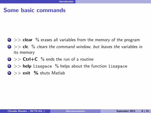
Some basic commands

1 >> clear % erases all variables from the memory of the program2 >> clc % clears the command window, but leaves the variables inits memory

3 >> Ctrl+C % ends the run of a routine4 >> help linspace % helps about the function linspace5 >> exit % shuts Matlab


Introduction

Numbers:types

1 Matlab recognizes various types of numbers2 Examples:


Introduction

Numbers: formatting

1 Matlab can present numbers in various different formats2 default format: assumed as "normal" by default3 Other formatting:

1 >> format short % number with 5 digits (1.1234)2 >> format long % number with 15 digits3 >> format short e % number in floating format with 5 digits4 >> format long e % number in floating format with 15 digits

4 Examples: next slide


Introduction

Numbers: formatting examples

Note that for numbers very small or very large, we may use the notation“e”, for example


Functions, operations and vectors

II —Functions, operations and vectors



Functions

1 Trigonometric functions:sin, cos, asin, acos, tan, atan, cot, acot

2 Other functions:1 exp (exponential)2 log (neperian logarithm)3 log10 (base 10)4 sqrt (square root)5 abs (absolute value)6 inf (infinit)7 erf (err function)



Operations

1 +, -, *, ^, / for numbers and matrices2 .+, .-, .*, .^, ./, for arrays (vectors of the same type)3 > larger, >= larger or equal, = = equal, ~= different4 >> nargin % Number of input arguments5 >> nargout % Number of output arguments6 >> varargin % Variable input argument list7 >> varargout % Variable output argument list



Vectors (arrays)1 >> v=1:3 , or >> v=[1,2,3] % defines the vector of integerelements 1,2,3

1 output: v = 1 2 32 >> u=[1:0.1:3] % defines the vector starting with 1, with anincrement of 0.1, and ending at 3

3 >> length(u) % to obtain the dimension of a vector:1 output: ans=21

4 Note 1: if we write at the end of command ";" (in example,u=[1:0.1:3];)

1 output does not show the values (or the variables), but keeps them inthe memory

5 Note 2: If nothing is added at the end of the command, keeps themin the memory and shows all the elements of the vector (21 overall)

1 output: Columns 1 through 7

1.0000 1.1000 1.2000 1.3000 1.4000 1.5000 1.6000Columns 8 through 141.7000 1.7000 .....(Vivaldo Mendes — ISCTE-IUL ) Macroeconomics September 2013 15 / 41


Vectors (arrays) —cont.

1 >> u=[1:4]; v=[3:6];2 >> u*v % incorrect operation

1 output: "??? Error using ==> mtimes

Inner matrix dimensions must agree."

1 >> u .*v % correct operation

1 output: ans = 3 8 15 24

2 >> v’ % transpose vector3 linspace: the vector x= [-1:0.1:1], (all the elements between −1and 1 with a step of 0.1) can be written

1 >> x = linspace(-1,1,21)


Matrices

III —Matrices


Matrices

Matrices

1 To represent a matrix A of type (3× 3) . For example

A =

1 0 −32 4 62 0 9

.

2 The elements in one line are separated by a common "," or space3 Lines are separated by ";"4 The command is:

>> A=[1,0,-3;2,4,6;2,0,9]

output: A =1 0 −32 4 62 0 9


Matrices

Matrices (cont.)1 >> A’ % transpose matrix AT of A2 >> A(:,i) % lists all elements of column i of matrix A3 >> A(i,:) % lists all elements of line i of matrix A4 >> A(i,j) % specifies the element in line i and column j5 >> inv(A) % calculates, if exists, the inverse matrix of A6 >> rank(A) % determines the characteristic of matrix A7 >> eye(n) % lists the identity matrix of order n8 >> ones(mxn) % matrix of type (m× n) , with all unit elements9 >> det(A) % calculates the determinant of A10 >> trace(A) % calculates the trace of matrix A11 >> eig(A) % calculates the eigenvalues of A12 >> poly(A) % characteristic polynomial of A13 >> norm(A) % norm of matrix A


Matrices

Matrices (cont.)

Operations with matrices

1 >> D = A + B; >> E = A * C; >> F = C * B

2 >> F1 = inv(sqrt(F)), >> G = B ./ A

3 >> sum(A) % sum of columns4 >> sum(sum(A)) % sum of all the elements5 >> A1 = sort(A) % separates the columns6 >> A2 = sort(A, 2) % separates the lines of a matrix

Example: determine the following (don´t type the ";")

1 Determine the inverse and the eigenvalues of A: inv(A), eig(A)2 Represent the second line and the first column of A:L2=A(2,:),C1=A(:,1)


Real functions

IV —Real functions


Real functions

Real functions with one real variable1 Representing graphically the function f (x) = x2 in the interval [−1, 1]

1 >>x = -1:0.1:1; f=x.^2; plot(x,f)

1 0.8 0.6 0.4 0.2 0 0.2 0.4 0.6 0.8 10

0.1

0.2

0.3

0.4

0.5

0.6

0.7

0.8

0.9

1


Real functions

Another way

1 Suppose we have the following m-file par.m saved in your partition2 This m-file represents the quadratic function above showed

function f=par(x)

f=x.^2;3 Using fplot in the Command Window

1 >> fplot(@par,[-1 1]) or fplot(’par’,[-1 1])

4 We get the graphic of our parable.5 Exercise: try it.


Real functions

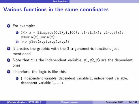
Various functions in the same coordinates

1 For example:

1 >> x = linspace(0,2*pi,100); y1=sin(x); y2=cos(x);y3=sin(x).*sin(x);

2 >> plot(x,y1,x,y2,x,y3)

2 It creates the graphic with the 3 trigonometric functions justmentioned

3 Note that x is the independent variable, y1, y2, y3 are the dependentones

4 Therefore, the logic is like this:

1 ( independent variable, dependent variable 1, independent variable,dependent variable 1„....)


Real functions

Various functions in the same coordinates

0 1 2 3 4 5 61

0.8

0.6

0.4

0.2

0

0.2

0.4

0.6

0.8

1


Real functions

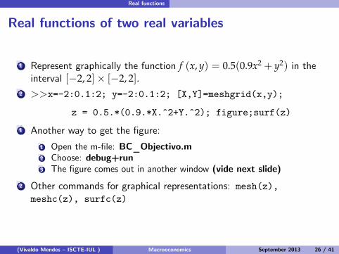
Real functions of two real variables

1 Represent graphically the function f (x, y) = 0.5(0.9x2 + y2) in theinterval [−2, 2]× [−2, 2].

2 >>x=-2:0.1:2; y=-2:0.1:2; [X,Y]=meshgrid(x,y);

z = 0.5.*(0.9.*X.^2+Y.^2); figure;surf(z)

1 Another way to get the figure:

1 Open the m-file: BC_Objectivo.m2 Choose: debug+run3 The figure comes out in another window (vide next slide)

2 Other commands for graphical representations: mesh(z),meshc(z), surfc(z)


Real functions

Real functions of two real variables (cont.)

2

1

0

1

2

2

1

0

1

20

0.5

1

1.5

2

2.5

3

3.5

4


Importing data and representing time series

V —Importing data and representing timeseries



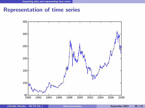
Representation of time series

1 Two forms of "importing" data into Matlab

1 Using the "Command Window"2 Using the submenu "Import data" from the main menu

2 An example using the "Command Window"

1 >> load temp.dat % importing the data from a temp file2 >> plot(temp) % does the figure with the data

3 Exemple —"Command Window"1 >> load portugal_aulas.txt2 >> figure; plot(portugal_aulas)3 >> days=linspace(1990,2008,4790);4 >> figure; plot(days,portugal_aulas)



Representation of time series

1990 1992 1994 1996 1998 2000 2002 2004 2006 200850

100

150

200

250

300

350



Representing two scales in the same coordinates

1 Sometimes it is very useful to represent in the same graphic twodifferent scales

1 >> plotyy(x1, y1, x2, y2)2 represents a function (or time series) y1 of variable x1 in the yy axisdefined on the left hand side of the graphic, and y2 of variable x2 inthe yy axis defined on the right hand side

2 Example :1 >> load USdata.txt2 >> GDP=USdata(:,3);3 >> INVENT=USdata(:,2);4 >> time=1947.0:0.25:2008.5;5 >> figure;6 >> plotyy(time,GDP,time,INVENT)



Representing two scales in the same coordinates(cont.)

1940 1950 1960 1970 1980 1990 2000 20100

5000

10000

15000

1940 1950 1960 1970 1980 1990 2000 2010100

0

100

200



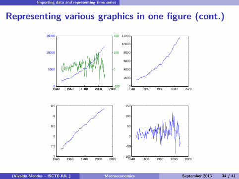
Representing various graphics in the same figure

Another very useful thing is to put various graphics in the same figure

A routine that puts 4 panels (graphics) inside 1 figure is:

>>load USdata.txt;GDP=USdata(:,3);INVENT=USdata(:,2);time=1947.0:0.25:2008.5;figuresubplot(221);plotyy(time,GDP,time,INVENT);subplot(222);plot(time,GDP);subplot(223);plot(time,log(GDP));subplot(224);plot(time,INVENT);

See result in the next slide



Representing various graphics in one figure (cont.)

1940 1960 1980 2000 20200

5000

10000

15000

1940 1960 1980 2000 2020100

0

100

200

1940 1960 1980 2000 20200

2000

4000

6000

8000

10000

12000

1940 1960 1980 2000 20207

7.5

8

8.5

9

9.5

1940 1960 1980 2000 2020100

50

0

50

100

150


Exercises

VI —Exercises


Exercises

The sustainability of public debt1 The evolution of nominal public debt (Dt) is given by

PtGt + it ·Dt−1 = PtTt +NewDebt︸︷︷︸Dt−Dt−1

2 P = general price level, T = real taxes, G = real governmentexpenditures, i = nominal interest rate on public debt

3 Designating Pt (Gt − Tt) = Ft as the primary deficit, we get

Dt −Dt−1 = Ft + it ·Dt−1

4 After a lengthy derivation, the public debt as a percentage of GDP(dt) is given by

dt = ft +(

1+ rt

1+ gt

)dt−1

5 where ft = primary deficit as a % of GDP, rt = real interest rate, gt =growth rate of real GDP


Exercises

The sustainability of public debt (cont.)1 Using (see PubliDebt_Simulations.m) Matlab and Excel, analyze thesustainability of Public Debt in two scenarios:

Scenario A : f = 0.02 r = 0.02 g = 0.03Scenario B : f = 0.01 r = 0.02 g = 0.03

2 Try to see what happens in different snaps of time:

1 25 years period2 50 years period3 150 years4 600 years

3 What happens if, between t = 600, t = 610, there is a shock toprimary deficits in both scenarios

1 f = 0.08 at t = [600, 610], and goes back again to normality aftert = 610

4 What do you conclude?


Exercises

Various cases of dynamic processes1 Linear difference equation (see Stable_Deterministic_Equilibrum.m)

yt = a0 + a1yt−1

2 The logistic function (see Logistic.m)

yt = a1 (1− yt−1) yt−1

3 A funny equation (strong nonlinearity: Self_fulfilling_Prophecies.m)

yt =a1y3

t−1 − a2y2t−1

24 An AR(1) process (see Stochastic_Equilibrum.m)

yt = a0 + a1yt−1 + εt , 0 < a1 6 1

5 An AR(1) process with a deterministic trend (Deterministic-trend.m)

yt = a0 + a1yt−1 + a2t+ εt , 0 < a1 6 1

a0, a1, a2 as parameters, εt ∼ iid(0, σ2), t is the long term trend of y(measured in logarithmic values)(Vivaldo Mendes — ISCTE-IUL ) Macroeconomics September 2013 38 / 41

Exercises

Bibliography


Exercises

Bibliography

David F. Griffi ths (2005). "An Introduction to Matlab (Version 2.3)",Department of Mathematics, The University Dundee. (36 pages, to bejust consulted, not to be studied)

Mark Gockenbach (1999). "A Practical Introduction to Matlab",Department of Mathematical Science, Michigan TechnologicalUniversity. (33 pages, to be just consulted, not to be studied)

William Palm III (2008). A Concise Introduction to MATLAB,McGraw-Hill, N.Y. As a book, you have to dive into several chaptersto cover most material presented in these slides. But the two firtschapters will be enough.


Exercises

Bibliography (cont.)

Cleve Moler (2004). Numerical Computing with MATLAB,MathWorks, the entire book available athttp://www.mathworks.com/moler/chapters.html. A goodintroduction to Matlab (in fact, more like an appetizer, rather thantrue introduction to the computing package) can be found in Chapter1 "Introduction to Matlab" (55 pages) of this book written by thefounder and CEO of Matlab.


Documents

Introduction to MATLAB - Isctecm.de.iscte.pt/IntrodMatlab_Students.pdf · Introduction Windows in MATLAB: 6 windows 1 Command window: to run the programs and to obtain the results