Introduction to Magnetic Resonance Imaging

Loan Vo, John Stastny

April 13, 2007

Contents

1 Objective 2

2 Introduction 22.1 Signal Generation . . . . . . . . . . . . . . . . . . . . . . . . . . . . . . . . . 2

2.1.1 The B0 field . . . . . . . . . . . . . . . . . . . . . . . . . . . . . . . . 22.1.2 The B1 or RF field . . . . . . . . . . . . . . . . . . . . . . . . . . . . 52.1.3 Free Induction Decays and Spin Echos . . . . . . . . . . . . . . . . . 6

2.2 Gradient Fields: Encoding Spatial Information . . . . . . . . . . . . . . . . . 72.2.1 Frequency Encoding . . . . . . . . . . . . . . . . . . . . . . . . . . . 72.2.2 Phase Encoding . . . . . . . . . . . . . . . . . . . . . . . . . . . . . . 8

2.3 The K-space Interpretation . . . . . . . . . . . . . . . . . . . . . . . . . . . . 82.3.1 Frequency Encoded Signals . . . . . . . . . . . . . . . . . . . . . . . 82.3.2 Phase Encoding Gradients . . . . . . . . . . . . . . . . . . . . . . . . 10

2.4 Basic Imaging Pulse Sequence . . . . . . . . . . . . . . . . . . . . . . . . . . 10

3 Fourier Reconstruction, Noise and Image Artifacts 123.1 Fourier Reconstruction . . . . . . . . . . . . . . . . . . . . . . . . . . . . . . 123.2 Noise . . . . . . . . . . . . . . . . . . . . . . . . . . . . . . . . . . . . . . . . 15

3.2.1 Noise in direct FFT Reconstruction . . . . . . . . . . . . . . . . . . . 153.2.2 Noise in zero-padded FFT Reconstruction . . . . . . . . . . . . . . . 16

3.3 Image Artifacts . . . . . . . . . . . . . . . . . . . . . . . . . . . . . . . . . . 163.3.1 Gibbs Ringing Artifact . . . . . . . . . . . . . . . . . . . . . . . . . . 163.3.2 Aliasing Artifact . . . . . . . . . . . . . . . . . . . . . . . . . . . . . 173.3.3 Motion Artifact . . . . . . . . . . . . . . . . . . . . . . . . . . . . . . 18

1

1 Objective

The objective of this laboratory is to familiarize the reader with the basic principle of mag-netic resonance imaging. This includes signal generation, data reconstruction, and sourcesof noise and artifacts in MRI. In addition, an emphasis will be placed on signal processingconcepts in MRI including the k-space, temporal and spatial under sampling, filtering, andFourier transform relationships.

2 Introduction

Magnetic resonance imaging (MRI) is an extremely versatile imaging modality, with a broadrange of clinical applications. Some of the most important applications of MRI are cardiacimaging, breast cancer imaging, brain imaging, fMRI, and spectroscopic imaging. MRI isbased on the principle of spin quantum mechanics. However, the well known Bloch equationsprovide a macroscopic description of MRI which is considerably easier to analyze. In thislab, we will begin by looking at the basic principles behind MRI signal generation.

2.1 Signal Generation

In MRI, we are concerned with three magnetic fields. These three magnetic fields are themain magnetic field (commonly called the B0 field), the B1 field (also called the RF pulse),and the gradient field (responsible for encoding spatial information). Next, we will look ateach of these fields, and their role in MRI.

2.1.1 The B0 field

In MRI the B0 field is a strong permanent magnetic field, typically 1 Tesla to 3 Tesla instrength. For some perspective, the earths magnetic field is around .5 gauss, where 1 gauss= 10−4 Tesla. The main magnetic field serves two roles in MRI. To understand these roles,we first look at the atomic basis for MRI.

We can think of individual atoms as magnetic dipoles, or spins. According to this de-scription, the magnetic moment of a spin is given by:

µ = γJ (1)

where J is the angular momentum, and γ is the gyromagnetic ration, which for hydrogenis given by

γ = 42.58MHz/T

The magnitude of the magnetic moment is given by;

|µ| = γh√

I(I + 1) (2)

where I is the spin quantum number, and h is planks constant over 2π. In the case of

spin 12

atoms, µ is allways√

32. It is important to note that µ is a vector quantity. In other

words,

2

Figure 1: Spin angular momentum and associated projection onto z-axis

J = xJx + yJy + zJz

The two possible orientations of µ with respect to a fixed axis (taken to be the z-axis) areshown in figure 1.

The bulk magnetization is given by the ensemble over the entire sample:

M =Ns∑

n=1

µn (3)

where Ns is the number of spins in the ensemble, and µn is given by (1).In general, an ensemble of spins will posses no bulk magnetization, since each spin has

random angular momentum, so that the summation over a large number of systems will givezero as shown in figure 3. However, if we place an ensemble of spins into a strong magneticfield oriented in the z-direction, the z-component of µn will cease to be random. Instead, thedistribution of µn,z will be given by the following expression;

N↑

N↓

= e∆EKTs (4)

where ∆E is the energy difference between the spin up and spin down states, Ts is thetemperature in kelvin, and K is Boltzman’s constant.

The energy corresponding to spin up and spin down states is given by +12γhB0 and

−12γhB0. The energy diagram is shown in figure 2. This effect is commonly known as

Zeeman splitting. In this figure, the frequency, rather than the energy is given. Note, thatthe energy difference, ∆E is given by:

∆E = γhB0 (5)

which corresponds to a frequency, 2πγB0 = ω0.By first order Taylor series approximation to (4), we may write:

N↑ − N↓ ≈ NsγhB0

2KTs

(6)

Equation (6) indicates there is a very small excess number of spin ups.Using (3) and (4), we find the total z bulk magnetization is given by:

3

Figure 2: Spin angular momentum and associated projection onto z-axis

Figure 3: Totally random spin angular momentum.

Mz0 =γ2h2B0Ns

4KTs

(7)

As an example, we consider the value for (7) for some typical values found in MRI.Take the following parameters:

Ts = 300K

B0 = 1Tesla

Then we get the following;

N↑ − N↓

Ns

=γhB0

2KTs

= 3 × 10−6 (8)

It is for this reason that MRI is known as a low sensitivity imaging modality. That is, avery small difference in the number of spin ups to spin downs produces all of the signal inMRI.

Remember that the total bulk x and y magnetization is still zero, since the x and ycomponents of the angular momentum are random, and hence sum to zero.

4

In addition to creating the Zeeman splitting effect, the B0 field causes the spins to precessabout the z-axis at a frequency known as the larmor frequency, given by:

ω0 = γB0 (9)

This frequency also corresponds to the energy difference between the spin up and spindown states. So in summary, the B0 field is responsible for the Zeeman splitting effect, andthe precession of spins.

Next, we look at the B1 field or RF field. From this point on, we conider the bulkmagnetization model, where the total z-magnetization in the presence of a magnetic field B0

is given by (7).

2.1.2 The B1 or RF field

The B1 field is an RF (radio frequency) pulse transmitted at a frequency corresponding tothe Larmor or resonance frequency, ω0. The manipulation of the bulk magnetization beginswith the application of the RF pulses. To understand how RF pulses work, we consideragain the energy diagram in figure (1). According to planks formula, a photon of frequencyω, has energy,

E = hω

Therefore, hitting a spin with a photon with frequency ω0 = γB0, will cause that spinto change states. In other words, when a spin with energy +1

2ω0 is hit with a photon of

frequency ω, it will jump to the spin down state, with an energy −12ω0. However, this is an

unstable state. This spin will eventually return to a spin up state, and in the process willemit a photon of frequency ω0.

This is the basic principle behind MRI, and the application of RF pulses. The RF pulsecauses spins to change to the opposite state. When these spins return to their original state,they emit photons (RF energy) at the same frequency, ω0.

We begin by considering the equilibrium magnetization, which we represent as a vectoras shown in figure 4. Initially, all magnetization is along the z-direction. The RF pulse canbe applied in any direction (x, y, -x, -y). The effect of the RF pulse on the magnetizationvector, M is to rotate the vector about the axis of RF application by an angle

α = γB1τ

where B1 is the strength of the RF pulse, and τ is the length of the RF pulse.For example, consider the effect of an αx pulse on the bulk magnetization vector,

M =

M0z

00

Immediately after the pulse, the magnetization components are:

Mx′(0+) = 0My′(0+) = M0

z sin αMz′(0+) = M0

z cos α

(10)

5

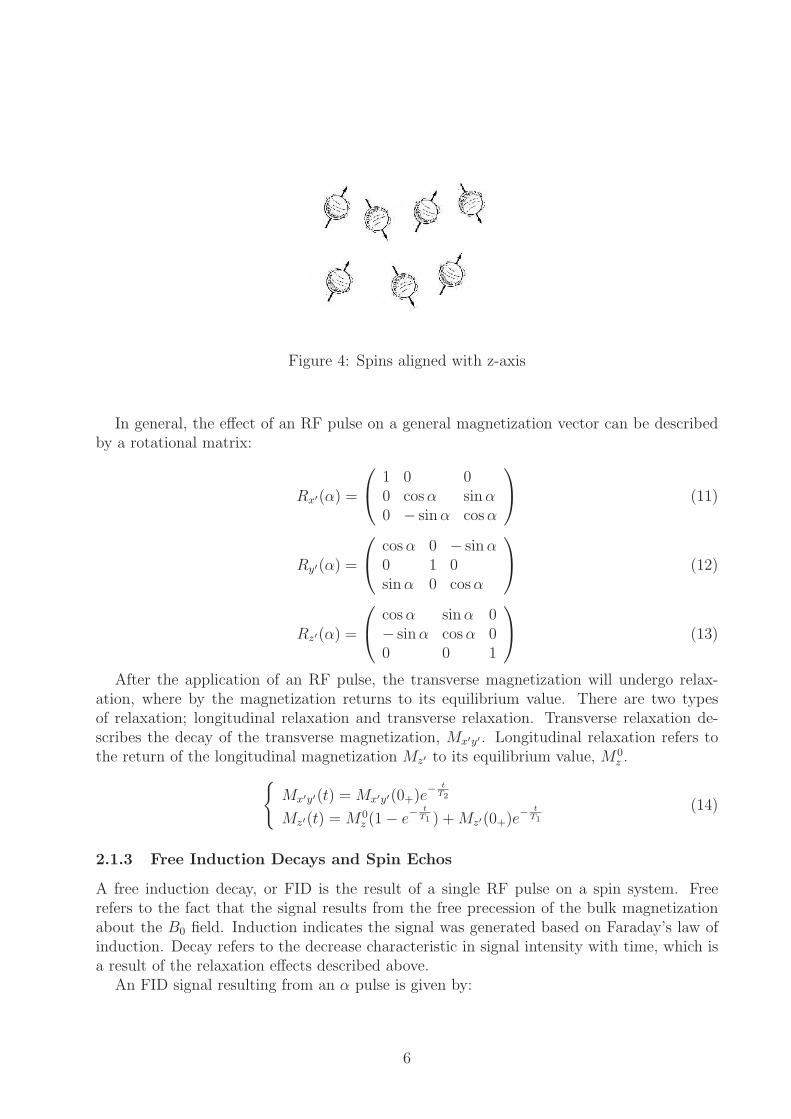
Figure 4: Spins aligned with z-axis

In general, the effect of an RF pulse on a general magnetization vector can be describedby a rotational matrix:

Rx′(α) =

1 0 00 cos α sin α0 − sin α cos α

(11)

Ry′(α) =

cos α 0 − sin α0 1 0sin α 0 cos α

(12)

Rz′(α) =

cos α sin α 0− sin α cos α 00 0 1

(13)

After the application of an RF pulse, the transverse magnetization will undergo relax-ation, where by the magnetization returns to its equilibrium value. There are two typesof relaxation; longitudinal relaxation and transverse relaxation. Transverse relaxation de-scribes the decay of the transverse magnetization, Mx′y′ . Longitudinal relaxation refers tothe return of the longitudinal magnetization Mz′ to its equilibrium value, M0

z .

{

Mx′y′(t) = Mx′y′(0+)e− t

T2

Mz′(t) = M0z (1 − e

− tT1 ) + Mz′(0+)e

− tT1

(14)

2.1.3 Free Induction Decays and Spin Echos

A free induction decay, or FID is the result of a single RF pulse on a spin system. Freerefers to the fact that the signal results from the free precession of the bulk magnetizationabout the B0 field. Induction indicates the signal was generated based on Faraday’s law ofinduction. Decay refers to the decrease characteristic in signal intensity with time, which isa result of the relaxation effects described above.

An FID signal resulting from an α pulse is given by:

6

S(t) = sin α

∫ ∞

−∞

ρ(ω)e− t

T2(ω) e−iωtdω (15)

where ρ(ω) is the spectral density function, which characterizes the spin system. Forexample, the FID from a system with a single spectral component is given by:

S(t) = M0z sin αe

− tT2 e−iω0t (16)

Spin echos are the result of the dephasing and rephasing of spins as a result of theapplication of two or more RF pulses. In the simplest case, we apply the pulse sequence:

90 − τ − 180

After the 90 degree pulse, the bulk magnetization vectors lie along the y’ axis. At thispoint, we consider two isochromats, at slightly different resonance frequencies, ωs and ωf ,representing a slow and fast isochromat respectively. During the delay, τ , these two isochro-mats dephrase. When the 180 degree pulse is applied, both of the bulk magnetization vectorsflip over the y’ axis. Finally, after another delay, τ , the two isochromats rephase, creating aspin echo. The pulse sequence and the associated spin echo signal are shown in ??

2.2 Gradient Fields: Encoding Spatial Information

After a signal has been activated by an RF pulse, spatial information can be encoded duringthe free precession period. There are two main ways to encode spatial information in MRI;frequency encoding and phase encoding.

2.2.1 Frequency Encoding

Frequency encoding makes the oscillation frequency of an activated MRI signal linearlydependent on spatial position. We first consider a one dimensional object, with an associatedspin density ρ(x). If we assume the object is exposed to a uniform B0 field, then under theinfluence of a linear gradient, G(x), the Larmor frequency at a position x is given by:

ω(x) = ω0 + γGxx (17)

Neglecting the transverse relaxation effect, the associated FID for a small area is:

dS(x, t) = ρ(x)dxe−iγ(B0+Gxx)tdx (18)

The received signal from the entire object under frequency encoding gradient is given by:

S(t) =

∫ ∞

−∞

ρ(x)e−iγ(B0+Gxx)tdx =

[∫ ∞

−∞

ρ(x)e−iγGxxtdx

]

e−iω0t (19)

After demodulation (removal of carrier signal e−iω0t), we get:

∫ ∞

−∞

ρ(x)e−iγGxxtdx (20)

7

In the more general case, where our phase encoding gradient is given by

Gfe = (Gx, Gy, Gz)

The signal expression in equation (20) is replaced by the expression:

S(t) =

∫

object

ρ(r)e−iγGfe·rtdr (21)

2.2.2 Phase Encoding

The principle behind phase encoding is very similar to that of frequency encoding. We beginonce again with a simple 1-D case. If we apply a gradient Gx for a short period of time Tpe,then our local signal is given by:

dS(x, t) =

{

ρ(x)e−iγ(B0+Gxx)t 0 ≤ t ≤ Tpe

ρ(x)e−iγGxxTpee−iω0 Tpe ≤ t(22)

After the phase encoding gradient is shut off, all of the spin systems will again precess atthe same frequency ω0. However, each will have a different phase, given by:

φ(x) = −γGxxTpe (23)

2.3 The K-space Interpretation

In this section, we draw the connection between spatial encoding (phase encoding and fre-quency encoding), and the Fourier Transform. This connection provides us the means toanalyze complex pulse sequences using the k-space notation.

2.3.1 Frequency Encoded Signals

We first consider the frequency encoded signal, given by (20). Making a simple variablesubstitution, we obtain the following Fourier transform relationship.

S(kx) =

∫ ∞

−∞

ρ(x)e−i2πkxxdx (24)

where kx is given by;

kx =

{

2πγGxt FID signals2πγGx(t − TE) echo signals

(25)

This expression can be easily extended to the case when we have multiple frequencyencoding gradient:

k =

{

2πγGfet FID signals2πγGfe(t − TE) echo signals

(26)

The corresponding k-space signal according to is,

8

S(k) =

∫

object

ρ(r)e−i2πk·rdr (27)

It is important to note that although the k-space signal is a multidimensional Fouriertransform, the signal S(k), is available only at a limited set of discrete points in k-space.These k-space points define the sampling trajectory of k-space.

For example, in the two dimensional case where we have an FID which is frequencyencoded, we get the following k-space sampling trajectory.

{

kx = 2πγGxtky = 2πγGyt

(28)

or

{

kx = k cos φky = k sin φ

(29)

wherek = 2πγGfet = 2πγt

√

G2x + G2

y (30)

and

φ = tan−1

(

Gy

Gx

)

(31)

Equation 29 describes a straight line through the origin of k-space as shown in figure ??.These same conclusions can be easily extended to 3 dimensions. In this case, we have:

kx = k sin θ cos φky = k sin θ sin φkz = k cos θ

(32)

wherek = 2πγGfet = 2πγt

√

G2x + G2

y + G2z (33)

θ = tan−1

(

√

G2x + G2

y

Gz

)

(34)

and

φ = tan−1

(

Gy

Gx

)

(35)

In the most general case, where Gfe is a function of time, the mapping between Gfe(t)and k is given by;

k(t) = 2πγ

∫ t

0

Gfe(τ)dτ (36)

One very important point to address is the effect of a 180 degree RF pulse on the k-spacetrajectory. The following example will address this issue.

9

Recall that the effect of a 180 degree pulse on the transverse magnetization is given by:

Mx′y′

πϕ−→ M∗x′y′e−i2ϕ (37)

which can also be expressed as:

Mx′y′ = ρ(r)drei2πk·r (38)

then the postpulse transverse magnetization is given by;

Mx′y′ = ρ(r)drei(2πk·r−2ϕ) (39)

It is clear from equations (38) and (39) that

kπϕ−→ −k (40)

2.3.2 Phase Encoding Gradients

Next, we consider the effect of the phase encoding gradient in terms of the Fourier Transform.We can express the phase encoded signal in 22 as

S(k) =

∫

object

ρ(r)e−i2πk·rdr (41)

if we drop the carrier signal, e−iω0t, and make the variable substitution:

k =γ

2πGpeTpe (42)

It is important to note that, unlike in the case of the frequency encode gradient, we arenot taking samples of k-space during a phase encode. Rather, we simply travel in k spaceaccording to equation (42). In the general case, where we do not have a rectangular phaseencode gradient, k is given by:

S(k) =γ

2π

∫ Tpe

0

Gpe(τ)dτ (43)

2.4 Basic Imaging Pulse Sequence

In this section, we look at the most basic imaging sequence, and consider the associatedk-space sampling trajectory. The pulse sequence to be considered is shown in figure 5.

To understand how the k-space is sampled in this scheme, we consider the nth excitation.

{

kx = γ2π

Gx(t − t0) t0 < t < Tacq/2 + t0ky = γ

2πn∆Gy(t − t0)

(44)

Which represents a radial line from the origin to point A, defined by:

kA = (γ

2πGxTpe,

γ

2πn∆GyTpe) (45)

The effect of the 180 degree pulse is to flip the k space point to B:

10

RF

TE/2

90

TE/2

180Acquire

Gx

Tpe Tacq

Gy

Tpe

Figure 5: Basic Imaging pulse sequence.

Figure 6: The k-space trajectory for 1 repetition of the basic imaging pulse sequence

kB = −kA (46)

During the data acquisition interval, the k-space sampling points are given by:

{

kx = γGx(t − TE) |t − TE| < Tacq/2ky = γn∆GyTpe

(47)

The corresponding k-space trajectory of this one excitation is shown in figure 6This represents a single horizontal line in k-space. In this imaging scheme, we repeat

this pulse sequence N times, changing the phase encode gradient Gy each time. In this way,we collect N lines in k-space. With this k-space data, we can recover the underlying imagefunction, ρ(x, y). It is important to note here that the time required for the entire imagingexperiment is roughly proportional to the number of phase encodes. That is, application ofthe pulse sequence shown in 5 takes a time TR, then the total time for this experiment is:

11

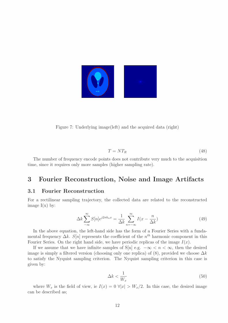
Figure 7: Underlying image(left) and the acquired data (right)

T = NTR (48)

The number of frequency encode points does not contribute very much to the acquisitiontime, since it requires only more samples (higher sampling rate).

3 Fourier Reconstruction, Noise and Image Artifacts

3.1 Fourier Reconstruction

For a rectilinear sampling trajectory, the collected data are related to the reconstructedimage I(x) by:

∆k

∞∑

−∞

S[n]ej2πknx =1

∆k

∞∑

n=−∞

I(x − n

∆k) (49)

In the above equation, the left-hand side has the form of a Fourier Series with a funda-mental frequency ∆k. S[n] represents the coefficient of the nth harmonic component in thisFourier Series. On the right hand side, we have periodic replicas of the image I(x).

If we assume that we have infinite samples of S[n] e.g. −∞ < n < ∞, then the desiredimage is simply a filtered version (choosing only one replica) of (8), provided we choose ∆kto satisfy the Nyquist sampling criterion. The Nyquist sampling criterion in this case isgiven by:

∆k <1

Wx

(50)

where Wx is the field of view, ie I(x) = 0 ∀|x| > Wx/2. In this case, the desired imagecan be described as;

12

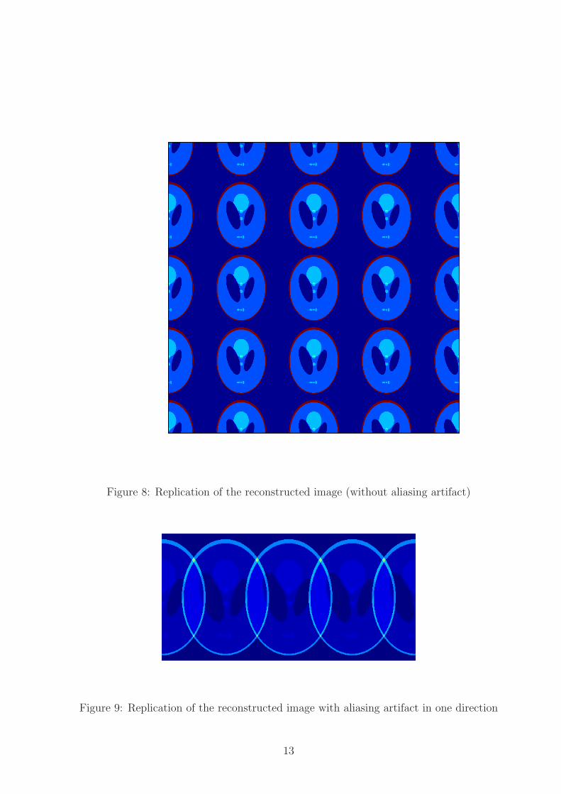
Figure 8: Replication of the reconstructed image (without aliasing artifact)

Figure 9: Replication of the reconstructed image with aliasing artifact in one direction

13

I(x) = ∆k

∞∑

−∞

S[n]ej2πknx |x| <1

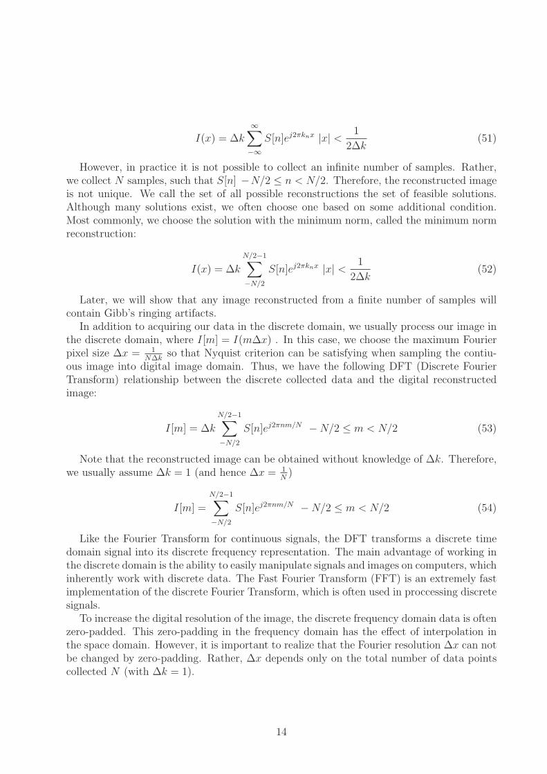
2∆k(51)

However, in practice it is not possible to collect an infinite number of samples. Rather,we collect N samples, such that S[n] −N/2 ≤ n < N/2. Therefore, the reconstructed imageis not unique. We call the set of all possible reconstructions the set of feasible solutions.Although many solutions exist, we often choose one based on some additional condition.Most commonly, we choose the solution with the minimum norm, called the minimum normreconstruction:

I(x) = ∆k

N/2−1∑

−N/2

S[n]ej2πknx |x| <1

2∆k(52)

Later, we will show that any image reconstructed from a finite number of samples willcontain Gibb’s ringing artifacts.

In addition to acquiring our data in the discrete domain, we usually process our image inthe discrete domain, where I[m] = I(m∆x) . In this case, we choose the maximum Fourierpixel size ∆x = 1

N∆kso that Nyquist criterion can be satisfying when sampling the contiu-

ous image into digital image domain. Thus, we have the following DFT (Discrete FourierTransform) relationship between the discrete collected data and the digital reconstructedimage:

I[m] = ∆k

N/2−1∑

−N/2

S[n]ej2πnm/N − N/2 ≤ m < N/2 (53)

Note that the reconstructed image can be obtained without knowledge of ∆k. Therefore,we usually assume ∆k = 1 (and hence ∆x = 1

N)

I[m] =

N/2−1∑

−N/2

S[n]ej2πnm/N − N/2 ≤ m < N/2 (54)

Like the Fourier Transform for continuous signals, the DFT transforms a discrete timedomain signal into its discrete frequency representation. The main advantage of working inthe discrete domain is the ability to easily manipulate signals and images on computers, whichinherently work with discrete data. The Fast Fourier Transform (FFT) is an extremely fastimplementation of the discrete Fourier Transform, which is often used in proccessing discretesignals.

To increase the digital resolution of the image, the discrete frequency domain data is oftenzero-padded. This zero-padding in the frequency domain has the effect of interpolation inthe space domain. However, it is important to realize that the Fourier resolution ∆x can notbe changed by zero-padding. Rather, ∆x depends only on the total number of data pointscollected N (with ∆k = 1).

14

3.2 Noise

In MRI, the acquired k-space data are contaminated by noise. To analyze the noise char-icteristics of the acquired signal, and how this noise effects the reconstructed image, weconsider the following. We assume that the noise at all k-space locations, is independent andidentically distributed (iid) gaussian, with zero mean and variance σ2

d. We denote this noiseas ξd[m]. Furthermore, we denote the noise corrupted k-space signal and noise corruptedimage as S, I , respectively. The clean k-space signal and clean image are represented as Sand I, respectively.

We assume the following additive model for the noise corrupted k-space signal S(k):

S(k) = S(k) + ξd(k) (55)

Taking the 2-D Fourier transform of this noise corrupted data results in the noisy image;

I(x) = I(x) + ξI(x) (56)

3.2.1 Noise in direct FFT Reconstruction

Next, we consider the case of applying a discrete Fourier Transform to the discrete data inthe presence of noise.

In this case, the image noise is related to the k-space noise by:

ξ[m] =1

N

N/2−1∑

−N/2

ξd[n]ej2πnm/N − N/2 ≤ m < N/2 (57)

Using this expression, we find the first order statistics of the image noise:

E{ξI [m]} = 0 (58)

σ2I =

1

Nσ2

d (59)

E{ξI [m]ξ∗I [n]} = 0 m 6= n (60)

Using (60), it is easy to prove that the signal to noise ratio (SNR) at each pixel locationis:

SNR|pixel =Iavg

σI

(61)

=

1N

∑N/2−1−N/2 I[m]I∗[m]

σI

(62)

=

√

∑N/2−1n=−N/2 |S[n]|2√

NσI

(63)

It is clear from this expression that the SNR decreases as the total number of encodingsincreases. This trade off between spatail resolution, (primarily in the frequency encode

15

direction), and SNR is important to keep in mind. Although increasing the number offrequency encodings may not greatly increase the acquisition time, it will degrade the SNR.

In the image domain, the noise still has uncorrelated variance from pixel to pixel. There-fore, SNR can be improved by taking the average value of several adjacent pixels in an image.Once again, we trade off spatial resolution for SNR. We denote I1[m] as the noise-corruptedFFT image and I2[m] as:

I2[m] =1

P

P−1∑

p=0

I1(m + p) (64)

where P is the number of adjacent pixels averaged. Then it is clear that the SNR of I2[m]is improved by a factor of

√P as compare with SNR of I1[m]

3.2.2 Noise in zero-padded FFT Reconstruction

In this section, we explore the effect of zero-padding on the noise charicteristics. We considerzero-padding our k-space signal from N points to M point, to produce an image of length M.In this case, our new image noise is given by;

ξ[m] =1

N

N/2−1∑

−N/2

ξd[n]ej2πnm/N − M/2 ≤ m < M/2 (65)

Therefore, we also have:

E{ξI [m]} = 0 (66)

σ2I =

1

Nσ2

d (67)

E{ξI [m]xi∗I [n]} = 1/N2σ2d

sin[π(m − n)N/M ]

sin[π(m − n)/M ]e−iπ(m−n)/N m 6= n (68)

Zero-padding does not change the image noise mean or variance. Consequently, the SNRin the zero-padded image is identical to that of the non zero-padded image. At this point, theobservent reader may ask why we do not simply average the extra adjacent pixels to increase

SNR by a factor of√

1P. In this case, the noise at adjacent pixels is not independent, and

so averaging adjacent pixels will not improve SNR.

3.3 Image Artifacts

3.3.1 Gibbs Ringing Artifact

In this section, we explore the phenomena of Gibbs ringing in MRI. In MRI, we musttruncate our k-space data to collect a finite number of k-space samples. As a result, the highfrequency components of the data are discarded. The resulting image is actually the resultof a convolution between the ideal image and the point spread function:

16

h(x) = ∆k

N/2−1∑

n=−N/2

e−iπ∆kx (69)

= ∆ksin(πN∆kx)

sin(π∆kx)e−iπ∆kx (70)

(71)

This artifact is commonly referred to as the Gibbs Ringing Artifact. The Gibbs phe-nomenon causes spurious ringing around sharp edges (Also note that, the maximum under-shoot or overshoot of the spurious ringing is about 9% of the intensity discontinuity and itdoes NOT depend on the number of data points used in the reconstruction).

In a 2D reconstructed image, Gibbs ringing can appear in both frequency and phaseencoding directions. However, the Gibbs ringing artifact is more pronounced in the phaseencoding direction. This is because the number of phase encodes we can collect is heavilyconstrained by the desired imaging time.

Although the Gibbs ringing artifact can be reduced by acquiring more high frequencyk-space points, in practice it is not always possible due to time requirements. However, aswe have discussed, it is releatively easy to increase the number of frequency encode points,and therefore reduce the Gibbs ringing artifact in this direction. Another commonly usedapproach in reducing the Gibbs ringing artifact is known as windowing. In windowing, awindow function is used to suppress the oscillations of the original point spread function:

I(x) = ∆k

N/2−1∑

−N/2

S(n∆k)wnej2πknx (72)

where wn is the window function, which clearly acts as a filter. The reduction in Gibbsringing artifact by a window function can be understood by looking at the point spread func-tion with windowing, h(x) = ∆k

∑N/2−1n=−N/2 wne

−iπ∆kx. A proper choice of window functionscan lead to a smoother behavior in the overall point spread function.

Although applying a window function can reduce the Gibbs ringing artifact, a trade-offdoes exist. This trade off is a reduction in spatial resolution (blurring). Spatial resolution isreduced due to an increase in the effective width of the point spread function after windowing.

In addition to windowing, several other techniques exist for reducing Gibbs ringing. Forexample, the Generalized Series reconstruction (known as RIGR or TRIGR) algorithm takesadvantage of known information regarding the data to reconstruct high spatial resolutionimages from a limited number of k-space points.

3.3.2 Aliasing Artifact

As mention in (49), the Fourier series reconstruction of the collected data S(k) representsmany replicas or the desired image;

I(x) =∞∑

n=−∞

I(x − n

∆k) (73)

17

Figure 10: Gibbs ringing artifact. Top-left image is the original phantom image. Top-right,bottom-left and bottom-right images have Gibbs ringing in phase-direction only, frequency-direction only and both of the frequency and phase direction.

Violating the Nyquist condition (under-sampling in k-space) will cause these replicas towrap-around and overlap each other. This phenomena is commonly called aliasing. Ingeneral it is difficult to fix aliasing in post-processing. Therefore, it is important to satisfythe Nyquist criterion, or to use an anti-aliasing filter to limit the signal bandwidth.

3.3.3 Motion Artifact

In many practical applications, the object being imaged is not stationary. This leads to a socalled motion artifacts. Depending on the acquisition scheme as well as the type of motion,artifacts appear in the reconstructed image in a variety of forms. Blurring and ghosting arethe two most common motion artifacts. In this section, we are not going to discuss abouttechniques to overcome motion effects; however brief description how motion artifacts areintroduced and appear in reconstructed images will be provided.

Since there are big differences between phase and frequency encodings, object motioneffects are not the same in these two directions. The main difference is that motion effectsalong the phase direction seem to introduce more serious artifacts in reconstructed imagesbecause the time between two phase encodings is much larger than the time between twofrequency encodings. However, since there is no phase accumulation between phase encod-ings, analyzing motion effect along the phase encoding is easier. Let now begin to investigatemotion effect along the frequency encoding direction.

Motion Effects along the frequency-encoding direction (readout direction)

18

Figure 11: Aliasing artifact. Top-left image has no aliasing artifact. Top-right, bottom-leftand bottom-right image have aliasing artifact with the reduced encoding factor equal to 2,4 and 8

Let assume that object motion has constant velocity ~v = vx~i + vy

~j. Also denote I(x,y,0)as the object function at time 0 and I(x,y,t) as the object at time instant t. We have:

I(x, y, t) = I(x(t), y(t), 0) (74)

where

x(t) = x + vxt

y(t) = y + vyt (75)

As we know that readout gradient generates a phase component:

φ = γ

∫ t

0

~G(τ) · ~r(τ)dτ (76)

Assume that ~G(t) = Gx(t)~i, then φ in equation (eqn:phiReadOut) can be expressed as :

φ = γ

∫ t

0

Gx(τ)(x + vxτ)dτ

= γx

∫ t

0

Gx(τ) + γvx

∫ t

0

τGx(τ)dτ (77)

The first term in equation (77) is useful spatial encoding component. On the other hand,the second term leads to undesirable phase shifts - which are introduced by the motionvelocity. Denote this motion-dependent phase shift as ∆φ, we have:

19

∆φ = γvx

∫ t

0

τGx(τ)dτ (78)

If the readout gradient ~G(t) has the following from:

~G =

{

−Gx 0 ≤ t ≤ TE

2

GxTE

2≤ t ≤ 3TE

2

then the corresponding undesirable phase shift during the corresponding period is asfollowing:

∆φ =

{

−γvx

∫ t

0τGxdτ = −1

2γvxGxt

2 0 ≤ t ≤ TE/2

−12γvxGx(

TE

2)2 + γvx

∫ t

TE/2τGxdτ = 1

2γvxGx(t

2 − 2TE

2) TE

2≤ t ≤ 3TE

2

From equation 3.3.3, it is obvious that the peak of the echo signal is no longer at t = Tacq.In short, motion effects along the readout direction can be expressed in the following pointspread function h(x) (see [1] for detailed derivations).

h(x) ≈ (1 − i)√

π√γGxvx

e−iγGxvx(TE2

)2eiγ((x−xs)2)

vx (79)

where xs = vxTE - the distance object has moved in duration TE.

In equation (79), the term e−iγGxvx(TE2

)2 imposes phase shifts onto reconstructed images.If vx is constants, this phase shift component can be ignore. But if vx changes within avoxel, signal intensity will vary within the voxel. In general, along the direction in with vx

varies, dephasing will occur and create artifact in that direction (this artifact is analogousto the artifact introduced by motion in the phase encoding direction). The second term inthe equation (79) leads to image blurring in reconstruction.

Motion Effects along the phase-encoding directionLet assume that a constant phase encoding gradient Gn is used along the x-direction,

starting at tn and ending at tn + τ for the nth phase encoding, we have:

φn =∫ tn+τ

tnGn(x + vxt)dt

= γxτ + γGnvxτ(tn + τ/2)= 2πknx + 2πknvx(tn + τ/2)

where kn = γ/2πGnτHence, the undesirable phase shift along the phase encoding direction is

∆φ = 2πknvx(tn + τ/2) = 2πknvxtn + 2πknvxτ/2 (80)

Since linear phase shift only introduces spatial displacement in the reconstruction, wewon’t consider more the effect of the linear phase term 2πknvxτ/2. Let rewrite ∆φ asfollowing:

∆φ = 2πknvxtn (81)

Denote I(x, 0) (or I0) and I(x, tn) are snapshot images at time 0 and time tn. DenoteS0(kn) and S(kn) as the collected signal at the nth phase encodings of the object at time

20

0 (I0) and time tn (I(x, tn)) correspondingly. Then, the phase shift component in equation(81) imposes the following relationship between S(kn) and S0(kn):

S(kn) =∫∞

−∞I(x, tn)e−i2πknxdx

= e−i2πknvxtn∫∞

−∞I0e

−i2πknxdx

= e−i2πknvxtnS0(kn)

More general, we have:

S(k, t) =

∫ ∞

−∞

I(x, t)e−i2πkxdx (82)

The above equation can be interpreted as simply as the fact that there is a Fouriertransform relationship between object and collected data at any instantaneous time t. Italso means that if we want to reconstructed image having no motion artifact we need toacquire the whole k-space data instantaneous.

References

[1] Z.-P. Liang and P. C. Lauterbur, Principles of Magnetic Resonance Imaging: A Signal

Processing Perspective. SPIE, 2000.

21