Embed Size (px)
Citation preview

Department of Mechanical Engineering Prepared By: Mr. SUNIL G. JANIYANI Darshan Institute of Engineering & Technology, Rajkot Page 1.1
1 INTRODUCTION TO MACHINE DESIGN
Course Contents
1.1 Introduction to Machine
Design
1.2 Standardization
1.3 Preferred Numbers
Examples
1.4 Aesthetic Considerations
1.5 Ergonomic Considerations
1.6 Manufacturing
considerations in Design
1.7 Material Selection in
Machine Design
1.8 Mechanical Properties of
Metals
1.9 Effect of Impurities on Steel
1.10 Effects of Alloying Elements
on Steel
1.11 Heat Treatment of Steels

1. INTRODUCTION TO MACHINE DESIGN Design of Machine Elements (2151907)
Prepared By: Mr. SUNIL G. JANIYANI Department of Mechanical Engineering Page 1.2 Darshan Institute of Engineering & Technology, Rajkot
1.1 Introduction to Machine Design
The subject Machine Design is the creation of new and better machines and
improving the existing ones.
A new or better machine is one which is more economical in the overall cost of
production and operation.
The process of design is a long and time consuming one. From the study of existing
ideas, a new idea has to be conceived.
The idea is then studied keeping in mind its commercial success and given shape and
form in the form of drawings.
In designing a machine component, there is no rigid rule. The problem may be
attempted in several ways.
However, the general procedure to solve a design problem is discussed below.
1.1.1 General Procedure in Machine Design
Fig 1.1 General Procedure in Machine Design
1. Recognition of need:
First of all, make a complete statement of the problem, indicating the
need, aim or purpose for which the machine is to be designed.
2. Synthesis (Mechanisms):
Select the possible mechanism or group of mechanisms which will give
the desired motion.
3. Analysis of forces:
Find the forces acting on each member of the machine and the energy
transmitted by each member.

Design of Machine Elements (2151907) 1. INTRODUCTION TO MACHINE DESIGN
Department of Mechanical Engineering Prepared By: Mr. SUNIL G. JANIYANI Darshan Institute of Engineering & Technology, Rajkot Page 1.3
4. Material selection:
Select the material best suited for each member of the machine.
5. Design of elements (Size and Stresses):
Find the size of each member of the machine by considering the force
acting on the member and the permissible stresses for the material used.
It should be kept in mind that each member should not deflect or deform
than the permissible limit.
6. Modification:
Modify the size of the member to agree with the past experience and
judgment to facilitate manufacture.
The modification may also be necessary by consideration of
manufacturing to reduce overall cost.
7. Detailed drawing:
Draw the detailed drawing of each component and the assembly of the
machine with complete specification for the manufacturing processes
suggested.
8. Production:
The component, as per the drawing, is manufactured in the workshop.
1.2 Standardization
Standardization is defined as obligatory (or compulsory) norms, to which various
characteristics of a product should comply (or agree) with standards.
The characteristics include materials, dimensions and shape of the component,
method of testing and method of marking, packing and storing of the product.
There are two words – “standard and code” which are often used in standards .
A standard is defined as a set of specifications for parts, materials or processes. The
objective of, a standard is to reduce the variety and limit the number of items to a
reasonable level.
On the other hand, a code is defined as a set of specifications for the analysis, design,
manufacture, testing and erection of the product. The purpose of a code is to
achieve a specified level of safety.
There are three types of standards used in design office. They are as follows:
(i) Company Standards: They are used in a particular company or a group of
sister concerns.
(ii) National standards:
India - BIS (Bureau of Indian Standards),
Germany - DIN (Deutsches Institut für Normung),
USA - AISI (American Iron and Steel Institute) or SAE (Society of Automotive
Engineers),
UK - BS (British Standards)

1. INTRODUCTION TO MACHINE DESIGN Design of Machine Elements (2151907)
Prepared By: Mr. SUNIL G. JANIYANI Department of Mechanical Engineering Page 1.4 Darshan Institute of Engineering & Technology, Rajkot
(iii) International standards: These are prepared by the International Standards
Organization (ISO).
The following standards are used in mechanical engineering design:
(i) Standards for Materials, their chemical compositions, Mechanical properties
and Heat Treatment:
For example, Indian standard IS 210 specifies seven grades of grey cast iron
designated as FG 150, FG 200, FG 220, FG 260, FG 300, FG 350 and FG 400.
The number indicates ultimate tensile strength in N/mm2.
(ii) Standards for Shapes and dimensions of commonly used Machine Elements:
The machine elements include bolts, screws and nuts, rivets, belts and
chains, ball and roller bearings, wire ropes, keys and splines, etc.
For example, IS 2494 (Part 1) specifies dimensions and shape of the cross-
section of endless V-belts for power transmission.
The dimensions of the trapezoidal cross-section of the belt, viz. width, height
and included angle are specified in this standard.
(iii) Standards for Fits, Tolerances and Surface Finish of Component:
For example, selection of the type of fit for different applications is illustrated
in IS 2709 on 'Guide for selection of fits'.
The tolerances or upper and lower limits for various sizes of holes and shafts
are specified in IS 919 on 'Recommendations for limits and fits for
engineering'.
IS 10719 explains method for indicating surface texture on technical
drawings.
(iv) Standards for Testing of Products:
These standards, sometimes called 'codes', give procedures to test the
products such as pressure vessel, boiler, crane and wire rope, where safety of
the operator is an important consideration.
For example, IS 807 is a code of practice for design, manufacture, erection
and testing of cranes and hoists.
The method of testing of pressure vessels is explained in IS 2825 on 'Code for
unfired pressure vessels’.
(v) Standards for Engineering of Components:
For example, there is a special publication SP46 prepared by Bureau of Indian
Standards on 'Engineering Drawing Practice for Schools and Colleges' which
covers all standards related to engineering drawing.
1.2.1 Benefits of Standardization
Reductions in types and dimensions of identical components (inventory
control).
Reduction in manufacturing facilities.
Easy to replace (Interchangeability).

Design of Machine Elements (2151907) 1. INTRODUCTION TO MACHINE DESIGN
Department of Mechanical Engineering Prepared By: Mr. SUNIL G. JANIYANI Darshan Institute of Engineering & Technology, Rajkot Page 1.5
No need to design or test the elements.
Improves quality and reliability.
Improves reputation of the company which manufactures standard
components.
Sometimes it ensures the safety.
It results in overall cost reduction.
1.3 Preferred Numbers
With the acceptance of standardization, there is a need to keep the standard sizes or
dimensions of any component or product in discrete steps.
The sizes should be spread over the wide range, at the same time these should be
spaced properly.
For example, if shaft diameters are to be standardized between 10 mm and 25 mm,
then sizes should be like : 10 mm, 12.5 mm, 16 mm, 20 mm, 25 mm and not like : 10
mm, 11 mm, 13 mm, 18 mm, 25 mm.
This led to the use of geometric series known as series of preferred numbers or
preferred series.
Preferred series are series of numbers obtained by geometric progression and
rounded off.
There are five basic series with step ratios of:
√
√
√
√
√
These ratios are approximately equal to 1.58, 1.26, 1.12, 1.06 and 1.03.
The five basic series of preferred numbers (known as preferred series) are
designated as: R5, R10, R20, R40, and R80.
These series were first introduced by the French engineer Renard hence denoted by
the symbol R.
Each series is established by taking the first number one and multiplying it by a
constant (or step or G.P.) ratio to get the second number.
The second number is then multiplied by a step ratio to get the third number. The
procedure is continued until the complete series is built up.
The examples of preferred number series are: standard shaft diameters, power
rating of coupling, centre distances of standard gear boxes, etc.
The other series called derived series may be obtained.
Series R 10/3 (1, ... ,10) indicates a derived series comprising of every third term of
the R10 series and having the lower limit as 1 and higher limit as 10.
The advantages of preferred series are as follows :
(i) The difference in two successive terms has a fixed percentage.
(ii) It provides small steps for small quantities and large steps for large
quantities.
(iii) The product range is covered with minimum number of sizes without
restricting the choice of the customers.

1. INTRODUCTION TO MACHINE DESIGN Design of Machine Elements (2151907)
Prepared By: Mr. SUNIL G. JANIYANI Department of Mechanical Engineering Page 1.6 Darshan Institute of Engineering & Technology, Rajkot
Following table shows basic series of preferred numbers according to IS: 1076 (Part I)
– 1985 (Reaffirmed 1990).
Table 1.1 Basic series of preferred numbers
R5 R10 R20 R40
1.00 1.00 1.00 1.00
1.06
1.12 1.12
1.18
1.25 1.25 1.25
1.32
1.40 1.40
1.50
1.60 1.60 1.60 1.60
1.70
1.80 1.80
1.90
2.00 2.00 2.00
2.12
2.24 2.24
2.36
2.50 2.50 2.50 2.50
2.65
2.80 2.80
3.00
3.15 3.15 3.15
3.35
3.55 3.55
3.75
4.00 4.00 4.00 4.00
4.25
4.50 4.50
4.75
5.00 5.00 5.00
5.30
5.60 5.60
6.00
6.30 6.30 6.30 6.30
6.70
7.10 7.10
7.50
8.00 8.00 8.00
8.50
9.00 9.00
9.50
10.00 10.00 10.00 10.00

Design of Machine Elements (2151907) 1. INTRODUCTION TO MACHINE DESIGN
Department of Mechanical Engineering Prepared By: Mr. SUNIL G. JANIYANI Darshan Institute of Engineering & Technology, Rajkot Page 1.7
Example 1.1 Find out the numbers of the R5 basic series from 1 to 10.
Solution:
The series factor for the R5 series is given by, √
First number = 1
Second number = 1 (1.5849) = 1.5849 = (1.6)
Third number = (1.5849) (1.5849) = (1.5849)2 = 2.51 = (2.5)
Fourth number = (1.5849)2 (1.5849) = (1.5849)3 = 3.98 = (4.0)
Fifth number = (1.5849)3 (1.5849) = (1.5849)4 = 6.31 = (6.3)
Sixth number = (1.5849)4 (1.5849) = (1.5849)5 = 10 = (10)
In above calculations, the rounded numbers are shown in brackets.
The complete series is given by,
1, 1.6, 2.5, 4.0, 6.3 and 10.0
Example 1.2 Find out series R 20/4 for 100 rpm to 1000 rpm.
Solution:
The series factor for the R20 series is given by, √
Since every fourth term of the R20 series is selected, the ratio factor (ɸ) is given by,
ɸ = (1.122)4 = 1.5848
First number = 100
Second number = 100 (1.5848) = 158.48 = (160)
Third number = 100 (1.5848) (1.5848) = 100 (1.5848)2 = 251.16 = (250)
Fourth number = 100 (1.5848)2 (1.5848) = 100 (1.5848)3 = 398.04 = (400)
Fifth number = 100 (1.5848)3 (1.5848) = (1.5848)4 = 630.81 = (630)
Sixth number = 100 (1.5848)4 (1.5848) = (1.5848)5 = 999.71 = (1000)
In above calculations, the rounded numbers are shown in brackets.
The complete series is given by,
100, 160, 250, 400, 630 and 1000
Example 1.3 Standardize six speeds between 250 to 1400 rpm and State the series of
torque for 0.5 kW drive.
Solution:
Date Given:
Maximum speed = 1400 rpm,
Minimum speed = 250 rpm,
Power = 0.5 kW,
No. of speeds = 6

1. INTRODUCTION TO MACHINE DESIGN Design of Machine Elements (2151907)
Prepared By: Mr. SUNIL G. JANIYANI Department of Mechanical Engineering Page 1.8 Darshan Institute of Engineering & Technology, Rajkot
Series of speed:
N1 = 250 rpm
N2 = 250 (1.411) = 352.75 = (350 rpm)
N3 = 250 (1.411) (1.411) = 250 (1.411)2 = 497.73 = (500 rpm)
N4 = 250 (1.411)2 (1.411) = 250 (1.411)3 = 702.29 = (700 rpm)
N5 = 250 (1.411)3 (1.411) = 250 (1.411)4 = 990.94 = (1000 rpm)
N6 = 250 (1.411)4 (1.411) = 250 (1.411)5 = 1398.22 = (1400 rpm)
Series of torque:
1.4 Aesthetic Considerations
In a present days of buyer's market, with a number of products available in the
market are having most of the parameters identical, the appearance of product is
often a major factor in attracting the customer.
This is particularly true for consumer durables like: automobiles, domestic
refrigerators, television sets, etc.
Aesthetics is defined as a set of principles of appreciation of beauty. It deals with the
appearance of the product.
Appearance is an outward expression of quality of the product and is the first
communication of the product with the user.
For any product, there exists a relationship between the functional requirement and
the appearance of a product.
The aesthetic quality contributes to the performance of the product, though the
extent of contribution varies from the product to product.

Design of Machine Elements (2151907) 1. INTRODUCTION TO MACHINE DESIGN
Department of Mechanical Engineering Prepared By: Mr. SUNIL G. JANIYANI Darshan Institute of Engineering & Technology, Rajkot Page 1.9
For example, the chromium plating of the automobile components improves the
corrosion resistance along with the appearance.
Similarly, the aerodynamic shape of the car improves the performance as well as
gives the pleasing appearance.
The following guidelines may be used in aesthetic design (design for appearance):
(i) The appearance should contribute to the performance of the product.
For example, the aerodynamic shape of the car will have a lesser air
resistance, resulting in the lesser fuel consumption.
(ii) The appearance should reflect the function of the product.
For example, the aerodynamic shape of the car indicates the speed.
(iii) The appearance should reflect the quality of the product.
For example, the robust and heavy appearance of the hydraulic press reflects
its strength and rigidity.
(iv) The appearance should not be at too much of extra cost unless it is a prime
requirement.
(v) The appearance should be suitable to the environment in which the product
is used.
At any stage in the product life, the aesthetic quality cannot be separated from the
product quality.
The growing importance of the aesthetic considerations in product design has given
rise to a separate discipline, known as ‘industrial design’.
The job of an industrial designer is to create new shapes and forms for the product
which are aesthetically appealing
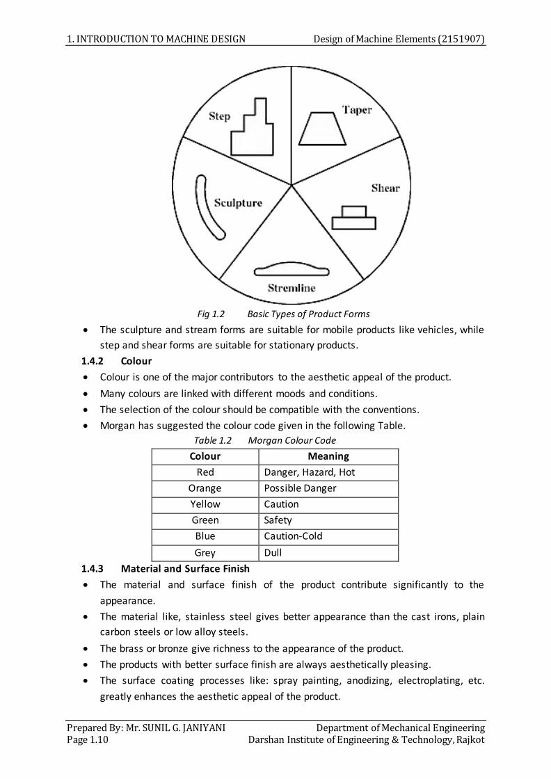
1.4.1 Form (Shape) :
There are five basic forms of the products, namely, step, taper, shear, streamline and
sculpture, as shown in Figure.
The external shape of any product is based on one or combination of these basic
forms.
(i) Step form:
The step form is a stepped structure having vertical accent.
It is similar to the shape of a multistorey building.
(ii) Taper form:
The taper form consists of tapered blocks or tapered cylinders.
(iii) Shear form:
The shear form has a square outlook.
(iv) Streamline form:
The streamline form has a streamlined shape having a smooth flow as seen in
automobile and aeroplane structures.
(v) Sculpture form:
The sculpture form consists of ellipsoids, paraboloids and hyperboloids.
1. INTRODUCTION TO MACHINE DESIGN Design of Machine Elements (2151907)
Prepared By: Mr. SUNIL G. JANIYANI Department of Mechanical Engineering Page 1.10 Darshan Institute of Engineering & Technology, Rajkot
Fig 1.2 Basic Types of Product Forms
The sculpture and stream forms are suitable for mobile products like vehicles, while
step and shear forms are suitable for stationary products.
1.4.2 Colour
Colour is one of the major contributors to the aesthetic appeal of the product.
Many colours are linked with different moods and conditions.
The selection of the colour should be compatible with the conventions.
Morgan has suggested the colour code given in the following Table.
Table 1.2 Morgan Colour Code
Colour Meaning
Red Danger, Hazard, Hot
Orange Possible Danger
Yellow Caution
Green Safety
Blue Caution-Cold
Grey Dull
1.4.3 Material and Surface Finish
The material and surface finish of the product contribute significantly to the
appearance.
The material like, stainless steel gives better appearance than the cast irons, plain
carbon steels or low alloy steels.
The brass or bronze give richness to the appearance of the product.
The products with better surface finish are always aesthetically pleasing.
The surface coating processes like: spray painting, anodizing, electroplating, etc.
greatly enhances the aesthetic appeal of the product.

Design of Machine Elements (2151907) 1. INTRODUCTION TO MACHINE DESIGN
Department of Mechanical Engineering Prepared By: Mr. SUNIL G. JANIYANI Darshan Institute of Engineering & Technology, Rajkot Page 1.11
1.5 Ergonomic Considerations
Ergonomics is defined as the scientific study of the man-machine-working
environment relationship and the application of anatomical, physiological and
psychological principles to solve the problems arising from this relationship.
The word ‘ergonomics’ is formed from two Greek words: ‘ergon’ (work) and ‘nomos’
(natural laws).
The final objective of the ergonomics is to make the machine fit for user rather than
to make the user adapt himself or herself to the machine.
It aims at decreasing the physical and mental stresses to the user.
Psychology - Experimental psychologists who study people at work to provide data
on such things as: Human sensory capacities, psychomotor performance, Human
decision making, Human error rates, Selection tests and procedures, Learning and
training.
Anthropometry - An applied branch of anthropology concerned with the
measurement of the physical features of people. Measures how tall we are, how far
we can reach, how wide our hips are, how our joints flex, and how our bodies move.
Applied Physiology - Concerns the vital processes such as cardiac function,
respiration, oxygen consumption, and electromyography activity, and the responses
of these vital processes to work, stress, and environmental influences.
1.5.1 Communication Between Man (User) and Machine
Fig 1.3 Man-Machine Closed Loop System
Figure shows the man-machine closed loop system.
The machine has a display unit and a control unit.
A man (user) receives the information from the machine display through the
sense organs.
He (or she) then takes the corrective action on the machine controls using
the hands or feet.
This man-machine closed loop system in influenced by the working
environmental factors such as: lighting, noise, temperature, humidity, air
circulation, etc.

1. INTRODUCTION TO MACHINE DESIGN Design of Machine Elements (2151907)
Prepared By: Mr. SUNIL G. JANIYANI Department of Mechanical Engineering Page 1.12 Darshan Institute of Engineering & Technology, Rajkot
1.5.2 Ergonomic Considerations in Design of Displays:
The basic objective in the design of the displays is to minimize the fatigue to the
user. The ergonomic considerations in the design of the displays are as follows:
The scale should be clear and legible.
The size of the numbers or letters on the scale should be taken appropriate.
The pointer should have a knife-edge with a mirror in a dial to minimize the
parallax error while taking the readings.
The scale should be divided in a linear progression such as 0 – 10 – 20 – 30…
and not as 0 – 5 – 25 – 45…..
The number of subdivisions between the numbered divisions should be as
less as possible.
The numbering should be in clockwise direction on a circular scale, from left
to right on a horizontal scale and from bottom to top on a vertical scale.
Fig 1.4 Examples of Displays
1.5.3 Ergonomic Considerations in Design of Controls:
The ergonomic considerations in the design of the controls are as follows:
The control devices should be logically positioned and easily accessible.
The control operation should involve minimum and smooth moments.
The control operation should consume minimum energy.
The portion of the control device which comes in contact with user's hand
should be in conformity with the anatomy of human hands.
The proper colours should be used for control devices and backgrounds so as
to give the required psychological effect.
The shape and size of the control device should be such that the user is
encouraged to handle it in such a way as to exert the required force, but not
excessive force, damaging the control or the machine.
1.5.4 Working Environment
The working environment affects significantly the man-machine relationship.
It affects the efficiency and possibly the health of the operator. The major
working environmental factors are discussed below:
Lighting:
The amount of light that is required to enable a task to be performed
effectively depends upon the nature of the task, the cycle time, the reflective
characteristics of the equipment involved and the vision of the operator.
The intensity of light in the surrounding area should be less than that at the
task area. This makes the task area the focus of attention.

Design of Machine Elements (2151907) 1. INTRODUCTION TO MACHINE DESIGN
Department of Mechanical Engineering Prepared By: Mr. SUNIL G. JANIYANI Darshan Institute of Engineering & Technology, Rajkot Page 1.13
Operators will become less tired if the lighting and colour schemes are
arranged so that there is a gradual change in brightness and colour from the
task area to the surroundings.
The task area should be located such that the operator can occasionally relax
by looking away from the task area towards a distinct object or surface.
The distinct object or surface should not be so bright that the operator's eyes
take time to adjust to the change when he or she again looks at the task.
Glare often causes discomfort and also reduces visibil ity, and hence it should
be minimized or if possible eliminated by careful design of the lighting
sources and their positions.
Noise:
The noise at the work place causes annoyance, damage to hearing and
reduction of work efficiency.
The high pitched noises are more annoying than the low pitched noises.
Noise caused by equipment that a person is using is less annoying than that
caused by the equipment, being used by another person, because the person
has the option of stopping the noise caused by his own equipment, at least
intermittently.
The industrial safety rules specify the acceptable noise levels for different
work places.
If the noise level is too high, it should be reduced at the source by
maintenance, by the use of silencers and by placing vibrating equipment on
isolating mounts.
Further protection can be obtained by placing the sound-insulating walls
around the equipment.
If required, ear plugs should be provided to the operators to reduce the
effect of noise.
Temperature:
For an operator to perform the task efficiently, he should neither feel hot nor
cold.
When the heavy work is done, the temperature should be relatively lower
and when the light work is done, the temperature should be relatively higher.
The optimum required temperature is decided by the nature of the work.
The deviation of the temperature from the optimum temperature required
reduces the efficiency of the operator.
Humidity and air circulation:
Humidity has little effect on the efficiency of the operator at ordinary
temperatures. However, at high temperatures, it affects significantly the
efficiency of the operator.

1. INTRODUCTION TO MACHINE DESIGN Design of Machine Elements (2151907)
Prepared By: Mr. SUNIL G. JANIYANI Department of Mechanical Engineering Page 1.14 Darshan Institute of Engineering & Technology, Rajkot
At high temperatures, the low humidity may cause discomfort due to drying
of throat and nose and high humidity may cause discomfort due to sensation
of stuffiness and over sweating in an ill-ventilated or crowded room.
The proper air circulation is necessary to minimize the effect of high
temperature and humidity.
1.6 Manufacturing considerations in Design or Design for Manufacturing and Assembly
(DFMA)
The design effort makes up only 5 % of the total cost of a product.
However, it usually determines more than 70% of the manufacturing cost of the
product.
Hence, only 30 % of the product’s cost can be changed once the design is finalised
and drawings are prepared.
So the best strategy to lower product cost is to recognize the importance of
manufacturing early in the design stage.
It starts with the formation of the design team which tends to be multi-disciplinary,
including engineers, manufacturing managers, cost accountants, and marketing and
sales professionals.
The most basic approach to design for manufacturing and assembly is to apply
design guidelines.
We should use design guidelines with an understanding of design goals.
Make sure that the application of a guideline improves the design concept on those
goals.
Benefits of DFMA
Design for manufacturing and assembly are simple guidelines formulated to get the
below benefits.
It simplifies the design.
It simplifies the production processes and decreases the product cost.
It improves product quality and reliability (because if the production process
is simplified, then there is less opportunity for errors).
It decreases the assembly cost.
It decreases the assembly time.
It reduces time required to bring a new product into market.
1.6.1 Design for Assembly or DFA Guidelines (Assembly Considerations in Design)
1. Reduce the Part Counts:
Design engineers should try for product design that uses the minimum number
of parts.
Fewer parts result in lower costs.
It also makes assembly simpler and fewer chances of defects.
Minimize part count by incorporating multiple functions into single parts.
Design of Machine Elements (2151907) 1. INTRODUCTION TO MACHINE DESIGN
Department of Mechanical Engineering Prepared By: Mr. SUNIL G. JANIYANI Darshan Institute of Engineering & Technology, Rajkot Page 1.15
Several parts could be fabricated by using different manufacturing processes
(sheet metal forming, injection molding etc.).
Fig 1.5 Reduce the Part Counts
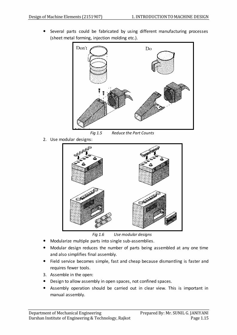
2. Use modular designs:
Fig 1.6 Use modular designs
Modularize multiple parts into single sub-assemblies.
Modular design reduces the number of parts being assembled at any one time
and also simplifies final assembly.
Field service becomes simple, fast and cheap because dismantling is faster and
requires fewer tools.
3. Assemble in the open:
Design to allow assembly in open spaces, not confined spaces.
Assembly operation should be carried out in clear view. This is important in
manual assembly.

1. INTRODUCTION TO MACHINE DESIGN Design of Machine Elements (2151907)
Prepared By: Mr. SUNIL G. JANIYANI Department of Mechanical Engineering Page 1.16 Darshan Institute of Engineering & Technology, Rajkot
Fig 1.7 Assemble in the open
4. Optimize part handling:
Design parts so they do not tangle or stick to each other or require special
handling prior to assembly.
Fig 1.8 Optimize part handling
5. Do not fight gravity:
Design products so that they can be assembled from the bottom to top along
vertical axis.
Design the first part large and wide to be stable and then assemble the smaller
parts on top of it sequentially.
Fig 1.9 Do not fight gravity
6. Design for part identity (symmetry):
Symmetric parts are easy to assemble.
Maximizing part symmetry will make orientation unnecessary.
Features should be added to enhance symmetry wherever required.

Design of Machine Elements (2151907) 1. INTRODUCTION TO MACHINE DESIGN
Department of Mechanical Engineering Prepared By: Mr. SUNIL G. JANIYANI Darshan Institute of Engineering & Technology, Rajkot Page 1.17
7. Eliminate Fasteners:
Fasteners are a major obstacle to efficient assembly and should be avoided
wherever possible.
They are difficult to handle and can cause jamming, if defective.
If the use of fasteners cannot be avoided, limit the number of different types of
fasteners used.
Fig 1.10 Eliminate Fasteners
8. Design parts for simple assembly:
Design parts with orienting features to make alignment easier.
Fig 1.11 Design parts for simple assembly
9. Parts should easily indicate orientation for insertion:
Parts should have self-locking features so that the precise alignment during
assembly is not required or provide marks (color) to make orientation easier.
Don’t Do
Fig 1.12 Parts should easily indicate orientation for insertion

1. INTRODUCTION TO MACHINE DESIGN Design of Machine Elements (2151907)
Prepared By: Mr. SUNIL G. JANIYANI Department of Mechanical Engineering Page 1.18 Darshan Institute of Engineering & Technology, Rajkot
10. Standardize parts to reduce variety:
Using the same commodity items such as fasteners can avoid errors.
It also reduces the cost.
Fig 1.13 Standardize parts to reduce variety
11. Color code parts that are different but shaped similarly:
Distinguish different parts that are shaped similarly by non-geometric means,
such as color coding.
12. Design the mating features for easy insertion:
Add chamfers or other features to make parts easier to insert.
Fig 1.14 Design the mating features for easy insertion
13. Provide alignment features:
Fig 1.15 Provide alignment features

Design of Machine Elements (2151907) 1. INTRODUCTION TO MACHINE DESIGN
Department of Mechanical Engineering Prepared By: Mr. SUNIL G. JANIYANI Darshan Institute of Engineering & Technology, Rajkot Page 1.19
14. Place fasteners away from obstructions:
It is better to locate fasteners in place where one has access to the fastener.
Fig 1.16 Place fasteners away from obstructions
15. Deep channels should be sufficiently wide to provide access to fastening tools:
Fig 1.17 Deep channels should be sufficiently wide to provide access to fastening tools
16. Providing flats for uniform fastening and fastening ease:
Do not fasten against angled surfaces.
Fig 1.18 Providing flats for uniform fastening and fastening ease

1. INTRODUCTION TO MACHINE DESIGN Design of Machine Elements (2151907)
Prepared By: Mr. SUNIL G. JANIYANI Department of Mechanical Engineering Page 1.20 Darshan Institute of Engineering & Technology, Rajkot
1.6.2 Design of components for casting
Why casting?
Complex parts which are difficult to machine, are made by the casting process.
Almost any metal can be melted and cast. Most of the sand cast parts are made
of cast iron, aluminum alloys and brass.
The size of the sand casting can be as small as 10 g and as large as 200 x 103 kg.
Sand castings have irregular and grainy surfaces and machining is required if the
part is moving with respect to some other part or structure.
Cast components are stable, rigid and strong compared with machined or forged
parts.
Typical examples of cast components are machine tool beds and structures,
cylinder blocks of internal combustion engines, pumps and gear box housings.
Basic considerations of casting
Always keep the stressed areas of the parts in compression
Round all external corners
Wherever possible, the section thickness throughout should be held as uniform
as compatible with overall design considerations
Avoid concentration of metal at the junctions
Avoid very thin sections
The wall adjacent to the drilled hole should have a thickness equivalent to the
thickness of the main body
Oval-shaped holes are preferred with larger dimensions along the direction of
forces
To facilitate easy removal, the pattern must have some draft
Outside bosses should be omitted to facilitate a straight pattern draft
(1) Always keep the stressed areas of the parts in compression
Cast iron has more compressive strength than its tensile strength.
The castings should be placed in such a way that they are subjected to
compressive rather than tensile stresses.
Fig 1.19 (a) Incorrect (Part in tension) (b) Correct (Part in compression)

Design of Machine Elements (2151907) 1. INTRODUCTION TO MACHINE DESIGN
Department of Mechanical Engineering Prepared By: Mr. SUNIL G. JANIYANI Darshan Institute of Engineering & Technology, Rajkot Page 1.21
When tensile stresses are unavoidable, a clamping device such as a tie rod or a
bearing cap should be considered.
The clamping device relieves the cast iron components from tensile stresses.
Fig 1.20 (a) Original component (b) Use of Tie-rod (c) Use of Bearing-cap
(2) Round all external corners
It increases the endurance limit of the component and reduces the formation of
brittle chilled edges.
When the metal in the corner cools faster than the metal adjacent to the corner,
brittle chilled edges are formed.
Appropriate fillet radius reduces the stress concentration.
Fig 1.21 Round all external corners
(3) Wherever possible, the section thickness throughout should be held as uniform
as compatible with overall design considerations
Abrupt changes in the cross-section result in high stress concentration.
If the thickness is to be varied at all, the change should be gradual

1. INTRODUCTION TO MACHINE DESIGN Design of Machine Elements (2151907)
Prepared By: Mr. SUNIL G. JANIYANI Department of Mechanical Engineering Page 1.22 Darshan Institute of Engineering & Technology, Rajkot
Fig 1.22 Uniform thickness throughout
(4) Avoid concentration of metal at the junctions
At the junction, there is a concentration of metal.
Even after the metal on the surface solidifies, the central portion still remains in
the molten stage, with the result that a shrinkage cavity or blowhole may appear
at the centre.
There are two ways to avoid the concentration of metal.
One is to provide a cored opening in webs and ribs.
Alternatively, one can stagger the ribs and webs.
Fig 1.23 Cored Holes
Fig 1.24 Staggered ribs
Design of Machine Elements (2151907) 1. INTRODUCTION TO MACHINE DESIGN
Department of Mechanical Engineering Prepared By: Mr. SUNIL G. JANIYANI Darshan Institute of Engineering & Technology, Rajkot Page 1.23
(5) Avoid very thin sections
It depends upon the process of casting such as sand casting , permanent mold
casting or die casting
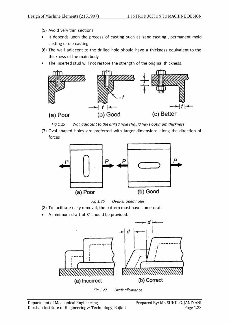
(6) The wall adjacent to the drilled hole should have a thickness equivalent to the
thickness of the main body
The inserted stud will not restore the strength of the original thickness.
Fig 1.25 Wall adjacent to the drilled hole should have optimum thickness
(7) Oval-shaped holes are preferred with larger dimensions along the direction of
forces
Fig 1.26 Oval-shaped holes
(8) To facilitate easy removal, the pattern must have some draft
A minimum draft of 3° should be provided.
Fig 1.27 Draft allowance

1. INTRODUCTION TO MACHINE DESIGN Design of Machine Elements (2151907)
Prepared By: Mr. SUNIL G. JANIYANI Department of Mechanical Engineering Page 1.24 Darshan Institute of Engineering & Technology, Rajkot
(9) Outside bosses should be omitted to facilitate a straight pattern draft
Fig 1.28 Outside bosses should be omitted
1.6.3 Design of components for Forging
Why forging?
A properly designed forging is not only sound with regard to strength but it also
helps reduce the forging forces, improves die life and simplifies die design.
Forged components are usually made of steels and non-ferrous metals.
They can be as small as a gudgeon pin and as large as a crankshaft.
Forged components are used under the following circumstances:
i. Moving components requiring light weight to reduce inertia forces, e.g.
connecting rod of I. C. engines.
ii. Components subjected to excessive stresses, e.g. aircraft structures.
iii. Small components that must be supported by other structures or parts, e.g.
hand tools and handles.
iv. Components requiring pressure tightness where the part must be free from
internal cracks, e.g. valve bodies.
v. Components whose failure would cause injury and expens ive damage are
forged for safety.
Basic considerations of Forging
While designing a forging, advantage should be taken of the direction of fibre
lines
The forged component should be provided with an adequate draft
The parting line should be in one plane as far as possible and it should divide the
forging into two equal parts
The forging should be provided with adequate fillet and corner radius
Thin sections and ribs should be avoided in forged components

Design of Machine Elements (2151907) 1. INTRODUCTION TO MACHINE DESIGN
Department of Mechanical Engineering Prepared By: Mr. SUNIL G. JANIYANI Darshan Institute of Engineering & Technology, Rajkot Page 1.25
(1) While designing a forging, advantage should be taken of the direction of fibre
lines
Fig 1.29 Direction of fibre lines
There are no fibre lines in the cast component and the grains are scattered.
In case of a component prepared by machining methods, such as turning or
milling, the original fibre lines of rolled stock are broken.
It is only in case of forged parts that the fibre lines are arranged in a favorable
way to withstand stresses due to external load.
While designing a forging, the profile is selected in such a way that fibre lines are
parallel to tensile forces and perpendicular to shear forces.
(2) The forged component should be provided with an adequate draft
The draft angle is provided for an easy removal of the part from the die
impressions.
Fig 1.30 Provision of Draft
(3) The parting line should be in one plane as far as possible and it should divide the
forging into two equal parts
When the parting line is broken, it results in unbalanced forging forces, which
tends to displace the two die halves.

1. INTRODUCTION TO MACHINE DESIGN Design of Machine Elements (2151907)
Prepared By: Mr. SUNIL G. JANIYANI Department of Mechanical Engineering Page 1.26 Darshan Institute of Engineering & Technology, Rajkot
Fig 1.31 Parting line consideration
(4) The forging should be provided with adequate fillet and corner radius
Sharp corners result in increasing difficulties in filling the material, excessive
forging forces, and poor die life.
The magnitude of fillet radius depends upon the material, the size of forging and
the depth of the die cavity.
(5) Thin sections and ribs should be avoided in forged components
A thin section cools at a faster rate in the die cavity and requires excessive force
for plastic deformation.
It reduces the die life, and the removal of the component from the die cavities
becomes difficult.
1.6.4 Design of components for Welding
Why welding?
Welding is the most important method of joining the parts into a complex
assembly.
Basic considerations of Welding
Select the Material with High Weldability
Use Minimum Number of Welds
Use Standard Components
Select Proper Location for the Weld
Prescribe Correct Sequence of Welding
Reduce Edge Preparation
Reduce the Scrap
Avoid Weld Accumulation
(1) Select the Material with High Weldability
In general, low carbon steel is more easily welded than high carbon steel.
Higher carbon content tends to harden the welded joint, as a result of which the
weld is susceptible to cracks.
(2) Use Minimum Number of Welds
Only the adjoining area of the joint is heated up, which has no freedom to
expand or contract.

Design of Machine Elements (2151907) 1. INTRODUCTION TO MACHINE DESIGN
Department of Mechanical Engineering Prepared By: Mr. SUNIL G. JANIYANI Darshan Institute of Engineering & Technology, Rajkot Page 1.27
Uneven expansion and contraction in this adjoining area and parent metal results
in distortion.
Since distortion always occurs in welding, the design should involve a minimum
number of welds and avoid over welding.
It will not only reduce the distortion but also the cost.
(3) Use Standard Components
The designer should specify standard sizes for plates, bars and rolled sections.
Non-standard sections involve flame cutting of plates and additional welding.
As far as possible, the designer should select plates of equal thickness for a butt
joint.
(4) Select Proper Location for the Weld
The welded joint should be located in an area where stresses and deflection are
not critical.
Also, it should be located at such a place that the welder and welding machine
has unobstructed access to that location.
(5) Prescribe Correct Sequence of Welding
The designer should consider the sequence in which the parts should be welded
together for minimum distortion.
This is particularly important for a complex job involving a number of welds.
An incorrect sequence of welding causes distortion and sometimes cracks in the
weld metal due to stress concentration at some point in fabrication.
A correct welding sequence distributes and balances the forces and stresses
induced by weld contraction.
(6) Reduce edge preparation
It is necessary to prepare bevel edges for the components prior to welding
operation.
This preparatory work can be totally eliminated by making a slight change in the
arrangement of components.
(a) Incorrect (b) Correct
Fig 1.32 Reduce edge preparation

1. INTRODUCTION TO MACHINE DESIGN Design of Machine Elements (2151907)
Prepared By: Mr. SUNIL G. JANIYANI Department of Mechanical Engineering Page 1.28 Darshan Institute of Engineering & Technology, Rajkot
(7) Reduce the scrap
Many times, fabrication is carried out by cutting steel plates followed by welding.
The aim of the designer is to minimize scrap in such process.
The circular top plate and annular bottom plate are cut from two separate plates
resulting in excess scrap as shown in Figure.
Making a slight change in design, the top plate and annual bottom plate can be
cut from one plate reducing scrap and material cost.
Fig 1.33 Reduce the scrap
(8) Avoid Weld Accumulation
Accumulation of welded joints results in shrinkage stresses.
Fig 1.34 Avoid Weld Accumulation
1.6.5 Design of components for Machining
Why machining?
Machined components are widely used in all industrial products.
They are usually made from ferrous and non-ferrous metals.
They are as small as a gear in a wristwatch and as large as huge turbine housing.
Metal-cutting operations: Turning, Milling, drilling, shaping, boring, reaming etc.
Surface finishing operations: Grinding, buffing etc.
Machined components are used under the following circumstances:
i. Components requiring precision and high dimensional accuracy
ii. Components requiring flatness, roundness, parallelism or circularity for
their proper functioning
iii. Components of interchangeable assembly
iv. Components, which are in relative motion with each other or with some
fixed part

Design of Machine Elements (2151907) 1. INTRODUCTION TO MACHINE DESIGN
Department of Mechanical Engineering Prepared By: Mr. SUNIL G. JANIYANI Darshan Institute of Engineering & Technology, Rajkot Page 1.29
Basic considerations of Machining
Avoid Machining
Specify Liberal Tolerances
Avoid Sharp Corners
Use Stock Dimensions
Design Rigid Parts
Avoid Shoulders and undercuts
Avoid Hard Materials
Design machined parts with features that can be produced in a minimum number
of setups
Machine only functional surface
Holes should be parallel or perpendicular to the axis of the part
Design holes with conical ends
Use minimum number of machines
Design the product for existing machining facilities
Machining should be completed in minimum machining operations
Use standard size tooling
Avoid parts with very large L/D ratios
Machined surfaces should be parallel or perpendicular to each other as well as to
base
(1) Avoid Machining
Machining operations increase cost of the component.
Components made by casting or forming methods are usually cheaper.
Therefore, as far as possible, the designer should avoid machined surfaces.
(2) Specify Liberal Tolerances
The secondary machining operations like grinding or reaming are costly.
Therefore, depending upon the functional requirement of the component, the
designer should specify the most liberal dimensional and geometric tolerances.
Closer the tolerance, higher is the cost.
(3) Avoid Sharp Corners
The Sharp corners result in stress concentration. Therefore, the designer should
avoid shapes that require sharp corners.
(4) Use Stock Dimensions
Raw materials like bars are available in standard sizes.
Using stock dimensions eliminates machining operations.
For example, a hexagonal bar can be used for a bolt and only the threaded
portion can be machined. This will eliminate machining of hexagonal surfaces.
(5) Design Rigid Parts
Any machining operation such as turning or shaping induces cutting forces on the
components.

1. INTRODUCTION TO MACHINE DESIGN Design of Machine Elements (2151907)
Prepared By: Mr. SUNIL G. JANIYANI Department of Mechanical Engineering Page 1.30 Darshan Institute of Engineering & Technology, Rajkot
The component should be rigid enough to withstand these forces.
In this respect, components with thin walls or webs should be avoided.
(6) Avoid Shoulders and undercuts
Shoulders and undercuts usually involve separate operations and separate tools,
which increase the cost of machining.
(7) Avoid Hard Materials
Hard materials are difficult to machine.
They should be avoided unless such properties are essential for the functional
requirement of the Product.
(8) Design machined parts with features that can be produced in a minimum
number of setups
Fig 1.35 Minimum number of setups
(9) Machine only functional surface
Fig 1.36 Machine only functional surface
1.6.6 Design for Creep (Thermal Considerations in Design)
Creep is defined as slow and progressive deformation of the material with time
under a constant stress.
Creep deformation is a function of stress level and temperature.
Therefore, creep deformation is higher at higher temperature and creep
becomes important for components operating at high temperatures.
Deformation due to creep must remain within permissible limit and rupture must
not occur during the service life.
Most of the machine elements are used in engineering applications which
operate at ordinary temperatures.
Some applications where machine elements are subjected to high temperatures :
I. C. Engines, Turbines, Boilers, Pressure Vessels in process industries etc.
The rate of deformation is called the creep rate.
It is the slope of the line in a curve of Creep strain vs. Time.
Strain is deformation per unit length.

Design of Machine Elements (2151907) 1. INTRODUCTION TO MACHINE DESIGN
Department of Mechanical Engineering Prepared By: Mr. SUNIL G. JANIYANI Darshan Institute of Engineering & Technology, Rajkot Page 1.31
Fig 1.37 Creep Curve
An idealized creep curve is shown in the above figure.
When the load is applied at the beginning of the creep test, the instantaneous
elastic deformation OA occurs.
This elastic deformation is followed by the creep curve ABCD.
Creep occurs in three stages.
(i) Primary Creep
(ii) Secondary Creep
(iii) Tertiary Creep
Primary Creep
The first stage called primary creep is shown by AB on the curve.
During this stage, the creep rate, i.e., the slope of the creep curve from A to B
progressively decreases with time.
Deformation becomes more and more difficult as strain increases, i.e. the
material experiences strain hardening.
The metal strain hardens to support the external load.
Secondary Creep
The second stage called secondary creep is shown by BC on the curve.
During this stage, the creep rate is constant.
This stage occupies a major portion of the life of the component. The designer is
mainly concerned with this stage.
The occurrence of a constant strain-rate is explained in terms of a balance
between strain hardening and structure recovery (a softening process
determined by the high temperature).
Tertiary Creep
The third stage called tertiary creep is shown by CD on the creep curve.
During this stage, the creep rate is accelerated due to necking and also due to
formation of voids along the grain boundaries.
Therefore, creep rate rapidly increases and finally results in fracture at the point
D.

1. INTRODUCTION TO MACHINE DESIGN Design of Machine Elements (2151907)
Prepared By: Mr. SUNIL G. JANIYANI Department of Mechanical Engineering Page 1.32 Darshan Institute of Engineering & Technology, Rajkot
(a) Initial state
(b) After 100 000 h
Fig 1.38 Creep test
Creep properties are determined by experiments and these experiments involve
very long periods stretching into months.
Fig 1.39 Creep Failure
Design Considerations to avoid Creep
1. Select material which gives good performance at high temperatures.
2. The component must be designed considering operating temperatures.
3. Use large grains or mono-crystals (small grains increase grain motion at the
grain boundaries)
4. Addition of solid solutions to eliminate vacancies.
5. Consult creep test data during materials selection.

Design of Machine Elements (2151907) 1. INTRODUCTION TO MACHINE DESIGN
Department of Mechanical Engineering Prepared By: Mr. SUNIL G. JANIYANI Darshan Institute of Engineering & Technology, Rajkot Page 1.33
1.6.7 Design for Wear (Wear Considerations in Design)
Wear
Wear can be defined as the progressive loss or removal of material from the
surfaces in contact, as a result of the relative motion.
Wear is not a material property but it is a response of the engineering system.
Effects of Wear
It distorts the original geometry and surface finish of the machine elements.
It increases the clearance between the mating parts, resulting in additional load,
vibrations and noise.
It reduces the functionality of the machine elements.
It reduces the life of the machine elements and machine.
It damages the machine elements and machine.
Therefore, wear is one of the important design considerations while designing
any machine element.
Applications where Wear is Undesirable
Gears, Brakes, Clutches, Tyres, Piston and cylinder, Cam and follower, Bearings
etc.
Applications where Wear is Desirable
Machining, Grinding, Writing with pencils etc.
Design Considerations for Wear
1. Proper lubrication
2. Surface coating
3. Surface hardening
4. Reducing the surface roughness of the contacting surfaces
5. Sealing the contact areas to avoid the foreign abrasive particles.
1.6.8 Contact Stresses (or Hertz contact stress)
Hertz Contact Stress
The theoretical contact area of two spheres is a point.
The theoretical contact area of two parallel cylinders is a line.
In reality, a small contact area is being created through elastic deformation,
thereby inducing the stresses considerably.
These contact stresses are called Hertz contact stresses.
Fig 1.40 Gear tooth Failure Due to Hertz Contact Stress

1. INTRODUCTION TO MACHINE DESIGN Design of Machine Elements (2151907)
Prepared By: Mr. SUNIL G. JANIYANI Department of Mechanical Engineering Page 1.34 Darshan Institute of Engineering & Technology, Rajkot
Two design cases will be considered.
1. Sphere – Sphere Contact
(a) Two spheres held in contact by force F
(b) Contact stress has an elliptical distribution across contact over zone of diameter 2a
Fig 1.41 Sphere – Sphere Contact
The theoretical contact area of two spheres is a point.
Consider two solid elastic spheres held in contact by a force F such that their
point of contact expands into a circular area of radius a, given as, √
where [
( )
(
)
]
F = applied force
v1, v2 = Poisson’s ratio for spheres 1 and 2 respectively
E1, E2 = Young’s modulus for spheres 1 and 2 respectively
d1, d2 = Diameters for spheres 1 and 2 respectively
The maximum contact stress (σCH) occurs at the center point of the contact area
and it is given by,
2. Cylinder – Cylinder Contact
(a) Two right circular cylinders held in contact by force F uniformly distributed along length l
(b) Contact stress has an elliptical distribution across contact over zone of width 2b
Fig 1.42 Cylinder – Cylinder Contact

Design of Machine Elements (2151907) 1. INTRODUCTION TO MACHINE DESIGN
Department of Mechanical Engineering Prepared By: Mr. SUNIL G. JANIYANI Darshan Institute of Engineering & Technology, Rajkot Page 1.35
The theoretical contact area of two parallel cylinders is a line.
Consider two solid elastic cylinders held in contact by forces F uniformly
distributed along the cylinder length l.
The resulting pressure causes the line of contact to become a rectangular
contact zone of half width b given as, √
where [
( )
(
)
]
F = applied force
v1, v2 = Poisson’s ratio for cylinders 1 and 2 respectively
E1, E2 = Young’s modulus for cylinders 1 and 2 respectively
d1, d2 = Diameters for cylinders 1 and 2 respectively
l = Length for cylinders (l1, = l2 assumed)
The maximum contact stress (σCH) between the cylinders acts along a
longitudinal line at the center of the rectangular contact area, and is computed
as
1.7 Material Selection in Machine Design
Selection of a proper material for the machine component is one of the most
important steps in the process of machine design.
The best material is one which will serve the desired purpose at minimum cost.
It is not always easy to select such a material and the process may involve the trial
and error method.
The factors which should be considered while selecting the material for a machine
component are as follows:
1. Availability
2. Cost
3. Mechanical Properties
4. Manufacturing Considerations
1. Availability:
The material should be readily available in the market, in large enough
quantities to meet the requirement.
Cast iron and aluminium alloys are always available in abundance while
shortage of lead and copper alloys is a common experience.
2. Cost:
Cost For every application, there is a limiting cost beyond which the designer
cannot go.
When the limit is exceeded, the designer has to consider other alternative
materials.
In cost analysis, there are two factors, namely cost of material and cost of
processing the material into finished goods.

1. INTRODUCTION TO MACHINE DESIGN Design of Machine Elements (2151907)
Prepared By: Mr. SUNIL G. JANIYANI Department of Mechanical Engineering Page 1.36 Darshan Institute of Engineering & Technology, Rajkot
It is likely that the cost of material might be low, but the processing may
involve costly manufacturing operations.
3. Mechanical Properties:
Mechanical properties are the most important technical factor governing the
selection of material.
They include strength under static and fluctuating loads, elasticity, plasticity,
stiffness, resilience, toughness, ductility, malleability and hardness.
Depending upon the conditions and the functional requirement, different
mechanical properties are considered and a suitable material is selected.
The piston rings should have a hard surface to resist wear due to rubbing
action with the cylinder surface, and surface hardness is the selection
criterion.
In case of bearing materials, a low coefficient of friction is des irable while
clutch or brake requires a high coefficient of friction.
4. Manufacturing Considerations:
In some applications, machinability of material is an important consideration
in selection.
Sometimes, an expensive material is more economical than a low priced one,
which is difficult to machine.
Free cutting steels have excellent machinability, which is an important factor
in their selection for high strength bolts, axles and shafts.
Where the product is of complex shape, castability or ability of the molten
metal to flow into intricate passages is the criterion of material selection.
In fabricated assemblies of plates and rods, weldability becomes the
governing factor.
The manufacturing processes, such as casting, forging, extrusion, welding and
machining govern the selection of material.
1.8 Mechanical Properties of Metals
The mechanical properties of the metals are those which are associated with the
ability of the material to resist mechanical forces and load.
1. Strength: It is the ability of a material to resist the externally applied forces
without breaking or yielding.
The internal resistance offered by a part to an externally applied force is
called stress.
2. Stiffness: It is the ability of a material to resist deformation under stress.
The modulus of elasticity is the measure of stiffness.
3. Elasticity: It is the property of a material to regain its original shape after
deformation when the external forces are removed.
This property is desirable for materials used in tools and machines.
It may be noted that steel is more elastic than rubber.

Design of Machine Elements (2151907) 1. INTRODUCTION TO MACHINE DESIGN
Department of Mechanical Engineering Prepared By: Mr. SUNIL G. JANIYANI Darshan Institute of Engineering & Technology, Rajkot Page 1.37
4. Plasticity: It is property of a material which retains the deformation produced
under load permanently.
This property of the material is necessary for forgings, in stamping images on
coins and in ornamental work.
5. Ductility: It is the property of a material enabling it to be drawn into wire with
the application of a tensile force.
The ductility is usually measured by the terms, percentage elongation and
percentage reduction in area.
The ductile material commonly used in engineering practice (in order of
diminishing ductility) are mild steel, copper, aluminium, nickel, zinc, tin and
lead.
6. Malleability: It is a special case of ductility which permits materials to be rolled or
hammered into thin sheets.
The malleable materials commonly used in engineering practice (in order of
diminishing malleability) are lead, soft steel, wrought iron, copper and
aluminium.
7. Brittleness: It is the property of a material opposite to ductility. It is the property
of breaking of a material with little permanent distortion.
Brittle materials when subjected to tensile loads, it snaps off without giving
any sensible elongation.
Cast iron is a brittle material.
8. Toughness: It is the property of a material to resist fracture due to high impact
loads like hammer blows.
The toughness of the material decreases when it is heated.
It is measured by the amount of energy that a unit volume of the material has
absorbed after being stressed upto the point of fracture.
This property is desirable in parts subjected to shock and impact loads.
9. Machinability: It is the property of a material which refers to a relative case with
which a material can be cut.
10. Resilience: It is the property of a material to absorb energy and to resist shock
and impact loads.
It is measured by the amount of energy absorbed per unit volume within
elastic limit.
This property is essential for spring materials.
11. Creep: When a part is subjected to a constant stress at high temperature for a
long period of time, it will undergo a slow and permanent deformation called
creep.
This property is considered in designing internal combustion engines, boilers
and turbines.

1. INTRODUCTION TO MACHINE DESIGN Design of Machine Elements (2151907)
Prepared By: Mr. SUNIL G. JANIYANI Department of Mechanical Engineering Page 1.38 Darshan Institute of Engineering & Technology, Rajkot
12. Fatigue: When a material is subjected to repeated stresses, it fails at stresses
below the yield point stresses. Such type of failure of a material is known as
fatigue.
The failure is caused by means of a progressive crack formation which are
usually fine and of microscopic size.
This property is considered in designing shafts, connecting rods, springs,
gears, etc.
13. Hardness: It is a very important property of the metals and has a wide variety of
meanings.
It embraces many different properties such as resistance to wear, scratching,
deformation and machinability etc.
It also means the ability of a metal to cut another metal.
The hardness is usually expressed in numbers which are dependent on the
method of making the test.
The hardness of a metal may be determined by the following tests:
(a) Brinell hardness test, (b) Rockwell hardness test,
(c) Vickers hardness test and (d) Shore scleroscope.
1.9 Effect of Impurities on Steel
The following are the effects of impurities like silicon, sulphur, manganese and
phosphorus on steel.
1. Silicon: The amount of silicon in the finished steel usually ranges from 0.05 to
0.30%.
Silicon is added in low carbon steels to prevent them from becoming porous.
It removes the gases and oxides, prevent blow holes and thereby makes the
steel tougher and harder.
2. Sulphur: It occurs in steel either as iron sulphide or manganese sulphide.
Iron sulphide because of its low melting point produces red shortness,
whereas manganese sulphide does not affect so much.
Therefore, manganese sulphide is less objectionable in steel than iron
sulphide.
3. Manganese: It serves as a valuable deoxidizing and purifying agent in steel .
Manganese also combines with sulphur and thereby decreases the harmful
effect of this element remaining in the steel.
When used in ordinary low carbon steels, manganese makes the metal
ductile and of good bending qualities.
In high speed steels, it is used to toughen the metal and to increase its critical
temperature.
4. Phosphorus: It makes the steel brittle.
It also produces cold shortness in steel.

Design of Machine Elements (2151907) 1. INTRODUCTION TO MACHINE DESIGN
Department of Mechanical Engineering Prepared By: Mr. SUNIL G. JANIYANI Darshan Institute of Engineering & Technology, Rajkot Page 1.39
In low carbon steels, it raises the yield point and improves the resistance to
atmospheric corrosion.
The sum of carbon and phosphorus usually does not exceed 0.25%.
1.10 Effects of Alloying Elements on Steel
Alloy steel may be defined as steel to which elements other than carbon are added
in sufficient amount to produce an improvement in properties.
The alloying is done for specific purposes to increase wearing resistance, corrosion
resistance and to improve electrical and magnetic properties, which cannot be
obtained in plain carbon steels.
The chief alloying elements used in steel are nickel, chromium, molybdenum, cobalt,
vanadium, manganese, silicon and tungsten.
These elements may be used separately or in combination to produce the desired
characteristic in steel.
1. Nickel: It increases the strength and toughness of the steel.
These steels contain nickel from 2 to 5% and carbon from 0.1 to 0.5%.
In this range, nickel contributes great strength and hardness with high elastic
limit, good ductility and good resistance to corrosion.
An alloy containing 25% nickel possesses maximum toughness and offers the
greatest resistance to rusting, corrosion and burning at high temperature.
It has proved to be of advantage in the manufacture of boiler tubes, valves
for use with superheated steam, valves for I. C. engines and spark plugs for
petrol engines.
A nickel steel alloy containing 36% of nickel is known as invar. It has nearly
zero coefficient of expansion. So it is in great demand for measuring
instruments and standards of lengths for everyday use.
2. Chromium: It is used in steels as an alloying element to combine hardness with
high strength and high elastic limit.
It also imparts corrosion-resisting properties to steel.
The most common chrome steels contains from 0.5 to 2% chromium and 0.1
to 1.5% carbon.
The chrome steel is used for balls, rollers and races for bearings.
A nickel chrome steel containing 3.25% nickel, 1.5% chromium and 0.25%
carbon is much used for armor plates.
Chrome nickel steel is extensively used for motor car crankshafts, axles and
gears requiring great strength and hardness.
3. Vanadium: It aids in obtaining a fine grain structure in tool steel.
The addition of a very small amount of vanadium (less than 0.2%) produces a
marked increase in tensile strength and elastic limit in low and medium
carbon steels without a loss of ductility.

1. INTRODUCTION TO MACHINE DESIGN Design of Machine Elements (2151907)
Prepared By: Mr. SUNIL G. JANIYANI Department of Mechanical Engineering Page 1.40 Darshan Institute of Engineering & Technology, Rajkot
The chrome-vanadium steel, containing about 0.5 to 1.5% chromium, 0.15 to
0.3% Vanadium and 0.13 to 1.1% carbon have extremely good tensile
strength, elastic limit, endurance limit and ductility.
These steels are frequently used for parts such as springs, shafts, gears, pins
and many drop forged parts.
4. Tungsten: It prohibits grain growth, increases the depth of hardening of quenched
steel and confers the property of remaining hard even when heated to red colour.
It is usually used in conjunction with other elements.
Steel containing 3 to 18% tungsten and 0.2 to 1.5% carbon is used for cutting
tools.
The principal uses of tungsten steels are for cutting tools, dies, valves, taps
and permanent magnets.
5. Cobalt: It gives red hardness by retention of hard carbides at high temperatures.
It tends to decarburise steel during heat-treatment.
It increases hardness and strength and also residual magnetism and coercive
magnetic force in steel for magnets.
6. Manganese. It improves the strength of the steel in both the hot rolled and heat
treated condition.
The manganese alloy steels containing over 1.5% manganese with a carbon
range of 0.40 to 0.55% are used extensively in gears, axles, shafts and other
parts where high strength combined with fair ductility is required.
The principal use of manganese steel is in machinery parts subjected to
severe wear. These steels are all cast and ground to finish.
7. Silicon: The silicon steels behave like nickel steels.
These steels have a high elastic limit as compared to ordinary carbon steel.
Silicon steels containing from 1 to 2% silicon and 0.1 to 0.4% carbon and
other alloying elements are used for electrical machinery, valves in I. C.
engines, springs and corrosion resisting materials.
8. Molybdenum: A very small quantity (0.15 to 0.30%) of molybdenum is generally
used with chromium and manganese (0.5 to 0.8%) to make molybdenum steel.
These steels possess extra tensile strength and are used for air-plane fuselage
and automobile parts.
It can replace tungsten in high speed steels.
1.11 Heat Treatment of Steels
It can be defined as an operation or a combination of operations, involving the
heating and cooling of a metal or an alloy in the solid state for the purpose of
obtaining certain desirable conditions or properties without change in chemical
composition.
The aim of heat treatment is to achieve one or more of the following objects:
1. To increase the hardness of metals.

Design of Machine Elements (2151907) 1. INTRODUCTION TO MACHINE DESIGN
Department of Mechanical Engineering Prepared By: Mr. SUNIL G. JANIYANI Darshan Institute of Engineering & Technology, Rajkot Page 1.41
2. To relieve the stresses set up in the material after hot or cold working.
3. To improve machinability.
4. To soften the metal.
5. To modify the structure of the material to improve its electrical and magnetic
properties.
6. To change the grain size.
Following are the various heat treatment processes commonly employed in
engineering practice are as follow:
1. Normalising
2. Annealing
(a) Full annealing
(b) Process annealing
3. Spheroidising
4. Hardening
5. Tempering
6. Surface hardening or case hardening

Department of Mechanical Engineering Prepared By: Mr. SUNIL G. JANIYANI Darshan Institute of Engineering & Technology, Rajkot Page 2.1
2 DESIGN AGAINST FLUCTUATING LOADS
Course Contents
2.1 Stress Concentration
2.2 Fatigue
2.3 Factors Affecting Endurance
Strength
2.4 Design for Reversed Stresses
2.5 Design for Fluctuating
Stresses
2.6 Modified Goodman Diagrams
Examples

2. DESIGN AGAINST FLUCTUATING LOADS Design of Machine Elements (2151907)
Prepared By: Mr. SUNIL G. JANIYANI Department of Mechanical Engineering Page 2.2 Darshan Institute of Engineering & Technology, Rajkot
2.1 Stress Concentration
It is defined as the localization of high stresses due to the irregularities present in the
component and abrupt changes of the cross-section.
A plate with a small circular hole, subjected to tensile stress is shown in Fig. 2.1.
The localized stresses in the neighborhood of the hole are far greater.
Fig 2.1 Stress Concentration
2.1.1 Causes of Stress Concentration
1. Variation in Properties of Materials:
In design of machine components, it is assumed that the material is
homogeneous throughout the component.
In practice, there is variation in material properties from one end to another
due to the following factors:
(a) Internal cracks and flaws like blow holes;
(b) Cavities in welds;
(c) Air holes in steel components; and
(d) Nonmetallic or foreign inclusions.
These variations act as discontinuities in the component and cause stress
concentration.
2. Load Application:
Machine components are subjected to forces.
These forces act either at a point or over a small area of the component.
Since the area is small, the pressure at these points is excessive. This results
in stress concentration.
The examples of these load applications are as follows:
(a) Contact between the meshing teeth of the driving and the driven gear

Design of Machine Elements (2151907) 2. DESIGN AGAINST FLUCTUATING LOADS
Department of Mechanical Engineering Prepared By: Mr. SUNIL G. JANIYANI Darshan Institute of Engineering & Technology, Rajkot Page 2.3
(b) Contact between the cam and the follower
(c) Contact between the balls and the races of ball bearing
(d) Contact between the rail and the wheel
(e) Contact between the crane hook and the chain
In all these cases, the concentrated load is applied over a very small area
which results in stress concentration.
3. Abrupt Changes in Section:
In order to mount gears, sprockets, pulleys and ball bearings on a
transmission shaft, steps are cut on the shaft and shoulders are provided
from assembly considerations.
Although these features are essential, they create change of the cross -section
of the shaft.
This results in stress concentration at these cross-sections.
Fig 2.2 Abrupt Changes in Section
4. Discontinuities in the Component:
Certain features of machine components such as oil holes or oil grooves,
keyways and splines, and screw threads result in discontinuities in the cross -
section of the component.
There is stress concentration in the area of these discontinuities.
5. Machining Scratches:
Machining scratches, stamp marks or inspection marks are surface
irregularities, which cause stress concentration.
2.1.2 Methods to Reduce Stress Concentration
1. Additional Notches and Holes in Tension Member
A flat plate with a V-notch subjected to tensile force is shown in Fig. 2.3 (a).
It is observed that a single notch results in a high degree of stress
concentration.
The severity of stress concentration is reduced by three methods: (a) Use of
multiple notches, (b) Drilling additional holes; and (c) Removal of undesired
material

2. DESIGN AGAINST FLUCTUATING LOADS Design of Machine Elements (2151907)
Prepared By: Mr. SUNIL G. JANIYANI Department of Mechanical Engineering Page 2.4 Darshan Institute of Engineering & Technology, Rajkot
Fig 2.3 Reduction of Stress Concentration due to V-notch: (a) Original Notch (b) Multiple
Notches(c) Drilled Holes (d) Removal of Undesirable Material
These methods are illustrated in Fig. 2.3 (b), (c) and (d) respectively.
In these three methods, the sharp bending of a force flow line is reduced and
it follows a smooth curve.
2. Fillet Radius, Undercutting and Notch for Member in Bending:
Fig 2.4 Reduction of stress Concentration due to Abrupt change in Cross-section: (a) Original
Component (b) Fillet Radius (c)Undercutting (d) Additional Notch
A bar of circular cross-section with a shoulder and subjected to bending
moment is shown in Fig. 2.4 (a).
Ball bearings, gears or pulleys are seated against this shoulder.
The shoulder creates a change in cross-section of the shaft, which results in
stress concentration.
There are three methods to reduce stress concentration at the base of this
shoulder.
Fig. 2.4 (b) shows the shoulder with a fillet radius r. This results in gradual
transition from small diameter to a large diameter.

Design of Machine Elements (2151907) 2. DESIGN AGAINST FLUCTUATING LOADS
Department of Mechanical Engineering Prepared By: Mr. SUNIL G. JANIYANI Darshan Institute of Engineering & Technology, Rajkot Page 2.5
The fillet radius should be as large as possible in order to reduce stress
concentration.
In practice, the fillet radius is limited by the design of mating components.
The fillet radius can be increased by undercutting the shoulder as illustrated
in Fig. 2.4 (c).
A notch results in stress concentration.
Cutting an additional notch is an effective way to reduce stress
concentration. This is illustrated Fig. 2.4 (d).
3. Drilling Additional Holes for Shaft:
Fig 2.5 Reduction of Stress Concentration in Shaft with Keyway: (a) Original Shaft (b) Drilled
Holes (c)Fillet Radius
A transmission shaft with a keyway is shown in Fig. 2.5 (a).
The keyway is a discontinuity and results in stress concentration at the
corners of the keyway and reduces torsional shear strength.
In addition to giving fillet radius at the inner corners of the keyway (as shown
in Fig. 2.5 (c)), there is another method of drilling two symmetrical holes on
the sides of the keyway.
These holes press the force flow lines and minimise their bending in the
vicinity of the keyway. This method is illustrated in Fig. 2.5 (b).
4. Reduction of Stress Concentration in Threaded Members:
A threaded component is shown in Fig. 2.6 (a).
It is observed that the force flow line is bent as it passes from the shank
portion to threaded portion of the component. This results in stress
concentration in the transition plane.

2. DESIGN AGAINST FLUCTUATING LOADS Design of Machine Elements (2151907)
Prepared By: Mr. SUNIL G. JANIYANI Department of Mechanical Engineering Page 2.6 Darshan Institute of Engineering & Technology, Rajkot
Fig 2.6 Reduction of Stress Concentration in Threaded Components: (a) Original Component
(b) Undercutting (c) Reduction in Shank Diameter
In Fig. 2.6 (b), a small undercut is taken between the shank and the threaded
portion of the component and a fillet radius is provided for this undercut.
This reduces bending of the force flow line and consequently reduces stress
concentration.
An ideal method to reduce stress concentration is illustrated in Fig. 2.6 (c),
where the shank diameter is reduced and made equal to the core diameter of
the thread.
In this case, the force flow line is almost straight and there is no stress
concentration.
2.1.3 Theoretical Stress Concentration factor
In order to consider the effect of stress concentration and find out localized
stresses, a factor called theoretical stress concentration factor is used.
It is denoted by Kt and defined as,
where σ0 and τ0 are stresses determined by elementary equations and σmax
and τmax are localized stresses at the discontinuities
Elementary equations are:
,
and τ
To find out value of stress concentration factor following charts are used.
The chart for the stress concentration factor for a rectangular plate with a
transverse hole loaded in tension or compression is shown in Fig. 2.7
The nominal stress σ0 in this case is given by,
where t is plate thickness

Design of Machine Elements (2151907) 2. DESIGN AGAINST FLUCTUATING LOADS
Department of Mechanical Engineering Prepared By: Mr. SUNIL G. JANIYANI Darshan Institute of Engineering & Technology, Rajkot Page 2.7
Fig 2.7 Stress Concentration Factor (Rectangular Plate with Transverse Hole in Tension or
Compression)
The chart for the stress concentration factor for a flat late with shoulder fillet
in tension or compression is shown in Fig. 2.8
The nominal stress σ0 in this case is given by,
Fig 2.8 Stress Concentration Factor (Flat Plate with Shoulder Fillet in Tension or
Compression)

2. DESIGN AGAINST FLUCTUATING LOADS Design of Machine Elements (2151907)
Prepared By: Mr. SUNIL G. JANIYANI Department of Mechanical Engineering Page 2.8 Darshan Institute of Engineering & Technology, Rajkot
The charts for stress concentration factor for a round shaft with shoulder
fillet subjected to tensile force, bending moment and torsional moment are
shown in Fig. 2.9, 2.10 and 2.11 respectively.
Fig 2.9 Stress Concentration Factor (Round Shaft with Shoulder Fillet in Tension)
Fig 2.10 Stress Concentration Factor (Round Shaft with Shoulder Fillet in Bending)
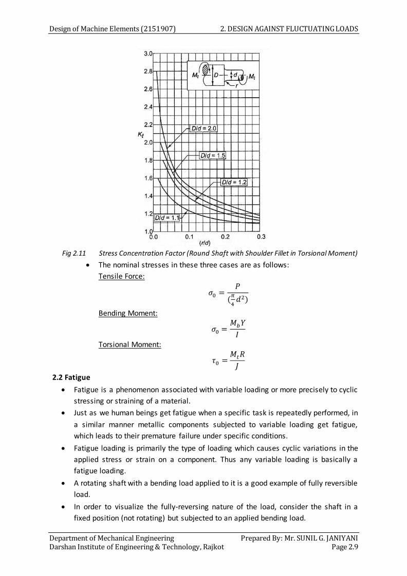
Design of Machine Elements (2151907) 2. DESIGN AGAINST FLUCTUATING LOADS
Department of Mechanical Engineering Prepared By: Mr. SUNIL G. JANIYANI Darshan Institute of Engineering & Technology, Rajkot Page 2.9
Fig 2.11 Stress Concentration Factor (Round Shaft with Shoulder Fillet in Torsional Moment)
The nominal stresses in these three cases are as follows:
Tensile Force:
Bending Moment:
Torsional Moment:
2.2 Fatigue
Fatigue is a phenomenon associated with variable loading or more precisely to cyclic
stressing or straining of a material.
Just as we human beings get fatigue when a specific task is repeatedly performed, in
a similar manner metallic components subjected to variable loading get fatigue,
which leads to their premature failure under specific conditions.
Fatigue loading is primarily the type of loading which causes cyclic variations in the
applied stress or strain on a component. Thus any variable loading is basically a
fatigue loading.
A rotating shaft with a bending load applied to it is a good example of fully reversible
load.
In order to visualize the fully-reversing nature of the load, consider the shaft in a
fixed position (not rotating) but subjected to an applied bending load.

2. DESIGN AGAINST FLUCTUATING LOADS Design of Machine Elements (2151907)
Prepared By: Mr. SUNIL G. JANIYANI Department of Mechanical Engineering Page 2.10 Darshan Institute of Engineering & Technology, Rajkot
The outermost fibers on the shaft surface lying on the convex side of the deflection
(upper surface) will be loaded in tension, and the fibers on the opposite side will be
loaded in compression.
Now, rotate the shaft 180° in its bearings, with the loads remaining the same. The
shaft stress level is the same, but now the fibers which were loaded in compression
before you rotated it are now loaded in tension, and vice-versa.
Thus if the shaft is rotated let us say at 900 revolutions per minute then the shaft is
cyclically stressed 900 times a minute.
2.2.1 Fatigue failure
Fatigue failure is defined as time delayed –fracture under cyclic loading.
Examples of parts in which fatigue failures are common: transmission shafts,
connecting rods, gears, vehicle suspension springs and ball bearings.
The materials fail under fluctuating stresses at a stress magnitude which is
lower than the ultimate tensile strength of the material.
It has been found that the magnitude of the stress causing fatigue failure
decreases as the number of stress cycles increase.
This phenomenon of decreased resistance of the materials to fluctuating
stresses is the main characteristic of fatigue failure.
Three stages are involved in fatigue failure:
1. Crack initiation
2. Crack propagation
3. Fracture
1. Crack initiation:
Areas of localized stress concentrations such as fillets, notches, key ways, bolt
holes and even scratches or tool marks are potential zones for crack
initiation.
Cracks also generally originate from a geometrical discontinuity.
2. Crack propagation:
This further increases the stress levels and the process continues,
propagating the cracks across the grains or along the grain boundaries, slowly
increasing the crack size.
As the size of the crack increases the cross sectional area resisting the applied
stress decreases and reaches a level at which it is insufficient to resist the
applied stress.
3. Final fracture:
As the area becomes too insufficient to resist the induced stresses any
further a sudden fracture results in the component.
Fatigue cracks are not visible till they reach the surface of the component and
by that time the failure have already taken place.
The fatigue failure is sudden and total.

Design of Machine Elements (2151907) 2. DESIGN AGAINST FLUCTUATING LOADS
Department of Mechanical Engineering Prepared By: Mr. SUNIL G. JANIYANI Darshan Institute of Engineering & Technology, Rajkot Page 2.11
The fatigue failure, however, depends upon a number of factors, such as the
number of cycles, mean stress, stress amplitude, stress concentration,
residual stresses, corrosion and creep.
This makes the design of components subjected to fluctuating stresses more
complex.
2.2.2 Cyclic Stresses
Cyclic stresses may be classified as below:
1. Fluctuating stresses
2. Repeated stresses
3. Reversed stresses
1. Fluctuating Stresses:
Fig 2.12 Fluctuating Stresses
In many applications, the components are subjected to forces, which are not
static, but vary in magnitude with respect to time.
The stresses induced due to such forces are called fluctuating stresses. These
fluctuating stresses result in fatigue failure.
It varies in sinusoidal manner with respect to time and fluctuates between
maximum and minimum value.
It has some mean value as well as some amplitude value.
2. Repeated Stresses:
It varies in sinusoidal manner with respect to time but the variation is from
zero to maximum value.
And therefore

2. DESIGN AGAINST FLUCTUATING LOADS Design of Machine Elements (2151907)
Prepared By: Mr. SUNIL G. JANIYANI Department of Mechanical Engineering Page 2.12 Darshan Institute of Engineering & Technology, Rajkot
Fig 2.13 Repeated Stresses
3. Reversed Stresses:
Fig 2.14 Reversed Stresses
It varies in sinusoidal manner with respect to time but it has zero mean value.
Half portion of the cycle consists of tensile stress and the remaining half of
compressive stress.
2.2.3 Endurance Limit
Fatigue or endurance limit of a material is defined as the maximum
amplitude of completely reversed stress that the standard specimen can
sustain for an unlimited number of cycles without fatigue failure.
Fig 2.15 Comparison of fatigue limit
Fatigue or endurance limit can also be defined as the magnitude of stress
amplitude value at or below which no fatigue failure will occur, no matter
how large the number of stress reversals are, in other words leading to an
infinite life to the component.

Design of Machine Elements (2151907) 2. DESIGN AGAINST FLUCTUATING LOADS
Department of Mechanical Engineering Prepared By: Mr. SUNIL G. JANIYANI Darshan Institute of Engineering & Technology, Rajkot Page 2.13
Since the fatigue test cannot be conducted for unlimited or infinite number
of cycles, 106 (10 million) cycles is considered as a sufficient number of cycles
to define the endurance limit.
Most non-ferrous metals have no endurance limit.
For such materials, which do not have an endurance limit, it is customary to
define fatigue strength.
Fatigue or endurance strength is the stress level that produces failure after a
specified number of cycles (usually 5 x 10⁶ or 107).
2.2.4 Fatigue life
Fig 2.16 Specimen for Fatigue Test
Fatigue life is defined as the number of stress cycles that the standard
specimen can complete during the test before the appearance of the first
fatigue crack.
This specimen is carefully machined and polished.
The dimensions of the standard test specimen are in mm as shown in Fig.
2.16.
In the laboratory, the endurance limit is determined by means of a rotating
beam machine developed by R. R. Moore.
Fig 2.17 Rotating Beam Fatigue Testing Machine
The principle of a rotating beam is illustrated in Fig. 2.17.
A beam of circular cross-section is subjected to bending moment Mb.
It is subjected to a completely reversed stress cycle.
Changing the bending moment by addition or deletion of weights can vary
the stress amplitude.

2. DESIGN AGAINST FLUCTUATING LOADS Design of Machine Elements (2151907)
Prepared By: Mr. SUNIL G. JANIYANI Department of Mechanical Engineering Page 2.14 Darshan Institute of Engineering & Technology, Rajkot
The specimen is rotated by an electric motor.
The number of revolutions before the appearance of the first fatigue crack is
recorded on a revolution counter.
In each test, two readings are taken, viz., stress amplitude (Sf) and number of
stress cycles (N).
These readings are used as two coordinates for plotting a point on the S-N
diagram.
This point is called failure point.
To determine the endurance limit of a material, a number of tests are to be
carried out.
2.2.5 S – N curve
Fig 2.18 S-N Curve for Steels
The S-N curve is the graphical representation of stress amplitude (Sf) versus
the number of stress cycles (N) before the fatigue failure on a log-log graph
paper.
The S-N curve for steels is illustrated in Fig. 2.18.
Each test on the fatigue testing machine gives one failure point on the S-N
diagram.
In practice, the points are scattered in the figure and an average curve is
drawn through them.
For ferrous materials like steels, the S-N curve becomes straight at 106 cycles,
which indicates the stress amplitude corresponding to infinite number of
stress cycles.
The magnitude of this stress amplitude at 106 cycles represents the
endurance limit of the material
The S-N curve shown in figure is valid only for ferrous metals.
For nonferrous metals like aluminum alloys, the S-N curve slopes gradually
even after 107 cycles.

Design of Machine Elements (2151907) 2. DESIGN AGAINST FLUCTUATING LOADS
Department of Mechanical Engineering Prepared By: Mr. SUNIL G. JANIYANI Darshan Institute of Engineering & Technology, Rajkot Page 2.15
2.2.6 Low-Cycle and High-Cycle Fatigue
Fig 2.19 Low-Cycle and High-Cycle Fatigue
The body of knowledge available on fatigue failure from N=1 to N=1000
cycles is generally classified as low-cycle fatigue.
High-cycle fatigue, then, is concerned with failure corresponding to stress
cycles greater than 1000 cycles.
2.2.7 Notch Sensitivity
It is observed that the actual reduction in the endurance limit of a material
due to stress concentration is less than the amount indicated by the
theoretical stress concentration factor Kt.
Kt is the theoretical stress concentration factor, which is applicable to ideal
materials that are homogeneous, isotropic and elastic.
Kf is the fatigue stress concentration factor. This factor Kf is applicable to
actual materials and depends upon the grain size of the material.
Notch sensitivity is defined as the susceptibility of a material to succumb (fail
to resist) to the damaging effects of stress raising notches in fatigue loading.
The notch sensitivity factor is denoted by q.
Since σ0 = nominal stress as obtained by elementary equations
Increase of actual stress over nominal stress = (Kf σ0 – σ0)
Increase of theoretical stress over nominal stress = (Kt σ0 – σ0)
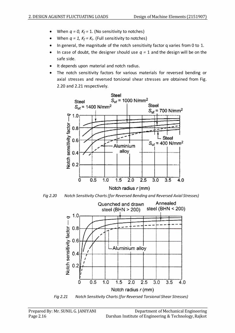
2. DESIGN AGAINST FLUCTUATING LOADS Design of Machine Elements (2151907)
Prepared By: Mr. SUNIL G. JANIYANI Department of Mechanical Engineering Page 2.16 Darshan Institute of Engineering & Technology, Rajkot
When q = 0, Kf = 1. (No sensitivity to notches)
When q = 1, Kf = Kt. (Full sensitivity to notches)
In general, the magnitude of the notch sensitivity factor q varies from 0 to 1.
In case of doubt, the designer should use q = 1 and the design will be on the
safe side.
It depends upon material and notch radius.
The notch sensitivity factors for various materials for reversed bending or
axial stresses and reversed torsional shear stresses are obtained from Fig.
2.20 and 2.21 respectively.
Fig 2.20 Notch Sensitivity Charts (for Reversed Bending and Reversed Axial Stresses)
Fig 2.21 Notch Sensitivity Charts (for Reversed Torsional Shear Stresses)

Design of Machine Elements (2151907) 2. DESIGN AGAINST FLUCTUATING LOADS
Department of Mechanical Engineering Prepared By: Mr. SUNIL G. JANIYANI Darshan Institute of Engineering & Technology, Rajkot Page 2.17
2.3 Factors Affecting Endurance Strength
The endurance strength (Se) of a component is different from the endurance
strength (Se’) of a rotating beam specimen due to number of factors.
The difference arises due to the fact that there are standard specifications and
working conditions for the rotating beam specimen, while the actual components
have different specifications and work under different conditions.
Different modifying factors are used in practice to account for this difference. These
factors are, sometimes, called “derating factors”.
The purpose of derating factors is to 'derate' or reduce the endurance limit of a
rotating beam specimen to suit the actual component.
The relationship between (Se’) and (Se) is as follows:
Se = Ka Kb Kc Kd Se’
where, Ka = Surface finish factor
Kb = Size factor
Kc = Reliability factor
Kd = Modifying factor to account for stress concentration
Se’ = Endurance limit stress of a rotating beam specimen subjected to
reversed bending stress (N/mm2)
Se = Endurance limit stress of a particular mechanical component subjected
to reversed bending stress (N/mm2)
Endurance limit:
There is an approximate relationship between the endurance limit and the
ultimate tensile strength (Sut) of the material.
For steels, Se’ = 0.5 Sut
For cast iron and cast steels, Se’ = 0.4 Sut
For wrought aluminum alloys, Se’ = 0.4 Sut
For cast aluminum alloys, Se’ = 0.3 Sut
Surface finish factor (Ka):
Fig 2.22 Surface finish factor

2. DESIGN AGAINST FLUCTUATING LOADS Design of Machine Elements (2151907)
Prepared By: Mr. SUNIL G. JANIYANI Department of Mechanical Engineering Page 2.18 Darshan Institute of Engineering & Technology, Rajkot
Rotating beam specimen is polished to mirror finish.
It is impractical to provide such an expensive surface finish for the actual
component. This poor surface finish increases stress concentration.
It depends upon ultimate tensile strength and process used to manufacture
the component.
It should be noted that ultimate tensile strength is also a parameter affecting
the surface finish factor.
High strength materials are more sensitive to stress concentration introduced
by surface irregularities. Therefore, as the ultimate tensile strength increases,
the surface finish factor decreases.
Size factor (Kb):
In rotating beam specimen, the diameter is small as 7.5 mm. Larger the
component, greater the probability of variation in size. Therefore, the
endurance limit reduces with increase in size of component.
For bending and Torsion, the values of size factor (Kb) are given in Table 2.1. Table 2.1 Values of Size Factor
Diameter (d) (mm) Kb d ≤ 7.5 1.00
7.5 < d ≤ 50 0.85 d > 50 0.75
Reliability factor (Kc):
There is considerable variation of the data when number of tests is
conducted even when using the same material.
The greater the likelihood that a part will survive, the more is the reliability
and lower is the reliability factor.
The reliability factor is one for 50% reliability. This means that 50% of the
components will survive in the given set of conditions.
To ensure that more than 50% of the parts will survive, the stress amplitude
on the component should be lower than the tabulated value of the
endurance limit.
The reliability factor is used to achieve this reduction.
The tests are considered to be 50 % reliable. Hence for 50% reliability, Kc = 1.
Table 2.2 Reliability Factor
Reliability (R) (%) Kc
50 1.000
90 0.897
95 0.868
99 0.814
99.9 0.753
99.99 0.702
99.999 0.659

Design of Machine Elements (2151907) 2. DESIGN AGAINST FLUCTUATING LOADS
Department of Mechanical Engineering Prepared By: Mr. SUNIL G. JANIYANI Darshan Institute of Engineering & Technology, Rajkot Page 2.19
Modifying factor to account for stress concentration (Kd):
Due to notch sensitivity, fatigue stress concentration factor is less than the
theoretical stress concentration factor.
To apply the effect of stress concentration, the designer can reduce the
endurance limit by Kd.
The modifying factor Kd to account for the effect of stress concentration is
defined as,
The above mentioned four factors are used to find out the endurance limit of the
actual component.
All the above factors are considered for reversed bending stresses only.
The endurance limit (Sse) of a component subjected to fluctuating torsional shear
stresses is obtained from the endurance limit in reversed bending (Se) using theories
of failures.
According to the maximum shear stress theory,
Sse = 0.5 Se
According to distortion – energy theory,
Sse = 0.577 Se
When the component is subjected to an axial fluctuating load, the conditions are
different.
In axial loading, the entire cross-section is uniformly stressed to the maximum value.
Therefore, endurance limit in axial loading is lower than the rotating beam test.
For axial loading,
(Se)a= 0.8 Se
2.4 Design for Reversed Stresses
There are two types of problems in fatigue design:
(i) Components subjected to completely reversed stresses, and
(ii) Components subjected to fluctuating stresses.
The mean stress is zero in case of completely reversed stresses .
The stress distribution consists of tensile stresses for the first half cycle and
compressive stresses for the remaining half cycle and the stress cycle passes through
zero.
In case of fluctuating stresses, there is always a mean stress, and the stresses can be
purely tensile, purely compressive or mixed depending upon the magnitude of the
mean stress. Such problems are solved with the help of the modified Goodman
diagram.
The design problems for completely reversed stresses are further divided into two
groups:
a) Design for infinite life, and
b) Design for finite life.
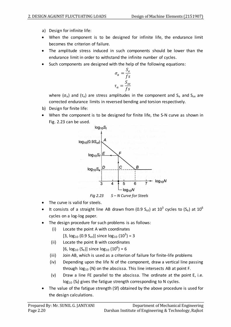
2. DESIGN AGAINST FLUCTUATING LOADS Design of Machine Elements (2151907)
Prepared By: Mr. SUNIL G. JANIYANI Department of Mechanical Engineering Page 2.20 Darshan Institute of Engineering & Technology, Rajkot
a) Design for infinite life:
When the component is to be designed for infinite life, the endurance limit
becomes the criterion of failure.
The amplitude stress induced in such components should be lower than the
endurance limit in order to withstand the infinite number of cycles.
Such components are designed with the help of the following equations:
where (σa) and (τa) are stress amplitudes in the component and Se and Sse are
corrected endurance limits in reversed bending and torsion respectively.
b) Design for finite life:
When the component is to be designed for finite life, the S-N curve as shown in
Fig. 2.23 can be used.
Fig 2.23 S – N Curve for Steels
The curve is valid for steels.
It consists of a straight line AB drawn from (0.9 Sut) at 103 cycles to (Se) at 106
cycles on a log-log paper.
The design procedure for such problems is as follows:
(i) Locate the point A with coordinates
[3, log10 (0.9 Sut)] since log10 (103) = 3
(ii) Locate the point B with coordinates
[6, log10 (Se)] since log10 (106) = 6
(iii) Join AB, which is used as a criterion of failure for finite-life problems
(iv) Depending upon the life N of the component, draw a vertical line passing
through log10 (N) on the abscissa. This line intersects AB at point F.
(v) Draw a line FE parallel to the abscissa. The ordinate at the point E, i.e.
log10 (Sf) gives the fatigue strength corresponding to N cycles.
The value of the fatigue strength (Sf) obtained by the above procedure is used for
the design calculations.

Design of Machine Elements (2151907) 2. DESIGN AGAINST FLUCTUATING LOADS
Department of Mechanical Engineering Prepared By: Mr. SUNIL G. JANIYANI Darshan Institute of Engineering & Technology, Rajkot Page 2.21
2.5 Design for Fluctuating Stresses
Fig 2.24 Gerber Line, Soderberg Line and Goodman Line
When stress amplitude (σa) is zero, the load is purely static and the criterion of
failure is Sut, or Syt.
When the mean stress (σm) is zero, the stress is completely reversing and the
criterion of failure is the endurance limit Se.
When the component is subjected to both components of stress, viz. (σ m) and
(σa), the actual failure occurs at different scattered points as shown in Fig. 2.24.
There exists a border, which divides safe region from unsafe region for various
combinations of (σm) and (σa).
Different criterions are proposed to construct the border line dividing safe zone
and failure zone.
They include Gerber line, Soderberg line and Goodman line.
(i) Gerber line:
A parabolic curve joining Se on the ordinate to Sut on the abscissa is called the
Gerber tine.
The Gerber parabola fits the failure points of test data in the best possible
way.
According to the Gerber line, the region below this curve is considered to be
safe.
Equation for the Gerber line is:
(
)
(ii) Soderberg line:
A straight line joining Se on the ordinate to Syt on the abscissa is called the
Soderberg line.

2. DESIGN AGAINST FLUCTUATING LOADS Design of Machine Elements (2151907)
Prepared By: Mr. SUNIL G. JANIYANI Department of Mechanical Engineering Page 2.22 Darshan Institute of Engineering & Technology, Rajkot
The Soderberg line is more conservative failure criterion and there is no need
to consider even yielding in this case.
Equation for the Soderberg line is:
(iii) Goodman line:
A straight line joining Se on the ordinate to Sut on the abscissa is called the
Goodman line.
Goodman line is safer from design considerations because it is completely
inside the Gerber parabola and inside the failure points.
Equation for the Goodman line is:
2.6 Modified Goodman Diagrams:
The components, which are subjected to fluctuating stresses, are designed by
constructing the modified Goodman diagram.
For the purpose of design, the problems are classified into two groups:
(i) Components subjected to fluctuating axial or bending stresses; and
(ii) Components subjected to fluctuating torsional shear stresses
(i) Modified Goodman Diagram for Axial and Bending Stresses :
Fig 2.25 Modified Goodman Diagram for Axial and Bending Stresses
The Goodman line is 'modified' by combining fatigue failure with failure by
yielding.
In this diagram, the yield strength Syt is plotted on both the axes and a yield
line CD is constructed to join these two points to define failure by yielding.
Obviously, the line CD is inclined at 45⁰ to the abscissa.

Design of Machine Elements (2151907) 2. DESIGN AGAINST FLUCTUATING LOADS
Department of Mechanical Engineering Prepared By: Mr. SUNIL G. JANIYANI Darshan Institute of Engineering & Technology, Rajkot Page 2.23
A line AF is constructed to join Se on the ordinate with Sut on the abscissa,
which is the Goodman line.
The point of intersection of these two lines is B.
The area OABC represents the region of safety for components subjected to
fluctuating stresses.
The region OABC is called modified Goodman diagram.
All the points inside the modified Goodman diagram should cause neither
fatigue failure nor yielding.
A line OE with a slope of “tan θ” is constructed in such a way that,
The magnitudes of (Mb)a and (Mb)m can be determined from maximum and
minimum bending moment acting on the component.
The point of intersection of lines AB and OE is X.
The point X indicates the dividing line between the safe region and the region
of failure.
The coordinates of the point X (Sm, Sa) represent the limiting values of
stresses, which are used to calculate the dimensions of the component.
The permissible stresses are as follows:
(ii) Modified Goodman Diagram for Torsional Shear Stresses:
Fig 2.26 Modified Goodman Diagram for Torsional Shear Stresses
In this diagram, the torsional mean stress is plotted on the abscissa while the
torsional stress amplitude on the ordinate.
The torsional yield strength Ssy is plotted on the abscissa and the yield line is
constructed, which is inclined at 45⁰ to the abscissa.
It is interesting to note that up to a certain point, the torsional mean stress
has no effect on the torsional endurance limit.

2. DESIGN AGAINST FLUCTUATING LOADS Design of Machine Elements (2151907)
Prepared By: Mr. SUNIL G. JANIYANI Department of Mechanical Engineering Page 2.24 Darshan Institute of Engineering & Technology, Rajkot
Therefore, a line is drawn through Sse on the ordinate and parallel to the
abscissa.
The point of intersection of this line and the yield line is B. The area OABC
represents the region of safety in this case.
It is not necessary to construct a fatigue diagram for fluctuating torsional
shear stresses because AB is parallel to the X-axis.
Instead, a fatigue failure is indicated if,
τa = Sse
The permissible stresses are as follows:
Example 2.1 A plate made of steel 20C8 (Sut = 440 N/mm2) in hot rolled and normalized
condition is shown in Fig. 2.27. It is subjected to a completely reversed load of 30 kN.
The notch sensitivity factor q can be taken as 0.8 and the expected reliability is 90%.
The size factor is 0.85. The factor of safety is 2. Determine the plate thickness for
infinite life. (V. B. Bhandari Example 5.3)
Fig 2.27 Given Figure for Example 2.1
Date Given:
Hot rolled steel
Ultimate tensile strength, Sut = 440 N/mm2
Load, P = 30 KN = 30000 N
Notch sensitivity factor, q = 0.8
Expected reliability, R = 90%
Size factor, Kb = 0.85
Factor of safety, fs = 2
Find thickness, “t”
Data from given figure:
Diameter of hole in the plate, d = 10 mm
Width of the plate, w = 50 mm

Design of Machine Elements (2151907) 2. DESIGN AGAINST FLUCTUATING LOADS
Department of Mechanical Engineering Prepared By: Mr. SUNIL G. JANIYANI Darshan Institute of Engineering & Technology, Rajkot Page 2.25
Solution:
From Fig. 2.22, for Hot rolled steel and Sut = 440 N/mm2, Surface finish factor, Ka = 0.67
From table 2.2, for R = 90%, Reliability factor, Kc = 0.897
From given figure, d = 10 mm and w = 50 mm,
From Fig. 2.7, for
, theoretical stress concentration factor, Kt = 2.51
Fatigue stress concentration factor,
Modifying factor to account for stress concentration,
For steels, Se’ = 0.5 Sut = 0.5 (440) = 220 N/mm2
Endurance limit stress of the component, Se = Ka Kb Kc Kd Se’
Se = 0.67 (0.85) (0.897) (0.4529) (220)
Se = 50.9 N/mm2
Permissible stress amplitude,
N/mm2
Example 2.2 A component machined from a plate made of steel 45C8 (Sut = 630 N/mm2)
is shown in Fig. 2.28. It is subjected to a completely reversed axial force of 50 kN. The
expected reliability is 90% and the factor of safety is 2. The size factor is 0.85.
Determine the plate thickness t for infinite life, if the notch sensitivity factor is 0.8.
(V. B. Bhandari Example 5.5)
Fig 2.28 Given Figure for Example 2.2

2. DESIGN AGAINST FLUCTUATING LOADS Design of Machine Elements (2151907)
Prepared By: Mr. SUNIL G. JANIYANI Department of Mechanical Engineering Page 2.26 Darshan Institute of Engineering & Technology, Rajkot
Date Given:
Machined steel, Ultimate tensile strength, Sut = 630 N/mm2
Load, P = 50 KN = 50000 N (Axial)
Expected reliability, R = 90%
Factor of safety, fs = 2
Size factor, Kb = 0.85
Notch sensitivity factor, q = 0.8
Find thickness, “t”
Data from given figure:
Larger width of the plate, D = 100 mm
Smaller width of the plate, d = 50 mm
Fillet radius at shoulder of the plate, r = 5 mm
Solution:
From Fig. 2.22, for machined steel and Sut = 630 N/mm2, Surface finish factor, Ka = 0.76
From table 2.2, for R = 90%, Reliability factor, Kc = 0.897
From given figure, D = 100 mm, d = 50 mm and r = 5 mm,
&
From Fig. 2.8, for
&
, theoretical stress concentration factor, Kt = 2.27
Fatigue stress concentration factor,
Modifying factor to account for stress concentration,
For steels, Se’ = 0.5 Sut = 0.5 (630) = 315 N/mm2
Endurance limit stress of the component, Se = Ka Kb Kc Kd Se’
Se = 0.76 (0.85) (0.897) (0.496) (315)
Se = 90.54 N/mm2
The load acting on the plate is axial and for axial loading,
(Se)a = 0.8 Se = 0.8(90.54) = 72.43 N/mm2
Permissible stress amplitude,
N/mm2

Design of Machine Elements (2151907) 2. DESIGN AGAINST FLUCTUATING LOADS
Department of Mechanical Engineering Prepared By: Mr. SUNIL G. JANIYANI Darshan Institute of Engineering & Technology, Rajkot Page 2.27
Example 2.3 A rotating bar made of steel 45C8 (Sut = 630 N/mm2) is subjected to a
completely reversed bending stress. The corrected endurance limit of the bar is 315
N/mm2. Calculate the fatigue strength of the bar for a life of 90,000 cycles.
(V. B. Bhandari Example 5.6)
Solution:
Date Given:
Ultimate tensile strength, Sut = 630 N/mm2
Endurance limit stress, Se = 315 N/mm2
Life of the bar, N = 90000 Cycles
Find fatigue strength, “Sf”
Solution:
Fig 2.29 S – N Diagram Drawn for Example 2.3
Refer Fig. 2.29, for solving this example following things are required.
Log Se = Log 315 = 2.4983
Log N = Log 90000 = 4.9542
Log (0.9 Sut) = Log (0.9 x 630) = 2.7536
From Fig. 2.29,
From Fig. 2.29,
Log Sf = Log (0.9 Sut) – AE
Log Sf = 2.7536 – 0.1663 = 2.5873
Sf = 386.63 N/mm2
Example 2.4 A forged steel bar, 50 mm in diameter, is subjected to a reversed bending
stress of 250 N/mm2. The bar is made of steel 40C8 (Sut = 600 N/mm2). Calculate the
life of the bar for a reliability of 90%. (V. B. Bhandari Example 5.7) (GTU Example)

2. DESIGN AGAINST FLUCTUATING LOADS Design of Machine Elements (2151907)
Prepared By: Mr. SUNIL G. JANIYANI Department of Mechanical Engineering Page 2.28 Darshan Institute of Engineering & Technology, Rajkot
Date Given:
Forged steel bar
Diameter of bar = 50 mm
Reversed bending stress or fatigue strength, Sf = 250 N/mm2
Ultimate tensile strength, Sut = 600 N/mm2
Expected reliability, R = 90%
Find life of bar, “N”
Solution:
From Fig. 2.22, for forged bar and Sut = 600 N/mm2, Surface finish factor, Ka = 0.44
From table 2.1, for d = 50 mm, Size factor, Kb = 0.85
From table 2.2, for R = 90%, Reliability factor, Kc = 0.897
For circular bar, effect of stress concentration will be negligible, hence modifying factor
to account for stress concentration,
For steels, Se’ = 0.5 Sut = 0.5 (600) = 300 N/mm2
Endurance limit stress of the component, Se = Ka Kb Kc Kd Se’
Se = 0.44 (0.85) (0.897) (1) (300)
Se = 100.64 N/mm2
Fig 2.30 S – N Diagram Drawn for Example 2.4
Refer Fig. 2.30, for solving this example following things are required.
Log Se = Log 100.64 = 2.0028
Log Sf = Log 250 = 2.3979
Log (0.9 Sut) = Log (0.9 x 600) = 2.7324
From Fig. 2.30,

Design of Machine Elements (2151907) 2. DESIGN AGAINST FLUCTUATING LOADS
Department of Mechanical Engineering Prepared By: Mr. SUNIL G. JANIYANI Darshan Institute of Engineering & Technology, Rajkot Page 2.29
From Fig. 2.30,
Log N = 3 + EF
Log N = 3 + 1.3574 = 4.3574
N = 23736 Cycles
Example 2.5 A rotating shaft subjected to a non-rotating force of 5 kN and simply
supported between two bearings A and E as shown in Fig. 2.31. The shaft is machined
from plain carbon steel 30C8 (Sut = 500 N/mm2) and the expected reliability is 90 %.
The equivalent notch radius at the fillet section can be taken as 3 mm. What is the life
of the shaft? Bending moment at section B is 642.9 kN.mm; surface finish factor =0.79;
size factor = 0.85; reliability factor = 0.897; stress concentration factor = 1.72; notch
sensitivity = 0.78. (V. B. Bhandari Example 5.8) (GTU Example)
Fig 2.31 Given Figure for Example 2.5
Date Given:
Material – Steel
Force, P = 5 KN = 5000 N
Ultimate tensile strength, Sut = 500 N/mm2
Expected reliability, R = 90%
Maximum bending moment, Mb = 642.9 kN mm = 642.9 x 10³ N mm
Surface finish factor, Ka = 0.79
Size factor, Kb = 0.85
Reliability factor, Kc = 0.897
Theoretical stress concentration factor, Kt = 1.72
Notch sensitivity factor, q = 0.78
Find life of the shaft, “N”
Data from given figure:
Smallest diameter of the shaft, d = 30 mm
Solution:
Fatigue stress concentration factor,

2. DESIGN AGAINST FLUCTUATING LOADS Design of Machine Elements (2151907)
Prepared By: Mr. SUNIL G. JANIYANI Department of Mechanical Engineering Page 2.30 Darshan Institute of Engineering & Technology, Rajkot
Modifying factor to account for stress concentration,
For steels, Se’ = 0.5 Sut = 0.5 (500) = 250 N/mm2
Endurance limit stress of the component, Se = Ka Kb Kc Kd Se’
Se = 0.79 (0.85) (0.897) (0.64) (250)
Se = 96.37 N/mm2
Maximum bending moment,
Here d = 30 mm because it is the weakest section of the shaft as it is having the smallest
diameter of the given shaft.
Here σb corresponds to fatigue strength, hence σb = Sf = 242.54 N/mm2
Fig 2.32 S – N Diagram Drawn for Example 2.5
Refer Fig. 2.32, for solving this example following things are required.
Log Se = Log 96.37 = 1.9839
Log Sf = Log 242.54 = 2.3848
Log (0.9 Sut) = Log (0.9 x 500) = 2.6532
From Fig. 2.32,

Design of Machine Elements (2151907) 2. DESIGN AGAINST FLUCTUATING LOADS
Department of Mechanical Engineering Prepared By: Mr. SUNIL G. JANIYANI Darshan Institute of Engineering & Technology, Rajkot Page 2.31
From Fig. 2.32,
Log N = 3 + EF
Log N = 3 + 1.203 = 4.203
N = 15960 Cycles
Example 2.6 A cantilever beam made of cold drawn steel 40C8 (Sut = 600 N/mm2 and Syt
= 380 N/mm2) is shown in Fig. 2.33. The force P acting at the free end varies from -50 N
to +150 N. The expected reliability is 90% and the factor of safety is 2. The notch
sensitivity factor at the fillet is 0.9. Determine the diameter d of the beam at the fillet
cross-section. (V. B. Bhandari Example 5.12)
Fig 2.33 Given Figure for Example 2.6
Date Given:
Cold drawn steel
Ultimate tensile strength, Sut = 600 N/mm2
Yield strength, Syt = 380 N/mm2
Maximum load, Pmax = +150 N
Minimum load, Pmin = -50 N
Expected reliability, R = 90%
Factor of safety, fs = 2
Notch sensitivity factor, q = 0.9
Find diameter, “d”
Data from given figure:
D = 1.5 d
r = 0.2 d
Solution:
From Fig. 2.22, for cold drawn steel and Sut = 600 N/mm2, Surface finish factor, Ka = 0.77
Assuming 7.5 < d < 50, hence from table 2.1, size factor, Kb = 0.85
From table 2.2, for R = 90%, Reliability factor, Kc = 0.897
From given figure,
&
From Fig. 2.10, for
&
, theoretical stress concentration factor, Kt = 1.44
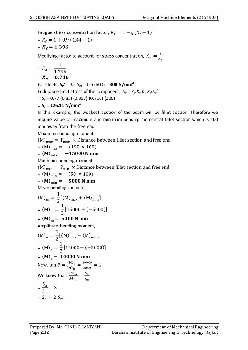
2. DESIGN AGAINST FLUCTUATING LOADS Design of Machine Elements (2151907)
Prepared By: Mr. SUNIL G. JANIYANI Department of Mechanical Engineering Page 2.32 Darshan Institute of Engineering & Technology, Rajkot
Fatigue stress concentration factor,
Modifying factor to account for stress concentration,
For steels, Se’ = 0.5 Sut = 0.5 (600) = 300 N/mm2
Endurance limit stress of the component, Se = Ka Kb Kc Kd Se’
Se = 0.77 (0.85) (0.897) (0.716) (300)
Se = 126.11 N/mm2
In this example, the weakest section of the beam will be fillet section. Therefore we
require value of maximum and minimum bending moment at fillet section which is 100
mm away from the free end.
Maximum bending moment,
Minimum bending moment,
Mean bending moment,
[ ]
[ ]
Amplitude bending moment,
[ ]
[ ]
Now,
We know that,

Design of Machine Elements (2151907) 2. DESIGN AGAINST FLUCTUATING LOADS
Department of Mechanical Engineering Prepared By: Mr. SUNIL G. JANIYANI Darshan Institute of Engineering & Technology, Rajkot Page 2.33
Fig 2.34 Modified Goodman Diagram Drawn for Example 2.6
Equation for the Goodman line is,
We know that,
We know that,
Permissible stress amplitude,
N/mm2
Amplitude bending moment,
Example 2.7 A cantilever beam made of cold drawn carbon steel of circular cross-section
as shown in Fig. 2.35, is subjected to a load which varies from – F to 3 F. Determine the
maximum load that the member can withstand for an indefinite life using a factor of
safety as 2. The theoretical stress concentration factor is 1.42 and the notch sensitivity
is 0.9. Assume the following values: Ultimate stress = 550 MPa, Yield stress = 470 MPa,
Endurance limit = 275 MPa, Size factor = 0.85, Surface finish factor= 0.89

2. DESIGN AGAINST FLUCTUATING LOADS Design of Machine Elements (2151907)
Prepared By: Mr. SUNIL G. JANIYANI Department of Mechanical Engineering Page 2.34 Darshan Institute of Engineering & Technology, Rajkot
(R. S. Khurmi Example 6.10) (GTU Example)
Fig 2.35 Given Figure for Example 2.7
Date Given:
Cold drawn, Carbon steel
Maximum load, Pmax = + 3 F
Minimum load, Pmin = - F
Factor of safety, fs = 2
Theoretical stress concentration factor, Kt = 1.42
Notch sensitivity factor, q = 0.9
Ultimate tensile strength, Sut = 550 N/mm2
Yield strength, Syt = 470 N/mm2
Endurance limit, Se’ = 275 N/mm2
Size factor, Kb = 0.85
Surface finish factor, Ka = 0.89
Find, “F”
Solution:
Reliability factor is not given hence assuming R = 50%, therefore from table 2.2, for R =
50%, Reliability factor, Kc = 1
Fatigue stress concentration factor,
Modifying factor to account for stress concentration,
Endurance limit stress of the component, Se = Ka Kb Kc Kd Se’
Se = 0.89 (0.85) (1) (0.7257) (275)
Se = 151 N/mm2
In this example, the weakest section of the beam will be fillet section. Therefore we
require value of maximum and minimum bending moment at fillet section which is 125
mm away from the free end.

Design of Machine Elements (2151907) 2. DESIGN AGAINST FLUCTUATING LOADS
Department of Mechanical Engineering Prepared By: Mr. SUNIL G. JANIYANI Darshan Institute of Engineering & Technology, Rajkot Page 2.35
Maximum bending moment,
Minimum bending moment,
Mean bending moment,
[ ]
[ ]
Amplitude bending moment,
[ ]
[ ]
Now,
We know that,
Equation for the Goodman line is,
We know that,
We know that,
Permissible stress amplitude,

2. DESIGN AGAINST FLUCTUATING LOADS Design of Machine Elements (2151907)
Prepared By: Mr. SUNIL G. JANIYANI Department of Mechanical Engineering Page 2.36 Darshan Institute of Engineering & Technology, Rajkot
N/mm2
Amplitude bending moment,
Here d = 13 mm because it is the weakest section of the shaft as it is having the smallest
diameter of the given shaft.
We know that,
Example 2.8 A transmission shaft of cold drawn steel 27Mn2 (Sut = 500 N/mm2 and Syt =
300 N/mm2) is subjected to a fluctuating torque which varies from - 100 N-m to + 400
N-m. The factor of safety is 2 and the expected reliability is 90%. Neglecting the effect
of stress concentration, determine the diameter of the shaft. Assume the distortion
energy theory of failure. (V. B. Bhandari Example 5.13) (GTU Example)
Date Given:
Cold drawn steel
Ultimate tensile strength, Sut = 500 N/mm2
Yield strength, Syt = 300 N/mm2
Maximum torque, Tmax = + 400 N m = + 400 x 103 N mm
Minimum torque, Tmin = - 100 N m = - 100 x 103 N mm
Factor of safety, fs = 2
Expected reliability, R = 90%
Neglect the effect of stress concentration
Find, diameter of shaft “d”
Assume the distortion energy theory of failure
Solution:
From Fig. 2.22, for cold drawn steel and Sut = 500 N/mm2, Surface finish factor, Ka = 0.79
Assuming 7.5 < d < 50, hence from table 2.1, size factor, Kb = 0.85
From table 2.2, for R = 90%, Reliability factor, Kc = 0.897
It is given that neglect the effect of stress concentration, hence modifying factor to
account for stress concentration, Kd = 1
For steels, Se’ = 0.5 Sut = 0.5 (500) = 250 N/mm2
Endurance limit stress of the component, Se = Ka Kb Kc Kd Se’
Se = 0.79 (0.85) (0.897) (1) (250)
Se = 150.58 N/mm2
It is given that assume the distortion energy theory of failure.

Design of Machine Elements (2151907) 2. DESIGN AGAINST FLUCTUATING LOADS
Department of Mechanical Engineering Prepared By: Mr. SUNIL G. JANIYANI Darshan Institute of Engineering & Technology, Rajkot Page 2.37
N/mm2
For fluctuating torque,
N/mm2
Permissible amplitude shear stress,
N/mm2
Amplitude torque,
[ ]
[ ]
Amplitude torque,
τ
τ
Example 2.9 A machine component is subjected to fluctuating stress that varies from 40
to 100 N/mm2. The corrected endurance limit stress for the machine component is 270
N/mm2. The ultimate tensile strength and yield strength of the material are 600 and
450 N/mm2 respectively. Find the factor of safety using:
(i) Gerber theory;
(ii) Soderberg line;
(iii) Goodman line; and
(iv) Static failure.
(V. B. Bhandari Example 5.17) (GTU Example)
Date Given:
Maximum stress, σmax = 100 N/mm2
Minimum stress, σmin = 40 N/mm2
Endurance limit, Se = 270 N/mm2
Ultimate tensile strength, Sut = 600 N/mm2
Yield strength, Syt = 450 N/mm2
Find factor of safety for different given criteria.
Solution:
N/mm2
N/mm2
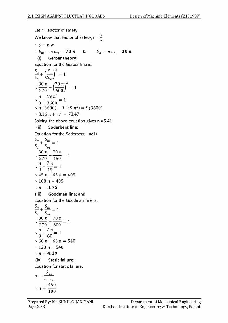
2. DESIGN AGAINST FLUCTUATING LOADS Design of Machine Elements (2151907)
Prepared By: Mr. SUNIL G. JANIYANI Department of Mechanical Engineering Page 2.38 Darshan Institute of Engineering & Technology, Rajkot
Let n = Factor of safety
We know that Factor of safety, n =
&
(i) Gerber theory:
Equation for the Gerber line is:
(
)
(
)
Solving the above equation gives n = 5.41
(ii) Soderberg line:
Equation for the Soderberg line is:
(iii) Goodman line; and
Equation for the Goodman line is:
(iv) Static failure:
Equation for static failure:

Design of Machine Elements (2151907) 2. DESIGN AGAINST FLUCTUATING LOADS
Department of Mechanical Engineering Prepared By: Mr. SUNIL G. JANIYANI Darshan Institute of Engineering & Technology, Rajkot Page 2.39
Example 2.10 A circular bar 500 mm length is supported freely at its two ends. It is acted
upon by a central concentrated cyclic load having a minimum value of 20 kN and a
maximum value of 50 kN. Determine the diameter of bar by taking factor of safety 1.5;
size effect of 0.85; surface finish factor of 0.9; The material properties of bars are given
by: ultimate strength of 650 MPa, yield strength of 500 MPa and endurance strength
of 350 MPa. (R. S. Khurmi Example 6.8) (GTU Example)
Date Given:
Length of bar, l = 500 mm (freely supported)
Maximum load, Pmax = 50 kN = 50000 N
Minimum load, Pmin = 20 kN = 20000 N
Factor of safety, fs = 1.5
Size factor, Kb = 0.85
Surface finish factor, Ka = 0.9
Ultimate tensile strength, Sut = 650 N/mm2
Yield strength, Syt = 500 N/mm2
Endurance strength, Se’ = 350 N/mm2
Find diameter, “d”
Solution:
Reliability factor is not given hence assuming R = 50%, therefore from table 2.2, for R =
50%, Reliability factor, Kc = 1
For circular bar, effect of stress concentration will be negligible, hence modifying factor
to account for stress concentration,
Endurance limit stress of the component, Se = Ka Kb Kc Kd Se’
Se = 0.9 (0.85) (1) (1) (350)
Se = 267.75 N/mm2
Maximum bending moment,
Minimum bending moment,
Mean bending moment,
[ ]
[ ]

2. DESIGN AGAINST FLUCTUATING LOADS Design of Machine Elements (2151907)
Prepared By: Mr. SUNIL G. JANIYANI Department of Mechanical Engineering Page 2.40 Darshan Institute of Engineering & Technology, Rajkot
Amplitude bending moment,
[ ]
[ ]
Now,
We know that,
Equation for the Goodman line is,
We know that,
We know that,
Permissible stress amplitude,
N/mm2
Amplitude bending moment,

Department of Mechanical Engineering Prepared By: Mr. SUNIL G. JANIYANI Darshan Institute of Engineering & Technology, Rajkot Page 3.1
3 DESIGN OF SPRINGS
Course Contents
3.1 Introduction to Spring
3.2 Types of springs
3.3 Spring Materials
3.4 Terminology of Helical
Springs
3.5 End Connections for
Compression Helical Springs
3.6 End Connections for Tension
Helical Springs
3.7 Buckling of Compression
Springs
3.8 Surge in Springs
3.9 Concentric or Composite
Springs
3.10 Springs in Series
3.11 Springs in Parallel
Examples

3. DESIGN OF SPRINGS Design of Machine Elements (2151907)
Prepared By: Mr. SUNIL G. JANIYANI Department of Mechanical Engineering Page 3.2 Darshan Institute of Engineering & Technology, Rajkot
3.1 Introduction to Spring
A spring is defined as an elastic machine element that deflects under the action of
the load and returns to its original shape when the load is removed.
It can take any shape and form depending upon the application.
Functions and applications of springs are listed in the below table.
Table 3.1 Functions and applications of springs
Function Applications
To absorb shocks
and vibrations
• Vehicle suspension springs
• Railway buffer springs
• Buffer springs in elevators
• Vibration mounts for machinery
To store energy • Springs used in clocks, toys. Movie-cameras, circuit
breakers and starters
To measure force • Springs used in weighing balance and engine indicators
To control Motion • In cam and follower mechanism, spring is used to
maintain contact between two elements.
To apply force • In engine valve mechanism, spring is used to return the
rocker arm to its normal position when the disturbing
force is removed.
• The spring used in clutch provides the required force to
engage the clutch.
3.2 Types of springs
Following are important types of springs according to their shape:
1. Helical springs
2. Conical and volute springs
3. Torsion springs
4. Laminated or leaf springs
5. Disc or belleville springs
3.2.1 Helical Springs
The helical spring is made from a wire, usually of circular cross section, that is
bent in the form of a helix.
There are two basic types of helical springs: compression spring and tension
spring.
In helical compression spring, the external force tends to shorten the spring.
In other words, the spring is compressed.
In helical tension spring, the external force tends to lengthen the spring. In
other words, the spring is elongated.

Design of Machine Elements (2151907) 3. DESIGN OF SPRINGS
Department of Mechanical Engineering Prepared By: Mr. SUNIL G. JANIYANI Darshan Institute of Engineering & Technology, Rajkot Page 3.3
Fig 3.1 (a) Compression Helical Spring (b) Tension Helical Spring
It should be noted that although the spring is under compression, the wire of
helical compression spring is not subjected to compressive stress.
Also, the wire of helical tension spring is not subjected to tensile stress
although the spring is under tension.
In both cases, torsional shear stresses are induced in the spring wire.
The words compression and tension are related to total spring and not the
stresses in spring wire.
3.2.2 Conical and Volute Springs
The conical and volute springs are used in special applications where a
telescoping spring or a spring with a spring rate (load required per unit
deflection) that increases with the load is desired.
The conical spring is wound with a uniform pitch whereas the volute springs
are wound in the form of paraboloid with constant pitch and lead angles.
This characteristic is sometimes utilised in vibration problems where springs
are used to support a body that has a varying mass.
Fig 3.2 (a) Conical spring (b) Volute spring

3. DESIGN OF SPRINGS Design of Machine Elements (2151907)
Prepared By: Mr. SUNIL G. JANIYANI Department of Mechanical Engineering Page 3.4 Darshan Institute of Engineering & Technology, Rajkot
Fig 3.3 Application of Conical and Volute Spring
3.2.3 Torsion Springs
The construction of this spring is similar to that of compression or tension
spring, except that the ends are formed in such away, that the spring is
loaded by a torque, about the axis of the coils.
Helical torsion spring is used to transmit torque to a particular component in
the machine or the mechanism.
Helical torsion spring is used in door-hinges, brush-holders, starters and door
locks.
Fig 3.4 Helical Torsion spring
For example, the spring transmits a torque of (P x r).
The helical torsion resists the bending moment (P x r) that tends to wind up
the spring.
The bending moment induces bending stresses in the spring wire.
The term torsion spring is somewhat misleading because wire is subjected to
bending stresses, unlike torsional shear stresses induced in helical torsion or
tension springs.

Design of Machine Elements (2151907) 3. DESIGN OF SPRINGS
Department of Mechanical Engineering Prepared By: Mr. SUNIL G. JANIYANI Darshan Institute of Engineering & Technology, Rajkot Page 3.5
Fig 3.5 Applications of Helical Torsion spring
3.2.4 Laminated Leaf Springs
Fig 3.6 Laminated Leaf Springs
Multi-leaf spring is widely used for the suspension of trucks and railway
wagons.
It consists of a series of flat plates, usually of semi-elliptical shape. The flat
plates are called leaves of the spring.
The leaf at the top has maximum length. The longest leaf at the top is called
master leaf.
The leaves have graduated lengths. The length gradually decreases from the
top leaf to the bottom leaf.
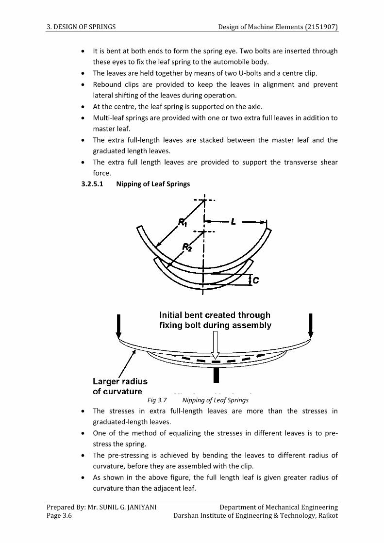
3. DESIGN OF SPRINGS Design of Machine Elements (2151907)
Prepared By: Mr. SUNIL G. JANIYANI Department of Mechanical Engineering Page 3.6 Darshan Institute of Engineering & Technology, Rajkot
It is bent at both ends to form the spring eye. Two bolts are inserted through
these eyes to fix the leaf spring to the automobile body.
The leaves are held together by means of two U-bolts and a centre clip.
Rebound clips are provided to keep the leaves in alignment and prevent
lateral shifting of the leaves during operation.
At the centre, the leaf spring is supported on the axle.
Multi-leaf springs are provided with one or two extra full leaves in addition to
master leaf.
The extra full-length leaves are stacked between the master leaf and the
graduated length leaves.
The extra full length leaves are provided to support the transverse shear
force.
3.2.5.1 Nipping of Leaf Springs
Fig 3.7 Nipping of Leaf Springs
The stresses in extra full-length leaves are more than the stresses in
graduated-length leaves.
One of the method of equalizing the stresses in different leaves is to pre-
stress the spring.
The pre-stressing is achieved by bending the leaves to different radius of
curvature, before they are assembled with the clip.
As shown in the above figure, the full length leaf is given greater radius of
curvature than the adjacent leaf.

Design of Machine Elements (2151907) 3. DESIGN OF SPRINGS
Department of Mechanical Engineering Prepared By: Mr. SUNIL G. JANIYANI Darshan Institute of Engineering & Technology, Rajkot Page 3.7
The radius of curvature decreases with shorter leaves.
The initial gap C between the extra full-length leaf and the graduated-length
leaf before the assembly is called a nip.
Such pre-stressing, achieved by a difference in radius of curvature, is known
as nipping.
3.2.5 Disc or belleville springs
Fig 3.8 Disc or Belleville springs
A Belleville spring consists of a coned disk, as shown in the above figure.
It is called Belleville spring because it was invented by Julian Belleville, who
patented its design in France in 1867.
Fig 3.9 Characteristic Curves for Disc or Belleville springs
Belleville spring has typical load deflection characteristic, as shown in the
above figure.

3. DESIGN OF SPRINGS Design of Machine Elements (2151907)
Prepared By: Mr. SUNIL G. JANIYANI Department of Mechanical Engineering Page 3.8 Darshan Institute of Engineering & Technology, Rajkot
The variation of (h/t) ratio provides a wide variety of load deflection curves.
Belleville springs are used in plate clutches and brakes, relief valves and a
wide variety of bolted connections.
(a) Series Combination (b) Parallel Combination (c) Parallel Series Combination
Fig 3.10 Disc or belleville springs
Belleville spring offers following advantages:
1. It is simple in construction and easy to manufacture.
2. It is a compact spring unit.
3. It is especially useful where very large force is desired for small
deflection of spring.
4. It provides a wide range of spring constants making it versatile.
5. It can provide any linear or non-linear load deflection characteristic.
6. The individual coned disks of a particular size and thickness can be
stacked in series, parallel or series parallel combinations, as shown in
Figure. These combinations provide a variety of spring constants
without changing the design.
7. When two Belleville springs are arranged in series, double deflection
is obtained for the same force. On the other hand, when two Belleville
springs are in parallel, almost double force is obtained for a given
deflection.
3.3 Spring Materials
The material of the spring should have high fatigue strength, high ductility, high
resilience and it should be creep resistant.
Selection of material for the spring wire depends upon following factors:
1. The load acting on the spring
2. The range of stress through which the spring operates
3. The limitations on mass and volume of spring
4. The expected fatigue life
5. The environmental conditions in which the spring will operate such as
temperature and corrosive atmosphere
6. The severity of deformation encountered while making the spring

Design of Machine Elements (2151907) 3. DESIGN OF SPRINGS
Department of Mechanical Engineering Prepared By: Mr. SUNIL G. JANIYANI Darshan Institute of Engineering & Technology, Rajkot Page 3.9
The mainly used material for manufacturing the springs are as follows:
1. Hard drawn high carbon steel
2. Oil tempered high carbon steel
3. Stainless steel
4. Copper or nickel based alloys
5. Phosphor bronze
6. Monel
7. Titanium
8. Chrome vanadium
9. Chrome silicon
Characteristics of some typical materials are explained below
1. Hard-drawn wire: This is cold drawn, cheapest spring steel. Normally used for
low stress and static load. The material is not suitable at subzero temperatures or
at temperatures above 120⁰ C.
2. Oil-tempered wire: It is a cold drawn, quenched, tempered, and general purpose
spring steel. However, it is not suitable for fatigue or sudden loads, at subzero
temperatures and at temperatures above 180⁰ C. When we go for highly stressed
conditions then alloy steels are useful.
3. Chrome Vanadium: This alloy spring steel is used for high stress conditions and at
high temperature up to 220⁰ C. It is good for fatigue resistance and long
endurance for shock and impact loads.
4. Chrome Silicon: This material can be used for highly stressed springs. It offers
excellent service for long life, shock loading and for temperature up to 250⁰ C.
5. Music wire: This spring material is most widely used for small springs. It is the
toughest and has highest tensile strength and can withstand repeated loading at
high stresses. However, it cannot be used at subzero temperatures or at
temperatures above 120⁰ C. Normally when we talk about springs we will find
that the music wire is a common choice for springs.
6. Stainless steel: Widely used alloy spring materials.
7. Phosphor Bronze / Spring Brass: It has good corrosion resistance and electrical
conductivity. That is the reason it is commonly used for contacts in electrical
switches. Spring brass can be used at subzero temperatures.
3.4 Terminology of Helical Springs
The main dimensions of a helical spring subjected compressive force are as follows:
d = wire diameter of spring
Di = inside diameter of spring coil
Do = outside diameter of spring coil
D = mean coil diameter
Therefore,

3. DESIGN OF SPRINGS Design of Machine Elements (2151907)
Prepared By: Mr. SUNIL G. JANIYANI Department of Mechanical Engineering Page 3.10 Darshan Institute of Engineering & Technology, Rajkot
Fig 3.11 Terminology of Helical Springs
1. Spring index (C): The spring index is defined as the ratio of mean coil diameter to
wire diameter. It is denoted by letter C.
The spring index indicates the relative sharpness of the curvature of the coil.
A low index means high sharpness of curvature.
When the spring index is low (C < 3), the actual stresses in the wire are
excessive due to curvature effect.
Such a spring is difficult to manufacture and special care in coiling is required
to avoid cracking in some wires.
When the spring index is high (C > 15), it results in large variation in coil
diameter.
Such a spring is prone to buckling and also tangles easily during handling.
Spring index from 4 to 12 is considered better from manufacturing
considerations. Therefore, in practical applications, the spring index usually
varies from 4 to 12.
However, the spring index in the range of 6 to 9 is still preferred particularly
for close tolerance springs and those subjected to cyclic loading.
Fig 3.12 Compression spring nomenclature

Design of Machine Elements (2151907) 3. DESIGN OF SPRINGS
Department of Mechanical Engineering Prepared By: Mr. SUNIL G. JANIYANI Darshan Institute of Engineering & Technology, Rajkot Page 3.11
2. Solid length: When the compression spring is compressed until the coils come in
contact with each other, then the spring is said to be solid.
The solid length of a spring is the product of total number of coils and the
diameter of the wire.
Mathematically, Solid length of the spring,
where n' = Total number of coils, and
d = Diameter of the wire.
3. Free length: The free length of a compression spring is the length of the spring in
the free or unloaded condition.
It is equal to the solid length plus the maximum deflection or compression of
the spring and the clearance between the adjacent coils (when fully
compressed).
Mathematically, Free length of the spring,
LF = Solid length + Maximum compression + Clearance between adjacent coils
4. Spring Rate: The spring rate (or stiffness or spring constant) is defined as the load
required per unit deflection of the spring.
Mathematically, Spring rate,
where W = Load, and
δ = Deflection of the spring
5. Pitch: It is defined as the axial distance between adjacent coils in uncompressed
state.
Mathematically,
6. A. M. Wahl’s Stress Factor and Curvature Effect:
Fig 3.13 Curvature Effect

3. DESIGN OF SPRINGS Design of Machine Elements (2151907)
Prepared By: Mr. SUNIL G. JANIYANI Department of Mechanical Engineering Page 3.12 Darshan Institute of Engineering & Technology, Rajkot
Let us look at a small section of a circular spring, as shown in the below figure.
Suppose we hold the section b-c fixed and give a rotation to the section a-d in
the anti-clockwise direction as indicated in the figure, then it is observed that
line a-d rotates and it takes up another position, say a'-d'.
The above phenomenon is termed as curvature effect.
So more is the spring index, the lesser will be the curvature effect.
In order to consider the effects of both direct shear as well as curvature of
the wire, a Wahl’s stress factor (K) introduced by A. M. Wahl may be used.
3.5 End Connections for Compression Helical Springs
(a)Plain ends (b) Ground ends (c) Squared ends (d) Squared & ground ends
Fig 3.14 End connections for compression helical spring
The end connections for compression helical springs are suitably formed in order to
apply the load. Various forms of end connections are shown in above figure.
In all springs, the end coils produce an eccentric application of the load, increasing
the stress on one side of the spring.
Under certain conditions, especially where the number of coils is small, this effect
must be taken into account.
The nearest approach to an axial load is secured by squared and ground ends, where
the end turns are squared and then ground perpendicular to the helix axis.
It may be noted that part of the coil which is in contact with the seat does not
contribute to spring action and hence are termed as inactive coils.
The turns which impart spring action are known as active turns.
As the load increases, the number of inactive coils also increases due to seating of
the end coils and the amount of increase varies from 0.5 to 1 turn at the usual
working loads.
The following table shows the total number of turns, solid length and free length for
different types of end connections.
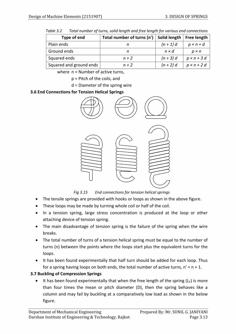
Design of Machine Elements (2151907) 3. DESIGN OF SPRINGS
Department of Mechanical Engineering Prepared By: Mr. SUNIL G. JANIYANI Darshan Institute of Engineering & Technology, Rajkot Page 3.13
Table 3.2 Total number of turns, solid length and free length for various end connections
Type of end Total number of turns (n') Solid length Free length
Plain ends n (n + 1) d p × n + d
Ground ends n n × d p × n
Squared ends n + 2 (n + 3) d p × n + 3 d
Squared and ground ends n + 2 (n + 2) d p × n + 2 d
where n = Number of active turns,
p = Pitch of the coils, and
d = Diameter of the spring wire
3.6 End Connections for Tension Helical Springs
Fig 3.15 End connections for tension helical springs
The tensile springs are provided with hooks or loops as shown in the above figure.
These loops may be made by turning whole coil or half of the coil.
In a tension spring, large stress concentration is produced at the loop or other
attaching device of tension spring.
The main disadvantage of tension spring is the failure of the spring when the wire
breaks.
The total number of turns of a tension helical spring must be equal to the number of
turns (n) between the points where the loops start plus the equivalent turns for the
loops.
It has been found experimentally that half turn should be added for each loop. Thus
for a spring having loops on both ends, the total number of active turns, n' = n + 1.
3.7 Buckling of Compression Springs
It has been found experimentally that when the free length of the spring (LF) is more
than four times the mean or pitch diameter (D), then the spring behaves like a
column and may fail by buckling at a comparatively low load as shown in the below
figure.

3. DESIGN OF SPRINGS Design of Machine Elements (2151907)
Prepared By: Mr. SUNIL G. JANIYANI Department of Mechanical Engineering Page 3.14 Darshan Institute of Engineering & Technology, Rajkot
Fig 3.16 Buckling of compression springs.
The critical axial load (Wcr) that causes buckling may be calculated by using the
following relation, i.e.
Wcr = k × KB × LF
where k = spring rate or stiffness of the spring = W/δ,
LF = Free length of the spring, and
KB = Buckling factor depending upon the ratio LF / D.
How to prevent buckling?
Free length (LF) should be less than 4 times the coil diameter (D) to avoid buckling.
Material should be selected having higher stiffness.
It order to avoid the buckling of spring, it is either mounted on a central rod or
located on a tube.
When the spring is located on a tube, the clearance between the tube walls and the
spring should be kept as small as possible, but it must be sufficient to allow for
increase in spring diameter during compression.
3.8 Surge in Springs
When one end of a helical spring is resting on a rigid support and the other end is
loaded suddenly, then all the coils of the spring will not suddenly deflect equally,
because some time is required for the propagation of stress along the spring wire.
A little consideration will show that in the beginning, the end coils of the spring in
contact with the applied load takes up whole of the deflection and then it transmits
a large part of its deflection to the adjacent coils.
In this way, a wave of compression propagates through the coils to the supported
end from where it is reflected back to the deflected end.
This phenomenon can also be observed in closed water body where a disturbance
moves toward the wall and then again returns back to the starting of the
disturbance.
This wave of compression travels along the spring indefinitely.

Design of Machine Elements (2151907) 3. DESIGN OF SPRINGS
Department of Mechanical Engineering Prepared By: Mr. SUNIL G. JANIYANI Darshan Institute of Engineering & Technology, Rajkot Page 3.15
If the applied load is of fluctuating type and if the time interval between the load
applications is equal to the time required for the wave to travel from one end to the
other end, then resonance will occur.
This results in very large deflections of the coils and correspondingly very high
stresses.
Under these conditions, it is just possible that the spring may fail. This phenomenon
is called surge.
How to prevent surging?
The surge in springs may be eliminated by using the following methods :
1. By using friction dampers on the centre coils so that the wave propagation dies
out.
2. By using springs of high natural frequency (the operational frequency of the
spring should be at least 15-20 times less than its fundamental frequency).
3. By using springs having pitch of the coils near the ends different than at the
centre to have different natural frequencies.
3.9 Concentric or Composite Springs
Fig 3.17 Concentric or Composite Springs
A concentric or composite or nested spring is used for one of the following purposes:
1. To obtain greater spring force within a given space.
2. To insure the operation of a mechanism in the event of failure of one of the
springs.

3. DESIGN OF SPRINGS Design of Machine Elements (2151907)
Prepared By: Mr. SUNIL G. JANIYANI Department of Mechanical Engineering Page 3.16 Darshan Institute of Engineering & Technology, Rajkot
The concentric springs for the above two purposes may have two or more springs
and have the same free lengths as shown in the above figure and are compressed
equally.
Such springs are used in automobile clutches; valve springs in aircraft, heavy duty
diesel engines and rail-road car suspension systems.
Let W = Axial load,
W1 = Load shared by outer spring,
W2 = Load shared by inner spring,
d1 = Diameter of spring wire of outer spring,
d2 = Diameter of spring wire of inner spring,
D1 = Mean diameter of outer spring,
D2 = Mean diameter of inner spring,
δ1 = Deflection of outer spring,
δ2 = Deflection of inner spring,
n1 = Number of active turns of outer spring,
n2 = Number of active turns of inner spring
We know that,
Also,
Equating the above both,
To consider effect of curvature of wire, a Wahl’s stress factor (K) is introduced in
case of helical spring.
where
Assuming that both the springs are made of same material, then the maximum shear
stress induced in both the springs is approximately same, i.e. τ1 = τ2.
( )
( )
When stress factor, K1 = K2,
( )
( )
( )

Design of Machine Elements (2151907) 3. DESIGN OF SPRINGS
Department of Mechanical Engineering Prepared By: Mr. SUNIL G. JANIYANI Darshan Institute of Engineering & Technology, Rajkot Page 3.17
Let l = Total active length of the wire
= Length of one coil x No. of active coils
= π D n
θ = Angular deflection of the wire when loaded
Therefore, Axial deflection of the spring,
( )
We know that,
Putting value of l, T and J in the above equation,
(
) ( )
(
)
( )( )
( )
Putting value θ in the equation (ii),
If both the springs are effective throughout their working range, then their free
length and deflection are equal, i.e., δ1 = δ2.
( )
( )
( )
( )
( )
( )
( )
( )
Multiply and divide by d1 & d2 on L.H.S. and R.H.S. respectively,
( )
( )
( )
( )
( )
( )
When both the springs are compressed until the adjacent coils meet, then the solid
length of both the springs is equal, i.e. n1 d1 = n2 d2.
The above equation may be written as,
( )
( )
( )
( )
( )

3. DESIGN OF SPRINGS Design of Machine Elements (2151907)
Prepared By: Mr. SUNIL G. JANIYANI Department of Mechanical Engineering Page 3.18 Darshan Institute of Engineering & Technology, Rajkot
Now dividing equation (iii) by equation (i), we have
( )
( )
( )
( )
( )
Therefore we can say that the spring index for both the springs is same.
From equations (iii) and (iv), we have
( )
( )
( )
( )
3.10 Springs in Series
Fig 3.18 Springs in Series
Consider two springs connected in series as shown in the figure above.
Let W = Load carried by the springs,
δ1 = Deflection of spring 1,
δ2 = Deflection of spring 2,
k1 = Stiffness of spring 1 = W / δ1
k2 = Stiffness of spring 2 = W / δ2
A little consideration will show that when the springs are connected in series, then
the total deflection produced by the springs is equal to the sum of the deflections of
the individual springs.
Hence total deflection of the springs,
δ = δ1 + δ2 ( )
We know that

Design of Machine Elements (2151907) 3. DESIGN OF SPRINGS
Department of Mechanical Engineering Prepared By: Mr. SUNIL G. JANIYANI Darshan Institute of Engineering & Technology, Rajkot Page 3.19
Putting value δ in the equation (v),
where k = Combined stiffness of springs
3.11 Springs in Parallel
Fig 3.19 Springs in Parallel
Consider two springs connected in parallel as shown in the above figure. Let W = Load carried by the springs, W
1 = Load shared by spring 1,
W2 = Load shared by spring 2,
k1 = Stiffness of spring 1
k2 = Stiffness of spring 2
A little consideration will show that when the springs are connected in parallel, then the total deflection produced by the springs is same as the deflection of the individual springs.
We know that W = W1 + W
2
Also
where k = Combined stiffness of the springs, and
δ = Deflection produced

3. DESIGN OF SPRINGS Design of Machine Elements (2151907)
Prepared By: Mr. SUNIL G. JANIYANI Department of Mechanical Engineering Page 3.20 Darshan Institute of Engineering & Technology, Rajkot
Table 3.3 Standard wire gauge (SWG) number and corresponding diameter of spring wire
SWG Diameter
(mm) SWG
Diameter (mm)
SWG Diameter
(mm) SWG
Diameter (mm)
7/0 12.7 7 4.47 20 0.914 33 0.254
6/0 11.785 8 4.064 21 0.813 34 0.2337
5/0 10.973 9 3.658 22 0.711 35 0.2134
4/0 10.16 10 3.251 23 0.61 36 0.193
3/0 9.49 11 2.946 24 0.559 37 0.1727
2/0 8.839 12 2.642 25 0.508 38 0.1524
0 8.229 13 2.337 26 0.457 39 0.1321
1 7.62 14 2.032 27 0.4166 40 0.1219
2 7.01 15 1.829 28 0.3759 41 0.1118
3 6.401 16 1.626 29 0.3454 42 0.1016
4 5.893 17 1.422 30 0.315 43 0.0914
5 5.385 18 1.219 31 0.2946 44 0.0813
6 4.877 19 1.016 32 0.2743 45 0.0711
Example 3.1 Design a helical compression spring for a maximum load of 1000 N for a
deflection of 25 mm using the value of spring index as 5. The maximum permissible
shear stress for spring wire is 420 MPa and modulus of rigidity is 84 kN / mm2.
(GTU Example)
Date Given:
W = 1000 N,
δ = 25 mm,
C = D/d = 5,
τ = 420 MPa = 420 N/mm2,
G = 84 kN/mm2 = 84 × 103 N/mm2
Solution:
Let D = Mean diameter of the spring coil, and
d = Diameter of the spring wire.
Wahl’s stress factor,
( )
( )
Maximum shear stress (τ),
( ) ( )

Design of Machine Elements (2151907) 3. DESIGN OF SPRINGS
Department of Mechanical Engineering Prepared By: Mr. SUNIL G. JANIYANI Darshan Institute of Engineering & Technology, Rajkot Page 3.21
From Table 3.3, we shall take a standard wire of size SWG 3 having diameter,
(d) = 6.401 mm.
Mean diameter of the spring coil,
D = C d = 5 d = 5 × 6.401 (where C = D/d)
D = 32.005 mm
Outer diameter of the spring coil,
Do = D + d = 32.005 + 6.401
Do = 38.406 mm
Inner diameter of the spring coil,
Di = D - d = 32.005 - 6.401
Di = 25.604 mm
Let n = Number of active turns of the coils
Deflection of the spring (δ),
( ) ( )
( ) ( )
For squared and ground ends, the total number of turns,
Free length of the spring (LF)
( ) ( )
Pitch of the coil (p),
Example 3.2 Design a close coiled helical compression spring for a service load ranging
from 2250 N to 2750 N. The axial deflection of the spring for the load range is 6 mm.
Assume a spring index of 5. The permissible shear stress intensity is 420 MPa and
modulus of rigidity, G = 84 kN/mm2. Neglect the effect of stress concentration.
(GTU Example)
Date Given:
W1 = 2250 N,

3. DESIGN OF SPRINGS Design of Machine Elements (2151907)
Prepared By: Mr. SUNIL G. JANIYANI Department of Mechanical Engineering Page 3.22 Darshan Institute of Engineering & Technology, Rajkot
W2 = 2750 N,
δ = 6 mm,
C = D/d = 5,
τ = 420 MPa = 420 N/mm2,
G = 84 kN/mm2 = 84 × 103 N/mm2
Solution:
Let D = Mean diameter of the spring coil for a maximum load of W2 = 2750 N, and
d = Diameter of the spring wire.
Twisting moment on the spring (T),
Also twisting moment on the spring (T),
( )
From Table 3.3, we shall take a standard wire of size SWG 3/0 having diameter,
(d) = 9.49 mm.
Mean diameter of the spring coil,
D = C d = 5 d = 5 × 9.49 (where C = D/d)
D = 47.45 mm
Outer diameter of the spring coil,
Do = D + d = 47.45 + 9.49
Do = 56.94 mm
Inner diameter of the spring coil,
Di = D - d = 47.45 - 9.49
Di = 37.96 mm
Let n = Number of active turns
It is given that the axial deflection (δ) for the load range from 2250 N to 2750 N (i.e. for
W = 500 N) is 6 mm.
Deflection of the spring (δ),
Design of Machine Elements (2151907) 3. DESIGN OF SPRINGS
Department of Mechanical Engineering Prepared By: Mr. SUNIL G. JANIYANI Darshan Institute of Engineering & Technology, Rajkot Page 3.23
( ) ( )
( ) ( )
For squared and ground ends, the total number of turns,
Since the deflection produced under 500 N is 6 mm, therefore maximum deflection
produced under the maximum load of 2750 N is
Free length of the spring (LF)
( ) ( )
Pitch of the coil (p),
Example 3.3 Design a helical spring for a spring loaded safety valve (Ramsbottom safety
valve) for the following conditions:
Diameter of valve seat = 65 mm,
Operating pressure = 0.7 N/mm2,
Maximum pressure when the valve blows off freely = 0.75 N/mm2,
Maximum lift of the valve when the pressure rises from 0.7 to 0.75 N/mm2 = 3.5 mm,
Maximum allowable stress = 550 MPa,
Modulus of rigidity = 84 kN/mm2,
Spring index = 6.
(GTU Example)
Date Given:
D1 = 65 mm,
p1 = 0.7 N/mm2,
p2 = 0.75 N/mm2,
δ = 3.5 mm,
τ = 550 MPa = 550 N/mm2,
G = 84 kN/mm2 = 84 × 103 N/mm2,
C = D/d = 6
Solution:

3. DESIGN OF SPRINGS Design of Machine Elements (2151907)
Prepared By: Mr. SUNIL G. JANIYANI Department of Mechanical Engineering Page 3.24 Darshan Institute of Engineering & Technology, Rajkot
Let D = Mean diameter of the spring coil, and
d = Diameter of the spring wire.
Since the safety valve is a Ramsbottom safety valve, therefore the spring will be under
tension.
We know that initial tensile force acting on the spring (i.e. before the valve lifts),
( )
( )
Maximum tensile force acting on the spring (i.e. when the valve blows off freely),
( )
( )
Force which produces the deflection of 3.5 mm,
Since the diameter of the spring wire is obtained for the maximum spring load (W2),
therefore maximum twisting moment on the spring,
Also twisting moment on the spring (T),
( )
From Table 3.3, we shall take a standard wire of size SWG 2/0 having diameter,
(d) = 8.839 mm.
Mean diameter of the spring coil,
D = C d = 6 d = 5 × 8.839 (where C = D/d)
D = 53.034 mm

Design of Machine Elements (2151907) 3. DESIGN OF SPRINGS
Department of Mechanical Engineering Prepared By: Mr. SUNIL G. JANIYANI Darshan Institute of Engineering & Technology, Rajkot Page 3.25
Outer diameter of the spring coil,
Do = D + d = 53.034 + 8.839
Do = 61.873 mm
Inner diameter of the spring coil,
Di = D - d = 53.034 - 8.839
Di = 44.195 mm
Let n = Number of active turns of the coils
Deflection of the spring (δ),
( ) ( )
( ) ( )
For a spring having loop on both ends, the total number of turns,
Taking the least gap between the adjacent coils as 1 mm when the spring is in free state,
the free length of the tension spring (LF),
( )
( ) ( )
Pitch of the coil (p),
Example 3.4 A rail wagon of mass 20 tones is moving with a velocity of 2 m/s. It is
brought to rest by two buffers with springs of 300 mm diameter. The maximum
deflection of springs is 250 mm. The allowable shear stress in the spring material is 600
MPa. Design the spring for the buffers.
(GTU Example)
Date Given:
m = 20 tones = 20000 kg,
v = 2 m/s,
D = 300 mm,
δ = 250 mm,
τ = 600 MPa = 600 N/mm2

3. DESIGN OF SPRINGS Design of Machine Elements (2151907)
Prepared By: Mr. SUNIL G. JANIYANI Department of Mechanical Engineering Page 3.26 Darshan Institute of Engineering & Technology, Rajkot
Solution:
Let d = Diameter of the spring wire
We know that kinetic energy of the wagon,
( )
( )
( )
Let W be the equivalent load which when applied gradually on each spring causes a
deflection of 250 mm.
Since there are two springs, energy stored in the springs,
( )
We know that the kinetic energy of the wagon is equal to the energy stored in the
springs. Hence equating (i) and (ii), we have
Twisting moment on the spring (T),
Also twisting moment on the spring (T),
( )
Outer diameter of the spring coil,
Do = D + d = 300 + 60
Do = 360 mm

Design of Machine Elements (2151907) 3. DESIGN OF SPRINGS
Department of Mechanical Engineering Prepared By: Mr. SUNIL G. JANIYANI Darshan Institute of Engineering & Technology, Rajkot Page 3.27
Inner diameter of the spring coil,
Di = D - d = 300 - 60
Di = 240 mm
Let n = Number of active turns of the coils
Deflection of the spring (δ),
(
)
( ) ( )
( ) ( )
For squared and ground ends, the total number of turns,
Free length of the spring (LF)
( ) ( )
Pitch of the coil (p),
Example 3.5 A semi-elliptic leaf spring used for automobile suspension consists of three
extra full –length leaves and 15 graduated-length leaves, including the master leaf. The
center-to-center distance between two eyes of the spring is 1 m. The maximum force
that can act on the spring is 75 KN. For each leaf, the ratio of width to thickness is 9:1.
The modulus of elasticity of the leaf material is 207000 N/mm2. The leaves are pre-
stressed in such a way that when the force is maximum, the stresses induced in all
leaves are same and equal to 450 N/mm2. Determine:
(i) The width and thickness of the leaves;
(ii) The initial nip; and
(iii) The initial pre-load required to close the gap C between extra full-length leaves
and graduated-length leaves.
(GTU Example)
Date Given:
2 P = 75 kN
P = 37.5 kN = 37500 N
2 L = 1 m

3. DESIGN OF SPRINGS Design of Machine Elements (2151907)
Prepared By: Mr. SUNIL G. JANIYANI Department of Mechanical Engineering Page 3.28 Darshan Institute of Engineering & Technology, Rajkot
L = 0.5 m = 500 mm
b = 9 t
nf = 3,
ng = 15,
E = 207000 N/mm2,
σb = 450 N/mm2
Solution:
Total number of leaves (n),
We know that,
( )( )
( )
( )( )
( ) ( )
It is given that,
( )
Initial nip (C),
( ) ( )
( ) ( ) ( )
Initial pre-load required (Pi)
( )
( )( ) ( )
* ( ) ( )+
Example 3.6 A semi-elliptic multi-leaf spring is used for the suspension of the rear axle of
a truck. It consists of two extra full length leaves and ten graduated length leaves
including the master leaf. The center to center distance between the two eyes of the
spring is 1.2 m and the width of the leaf is 60 mm. The leaves are made of steel
55Si2Mo90 (Syt = 1500 N/mm2 and E = 207000 N/mm2) and the factor of safety is 2.5.

Design of Machine Elements (2151907) 3. DESIGN OF SPRINGS
Department of Mechanical Engineering Prepared By: Mr. SUNIL G. JANIYANI Darshan Institute of Engineering & Technology, Rajkot Page 3.29
The spring is to be designed for a maximum force of 30 kN. The leaves are pre-stressed
so as to equalize stresses in all the leaves. Determine:
(i) The thickness of the leaves; and
(ii) The deflection at the end of the spring.
(GTU Example)
Date Given:
2 P = 30 kN
P = 15 kN = 15000 N
2 L = 1.2 m
L = 0.6 m = 600 mm
b = 60 mm
nf = 2,
ng = 10,
E = 207000 N/mm2,
Syt = 1500 N/mm2,
fs = 2.5
Solution:
Total number of leaves (n),
We know that,
( )( )
( )
( )( )
( ) ( )
Deflection of the spring (δ),
( )
( ) ( )
( ) ( ) * ( ) ( )+

Department of Mechanical Engineering Prepared By: Vimal G. Limbasiya Darshan Institute of Engineering & Technology, Rajkot Page 4.1
4 BELT AND CHAIN DRIVES
Course Contents
4.1 Introduction
4.2 Selection of Belt drive
4.3 Types of Belt drives
4.4 Types of Flat Belt drives
4.5 Law of Belting
4.6 Velocity Ratio of Belt drive
4.7 Creep of Belt
4.8 Length of an Open Belt drive
4.9 Length of Crossed Belt drive
4.10 Ratio of Friction Tensions
4.11 Power Transmitted by a belt
4.12 Angle of Contact or Angle of
Lap
4.13 Centrifugal effect on Belt
4.14 Maximum power transmitted
by a Belt
4.15 Initial Tension in the Belt
4.16 Advantages & Disadvantages
of V- Belt drive over Flat
Belt drive
4.17 Design of Pulleys
4.18 Design of Chain Drive

4. Belt and Chain Drives Design of Machine Elements (2151907)
Prepared By: Vimal G. Limbasiya Department of Mechanical Engineering Page 4.2 Darshan Institute of Engineering & Technology, Rajkot
4.1 Introduction Power is transmitted from one shaft to another by means of Belt, rope, chain and gears.
Salient Features:
1. Belt, rope and chain are used where the distance between the shaft is large. For small
distance gears are preferred.
2. Belt, rope and chain are flexible type of connectors, i.e., they are bent easily.
3. The flexibility of belt and rope is due to property of their materials whereas chains have a
number of small rigid elements having relative motion between the two elements.
4. Belt and rope transmit power due to friction between them and the pulley. If the power
transmitted exceeds the force of friction, the belt or rope slips over the pulley.
5. Belts and ropes are strained during motion as tensions are developed in them.
6. Owing to slipping and straining action belts and ropes are not positive drive, i.e., velocity
ratio are not constant. Chain and gears have constant velocity ratio.
4.2 Selection of Belt drive Speed of driving and driven shafts.
Power to be transmitted.
Space available.
Service conditions.
Centre distance between the shafts.
Speed reduction ratio.
4.3 Types of Belt drives 1. Light drives:-
Small power.
V ≤ 10 m/s Agricultural machine, Small machine.
2. Medium drives
Medium power
22 < V > 10 m/s, Machine tool.
3. Heavy drives
Large power
V > 22 m/s Compressor, generator.
Belt drives& its materials:
Fig. 4.1 Types of Belts

Design of Machine Elements (2151907) 4. Belt and Chain Drives
Department of Mechanical Engineering Prepared By: Vimal G. Limbasiya Darshan Institute of Engineering & Technology, Rajkot Page 4.3
1. Flat Belt:
Used in industry where moderate amount of power is transmitted.
Dist. x ≤ 8m or 10m apart with 22 m/sec.
Materials are leather, rubber, canvas, cotton & rubber Balata (higher strength than
rubber belt).
2. V- Belt:
Used in industry where moderate amount of power to be transmitted.
Connect the shaft up to 4m.
Speed ratio can be up to 7 to 1 and belt speed 24 m/sec.
Made of rubber impregnated fabric with angle of V between 30° to 40°.
Note: In mutiple V – belt drive all the belt should be stratch at the same rate so that load is
equally divided. When one of the self of belt break, the entire set should be replaced at the
same drive. If one belt is replaced the new unwarn and unstressed will be moretightly
stretched and will more with different velocity.
4.4 Types of Flat Belt Drives:
1. Open Belt Drive
Fig. 4.2 Open belt drive
An open belt drive is used when the driven pulley is desired rotate in the same direction.
Generally the centre distance for open belt drive is 14 – 16 m. if the distance is too large,
the belt whips i.e. vibrates in a direction perpendicular to the direction of motion.
For very shorter distance, the belt slips increase.
While transmitting power, one side of the belt is more tightened (known as tight side) as
compared to other (known as slack side).
In case of horizontal drives, it is always desired that the tight side is at the lower side of
two pulleys. This is because the sag of the belt will be more on the upper side than the
lower side. This is slightly increase the angle of wrap of the belts on the two pulleys than
if the belt had been perfectly straight between the pulleys.

4. Belt and Chain Drives Design of Machine Elements (2151907)
Prepared By: Vimal G. Limbasiya Department of Mechanical Engineering Page 4.4 Darshan Institute of Engineering & Technology, Rajkot
In case the tight side is on the upper side, the sag will be greater at the lower side,
reducing the angle of wrap and slip could occur earlier. This ultimately affects the power
to be transmitted.
2. Crossed Belt Drive
Fig. 4.3 Crossed belt drive
A crossed belt drive is used when the driven pulley is to be rotated in the opposite
direction to that of the driving pulley. A crossed belt drive can transmit more power than an open belt drive as the angle of
wrap is more. However the belt has to bend in two different planes and it wears out more. To avoid this
the shaft should be placed at a max dist. 20 b where b = width of belt and speed should
be less than 15 m /sec.
3. Quarter Turn Belt Drive / Right Angle Belt Drive
A guide pulley is used to connect two non-parallel shaft in such a way that they may run
in either direction, and still making the pulley to deliver the belt properly in accordance
with the law of belting.
Fig. 4.4 Quarter turn belt drive with guide pulley
A guide pulley can also be used to connect even intersecting shaft also.

Design of Machine Elements (2151907) 4. Belt and Chain Drives
Department of Mechanical Engineering Prepared By: Vimal G. Limbasiya Darshan Institute of Engineering & Technology, Rajkot Page 4.5
4. Belt Drive with Idler Pulley
Fig. 4.5 Belt drive with Idler pulley
With constant use the belt is permanently stretched in a little length. This reduces the
initial tension in the belt leading to lower power transmission capacity. However the
tension in the belt can be restored to the original value by using an arrangement shown
in figure.
A bell – crank lever, hinged on the axis of the smaller pulley, supports adjustable weights
on its one arm and the axis of a pulley on the other. The pulley is free to rotate on tis axis
and is known as idler pulley. Owing to weights on one arm of the lever, the pulley exerts
pressure on the belt increasing the tension and the angle of contact. Thus, life of the belt
is increased and the power capacity is restore to original value.
Motion of one shaft can be transmitted to two or more than two shafts by using a
number of idler pulley (figure).
5. Compound Belt Drive / Intermediate Pulley
Fig. 4.6 Compound belt drive
When it is required to have large velocity ratios, ordinarily the size of the larger pulley will
be quite big. However, by using an intermediate (counter shaft) pulley, the size can be
reduced.

4. Belt and Chain Drives Design of Machine Elements (2151907)
Prepared By: Vimal G. Limbasiya Department of Mechanical Engineering Page 4.6 Darshan Institute of Engineering & Technology, Rajkot
6. Stepped / Cone Pulley Drive
Fig. 4.7 Stepped / Cone pulley drive
A stepped cone pulley drive is used for changing the speed of the driven shaft while the
main or driving shaft runs at constant speed. This is done by shifting the belt from one part of the step to the other.
7. Fast and Loose Pulley drive
Many times, it is required to drive several machines from a single main shaft. In such a
case, some arrangement to link or delink a machine to or from the main shaft has to be
incorporated as all the machines may not be operating simultaneously. The arrangement
usually provides that of using a loose pulley along with a fast pulley.
Fig. 4.8 Fast and loose pulley drive
A fast pulley is keyed to the shaft and rotates with it at the same speed and thus
transmits power. A loose pulley is not keyed to the shaft and thus is unable to transmit any power.

Design of Machine Elements (2151907) 4. Belt and Chain Drives
Department of Mechanical Engineering Prepared By: Vimal G. Limbasiya Darshan Institute of Engineering & Technology, Rajkot Page 4.7
Whenever, a machine is to be driven, the belt is mounted on the fast pulley and when it
is not required to transmit any power, the belt is pushed to the loose pulley placed
adjacent to the fast pulley.
4.5 Law of Belting The law of belting states that centre line of the belt when it approaches a pulley must lie
in the mid plane of that pulley. However, a belt leaving a pulley may be drawn out of the
plane of the pulley.
By following this law, non – parallel shafts may be connected by a flat belt.
It should be observed that it is not possible to operate the belt in the reverse direction
without violating the law of belting. Thus, in case of non – parallel shafts, motion is
possible only in one direction. Otherwise, the belt is thrown off the pulley. However, it is
possible to run a belt in either direction on the pulley of two non – parallel or intersecting
shafts with the help of guide pulleys. The law of belting is satisfied.
4.6 Velocity Ratio of Belt Drive Velocity ratio is the ratio of speed of driven pulley (N2) to that of driving pulley (N1)
Let
N1 = Speed of driving pulley
N2 = Speed of driven pulley
D1 = Diameter of driving pulley
D2 = Diameter of the driven pulley
T = thickness of belt
Neglecting slip between belt & pulley and consider belt to be inelastic.
Let speed of belt on driving pulley = speed of belt on driven pulley
π D1 N1
60= π
D2 N2
60
D1 + 2 t
2 N1 = D2 + 2
t
2 N2
Or Velocity Ratio (VR)
VR = N2
N1=
D1 + t
D2 + t
Velocity Ratio of Compound Belt Drive
Let D1, D2,D3,D4 = Diameter of pulley
N1, N2,N3,N4 = Speed of pulley
For pulley 1 & 2 N2
N1=
D1
D2 _____________(1)

4. Belt and Chain Drives Design of Machine Elements (2151907)
Prepared By: Vimal G. Limbasiya Department of Mechanical Engineering Page 4.8 Darshan Institute of Engineering & Technology, Rajkot
For pulley 3 & 4 N4
N3=
D3
D4 _____________(2)
Multiplying (1) & (2) N2
N1 ×
N4
N3 =
D1
D2 ×
D3
D4
𝐍𝟒𝐍𝟏
= 𝐃𝟏𝐃𝟐
× 𝐃𝟑𝐃𝟒
4.7 Creep of Belt
When the belt passes from slack side to tight side, a certain portion of the belt extends
and it contracts again when the belt passes from tight side to slack side. Due to these
change of length, there is a relative motion between belt & pulley surface. This relative
motion is called “Creep”.
The total effect of creep is to reduce slightly the speed of the driven pulley or follower.
Considering the creep…….
Velocity ratio N2
N1=
d1
d2 E + σ2
E + σ1
Where
σ1 = Stress on the tight side of belt
σ2 = Stress on the slack side of belt
E = Young modulus for the belt material
4.8 Length of Open Belt Drive
Fig. 4.9 Length of an open belt drive
Let r1 , r2 = Radius of larger & smaller pulley.
x = Distance between centre of two pulley.
L = Total Length.
Let length of the belt,

Design of Machine Elements (2151907) 4. Belt and Chain Drives
Department of Mechanical Engineering Prepared By: Vimal G. Limbasiya Darshan Institute of Engineering & Technology, Rajkot Page 4.9
L = Arc GJE + EF + Arc FKH + GH
= 2 (Arc JE + EF + Arc FK)_____________(1)
Let
Arc EJG = 2 Arc JE = 2 π
2 + α ∙ r1
Arc FKH = 2 Arc FK = 2 π
2 − α ∙ r2
sinα = r1 − r2
x
EF = MO2 = O1O2 2 − O1M 2
= x 2 − r1 − r2 2
= x 1 − r1 − r2
𝑥
2
Expanding by Binominal Theorem
= x 1 − 1
2
r1 − r2
𝑥
2
+⋯⋯⋯ = x − 1
2
r1 − r2
x
2
Putting value in equation (1)
∴ L = 2 π
2 + α r1 + x −
r1 − r2 2
2x+
π
2 − α r2
= 2 r1 ∙π
2 + r1 ∙ α + x−
r1 − r2 2
2x+ r2 ∙
π
2 − r2 ∙ α
= 2 π
2 r1 + r2 + α r1 − r2 + x −
r1 − r2 2
2x
= π r1 + r2 + 2 α r1 − r2 + 2x − r1 − r2
2
x
sinα =
r1 − r2
xα is small∴ sin α = α

4. Belt and Chain Drives Design of Machine Elements (2151907)
Prepared By: Vimal G. Limbasiya Department of Mechanical Engineering Page 4.10 Darshan Institute of Engineering & Technology, Rajkot
= π r1 + r2 + 2 r1 − r2
𝑥 r1 − r2 + 2x −
r1 − r2 2
x
= π r1 + r2 + 2 r1 − r2
2
x+ 2x −
r1 − r2 2
x
L = π r1 + r2 + 2x + r1 − r2
2
x In terms of Radius
𝐋 = 𝛑
𝟐 𝐝𝟏 + 𝐝𝟐 + 𝟐𝐱 +
𝐝𝟏 − 𝐝𝟐 𝟐
𝟒𝐱 𝐈𝐧 𝐭𝐞𝐫𝐦𝐬 𝐨𝐟 𝐝𝐢𝐚𝐦𝐞𝐭𝐞𝐫
4.9 Length of Crossed Belt Drive
Fig. 4.10 Length of crossed belt drive
Let r1 , r2 = Radius of larger & smaller pulley.
x = Distance between centre of two pulley.
L = Total Length.
L = Arc GJE + Arc FKH + EF + GH _________(1)
Arc GJE = 2 Arc JE = 2 π
2 + α ∙ r1 _________(a)
Arc FKH = 2 Arc HK = 2 π
2 + α ∙ r2 _______(b)
EF = GH = MO2 = O1O2 2 − O2M 2
= 𝑥2 − r1 + r2 2
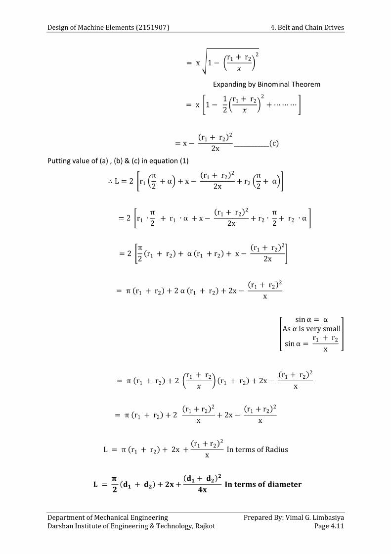
Design of Machine Elements (2151907) 4. Belt and Chain Drives
Department of Mechanical Engineering Prepared By: Vimal G. Limbasiya Darshan Institute of Engineering & Technology, Rajkot Page 4.11
= x 1 − r1 + r2
𝑥
2
Expanding by Binominal Theorem
= x 1 − 1
2
r1 + r2
𝑥
2
+⋯⋯⋯
= x − r1 + r2
2
2x____________(c)
Putting value of (a) , (b) & (c) in equation (1)
∴ L = 2 r1 π
2 + α + x −
r1 + r2 2
2x+ r2
π
2+ α
= 2 r1 ∙π
2 + r1 ∙ α + x−
r1 + r2 2
2x+ r2 ∙
π
2+ r2 ∙ α
= 2 π
2 r1 + r2 + α r1 + r2 + x −
r1 + r2 2
2x
= π r1 + r2 + 2 α r1 + r2 + 2x − r1 + r2
2
x
sinα = αAs α is very small
sinα = r1 + r2
x
= π r1 + r2 + 2 r1 + r2
𝑥 r1 + r2 + 2x −
r1 + r2 2
x
= π r1 + r2 + 2 r1 + r2
2
x+ 2x −
r1 + r2 2
x
L = π r1 + r2 + 2x + r1 + r2
2
x In terms of Radius
𝐋 = 𝛑
𝟐 𝐝𝟏 + 𝐝𝟐 + 𝟐𝐱+
𝐝𝟏 + 𝐝𝟐 𝟐
𝟒𝐱 𝐈𝐧 𝐭𝐞𝐫𝐦𝐬 𝐨𝐟 𝐝𝐢𝐚𝐦𝐞𝐭𝐞𝐫

4. Belt and Chain Drives Design of Machine Elements (2151907)
Prepared By: Vimal G. Limbasiya Department of Mechanical Engineering Page 4.12 Darshan Institute of Engineering & Technology, Rajkot
4.10 Ratio of Friction Tensions
1. Flat Belt
Fig. 4.11 Ratio of Friction Tensions for Flat Belt
T1 = Tensions on tight side.
T2 = Tensions on slack side.
θ = Angle of Lap of belt over pulley.
μ= Co – efficient of friction between belt & pulley.
Consider a short length of belt PQ subtending an angle of δθ at the centre of pulley.
R = Normal (Radial) reaction between element length of belt & pulley.
T = Tension on slack side of the element.
δT = increase in tension on tight side than that of slack side.
T + δT = Tension on tight side of element.
Tensions T and T + δT act in directions perpendicular to the radii drawn at the end of
elements. The friction force F = μR will act tangentially to the pulley rim resisting the
slipping of the elementary belt on the pulley.
Resolving the forces in tangential direction (Horizontally….),
μR + T cosδθ
2− T + δT cos
δθ
2= 0
μR + T − T + δT = 0
As δθ is small
cosδθ
2 ≈ 1
R = δT
μ _________(1)
Resolving the forces in Radial Direction (Vertically….),
R − T sinδθ
2− T + δT sin
δθ
2= 0
R − T δθ
2− T
δθ
2− δT ∙ δθ
2 = 0

Design of Machine Elements (2151907) 4. Belt and Chain Drives
Department of Mechanical Engineering Prepared By: Vimal G. Limbasiya Darshan Institute of Engineering & Technology, Rajkot Page 4.13
As δθ is small
sinδθ
2 ≈
δθ
2δT ∙ δθ
2 → Neglect
R = 2 Tδθ
2= T δθ _____(2)
Compare equation (1) and (2)
δT
μ= T δθ
∴δT
T= μ δθ
Integrating between proper limits…….
δT
T
T1
T2
= μ δθ
θ
0
∴ loge
T1
T2= μθ
Or taking a log to the base 10
𝐓𝟏𝐓𝟐
= 𝐞𝛍𝛉 2.3 logT1
T2= μθ
Note: The above relation is valid only when the belt is on the point of slipping on the
pulleys.
2. V – Belt
Fig. 4.12 Ratio of Friction Tensions for V-Belt
In case of v belt or rope, there are two normal reactions, so radial reaction is equal to
2R sinα
Thus total friction force = 2F = 2μR
Resolving the forces tangentially…….

4. Belt and Chain Drives Design of Machine Elements (2151907)
Prepared By: Vimal G. Limbasiya Department of Mechanical Engineering Page 4.14 Darshan Institute of Engineering & Technology, Rajkot
2μR + T cosδθ
2− T + δT cos
δθ
2= 0
2μR + T − T− δT = 0
As δθ is small
cosδθ
2 ≈ 1
δT = 2μR _________(1)
Resolving the forces radially……
2R sinα − T sinδθ
2− T + δT sin
δθ
2= 0
2R sinα − T δθ
2− T
δθ
2− δT ∙ δθ
2 = 0
As δθ is small
sinδθ
2 ≈
δθ
2δT ∙ δθ
2 → Neglect
2R sinα = 2 Tδθ
2
∴ R =Tδθ
2 sinα _____(2)
From equation (1) & (2)
δT = 2 μ Tδθ
2 sinα or
δT
T =
μ δθ
sinα
Integrating between proper limits
δT
T
T1
T2
= μ δθ
sinα
θ
0
∴ loge
T1
T2=
μθ
sinα
𝐓𝟏𝐓𝟐
= 𝐞𝛍𝛉 sin α
Note:-
The expression is similar to that for a flat belt drive except that μ is replaced by μ sin θ ,
i.e., the coefficient of friction is increased by 1 sin θ . Thus, the ratio T1 T2 is far greater
in case of V – belts & ropes for same angle of lapθ and coefficient of frictionμ.
Above expression is derived on the assumption that the belt is on the point of slipping.

Design of Machine Elements (2151907) 4. Belt and Chain Drives
Department of Mechanical Engineering Prepared By: Vimal G. Limbasiya Darshan Institute of Engineering & Technology, Rajkot Page 4.15
4.11 Power Transmitted by a belt
Let
T1 = Tensions on tight side.
T2 = Tensions on slack side.
V = Linear velocity of belt
P = Power transmitted
P = Net Force × Distance moved
second
= T1 − T2 V
Note:-This relation gives the power transmitted irrespective of the fact whether the belt is
on the point of slipping or not.
If it is the relationship between T1 and T2 for a flat belt is given by T1 T2 = eμθ . If it is not,
no particular relation is available to calculate T1 and T2.
4.12 Angle of Contact or Angle of Lap
1. Open Belt Drive
r1 = Radius of larger pulley.
r2 = Radius of smaller pulley.
x = Centre distance between two
pulley.
Angle of contact θ
θ = 180 − 2α °
= 180 − 2α π
180 Radian
Where sinα = r1 − r2
x
Fig. 4.13 Open belt drive
2. Cross Belt Drive
Angle of contact θ
θ = 180 + 2α °
= 180 + 2α π
180 Radian
Where sinα = r1 + r2
x
Fig. 4.14 Crossed Belt drive

4. Belt and Chain Drives Design of Machine Elements (2151907)
Prepared By: Vimal G. Limbasiya Department of Mechanical Engineering Page 4.16 Darshan Institute of Engineering & Technology, Rajkot
4.13 Centrifugal effect on Belt
Fig. 4.15 Centrifugal effect on Belt
While in motion, as a belt passes over a pulley, the centrifugal effect due to its own
weight tends to lift the belt from the pulley.
The centrifugal force produces equal tensions on the two side of belt, i.e., on the tight
and on the slack side.
Let
m = mass of belt per meter length (Kg/m).
v = Linear velocity of belt (m/sec).
r = Radius of pulley.
TC = Centrifugal tension on tight side & Slack side.
FC = Centrifugal force.
FC = mass of element × Acceleration
= Length of element × mass per unit length × Acc.
= r δθ × m ×v2
r ______(1)
From figure resolving forces radially…..
FC = 2 TC sinδθ
2
= 2 TC
δθ
2
δθ
2 is small
sinδθ
2 ≈
δθ
2
FC = TCδθ _______(2)
From Equation (1) & (2)
TCδθ = m v2δθ
∴ 𝐓𝐂 = 𝐦 𝐯𝟐

Design of Machine Elements (2151907) 4. Belt and Chain Drives
Department of Mechanical Engineering Prepared By: Vimal G. Limbasiya Darshan Institute of Engineering & Technology, Rajkot Page 4.17
∴ To depends only velocity of belt and mass of belt.
Also centrifugal stress in belt = centrifugal Tension
c s Area of belt=
TC
A
Or
TC = σ ∙ A (Max tension in belt)
Total Tension on tight side = Friction tension + Centrifugal tension
T = T1 + TC
Total Tension on slack side = T2 + TC
4.14 Maximum Power transmitted by a belt If it is desired that belt transmit maximum power, following two conditions must be
satisfied.
1. Larger tension must reach the maximum permissible value for the belt.
2. The belt should be on the point of slipping i.e., maximum frictional force is developed
in the belt.
Let
P = T1 − T2 ∙ v
= T1 1 − T2
T1 ∙ v
= T1 1− 1
T1
T2 ∙ v
T1
T2= eμθ
1 − 1
eμθ= k constant
= T1 k ∙ v
= T− TC ∙ k ∙ v
T = T1 + TC
∴ T1 = T − TC
= kTv− TC ∙ kv
= kTv− m v2 ∙ kv

4. Belt and Chain Drives Design of Machine Elements (2151907)
Prepared By: Vimal G. Limbasiya Department of Mechanical Engineering Page 4.18 Darshan Institute of Engineering & Technology, Rajkot
P = kTv− kmv3
Here maximum tension T in the belt should not exceed permissible value. Hence treating T
as constant and differentiating the power with respect to v and equating the same equal to
zero.
∴ dP
dv= kT − 3 v2 k m = 0
∴ kT = 3 v2 k m
T = 3 mv2
T = 3 TC or 𝐓𝐂 = 𝐓
𝟑
For maximum power transmission, the centrifugal tension in the belt is equal to 1/3 of
the maximum allowable belt tension and belt should be on the point of slipping.
Also T = T1 + TC
∴ T1 = T − TC
= T− T
3=
2T
3
Also T = 3TC
= 3 ∙m v2
∴ Vmax = T
3m
4.15 Initial Tension in the Belt
When a belt is first fitted to a pair of pulley, an initial tension T0 is given to the belt when
the system is stationary. When transmitting power, the tension on tight increases to T1
and that on slack side decreases to T2. If it is assumed that the material of the belt is perfectly elastic i.e., the strain in the belt is
proportional to stress in it and the total length of the belt remains unchanged, the
tension on the tight side will increase by the same amount as the tension on the slack
side decreases. If the change in the tension is δT…….
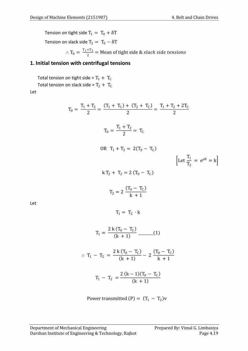
Design of Machine Elements (2151907) 4. Belt and Chain Drives
Department of Mechanical Engineering Prepared By: Vimal G. Limbasiya Darshan Institute of Engineering & Technology, Rajkot Page 4.19
Tension on tight side T1 = T0 + δT
Tension on slack side T2 = T0 − δT
∴ T0 = T1+T2
2= Mean of tight side & 𝑠𝑙𝑎𝑐𝑘 𝑠𝑖𝑑𝑒 𝑡𝑒𝑛𝑠𝑖𝑜𝑛𝑠
1. Initial tension with centrifugal tensions
Total tension on tight side = T1 + TC
Total tension on slack side = T2 + TC
Let
T0 = T1 + T2
2= T1 + TC + T2 + TC
2=
T1 + T2 + 2TC
2
T0 = T1 + T2
2= TC
OR T1 + T2 = 2 T0 − TC
Let T1
T2 = eμθ = k
k T2 + T2 = 2 T0 − TC
T2 = 2 T0 − TC
k + 1
Let
T1 = T2 ∙ k
T1 = 2 k T0 − TC
k + 1 ________(1)
∴ T1 − T2 = 2 k T0 − TC
k + 1 − 2
T0 − TC
k + 1
T1 − T2 =2 k− 1 T0 − TC
k + 1
Power transmitted P = T1 − T2 v

4. Belt and Chain Drives Design of Machine Elements (2151907)
Prepared By: Vimal G. Limbasiya Department of Mechanical Engineering Page 4.20 Darshan Institute of Engineering & Technology, Rajkot
= 2 k− 1 T0 − TC
k + 1 ∙ v
= 2 k− 1 T0 − m v2
k + 1∙ v
P = 2 k − 1 T0v− m v3
k + 1
To find the condition for maximum power transmission……
dP
dv= T0 − 3mv2 = 0
∴ T0 = 3mv2
∴ v = T0
3m
When the belt drive is started, v = 0 and thus TC = 0 TC = mv2
T1 = 2 k T0
k + 1 _________(2)
4.16 Advantages & Disadvantages of V – Belt drive over Flat Belt
drive
Advantages
1. V - Belt drive gives compactness due to small distance.
2. Drive is positive, because slip is less.
3. V – Belts are made endless, no joint so smooth drive.
4. Longer life 3 – 5 year.
5. Easily installed & removed.
6. High velocity ratio may be obtained.
7. Power transmission is more due to wedging action of the belt in groove.
8. V – Belt may be operated in either direction.
Disadvantages
1. V – Belt drive can’t use for large distance. 2. V – Beltsare not so durable as flat belts. 3. Construction of pulley for V – Belt is more complicated than the pulleys for flat belt.

Design of Machine Elements (2151907) 4. Belt and Chain Drives
Department of Mechanical Engineering Prepared By: Vimal G. Limbasiya Darshan Institute of Engineering & Technology, Rajkot Page 4.21
4. Since V – Belts are subjected to certain amount of creep, so they are not suitable for
constant speed application such as synchronous machines, timing devices etc. 5. Belt life is effect with temperature changes, improper belt tension and mismatching of
belt length. 6. The centrifugal tension prevents the use of V – Belts at speed below 5 m/s and above 50
m/sec.
4.17 Design of Pulleys
4.17.1 Pulleys for Flat Belts
The pulleys for flat belts consist of three parts, viz. rim, hub and arms or web. The rim
carries the belt. The hub connects the pulley to the shaft. T arms or web join the hub with
the rim. There are two types of pulleys that are used for flat belts viz., cast iron pulleys and
mild steel pulleys. The pulley diameters are calculated in belt drive design. They should
comply with standard values. The minimum pulley diameter depends upon the following
two factors:
(i) The number of plies in the belt
(ii) The belt speed
There is a specific term, 'crowning' of pulley in flat belt drive. The thickness of the rim is
slightly increased in the centre to give it a convex or conical shape as shown in Fig. 4.16. This
is called 'crown' of the pulley. The crown is provided only on one of the two pulleys. The
objectives of providing crown are as follows:
(i) The crown on the pulley helps to hold the belt on the pulley in running condition.
(ii) The crown on the pulley prevents the belt from running off the Pulley.
(iii) The crown on the pulley brings the belt to running equilibrium position near the
mid-plane of the Pulley.
Fig. 4.16 Crown for Pulley
The crown on pulley is essential, particularly when the pulleys are mounted inaccurately or
there is a possibility of slip due to non-parallelism between connected shafts.

4. Belt and Chain Drives Design of Machine Elements (2151907)
Prepared By: Vimal G. Limbasiya Department of Mechanical Engineering Page 4.22 Darshan Institute of Engineering & Technology, Rajkot
Fig. 4.17 Cast Iron Pulley
Cast iron pulleys are made of grey cast iron of Grade FG 200.
Mild steel pulleys are made of structural steels.
The rim and the arms or web are made of low carbon steel while the hub which is
subjected to crushing stress at the keyway, is made of medium carbon steel. The rim
is roll-formed from a steel plate and joined either by bolts or welded.
The arms are made of round steel bar and welded to the rim. The arms are welded
to the hub, if it is made of steel. The arms are screwed to the hub, if it is made of
cast iron. Mild steel pulleys have light weight construction compared with cast iron
pulleys.
4.17.2 V-Grooved Pulley
Fig. 4.18 Dimensions of V-grooved pulley
The dimensions of V–grooved pulley for V–belts are show in Fig. 4.18.
Such pulleys are usually made of grey cast iron of Grade–FG 250. In some
applications, the pulleys are made of carbon steel casting.

Design of Machine Elements (2151907) 4. Belt and Chain Drives
Department of Mechanical Engineering Prepared By: Vimal G. Limbasiya Darshan Institute of Engineering & Technology, Rajkot Page 4.23
The notations used in the Fig. 4.18. are as follows:
lp = Pitch width of pulley groove or pitch width of belt. It is the width of the belt at its
neutral axis. The line in the V-belt, whose length remains unchanged when the belt is
deformed under tension, is called its neutral axis.
b = Minimum height of groove above the pitch line
h = Minimum depth of groove below the pitch line
e = Centre to centre distance of adjacent grooves.
f = Distance of the edge of pulley to first groove center
α = Groove angle
dp = Pitch diameter of pulley. It is diameter of the pulley measured at the pitch width
of the groove
g = Minimum top width of the groove.
Arms of Cast Iron Pulley
There are three important things about the arms of the pulley. They are as follows:
(i) The arms of pulley have elliptical cross-section.
(ii) The major axis of elliptical cross-section is in the plane of rotation.
(iii) The major axis of elliptical cross-section is usually twice the minor axis.
Elliptical cross-section reduces aerodynamic losses during the rotation of pulley as
compared with rectangular cross-section. Therefore in variably, the arms have elliptical
cross-section.
The design of these arms illustrates the application of simple formula for bending stresses. It
is assumed that the belt wraps around the rim of the pulley through approximately 180 and
one-half of the arms carry the load at any moment. This is illustrated in Fig. 4.19.
Fig. 4.19
The torque transmitted by the pulley is given by,
t
nM PR
2 or, t2M
PRn
……………(a)
Where, Mt= torque transmitted by the pulley (N-mm)
P = tangential force at the end of each arm (N)

4. Belt and Chain Drives Design of Machine Elements (2151907)
Prepared By: Vimal G. Limbasiya Department of Mechanical Engineering Page 4.24 Darshan Institute of Engineering & Technology, Rajkot
R = radius of the rim (mm)
n = number of arms
As shown in Fig. 4.20, the bending moment acting on the arm is given by,
Mb = PR ……………(b)
From Eq. (a) and (b)
tb
2MM
n ...………….(c)
Fig. 4.20 Correct (Major axis is in plane of rotation)
The major axis of the elliptical cross-section is in the plane of rotation. For this elliptical
cross-section with a and b as minor and major axes respectively.
3I ab
64 …………...(d)
Since the major axis is twice of the minor axis,
b = 2a ………..….(e)
Substituting (e) and (d),
4I a
8 and
by a
2
The bending stress in the arm is given by,
b tb 4
M y (2M / n)(a)
I ( a / 8)
3 t
b
16 Ma
n
t3
b
Ma 1.72
n
…………….(f)
Where σb is the permissible bending stress.
Fig. 4.21 Incorrect (Minor axis is in plane of rotation)
If we consider the minor axis in the plane of rotation as illustrated in Fig. 4.21

Design of Machine Elements (2151907) 4. Belt and Chain Drives
Department of Mechanical Engineering Prepared By: Vimal G. Limbasiya Darshan Institute of Engineering & Technology, Rajkot Page 4.25
3I ba
64
Since the major axis is twice of the minor axis,
b = 2a
4I a
32 and
ay
2
The bending stress in the arm is given by,
b tb 4
M y (2M / n)(a/ 2)
I ( a / 32)
3 t
b
32 Ma
n
t3
b
Ma 2.17
n
……………(g)
It is observed from Eqs (f) and (g) that keeping the minor axis in the plane of rotation
increases the cross-sectional area. It is therefore 'economical' to keep major axis of elliptical
cross-section in the plane of rotation.
Design of pulley
Centrifugal stress induced in rim, σt = ρV2
ρ = Density of rim material
V = Velocity DN
60
Width of pulley, B is 25 % higher than width of belt
B = 1.25 b
Thickness of pulley rim
D
t 3200
for single belt
Dt 6
200 for double belt
Dimensions of arms
No. of arm, n = 4 for pulley diameter 200 to 600 mm
No. of arm, n = 6 for pulley diameter 600 to 1500 mm
Dimensions of hub
Diameter of hub, d1 = 1.5 d + 25 mm
Length of hub, 1L d2
d = diameter of shaft
Minimum length of hub = 2/3 B
Not more than width of pulley = B

4. Belt and Chain Drives Design of Machine Elements (2151907)
Prepared By: Vimal G. Limbasiya Department of Mechanical Engineering Page 4.26 Darshan Institute of Engineering & Technology, Rajkot
Example – 1:- Two parallel shafts connected by a crossed belt, are provided with pulleys
480 mm and 640 mm in diameters. The distance between the centre line of the shaft is 3 m.
Find by how much the length of the belt should be changed if it is desired to alter the
direction of rotation of the driven shaft.
Solution:
R = 320 mm
r = 240 mm
X = C = 3 mtr.
For cross belt drive
180 2180
For cross belt drive
cross
R r 320 240 0.320 0.240sin
C 3 3L 2 R r 2C Cos
10.75 10 45'0.1878 rad
crossL 2 0.1878 0.32 0.24 2 3 cos 10.757.865mtr.
For open belt drive
open 1 2 1 2
2
open
2
L r r 2 r r 2x cos
R rL R r 2C
C
0.32 0.240.32 0.24 2 3
37.761mtr.
1 2r rsin
X0.320 0.240
3
1 31'
Angle is small approx.
relation canbe used.
Let length of belt reduced by
cross oL L 7.865 7.761
0.104 mtr.
Example – 2:- A belt runs over a pulley of 800 mm diameter at a speed of 180 rpm. The
angle of lap is 165° and the maximum tension in the belt is 2kN. Determine the power
transmitted if the co – efficient of friction is 0.3.
Solution:

Design of Machine Elements (2151907) 4. Belt and Chain Drives
Department of Mechanical Engineering Prepared By: Vimal G. Limbasiya Darshan Institute of Engineering & Technology, Rajkot Page 4.27
1T 2000 Nd 0.8 mtr.N 180 rpm
165 rad180
2.88 rad
0.3
Let
0.8 180dN
V 7.54 m / sec60 60
110
2
T2.3log
T
110
2
T2.3log 0.3 2.88
T
1
2
T2.37
T
1
12
T 2000 NT 2000
T 843N2.37 2.37
1 2Power T T v
2000 843 7.54
8724 W
P 8.724 kW
Example – 3:- A casting weights 6 kN and is freely suspended from a rope which makes
2.5 turns round a drum of 200 mm diameter. If the drum rotates at 40 rpm, determine the
force required by a man to pull the rope form the other end of the rope. Also find the power
to raise the casting. The coefficient of friction is 0.25.
Solution:
1
2
W T 6000 N2.5 2 15.70 rad
d 0.20 mtr.N 40 rpm
0.25T ?P ?
Let
0.2 40dN
V 0.419 m / sec60 60

4. Belt and Chain Drives Design of Machine Elements (2151907)
Prepared By: Vimal G. Limbasiya Department of Mechanical Engineering Page 4.28 Darshan Institute of Engineering & Technology, Rajkot
110
2
T2.3log 0.25 15.70
T
12
2
T50.87 T 117.93N
T
1 2Power T T v
6000 117.93 0.419
2464 WattP 2.46 kW
Example – 4:- A belt drive transmits 8 kW of power from a shaft rotating at 240 rpm to
another shaft rotating at 160 rpm. The belt is 8 mm thick. The diameter of smaller pulley is
600 mm and the two shafts are 5 m apart. The coefficient of friction is 0.25. If the maximum
stress in the belt is limited to 3 N/mm2. Find the width of the belt for (i) open belt drive and
(ii) crossed belt drive.
Solution: 3
1 1
2
2
P 8 10 wattN 240 rpm , d 0.600 m (Smaller pulley)N 160 rpmx 5m
0.25t 8 mm
3N / mm
1 1 2 2N d N d
1 1
2
2
N d 240 0.6d 0.900 mtr. (bigger pulley)
N 160
(1) Open Belt drive
Angle of contact 180 2180
180 2 1.71180
3.08 rad
1 2r r 0.450 0.300sin
X 51.71
Let
110
2
T2.3log 0.25 3.08
T
1
2
T2.16
T

Design of Machine Elements (2151907) 4. Belt and Chain Drives
Department of Mechanical Engineering Prepared By: Vimal G. Limbasiya Darshan Institute of Engineering & Technology, Rajkot Page 4.29
1 2
1 2
1 2
Power T T v8000 T T 7.54
T T 1061
1 1d NVelocity v
60
0.6 240
60v 7.54 m / sec
Let
1Max tension T b t1975 b t1975 3 b 8
b 82.29 mm
11 2
2
1 2
T2.16 & T T 1061
T
T 914 N ,T 1975N
(2) Cross belt drive
Angle of contact 180 2180
180 2 8.62180
3.443rad
1 2r r 0.450 0.300sin
X 58.62rad
110
2
T2.3log 0.25 3.443
T
1
2
T2.36
T
Let
1Max tension T b t
11 2
2
2 1
TT T 1061 & 2.36
T
T 780 N,T 1840 N
1840 3 b 8
b 76.6mm
Example – 5:-A 100 mm wide and 10 mm thick belt transmits 5 kW of power between two
parallel shafts. The distance between the shaft centres is 1.5 m and the diameter of the
smaller pulley is 440 mm. The driving and the driven shafts rotate at 60 rpm and 150 rpm
respectively. The coefficient of friction is 0.22.
Find the stress in the belt if the two pulleys are connected by (i) an open belt drive (ii) a
cross belt drive.
Solution:
3
1 2
2
open cross
b 100 mm , t 10 mmP 5 10 watt x 1.5mN 60 rpm N 150 rpm ,d 440 mm 0.22
? ?

4. Belt and Chain Drives Design of Machine Elements (2151907)
Prepared By: Vimal G. Limbasiya Department of Mechanical Engineering Page 4.30 Darshan Institute of Engineering & Technology, Rajkot
1 1 2 2N d N d
2 21
1
1
N d 150 440d
N 60d 1100 mm
(1) Open Belt drive
Angle of contact 180 2180
180 2 12.7180
2.697rad
1 2r r 550 220sin
X 1.5
0.55 0.22
1.512.70
Let
110
2
T2.3log 0.22 2.697
T
1
2
T1.81 ______(1)
T
1 23
1 2
1 2
Power T T v5 10 T T 3.535
T T 1414.5N _____(2)
22 Ntv r r
2 60
considering thickness of
belt
3535mm / sec
v 3.535m / sec
From equation (1) & (2)
1
2
T 3160.8 NT 1746.2 N
Max tensionin thebelt T b t
3160.8 100 10
23.16N/mm
(2) Cross belt drive
Angle of contact 180 2180
1 2r r 0.55 0.22
sinX 1.5
30.88
180 2 30.88180
4.22
Let

Design of Machine Elements (2151907) 4. Belt and Chain Drives
Department of Mechanical Engineering Prepared By: Vimal G. Limbasiya Darshan Institute of Engineering & Technology, Rajkot Page 4.31
110
2
T2.3log 0.22 4.22
T
1
2
T2.53
T
1 2Power T T v
1 25000 T T 3.535
11 2
2
2 1
TT T 1414.5 & 2.53
T
T 924.5N, T 2339 N
1 2T T 1414.5N
Max tensionin thebelt T b t
2339 100 10
22.339 N/mm
Example – 6:- An open belt drive is required to transmit 10 kW of power from a motor
running at 600 rpm. Diameter of the driving pulley is 250 mm. Speed of the driven pulley is
220 rpm. The belt is 12 mm thick and has a mass density of 0.001 g/mm3. Safe stress in the
belt is not to exceed 2.5 N/mm2. Two shafts are 1.25 m apart. Take µ = 0.25. Determine the
width of the belt.
Solution:
3
1
1
2
33
3 3 3
3 3 3
2 6 2
P 10 10 wattN 600 rpmx 1.5mSpeed of Driving pulley N 600 rpmDiameter of driving pulley d 250 mmSpeed of Drivenpulley N 220 rpmt 12 mm
1010.001 g / mm kg 10 kg / m
10 10 m2.5N / mm 2.5 10 N / m
x 1.25m0.25
b ?
1 1 2 2N d N d
1 12
2
2
N d 600 250d
N 220d 681.81mm
2 Nt tv r r
2 2 60
2 60012125
2 60

4. Belt and Chain Drives Design of Machine Elements (2151907)
Prepared By: Vimal G. Limbasiya Department of Mechanical Engineering Page 4.32 Darshan Institute of Engineering & Technology, Rajkot
8230 mm / sec
v 8.23m / sec
Let
1 2P T T v
31 210 10 T T 8.23
1 2T T 1215 _____(1)
Let
110
2
1
2
T2.3log
T0.25 2.79
T2.01 ______(2)
T
1 2
openbelt drive
r r180 2 rad where sin
180 X340.90 125
180 2 9.94180 1.25
2.79 9.94 rad
From equation (1) & (2)
2
1
T 1203NT 2418 N
Centrifugal Tension (Tc)
2C
2
C
T m v(12b ) (8.23)
T 812.8b N 3
m Mass of belt / unit length
volume per unit length
x sectional area length
width thickness length
b 0.012 1 10
12 b
Max tensionin thebelt T b t
62.5 10 b 0.012
30,000b
Let
1 CT T T
30,000b 2418 812.8bb 0.0828 mb 82.8 mm

Design of Machine Elements (2151907) 4. Belt and Chain Drives
Department of Mechanical Engineering Prepared By: Vimal G. Limbasiya Darshan Institute of Engineering & Technology, Rajkot Page 4.33
Example – 7:-Two parallel shafts that are 3.5 m apart are connected by two pulley of 1 m
and 400 mm diameter. The larger pulley being the driver runs at 220 rpm. The belt weight
1.2 kg/meter length. The maximum tension in the belt is not to exceed 1.8 kN. The
coefficient of friction is 0.28. Owing to slip on one of the pulleys, the velocity of driven shaft
is 520 rpm only. Determine
1. Torque on each shaft
2. Power transmitted
3. Power lost in friction
4. Efficiency of the drive.
Solution:
1 1
2 2
3
x 3.5md 1m, N 220 rpmd 0.400 m, N 520 rpmm 1.2kg / mt 1.8 10 N
0.28
1 1d Nv
601 220
60
v 11.52 m / sec 10
2C
2
C
T m v1.2 (11.52)
T 159 N
For open belt drive
180 2 rad180
180 2 (4.91)180
2.97rad
1 2r rwhere sin
X0.5 0.2
3.5
4.91
Let
110
2
T2.3log 0.28 2.97
T
1 C
31
1
2
Max Tension
T T T
1.8 10 T 159
T 1641N
T 714 N
1
2
T2.299
T

4. Belt and Chain Drives Design of Machine Elements (2151907)
Prepared By: Vimal G. Limbasiya Department of Mechanical Engineering Page 4.34 Darshan Institute of Engineering & Technology, Rajkot
1.
1 2 1
L
Torque onlarger pulley T T r(1641 714) 0.5
T 463.5 N m
1 2 2
S
Torque on smaller pulley T T r(1641 714) 0.200
T 185.4 N m
2.
1 2Power transmitted P T T v(1641 714) 11.5210679 watt
P 10.679 kw
3. Power lost in friction
1 1
in
2 N T 2 220 463.5Input Power P 10678 watt
60 60
2 2out
2 N T 2 920 185.4Output Power P 10096 watt
60 60
Power Loss 10678 10096 582 watt
4. Efficiency of the drive ( )
Output Power 10096
0.945 94.5 %Input Power 10678
Example – 8:- A V- belt drive with the following data transmits power from an electric
motor to compressor:
Power transmitted = 100 kW
Speed of the electric motor = 750 rpm
Speed of compressor = 300 rpm
Diameter of compressor pulley = 800 mm
Centre distance between pulleys = 1.5 m
Max speed of the belt = 30 m/sec
Mass of density = 900 kg / m3
C/s area of belt = 350 mm2
Allowable stress in the belt = 2.2 N / mm2
Groove angle of pulley = 38°= 2β
Coefficient of friction = 0.28
Determine the number of belts required and length of each belt.
Solution:

Design of Machine Elements (2151907) 4. Belt and Chain Drives
Department of Mechanical Engineering Prepared By: Vimal G. Limbasiya Darshan Institute of Engineering & Technology, Rajkot Page 4.35
1 1 2 2N d N d
2 2
1
1
N d 300 800d 320 mm
N 750
Let centrifugal tension (TC)
2C
2T m v
0.315(30) 283.5N 6
m Mass of belt / length
Area length density
350 10 1 900
0.315kg /m
v 30 m / sec
Let Maximum Tension in belt
T b t
2.2 350T 770 N
Let
1 CT T T
1 C
1
T T T770 283.5
T 486.5N
1 2
openbelt drive
r r180 2 rad sin
180 X400 160
180 2 9.20180 1.5
2.82 rad 9.20 rad
Let
110
2
T2.3log cosec
T
0.28 2.82
sin19
1
2
T11.3
T 2T 43.1N
1 2Power T T v
(486.5 43.1) 3013302 Watt
P 13.3kW
Totalpower transmitted 100
No. of belt 7.51 8 beltsPower transmitted / belt 13.3

4. Belt and Chain Drives Design of Machine Elements (2151907)
Prepared By: Vimal G. Limbasiya Department of Mechanical Engineering Page 4.36 Darshan Institute of Engineering & Technology, Rajkot
Length of belt drive (using approximate relation)
2
1 2o 1 2
r rL r r 2x
x
20.4 0.16
0.4 0.16 2 (1.5)3
oL 4.79m
Example – 9:- Determine the maximum power transmitted by a V – belt drive having the
included v – groove angle of 35°. The belt used is 18 mm deep with 18 mm maximum width
and weight 300 g per metre length. The angle of lap is 145° and the maximum permissible
stress is 1.5 N/mm2. µ = 0.2
Solution:
6 2
max
V Belt Drive2 35t 18 mm, w 18 mmm 0.3kg / m
145 rad 2.53rad180
1.5 10 N / m0.2
P ?
Let
Max tensionin thebelt T b t
1.5 18 18
486N
TVelocity for Max Power v
3m
486
3 0.3
v 23.23m/ sec
Now
110
2
T2.3log cosec
T
0.2 2.53
sin 17.5
1
2
T5.39
T

Design of Machine Elements (2151907) 4. Belt and Chain Drives
Department of Mechanical Engineering Prepared By: Vimal G. Limbasiya Darshan Institute of Engineering & Technology, Rajkot Page 4.37
Let
2C
2Cen T m vtrifug
0.al Tensi
3(23.23 6o
) Nn
1 2
C
ORMax Tension condi.
T 486T 162N
3 3
Let
1 CT T T
1 CT T T 486 162 324 N
1
2
T5.39
T
2T 60.2N
1 2Max Power P T T v
324 60.2 23.23
6128.074 Watt
P 6.12kW
Example – 10:-2.5 kW power is transmitted by an open belt drive. The linear velocity of
the belt is 2.5 m/sec. The angle of lap on the smaller pulley is 165°. The coefficient of friction
is 0.3.
Determine the effect on power transmission in the following cases.
1. Initial tension in the belt is increased by 8%.
2. Initial tension in the belt is decreased by 8%.
3. Angle of lap is increased by 8% by the use of an idler pulley, for the same speed and the
tension on the tight side.
4. Coefficient of friction is increased by 8% by suitable dressing to the friction surface of the
belt.
Solution:
Let
1 2Power P T T v
1 22500 T T 2.5 1 2T T 1000N ______(1)
Also
110
2
T2.3log 0.3 165
T 180
1
2
T2.37 _____(2)
T
By Solving
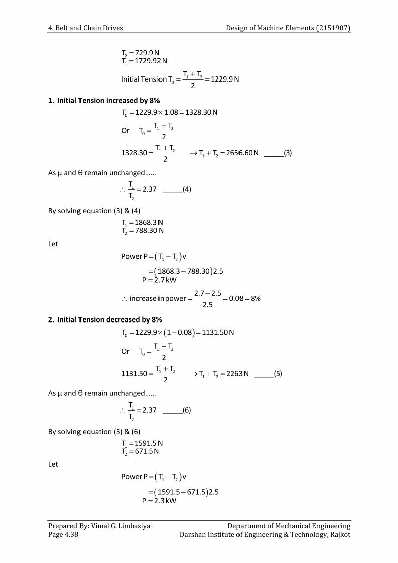
4. Belt and Chain Drives Design of Machine Elements (2151907)
Prepared By: Vimal G. Limbasiya Department of Mechanical Engineering Page 4.38 Darshan Institute of Engineering & Technology, Rajkot
2
1
T 729.9 NT 1729.92N
1 20
T TInitial Tension T 1229.9 N
2
1. Initial Tension increased by 8%
0T 1229.9 1.08 1328.30N
1 20
T TOr T
2
1 21 2
T T1328.30 T T 2656.60 N _____(3)
2
As µ and θ remain unchanged……
1
2
T2.37 _____(4)
T
By solving equation (3) & (4)
1
2
T 1868.3NT 788.30 N
Let
1 2Power P T T v
1868.3 788.30 2.5
P 2.7kW
2.7 2.5
increase inpower 0.08 8%2.5
2. Initial Tension decreased by 8%
0T 1229.9 1 0.08 1131.50N
1 20
T TOr T
2
1 21 2
T T1131.50 T T 2263N _____(5)
2
As µ and θ remain unchanged……
1
2
T2.37 _____(6)
T
By solving equation (5) & (6)
1
2
T 1591.5NT 671.5N
Let
1 2Power P T T v
1591.5 671.5 2.5
P 2.3kW

Design of Machine Elements (2151907) 4. Belt and Chain Drives
Department of Mechanical Engineering Prepared By: Vimal G. Limbasiya Darshan Institute of Engineering & Technology, Rajkot Page 4.39
2.5 2.3
decrease inpower 0.08 8%2.5
3. Angle of Lap (θ) is increased by 8% with same speed and T1
Let
110
2
T2.3log 0.3 165 1.08
T 180
1
2
T2.54
T
As T1 is same
1
2
T 1729.92NT 681.07N
1 2Power P T T v
1729.92 681.07 2.5
P 2.62kW
2.62 2.5
increase inpower 0.048 4.8%2.5
4. Coefficient of friction is increased by 8%
Let
110
2
T2.3log
T
0.3 1.08 165180
1
2
T2.54 _____(7)
T
Let
1 20
T TT 1229.9
2
1 2T T 2459.8N _____(8)
By solving equation (7) & (8)
2
1
T 694.9 NT 1764.9 N
Let
1 2Power P T T v
1764.9 694.9 2.5
P 2.67kW
2.67 2.5
increase inpower 0.07 7%2.5

4. Belt and Chain Drives Design of Machine Elements (2151907)
Prepared By: Vimal G. Limbasiya Department of Mechanical Engineering Page 4.40 Darshan Institute of Engineering & Technology, Rajkot
Example – 11:- In a belt drive the mass of belt is 1 kg/m length and its speed is 6 m/sec.
The drive transmits 9.6 kW of power. Determine the initial tension in the belt and strength
of belt. The coefficient of friction is 0.25 and angle of lap is 220°.
Solution:
3
0
m 1kg / m v 6 m / secP 9.6 10 WattT ?Strength ?
0.25
220 rad180
Let
1 2Power P T T v
1 29600 T T 6
1 2T T 1600N ______(1)
Let
110
2
T2.3log
T
0.25 220180
1
2
T2.31 _____(2)
T
Solving equation (1) & (2)
1
2
T 2594 NT 994 N
Let
2C
2Centrifugal Tension T m v
1(6) 36
N
1 20 C
T T 2594 994Initial Tension T T 36 1830 N
2 2
1 C
Strength of the belt Total Tension on tight sideT T2594 36 2630 N
Example – 12:-In an open bet drive, the diameters of larger and smaller pulley are 1.2 m
& 0.8 m respectively. The smaller pulley rotates at 320 rpm. The centre distance between
the shafts is 4 m. When stationary, the initial tension in the belt is 2.8 kN. The mass of the
belt is 1.8 kg/m and µ = 0.25. Determine the power transmitted.
Solution:
1 1
2 2
0
d 1.2m, N ?d 0.8 m, N 320 rpmx 4 m T 2800 Nm 1.8 kg / m 0.25Power ?

Design of Machine Elements (2151907) 4. Belt and Chain Drives
Department of Mechanical Engineering Prepared By: Vimal G. Limbasiya Darshan Institute of Engineering & Technology, Rajkot Page 4.41
2 2d N 0.8 320Velocity of Belt 13.40 m / sec
60 60
2C
2Centri T m v
1.8 (13fugal Tensi
.4) 3on
23.4 N
1 20 C
1 2
T TInitial Tension T T
2T T
2800 323.42
1 2T T 4953N _____(1)
For open belt drive
Angle of contact 180 2
180
1 2r r 0.6 0.4sin
X 42.86
180 2 2.86180
3.042rad
Let
110
2
T2.3log
T0.25 3.042
1
2
T2.14 _____(2)
T
By solving equation (1) & (2)
1
2
T 3376 NT 1577N
1 2Power P T T v
3376 1577 13.4 24106 Watt 24.10 kW
Example – 13:- The initial tension in a belt drive is found to be 600 N and the ratio of
friction tension is 1.8. The mass of the belt is 0.8 kg/m length. Determine the
1. Velocity of the belt for maximum power transmission
2. Tension on the tight side of the belt when it is started
3. Tension on the tight side of the belt when running at maximum speed.
Solution:
1. Velocity of the belt (v)
Let max power condition for initial tension
0T 600v 15.81m / sec
3m 3 0.8
2. Tension on tight side when belt is started v=0, TC = 0

4. Belt and Chain Drives Design of Machine Elements (2151907)
Prepared By: Vimal G. Limbasiya Department of Mechanical Engineering Page 4.42 Darshan Institute of Engineering & Technology, Rajkot
01
2 1.8 6002k TT 771.4 N
k 1 1.8 1
3. Tension on tight side when belt is running at max speed
0 C1
1
2 k T TT
k 12 1.8 600 199.7
1.8 1T 514.6 N
2C
2
T m v
0.8 15.8 199.7N
Or
1 2
0 C
T TT T
2with this equation you can solve the problem.
1 20 C
11
1
T TT T
2T
T1.8
600 199.72
T 514.6 N
Example – 14:- The driving pulley of an open belt drive is 800 mm diameter and rotates at
320 rpm while transmitting power to a driven pulley of 250 mm diameter. The Young’s
modulus of elasticity of the belt material is 110 N/mm2. Determine the speed lost by the
driven pulley due to creep if the stresses in the tight and slack sides of belt are found to be
0.8 N/mm2 and 0.32 N/mm2 respectively.
Solution:
1 1
22
21
22
OpenBelt DriveD 0.8 m, N 320 rpmD 0.250 mE 110 N / mm
0.8 N / mm0.32 N / mm
22 1
1 2 1
EN D( Velocity Ratio with creep )
N D E
2
110 0.32800N 320 1021rpm
250 110 0.8
Let velocity ratio without creep……
2 1
1 2
N D
N D
2
800N 320 1024 rpm
250
Speedlost due to creep 1024 1021 3rpm

Design of Machine Elements (2151907) 4. Belt and Chain Drives
Department of Mechanical Engineering Prepared By: Vimal G. Limbasiya Darshan Institute of Engineering & Technology, Rajkot Page 4.43
Example – 15:- The following data refers to flat belt drive
Power to be transmitted = 15 KW
Motor speed = 1440 r.p.m
Speed of driven pulley = 480 r.p.m.
Density of belt material = 950 Kg/m3
Centre distance between two pulleys = 810 mm
Belt speed = 20 m/sec
Modulus of elasticity for belt material = 100 MPa
Coefficient of friction = 0.35
Permissible stress for belt material = 2.25 MPa
Belt thickness = 5 mm
Calculate (i) pulley diameters (ii) length and width of the belt
Solution: P = 15 KW V = 20 m/sec
N1 = 1440 rpm Eb= 100 MPa
N2 = 480 rpm μ = 0.35
ρ = 950 Kg/ m3 σ = 100 MPa
c = 810 mm t = 5 mm
Velocity, 1 1
60
d NV
1(1440)
2060
d
d1 = 0.265 m
d1N1 = d2N2
0.265 x 1440 = d2(1440)
d2 = 0.795 m
Length of belt,
2
1 21 2
( )( ) 2
2 4
d dL d d c
c
2(0.795 0.265)(0.795 0.265) 2(0.81)
2 4 0.81L
L = 1.66 + 1.62 + 0.086
L = 3.36 m
2 1 0.3975 0.1325sin
0.81
r r
c
α = 19.09
= 180 – 2α
= 180 – 2(19.09)
= 141.82
= 141.82 x /180 = 2.47 rad

4. Belt and Chain Drives Design of Machine Elements (2151907)
Prepared By: Vimal G. Limbasiya Department of Mechanical Engineering Page 4.44 Darshan Institute of Engineering & Technology, Rajkot
1
2
Te
T
0.35 2.471
2
Te
T
1
2
2.37T
T
Power, P = (T1 – T2) V
15 x 103 = (T1 – T2) 20
T1 – T2 = 750
2.37 T2 – T2 = 750
T2 = 547.44 N
T1 = 1297.44 N
Mass of belt per meter length, m = Area x l x density
= b.t.l.ρ
= b x 0.005 x 1 x 950
= 4.75 b kg/m
Centrifugal tension, TC = mv2
= 4.75 b (20)2
= 1900 b
Maximum tension in belt, T = T1 + TC
σ.b.t = 1297.44 + 1900 b
2.25 x 10⁶ x b x 0.005 = 1297.44 + 1900 b
9350 b = 1297.44
b = 0.138 m
b ≈ 140 mm
Example – 16:- Determine the percentage increase in power capacity made possible in
changing over from a flat pulley to a V belt drive. The diameter of the flat pulleys is the same
as the pitch circle diameter of the V belt grooved pulleys. Pulley rotates at the same speed
as the grooved pulley. The belt materials are the same and they have the same cross
sectional area, with coefficient of friction for both as 0.3. The groove angle of the V belt
pulley is 600 and the angle of contact for both the cases is 1500.
Solution: d, N, material, area are same
μ = 0.3
2β = 60
= 150 x /180 = 2.6 rad
Flat belt
1
2
Te
T

Design of Machine Elements (2151907) 4. Belt and Chain Drives
Department of Mechanical Engineering Prepared By: Vimal G. Limbasiya Darshan Institute of Engineering & Technology, Rajkot Page 4.45
0.3 2.61
2
Te
T
1
2
2.18T
T
T1 = 2.18T2
Power transmitted by Flat belt, PF = (T1 – T2) V
= (2.18T2 – T2) V
= 1.18 T2 V
V-Belt
sin1
2
Te
T
0.3 2.6
1 sin30
2
Te
T
1
2
4.76T
T
T1 = 4.76T2
Power transmitted by V-belt, PV = (T1 – T2) V
= (4.76T2 – T2) V
= 3.76 T2 V
P PPercentage increase in power capacity = 100
PV F
F
3.76 1.18= 100
1.18
= 218.6 %
Example – 17:- Following data given for open V belt drive
Diameter of driving pulley =100 mm
Diameter of driven pulley = 200 mm
Center distance = 1000 mm
Groove angle = 40º
Mass of belt = 0.2 kg/m
Maximum permissible tension = 700 N
Coefficient of friction = 0.2
Plot a graph of maximum tension and power transmitted against belt velocity. Calculate
maximum power transmitted by belt and corresponding belt velocity. Neglect power losses.
Solution: d1 = 100 mm d2 = 200 mm

4. Belt and Chain Drives Design of Machine Elements (2151907)
Prepared By: Vimal G. Limbasiya Department of Mechanical Engineering Page 4.46 Darshan Institute of Engineering & Technology, Rajkot
c = 1 m
2β = 40 m = 0.2 kg/m T1 = 700 N
μ = 0.2
Arc of contact,
1 2 1180 2sin
2
d d
c
1 200 100
180 2sin2 1000
= 174.268
= 174.268 x /180 = 3.04 rad
2
sin12
2
T mVe
T mV
0.2 3.0421 sin20
22
T mVe
T mV
21
22
0.25.916
0.2
T V
T V …………..(a)
The belt tension is maximum when V = 0. For this condition,
1
2
5.916T
T
The maximum permissible tension is 700 N.
T1 = 700 N
T2 = 118.32 N
Initial tension,
1 2O
T T 700 118.32T
2 2
= 409.16 N
For maximum power transmission,
OT 409.16V
3m 3 0.2
= 26.11 m/s
T1 + T2 = 2TO
T1 + T2 = 818.32 …………….(b)
Substituting (V = 26.11 m/s) in Eq. (a),
21
22
0.2 (26.11)5.916
0.2 (26.11)
T
T …………….(c)
Solving Eq. (b) and (c)

Design of Machine Elements (2151907) 4. Belt and Chain Drives
Department of Mechanical Engineering Prepared By: Vimal G. Limbasiya Darshan Institute of Engineering & Technology, Rajkot Page 4.47
T2 = 215.24 N
T1 = 603.08 N
Power transmitted by belt, P = (T1 – T2) V
= (603.08 – 215.24) 26.11
= 10.126 kW
Variation of tension and power against belt velocity
For an intermediate velocity of V = 10 m/s,
21
22
0.2 (10)5.916
0.2 (10)
T
T …………….(d)
Solving Eq. (b) and (d),
T2 = 132.54 N
T1 = 685.78 N
Power transmitted by belt, P = (T1 – T2) V
= (685.78 – 132.54) 10
= 5.532 kW
For an intermediate velocity of V = 40 m/s,
21
22
0.2 (40)5.916
0.2 (40)
T
T …………….(d)
Solving Eq. (b) and (d),
T2 = 345.78 N
T1 = 472.53 N
Power transmitted by belt, P = (T1 – T2) V
= (472.53 – 345.78) 40
= 5.07 kW
Similar calculations can be made for other values of the belt velocity and plot a graph of
maximum tension and power transmitted against belt velocity.

4. Belt and Chain Drives Design of Machine Elements (2151907)
Prepared By: Vimal G. Limbasiya Department of Mechanical Engineering Page 4.48 Darshan Institute of Engineering & Technology, Rajkot
Fig. 4.22
Example – 18:- 11 KW, 1440 rpm motor is used to transmit power through V belt drive
having following details.
Each belt has area of cross section = 140 mm2
Groove angle for pulley = 380
Density of belt material = 1350 Kg/m3
Diameter of pulley on motor shaft = 140 mm
Speed ratio = 2:1
Centre distance = 400 mm
Maximum permissible stress for belt = 2.5 MPa
Coefficient of friction between belt and pulley = 0.25
Find the number of belts required.
Solution: P = 11 KW d1= 140mm
N1 = 1440 rpm V.R. = 2:1
A = 140 mm2 c = 400 mm
2β = 38 σ = 2.5MPa
ρ = 1350 Kg/ m3 μ = 0.25
Velocity, 1 1
60
d NV
0.140 1440
60V
V = 10.55 m/sec

Design of Machine Elements (2151907) 4. Belt and Chain Drives
Department of Mechanical Engineering Prepared By: Vimal G. Limbasiya Darshan Institute of Engineering & Technology, Rajkot Page 4.49
1 2
2 1
N d
N d
0.140 x 2 = d2
d2 = 0.28 m
2 1 0.28 0.14
sin0.4
r r
c
α = 20.487
= 180 – 2α
= 180 – 2(20.487)
= 139.025
= 139.025 x/180 = 2.426 rad
Mass of belt per meter length, m = Area x l x density
= 140 x 10–6 x 1 x 1350
= 0.189 kg/m
Maximum tension in belt, T = T1 + TC
σ.A = T1 + mv2
2.5 x 140 = T1 + 0.189(10.55)2
T1 = 328.96 N
sin1
2
Te
T
0.25 2.426
1 sin19
2
Te
T
1
2
6.44T
T
T2 = 51.06 N
Power transmitted by belt, P = (T1 – T2) V
= (328.96 – 51.06) 10.55
= 2.93 KW
Total power transmittedNo. of belts =
Power transmitted per belt
11No. of belts =
2.93
= 3.75
≈ 4 belts
Example–19:- Select a HI-SPEED belt for a light machine tool form following given data:
Power = 14.5 KW Motor speed = 1440 r.p.m.
Machine pulley speed = 360 r.p.m. Load factor = 1.2

4. Belt and Chain Drives Design of Machine Elements (2151907)
Prepared By: Vimal G. Limbasiya Department of Mechanical Engineering Page 4.50 Darshan Institute of Engineering & Technology, Rajkot
Centre distance between pulley = 1000 mm Open belt drive
Load rating for belt = 0.023 KW per mm per width per ply at 1800 arc of contact at10
m/sec belt speed
Preferable pulley sizes: 200,224,250,280,315,400,450,500,560,630,710,800,900,1000
mm
Arc of contact (degree) 120 130 140 150 160
Arc of contact factor 1.33 1.26 1.19 1.13 1.08
No. of ply Standard width of belt in mm
4-ply 40 44 50 63 76 90 100 112 125 152
5-ply 76 100 112 125 152
6-ply 112 125 152 180 200
Solution: P = 14.5 KW
N1 = 1440 rpm
N2 = 360 rpm
Fa = 1.2
c = 1 m
load rating for belt = 0.023 KW
V = 10 m/sec
Diameter of smaller and bigger pulleys
Velocity, 1 1
60
d NV
1(1440)
1060
d
d1 = 0.133 m = 133 mm
Selecting the preferred pulley diameter of 200 mm.
d1N1 = d2N2
200 x 1440 = d2(360)
d2 = 800mm
Maximum power, Pmax = Fa.P
= 1.2 x 14.5
= 17.4 KW
Arc of contact,
1 2 1180 2sin
2
d d
c
1 800 200
180 2sin2 1000

Design of Machine Elements (2151907) 4. Belt and Chain Drives
Department of Mechanical Engineering Prepared By: Vimal G. Limbasiya Darshan Institute of Engineering & Technology, Rajkot Page 4.51
= 145.084
Related Arc of contact factor, Fd = 1.16
Corrected Power, Pco = Fd x Pmax
= 1.16 x 17.4
= 20.184 KW
Corrected power
Width No. of plies = Load rating for belt
20.184 =
0.023
= 877.56
Belt widths,
4 plies 877.56
219.39 mm4
b
5 plies 877.56
175.5 mm5
b
6 plies 877.56
146.26 mm6
b
We should select belt of 152 mm preferred width and 6 plies.
Example – 20:- Design a V- belt drive from the following data:
Power to be transmitted = 7.5 kW
Motor speed = 1440 r.p.m.
Speed of driven pulley = 480 r.p.m
Centre distance between two pulleys = 1000 mm
Service factor = 1.3
Driver pulley diameter = 200 mm.
Arc of contact (degree) 151 154 157 160 163
Arc of contact factor 0.93 0.93 0.94 0.95 0.96
Correction factor for belt length
Belt Length (mm)
A B C
1.09 2480 3200 5380
1.10 2570 – –
1.11 2700 3600 –
Solution: P = 7.5 kW
N1 = 1440 rpm
N2 = 480 rpm
c = 1 m
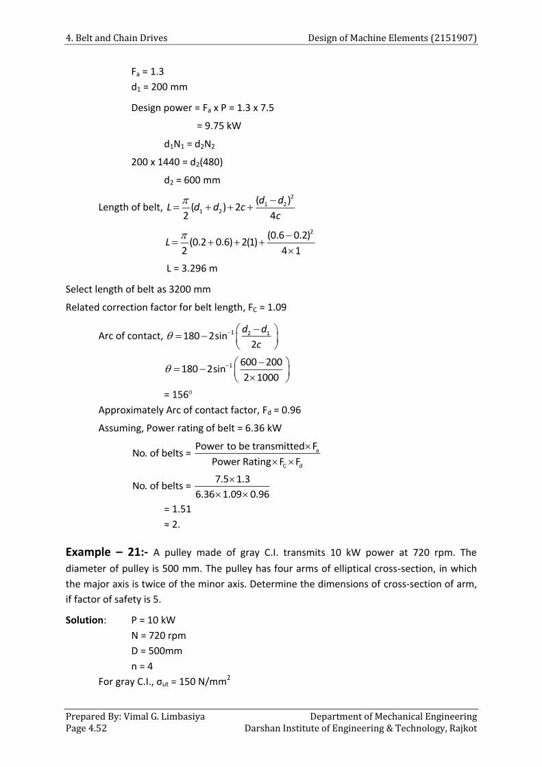
4. Belt and Chain Drives Design of Machine Elements (2151907)
Prepared By: Vimal G. Limbasiya Department of Mechanical Engineering Page 4.52 Darshan Institute of Engineering & Technology, Rajkot
Fa = 1.3
d1 = 200 mm
Design power = Fa x P = 1.3 x 7.5
= 9.75 kW
d1N1 = d2N2
200 x 1440 = d2(480)
d2 = 600 mm
Length of belt,
2
1 21 2
( )( ) 2
2 4
d dL d d c
c
2(0.6 0.2)(0.2 0.6) 2(1)
2 4 1L
L = 3.296 m
Select length of belt as 3200 mm
Related correction factor for belt length, FC = 1.09
Arc of contact,
1 2 1180 2sin
2
d d
c
1 600 200
180 2sin2 1000
= 156
Approximately Arc of contact factor, Fd = 0.96
Assuming, Power rating of belt = 6.36 kW
a
C d
Power to be transmitted FNo. of belts =
Power Rating F F
7.5 1.3No. of belts =
6.36 1.09 0.96
= 1.51
≈ 2.
Example – 21:- A pulley made of gray C.I. transmits 10 kW power at 720 rpm. The
diameter of pulley is 500 mm. The pulley has four arms of elliptical cross-section, in which
the major axis is twice of the minor axis. Determine the dimensions of cross-section of arm,
if factor of safety is 5.
Solution: P = 10 kW
N = 720 rpm
D = 500mm
n = 4
For gray C.I., σut = 150 N/mm2

Design of Machine Elements (2151907) 4. Belt and Chain Drives
Department of Mechanical Engineering Prepared By: Vimal G. Limbasiya Darshan Institute of Engineering & Technology, Rajkot Page 4.53
Power,
t2 NMP
60
3 t2 720 M
10 1060
Mt = 132.63 x 10³ N.mm
One half of arms carry the load at any instance, tangential force at end of each arm,
Tangential force,
3tM 132.63 10
P 265.26 Nn 4
R 2502 2
Bending moment, Mb = P x R
= 265.26 x 250
= 66315 N.mm
For an elliptical cross-section with a & b as minor and major axis
3I ab64
, b = 2a
3 4I a(2a) a64 8
y = b/2 = a
bb
My
I
4
6631530 a
a8
a = 17.78 mm ≈ 20 mm
b = 40 mm
Example – 22:- An overhung cast iron pulley transmits 7.5 kW at 400 r.p.m. The belt
drive is vertical and angle of wrap may be taken as 1800. Find:
(i) Diameter of the pulley. The density of CI is 7200 kg/m3
(ii) Width of the belt, if the co-efficient of friction between the belt and the pulley
is 0.25 assuming thickness t = 10 mm.
(iii) Diameter of the shaft, if the distance of the pulley center line from the nearest
bearing is 300 mm.
(iv) Dimensions of the key for securing the pulley on to the shaft.
(v) Size of the arms six in number.
The section of the arms may be taken as elliptical, the major axis being twice the minor
axis. The following stresses may be taken for design purpose: Shaft and key: 80
MPa(Tension), 50 MPa (Shear); Belt: 2.5 MPa (Tension); Pulley rim: 4.5 MPa (Tension);
Pulley arms: 15 MPa (Tension).
Solution: P = 7.5 kW N = 400 rpm
= 180 ρCI = 7200 kg/m3

4. Belt and Chain Drives Design of Machine Elements (2151907)
Prepared By: Vimal G. Limbasiya Department of Mechanical Engineering Page 4.54 Darshan Institute of Engineering & Technology, Rajkot
μ = 0.25 t = 10 mm
L = 300 mm n = 6
Shaft and Key – σt = 80 MPa,
τ = 50 MPa
Belt – σt = 2.5 MPa
Pulley rim – σt = 4.5 MPa
Pulley arms – σt = 15 MPa
Diameter of pulley
Centrifugal stress or tensile stress induced in pulley rim
σt = ρV2
4.5 x 106 = 7200 V2
V = 25 m/s
Velocity,
60
dNV
(400)
2560
d
d = 1.19 m
Width of belt
1
2
Te
T
0.25 3.141
2
Te
T
1
2
2.19T
T
Power, P = (T1 – T2) V
7.5 x 103 = (T1 – T2) 25
T1 – T2 = 300
2.19 T2 – T2 = 300
T2 = 252.1 N
T1 = 552.1 N
Assuming the leather belt for which density of belt may be taken as 1000 kg/m3
Mass of belt per meter length, m = b x t x l x density
= b.t.l.ρ
= b x 0.01 x 1 x 1000
= 10 b kg/m

Design of Machine Elements (2151907) 4. Belt and Chain Drives
Department of Mechanical Engineering Prepared By: Vimal G. Limbasiya Darshan Institute of Engineering & Technology, Rajkot Page 4.55
Centrifugal tension, TC = mv2
= 10 b (25)2
= 6250 b
Maximum tension in belt, T = T1 + TC
σ.b.t = 552.1 + 6250 b
2.5 x 10⁶ x b x 0.01 = 552.1 + 6250 b
18750 b = 552.1
b = 0.029 m
b ≈ 30 mm
Diameter of the shaft
Power,
t2 NMP
60
3 t2 400 M
7.5 1060
Torque, Mt = 179 N.m
Bending moment on shaft due to tensions of belt,
M = (T1 + T2 + 2TC) L
= [552.1 + 252.1 + 2 x 10 x 0.3 x (25)2] 0.3
= 353.76 N.m
Equivalent twisting moment, 2 2eT T M
2 2eT (179) (353.76)
Te = 396.47 N.m
3eT d
16
3 3396.47 10 d 5016
d = 34.31 mm
d ≈ 38 mm
Dimension of the key
The standard dimensions of the key for 38 mm shaft diameter
Width of key, w = 12 mm
Thickness of key, t = 8 mm
Mt = l x w x τ x d/2
179 x 103 = l x 12 x 50 x 38/2
l = 15.7 mm

4. Belt and Chain Drives Design of Machine Elements (2151907)
Prepared By: Vimal G. Limbasiya Department of Mechanical Engineering Page 4.56 Darshan Institute of Engineering & Technology, Rajkot
Length of the key should be equal to hub length
Length of key, l = d./2 = 38./2
= 59.7 mm
Size of arms
Minor axis of elliptical cross-section of arms
3t 33
b
M 179 10a 1.72 1.72
n 6 15
= 21.63 mm
≈ 22 mm
Major axis, b = 2a =2 x 22
= 44 mm
Example – 23:- A pulley of 0.9m diameter transmits 7.5 kW power at 200 rpm. Find the
width of a leather belt if maximum tension is not to exceed 14.5 N per mm width. The
tension in the tight side is twice that in the slack side. Also determine the dimensions of the
various parts of the flat belt pulley, assuming it to have six arms. The arms are of C.I. for
which tensile stress may be taken as 15 N/mm2. The diameter of the shaft is 35 mm.
Solution: D = 0.9 m P = 7.5 kW
N = 200 rpm T = 14.5 N per mm width
T1 = 2T2 n = 6
σt = 15 MPa d = 35 mm
Velocity,
60
DNV
0.9 200
60V
V = 9.42 m/s
Power, P = (T1 – T2) V
7.5 x 103 = (T1 – T2) 9.42
T1 – T2 = 796.18
2T2 – T2 = 796.18
T2 = 796.18 N
T1 = 1592.3 N
Maximum tension is 14.5 N per mm width
b = T1/14.5 = 1592.3 / 14.5
= 109.8 mm
≈ 110 mm

Design of Machine Elements (2151907) 4. Belt and Chain Drives
Department of Mechanical Engineering Prepared By: Vimal G. Limbasiya Darshan Institute of Engineering & Technology, Rajkot Page 4.57
Width of Pulley, B = 1.25 b
= 137.5 mm
Thickness of pulley rim for single belt
D 900
t 3 3200 200
= 7.5 mm ≈ 8 mm
Power,
t2 NMP
60
3 t2 200 M
7.5 1060
Torque, Mt = 358.098 N.m
Assuming the cross-section of arms as elliptical with major axis equal to twice minor axis
b1 = 2a1
3t 33
1
b
M 358.098 10a 1.72 1.72
n 6 15
a1= 27.25 mm ≈ 30 mm
b1 = 60 mm
Diameter of hub, d1 = 1.5 d + 25 = (1.5 x 35) + 25
= 77.5 mm
Length of hub, L = d./2 = 35./2
= 54.97 mm ≈ 55 mm
Since the length of hub should not less than 2/3B
2 2
L B 137.53 3
= 92 mm
4.18 Design of chain drives
A chain drive consists of an endless chain wrapped around two sprockets.
A chain can be defined as a series of links connected by a pin joints.
The sprocket is a toothed wheel with a special profile for the teeth.
The chain drive is intermediate between belt and gear drives. It has some features of
belt drives and some of gear drives.
Pitch of chain: It is distance between the hinge centre of a link and the
corresponding hinge centre of adjacent link.
Pitch circle diameter of sprocket chain: It is the diameter of an imaginary circle that
passes through the centre of link pins as the chain is wrapped on sprocket.

4. Belt and Chain Drives Design of Machine Elements (2151907)
Prepared By: Vimal G. Limbasiya Department of Mechanical Engineering Page 4.58 Darshan Institute of Engineering & Technology, Rajkot
Advantages
1. Constant velocity due to no slip, so it is positive drive.
2. No effect on overload on the velocity ratio.
3. Oil or grease on the surface does not affect the velocity ratio.
4. Chains occupy less space as they made of metals.
5. Lesser loads are put on the shaft.
6. High transmission efficiency due to “No slip”.
7. Through one chain only motion can be transmitted to several shaft.
Disadvantages
1. It is heavier as compared to the belt.
2. There is gradual stretching and increase in length of chains. From time to time some of its
links have to be removed.
3. Lubrication of its parts is required.
4. Chains are costlier compared to belts.
Classification of Chains
1. Hoisting Chain
Hoisting chain includes oval link and stud link chains. An oval link is a common form of
hoisting chain. It consists of a oval link and is also known as coil chain. Such chains are used
for lower speed only.
Fig. 4.23 Hoisting Chain
2. Conveyor Chain
Conveyor chain may be detachable or hook type or closed joint type. The sprocket teeth are
so shaped that the chain should run onto and off the sprocket smoothly without
interference.
Such chains are used for low speed agricultural machinery. The material of the link is usually
malleable cast iron. The motion of the chain is not very smooth.

Design of Machine Elements (2151907) 4. Belt and Chain Drives
Department of Mechanical Engineering Prepared By: Vimal G. Limbasiya Darshan Institute of Engineering & Technology, Rajkot Page 4.59
Fig. 4.24 Conveyor Chain
3. Power transmission Chain
These chains are made of steel in which the wearing parts are hardened. They are
accurately machined and run on carefully designed sprockets.
1. Block Chain: - This type of chain is mainly used for
transmission of power at low speeds. Sometimes they
are also used as conveyor chains in place of malleable
conveyor chains. Fig. 4.25 Block Chain
2. Roller Chain: - A common form of a roller chain
is shown in figure. A bushing is fixed to a inner
link whereas the outer link has a pin fixed to it.
There is only sliding motion between pin and
bushing.
The roller is made of a hardened material and is
free to turn on the bushing.
Fig. 4.26 Roller Chain
3. Silent Chain (Inverted tooth chain):- Though roller
chain can run quietly at fairly high speed. The silent
chains are used where maximum quietness is
desired. Silent chains do not have rollers. The links
are so shaped as to engage directly with the
sprocket teeth. The included angle is either 60° or
75°.
Fig. 4.27 Silent Chain
Geometric Relationships (Relation between Pitch and Pitch circle diameter
for Chain)
The engagement of chain on sprocket wheel is shown in Fig. 4.8. D is the pitch circle
diameter of the sprocket and α is called the pitch angle. The pitch circle diameter of the

4. Belt and Chain Drives Design of Machine Elements (2151907)
Prepared By: Vimal G. Limbasiya Department of Mechanical Engineering Page 4.60 Darshan Institute of Engineering & Technology, Rajkot
sprocket is defined as the diameter of an imaginary circle that passes through the centres of
link pins as the chain is wrapped on the sprocket.
Fig. 4.28
360
z ……………..(a)
where z is the number of teeth on the sprocket. From the figure, it can be proved that
(p / 2)sin
2 (D / 2)
pD
sin2
pD
180sin
z
.....................(b)
The velocity ratio i ofthe chain drives is given by
1 2
2 1
n zi
n z
Wheren1, n2 = speeds of rotation of driving and driven shafts (rpm)
z1,z2= number of teeth on driving and driven sprockets.
The average velocity of the chain is given by,
60 60
Dn zpnV
…………….(c)
Where, V is the average velocity in m/s.
The length of the chain is always expressed in terms of the number of links, or
L = Ln x p ……………(d)
Where, L = length of the chain (mm)
Ln = number of links in the chain
The number of links in the chain is by the following approximate relationships:

Design of Machine Elements (2151907) 4. Belt and Chain Drives
Department of Mechanical Engineering Prepared By: Vimal G. Limbasiya Darshan Institute of Engineering & Technology, Rajkot Page 4.61
2
1 2 1 2n
z z z za pL 2
p 2 2 a
…………..(e)
where, a = centre distance between axes of driving and driven sprockets (mm)
z1 = number of teeth on the smaller sprocket
z2 = number of teeth on the larger sprocket
The above formula is derived by analogy with the length of the belt. The first two
terms represent the number of links when (z1 = z2) and the sides of the chain are parallel.
The third term takes into consideration the inclination of the sides. It is obvious that the
chain should contain a whole number of links. Therefore, the number of links (Ln) is adjusted
to the previous or next digit so as to get an even number. It is always preferred to have an
'even' number of links, since the chain consists of alternate pairs of inner and outer link
plates.
When the chain has an odd number of links, an additional link, called 'offset' link, is
provided. The offset link is, however, weaker than the main links. After selecting the exact
number of links, the centre to centre distance between the axes of the two sprockets is
calculated by the following formula:
2 2
1 2 1 2 1 2n n
z z z z z zpa L L 8
4 2 2 2
…………(f)
The above equation can be easily derived from Eq. (e). The centre distance calculated by the
formula does not provide any sag. In practice, a small amount of sag is essential for the links
to take the best position on the sprocket wheel. The centre distance is, therefore, reduced
by a margin of (0.002a to 0.004a) to account for the sag.
Polygonal Effect
The chain passes around the sprocket as a series of chordal links. This action is similar to
that of a non-slipping belt wrapped around a rotating polygon. The chordal action is
illustrated in Figure 4.8, where the sprocket has only four teeth. It is assumed that the
sprocket is rotating at a constant speed of n rpm. In Fig. 4.9, the chain link AB is at a distance
of (D/2) from the centre of the sprocket wheel and its linear velocity is given by,
max /60
Dn
V m s
As the sprocket rotates through an angle (α/2), the position of the chain link AB is shown in
Figure 4.8. In this case, the link is at a distance of (D/2) x cos(α/2) from the centre of the
sprocket and its linear velocity is given by,
min
cos2
/60
Dn
V m s

4. Belt and Chain Drives Design of Machine Elements (2151907)
Prepared By: Vimal G. Limbasiya Department of Mechanical Engineering Page 4.62 Darshan Institute of Engineering & Technology, Rajkot
Fig. 4.29 Polygonal action of chain
It is evident that the linear speed of the chain is not uniform but varies from Vmax to Vmin
during every cycle of tooth engagement. This results in a pulsating and jerky motion. The
variation in velocity is given by
max min(V V ) ∝ 1 cos2
max min(V V ) ∝ 180
1 cosz
As the number of teeth (z) increases to ∞, cos (180/z) or cos (180/∞), i.e., cos (0°) will
approach unity and (Vmax - Vmin) will become zero. Therefore, the variation will be zero. In
order to reduce the variation in chain speed, the number of teeth on the sprocket should be
increased.
It has been observed that the speed variation is 4% for a sprocket with 11 teeth, 1.6% for a
sprocket with 17 teeth, and less than 1% for a sprocket with 24 teeth.
For smooth operation at moderate and high speeds, it is considered a good practice to use a
driving sprocket with at least 17 teeth.
From durability and noise considerations, the minimum number of teeth on the driving
sprocket should be 19 or 21.
Power Rating of Roller Chains
The power transmitted by the roller chain can be expressed by the elementary equation
P = T1.V
Where, T1 = allowable tension in the chain (N)
V = average velocity of chain (m/s),
The Power rating of the chain is determined by the following relationship:

Design of Machine Elements (2151907) 4. Belt and Chain Drives
Department of Mechanical Engineering Prepared By: Vimal G. Limbasiya Darshan Institute of Engineering & Technology, Rajkot Page 4.63
S
1 2
Power to be transmitted KPower rating of chain =
K K
Where, KS = service factor
K1 = multiple strand factor
K2 = tooth correction factor
The service factor takes into consideration the effect of shocks and vibrations on the
power to be transmitted.
The tooth correction factor K2 accounts for the variation in teeth.
There are duplex and triplex chains too. The variation in the number strands is taken
into accounts by the multiple strand factor K1.
Modes of chain failure
There are four modes of chain failures
(i) Wear: The wear of the chain is caused by the articulation of pins in the bushings.
The wear results in elongation of the chain, or in other words, the chain pitch is
increased. This makes the chain 'ride out' on the sprocket teeth, resulting in a
faulty engagement. When the elongation is excessive, it becomes necessary to
replace the chain. The permissible elongation for the chain is 1.5 to 2.5%. When the
chain is properly lubricated, a layer of oil film between the contacting surfaces of
the pin and the bushing reduces wear.
(ii) Fatigue: As the chain passes around the sprocket wheel, it is subjected to a tensile
force, which varies from a maximum on the tight side to a minimum on the loose
side. The chain link is, therefore, subjected to one complete cycle of fluctuating
stresses during every revolution of the sprocket wheel. This results in a fatigue
failure of side link plates. For infinite life, the tensile stress should be lower than
the endurance limit of the link plates.
(iii) Impact: The engagement of rollers with the teeth of the sprocket results in impact.
When excessive, this may lead to the breakage of roller or bushing. Increasing the
number of teeth on the sprocket or reducing chain tension and speed reduces the
magnitude of the impact force.
(iv) Galling: Galling is a stick-slip phenomenon between the pin and the bushing. When
the chain tension is high, welds are formed at the high spots of the contacting area.
Such microscopic welds are immediately broken due to relative motion of
contacting surfaces and leads to excessive wear, even in the presence of the
lubricant.

4. Belt and Chain Drives Design of Machine Elements (2151907)
Prepared By: Vimal G. Limbasiya Department of Mechanical Engineering Page 4.64 Darshan Institute of Engineering & Technology, Rajkot
Example – 24:- The center to Centre distance between two sprockets of a chain drive is
600 mm. The chain drive is used to reduce the speed from 180 rpm to 90 rpm on the driving
sprocket has 18 teeth and a pitch circle diameter of 480 mm. Determine
1. No. of teeth on the driven sprocket
2. Pitch and the length of chain.
Solution:
1 1
2 2
C Centre distance between sprocket 600 mmN 180 rpm ,z 18 teethN 90 rpm ,z ?
1.
2 1 12 1
1 2 2
N Z Nz z
N Z N180
18 36 Teeth90
2. Pitch of chain (p)
2
180 180p 2R sin 2 0.240 sin 0.04183m 41.83mm
z 36
3. Length of chain (L)
No. of links in chain, 2
1 2 2 1n
z z z z2a pL
p 2 2 a
2
n
2 600 18 36 36 18 41.83L
41.83 2 2 600
Ln = 56.26
= 56 links
Length of chain, L = Ln x p
L = 56 x 41.83
= 2342.48 mm
Example – 25:- A simple chain No. 10B is used to transmit power from a 1400 rpm electric
motor to a line shaft running at 350 rpm. The number of teeth on the driving sprocket wheel
is 19. The operation is smooth without any shocks. Calculate: (i) The rated power for which
the chain drive is recommended. (ii) The tension in the chain for this rated power; and (iii)
The factor of safety for the chain based on the breaking load.
Use following data:
At 1400 rpm, for chain 10B, power rating is 11.67 kW,
Service factor KS: 1.3, Multiple strand factor K1: 1.0, Breaking Load: 22200 N,

Design of Machine Elements (2151907) 4. Belt and Chain Drives
Department of Mechanical Engineering Prepared By: Vimal G. Limbasiya Darshan Institute of Engineering & Technology, Rajkot Page 4.65
Tooth correction factor K2: 1.11, Pitch: 15.875 mm.
Solution: N = 1400 rpm z = 19
1 2
S
Power rating K KPower to be transmitted =
K
11.67 1 1.11P =
1.3
P = 9.96 kW
Velocity,60
zpN
V
319 15.875 10 1400
60
V
V = 7.038 m/s
The tension in the chain, 3
1
P 9.96 10T
V 7.038
= 1415.17 N
Breaking Load
F.O.S.Chain Tension
22200
F.O.S.1415.17
= 15.68.
Example – 26:- A chain drive with double strands of 16B type has a pitch of 25.4 mm. It is
used to transmit power between a 15 tooth driving sprocket rotating at 700 rpm and a 60
tooth driven sprocket. For the drive conditions, a service factor of 1.3 can be used. Find
(i) The power that can be transmitted by the drive.
(ii) Length of the chain, if the centre distance between the sprockets is 475 mm.
Use the following data:
At 700 rpm, for chain 16B, power rating is 27.73 kW.
No. of strands The multiple strand factor , K1
1 1.0
2 1.7
3 2.5
4 3.3
No. of teeth Tooth correction factor , K2
15 0.85
60 2.80
Solution: p = 25.4 mm z1 = 15

4. Belt and Chain Drives Design of Machine Elements (2151907)
Prepared By: Vimal G. Limbasiya Department of Mechanical Engineering Page 4.66 Darshan Institute of Engineering & Technology, Rajkot
N = 700 rpm z2 = 60
KS = 1.3 a = 475 mm
Power rating = 27.73 kW.
1 2
S
Power rating K KPower to be transmitted =
K
27.73 1.7 0.85P =
1.3
P = 30.82 kW
No. of links in chain, 2
1 2 2 1n
z z z z2a pL
p 2 2 a
2
n
2 475 15 60 60 15 25.4L
25.4 2 2 475
Ln = 77.64
= 78 links
Length of chain, L = Ln x p
L = 78 x 25.4
= 1981.2 mm
Example – 27:- It is required to design a chain drive to connect a 12 kW, 1400 rpm electric
motor to a centrifugal pump running at 700 rpm. The service condition involves moderate
shock. Pitch is 19.05 mm
(i) Determine the P.C.D. of driving and driven sprocket.
(ii) Determine no. of chain links.
(iii) Specify the correct center distance between the axes of sprockets.
Solution: P = 12 kW
N1 = 1400 rpm
N2 = 700 rpm
p = 19.05 mm
P.C.D. for driving sprocket, 1
1
p 19.05D
180180 sinsin17Z
= 103.67 mm
Z1N1 = Z2N2
12 1
2
NZ Z
N

Design of Machine Elements (2151907) 4. Belt and Chain Drives
Department of Mechanical Engineering Prepared By: Vimal G. Limbasiya Darshan Institute of Engineering & Technology, Rajkot Page 4.67
2
1400Z 17
700
= 34
For driven sprocket, 2
2
p 19.05D
180180 sinsin34Z
= 206.463 mm
The centre distance between sprocket wheel should be between (30p) to (50p). Taking a
mean value (40p).
The approximate centre distance, a = 40 p = 40 x 19.05
= 762 mm
No. of links in chain, 2
1 2 2 1n
Z Z Z Z2a pL
p 2 2 a
2
n
2 762 17 34 34 17 19.05L
19.05 2 2 762
Ln = 106 links
Correct centre distance,
2 2
1 2 1 2 2 1n n
z z z z z zpa L L 8
4 2 2 2
2 219.05 17 34 17 34 34 17
a 106 106 84 2 2 2
= 765.026 mm
To provide small slag, for allowing chain links to take the best position on the sprocket
teeth, the centre distance is reduced by (0.002a).
Correct centre distance is given by
a = 0.998 x 765.026
= 763.49 mm
Example – 28:- Select a simple roller chain drive to transmit 5 kW power 1400 r.p.m. from
an electric motor to a drilling machine.
Speed reduction = 3:1
Approximate centre distance = 500 mm
Service factor = 1.3
Assume moderate shock conditions.
Number of teeth on pinion = 21

4. Belt and Chain Drives Design of Machine Elements (2151907)
Prepared By: Vimal G. Limbasiya Department of Mechanical Engineering Page 4.68 Darshan Institute of Engineering & Technology, Rajkot
Also find no. of chain links and correct centre distance.
Power rating (kW) of a simple roller chain
Pinion Speed (r.p.m.) 08A 08B 10A
1000 3.94 5.09 8.05
1400 5.28 6.81 11.18
Solution: P = 5 kW N1 = 1400 rpm
a = 500 mm i = 3
KS = 1.3 z = 21
For single strand chain, K1 = 1
For 21 teeth, K2 = 1.26
1 2
S
Power rating K KPower to be transmitted =
K
Power rating 1 1.265 =
1.3
Power rating = 5.16 kW
Referring to Table, the power rating of the chain 8A at 1400 rpm is 5.28 kW. Therefore the
chain number 8A is selected.
Assume pitch, p = 12.70 mm
z2 = i z1 = 3 x 21 =63
No. of links in chain, 2
1 2 2 1n
z z z z2a pL
p 2 2 a
2
n
2 500 21 63 63 21 12.70L
12.70 2 2 500
Ln = 121.87 ≈ 122 links
Correct centre distance,
2 2
1 2 1 2 2 1n n
z z z z z zpa L L 8
4 2 2 2
2 212.70 21 63 21 63 63 21
a 122 122 84 2 2 2
= 500.81 mm

Department of Mechanical Engineering Prepared By: Mr. SUNIL G. JANIYANI Darshan Institute of Engineering & Technology, Rajkot Page 5.1
5 PRESSURE VESSELS
Course Contents
5.1 Introduction to Pressure
Vessels
5.2 General Materials for
Pressure Vessels
5.3 Classification of Pressure
Vessels
5.4 Stresses in a Thin Cylindrical
Shell Due to an Internal
Pressure
5.5 Thin Spherical Shells
Subjected to an Internal
Pressure
5.6 Thick Cylindrical Shells
Subjected to an Internal
Pressure
5.7 Autofrettage or Pre-stressing
5.8 Types of End Closures
5.9 Gaskets and Gasketed Joint
Examples

5. PRESSURE VESSELS Design of Machine Elements (2151907)
Prepared By: Mr. SUNIL G. JANIYANI Department of Mechanical Engineering Page 5.2 Darshan Institute of Engineering & Technology, Rajkot
5.1 Introduction to Pressure Vessels
Vessels, tanks, and pipelines that carry, store, or receive fluids are called pressure
vessels.
A pressure vessel is defined as a container with a pressure differential between
inside and outside. The inside pressure is usually higher than the outside, except for
some isolated situations.
Fig 5.1 Typical Components of Pressure Vessels
The fluid inside the vessel may undergo a change in state as in the case of steam
boilers, or may combine with other reagents as in the case of a chemical reactor.
Pressure vessels often have a combination of high pressures together with high
temperatures, and in some cases flammable fluids or highly radioactive materials.
Because of such hazards it is imperative that the design be such that no leakage can
occur.
In addition these vessels have to be designed carefully to cope with the operating
temperature and pressure.
It should be borne in mind that the rupture of a pressure vessel has a potential to
cause extensive physical injury and property damage. Plant safety and integrity are
of fundamental concern in pressure vessel design.
5.1.1 Applications of Pressure Vessels
Industrial compressed air receivers
Domestic hot water storage tanks
Diving cylinders (Scuba diving)
Recompression chambers
Distillation towers
Autoclaves (In medical industry to sterilize)
Oil refineries and petrochemical plants
Nuclear reactor vessels

Design of Machine Elements (2151907) 5. PRESSURE VESSLES
Department of Mechanical Engineering Prepared By: Mr. SUNIL G. JANIYANI Darshan Institute of Engineering & Technology, Rajkot Page 5.3
Pneumatic and Hydraulic Reservoirs
Storage vessels for liquefied gases such as ammonia, chlorine, propane,
butane and LPG.
5.1.2 ASME Codes for Pressure Vessels
It is a standard that provides rules for the design, fabrication, and inspection
of boilers and pressure.
This establishes and maintains design, construction and inspection standards
providing for maximum protection of life and property.
ASME Section VIII : Boiler and Pressure Vessel Code (BPVC)
Division 1 - Rules for Construction of Pressure Vessels
Division 2 - Alternative Rules
Division 3 - Alternative Rules for Construction of High Pressure Vessels
5.2 General Materials for Pressure Vessels
The materials that are used in pressure vessel construction are:
Steels
Nonferrous materials such as aluminum and copper
Metals such as titanium and zirconium
Nonmetallic materials, such as, plastic, composites and concrete
Metallic and nonmetallic protective coatings
Various materials has some typical characteristics as below:
Carbon steel: strength & moderate corrosion resistance
Low-alloy steels: strength at high temperatures
Stainless steels: corrosion resistance
Nickel alloys: corrosion resistance
Copper alloys: sea water resistance
Aluminum: light, low temperature toughness
Titanium: sea water, chemical resistance
Refractories: very high temperatures
Non-metallic: corrosion & chemicals
5.2.1 Factors Affecting Selection of Material:
Factors Affecting Selection of Material are as following:
Process fluids (i.e. a plastic might be perfect for the fluid corrosiveness,
but will melt when the operators ‘steam’ the equipment during cleaning)
Operating temperature
Operating pressure
Fluid Velocity
Contamination of product
Required life of the equipment (May choose to incur shorter life and
replace more often)
Cost of the materials of construction (base material + fabrication costs)

5. PRESSURE VESSELS Design of Machine Elements (2151907)
Prepared By: Mr. SUNIL G. JANIYANI Department of Mechanical Engineering Page 5.4 Darshan Institute of Engineering & Technology, Rajkot
5.3 Classification of Pressure Vessels
Based on Wall Thickness:
1) Thin Wall Vessel
2) Thick Wall Vessel
Based on Geometric Shapes:
1) Cylindrical Vessels
2) Spherical Vessels
3) Rectangular Vessels
4) Combined Vessels
Based on Installation Methods:
1) Vertical Vessels
2) Horizontal Vessels
Based on Operating Temperature:
1) Low Temperature Vessels (less than or equal to - 20° C)
2) Normal Temperature Vessels (Between - 20° C to 150° C)
3) Medium Temperature Vessels (Between 150° C to 450° C)
4) High Temperature Vessels (more than or equal to 450° C)
Based on Design Pressure:
1) Low Pressure Vessels (0.1 MPa to 1.6 MPa)
2) Medium Pressure Vessels (1.6 MPa to 10 MPa)
3) High Pressure Vessels (10 MPa to 100 MPa)
4) Ultra High Pressure Vessels (More than 100 MPa)
Based on Technological Processes:
1) Reaction Vessel
2) Heat Exchanger Vessel
3) Separation Vessel
4) Storage Container Vessel
5.3.1 Difference Between Thin Shell and Thick shell Pressure Vessels
The pressure vessels, according to their dimensions, may be classified as thin
shell or thick shell.
If the wall thickness of the shell (t) is less than 1/10 to 1/15 of the diameter of
the shell (d), then it is called a thin shell. On the other hand, if the wall
thickness of the shell is greater than 1/10 to 1/15 of the diameter of the shell,
then it is said to be a thick shell.
Thin shells are used in boilers, tanks and pipes, whereas thick shells are used
in high pressure cylinders, tanks, gun barrels etc.
Another criterion to classify the pressure vessels as thin shell or thick shell is
the internal fluid pressure (p) and the allowable stress (σ t).
If the internal fluid pressure (p) is less than 1/6 of the allowable stress, then it
is called a thin shell. On the other hand, if the internal fluid pressure is
greater than 1/6 of the allowable stress, then it is said to be a thick shell.

Design of Machine Elements (2151907) 5. PRESSURE VESSLES
Department of Mechanical Engineering Prepared By: Mr. SUNIL G. JANIYANI Darshan Institute of Engineering & Technology, Rajkot Page 5.5
5.4 Stresses in a Thin Cylindrical Shell due to an Internal Pressure
The analysis of stresses induced in a thin cylindrical shell are made on the following
assumptions:
1) The effect of curvature of the cylinder wall is neglected.
2) The tensile stresses are uniformly distributed over the section of the walls.
3) The effect of the restraining action of the heads at the end of the pressure
vessel is neglected.
When a thin cylindrical shell is subjected to an internal pressure, it is likely to fail in
the following two ways:
1) It may fail along the longitudinal section (i.e. circumferentially) splitting the
cylinder into two troughs, as shown in Fig 5.2.
2) It may fail across the transverse section (i.e. longitudinally) splitting the
cylinder into two cylindrical shells, as shown in Fig 5.3.
Thus the wall of a cylindrical shell subjected to an internal pressure has to withstand
tensile stresses of the following two types: (a) Circumferential or hoop stress, and (b)
Longitudinal stress.
5.4.1 Circumferential or Hoop Stress
Fig 5.2 (a) View of Shell (b) Cross-section of Shell
Consider a thin cylindrical shell subjected to an internal pressure as shown in the
figure above.
Tensile stress acting in a direction tangential to the circumference is called
circumferential or hoop stress.
In other words, it is a tensile stress on longitudinal section (or on the cylindrical
walls).
Let p = Intensity of internal pressure,
d = Internal diameter of the cylindrical shell,
l = Length of the cylindrical shell,
t = Thickness of the cylindrical shell, and
σt1 = Circumferential or hoop stress for the material of the cylindrical shell.
We know that the total force acting on a longitudinal section (i.e. along the diameter
X-X) of the shell
= Intensity of pressure × Projected area
Also the total resisting force acting on the cylinder walls for two sections
=

5. PRESSURE VESSELS Design of Machine Elements (2151907)
Prepared By: Mr. SUNIL G. JANIYANI Department of Mechanical Engineering Page 5.6 Darshan Institute of Engineering & Technology, Rajkot
Equating equations (i) and (ii), we have
5.4.2 Longitudinal Stress
Fig 5.3 (a) View of Shell (b) Cross-section of Shell
Consider a closed thin cylindrical shell subjected to an internal pressure as shown in
the above figure.
Tensile stress acting in the direction of the axis is called longitudinal stress .
In other words, it is tensile stress acting on the transverse or circumferential section
Y-Y (or on the ends of the vessel).
Let σt2 = Longitudinal stress.
In this case, the total force acting on the transverse section (i.e. along Y-Y)
= Intensity of pressure × Cross-sectional area
Also the total resisting force
=
Equating equations (i) and (ii), we have
5.5 Thin Spherical Shells Subjected to an Internal Pressure
Fig 5.4 Thin Spherical Shell
Consider a thin spherical shell subjected to an internal pressure as shown in the
above figure.

Design of Machine Elements (2151907) 5. PRESSURE VESSLES
Department of Mechanical Engineering Prepared By: Mr. SUNIL G. JANIYANI Darshan Institute of Engineering & Technology, Rajkot Page 5.7
Let V = Storage capacity of the shell,
p = Intensity of internal pressure,
d = Diameter of the shell,
t = Thickness of the shell,
σt = Permissible tensile stress for the shell material.
In designing thin spherical shells, we have to determine the diameter of the shell and
the thickness of the shell.
We know that the storage capacity of the shell,
(
)
(
)
As a result of the internal pressure, the shell is likely to rupture along the centre of
the sphere.
Therefore force tending to rupture the shell along the centre of the sphere or
bursting force
= Pressure × Area
Also resisting force of the shell
= Stress × Resisting area
=
Equating equations (i) and (ii), we have
5.6 Thick Cylindrical Shells Subjected to an Internal Pressure
When the ratio of the inner diameter (d) of the cylinder to the wall thickness (t) is
less than 10 to 15, the cylinder is called as thick cylinder.
Hydraulic cylinders, high pressure pipes and gun barrels are examples of thick
cylinders.
The radial stress (σr) is neglected in thin cylinders, while it is of significant magnitude
in case of thick cylinders.
There are number of equations for the design of thick cylinders. The choice of
equation depends upon two parameters: Cylinder material (whether brittle or
ductile) and Condition of cylinder ends (open or closed).
In the design of thick cylindrical shells, the following equations are mostly used:

5. PRESSURE VESSELS Design of Machine Elements (2151907)
Prepared By: Mr. SUNIL G. JANIYANI Department of Mechanical Engineering Page 5.8 Darshan Institute of Engineering & Technology, Rajkot
1. Lame’s equation,
2. Birnie’s equation,
3. Clavarino’s equation and
4. Barlow’s equation.
5.6.1 Lame's Equation
When the material of the cylinder is brittle, such as cast iron or cast steel,
Lame’s equation is used to determine the wall thickness.
It is based on the maximum principal stress theory of failure, where
maximum principal stress is equated to permissible stress for the material.
Three principal stresses at the inner surface of the cylinder are as follows:
(
)
(
)
(
)
Therefore,
Hence σt is the criterion of design. From equation (ii)
(
)
(
)
(
) (
)
(
)
√
Substituting in the above equation
√
√
√

Design of Machine Elements (2151907) 5. PRESSURE VESSLES
Department of Mechanical Engineering Prepared By: Mr. SUNIL G. JANIYANI Darshan Institute of Engineering & Technology, Rajkot Page 5.9
√
where
5.6.2 Birnie’s equation
In case of open-end cylinders (such as pump cylinders, rams, gun barrels etc.)
made of ductile material (i.e. low carbon steel, brass, bronze, and aluminium
alloys), the allowable stresses cannot be determined by means of maximum-
stress theory of failure.
In such cases, the maximum-strain theory is used. According to this theory,
the failure occurs when the strain reaches a limiting value.
Birnie’s equation for the wall thickness of a cylinder,
[√
]
5.6.3 Clavarino’s equation
This equation is also based on the maximum-strain theory of failure, but it is
applied to closed-end cylinders (or cylinders fitted with heads) made of
ductile material.
According to this equation, the thickness of a cylinder,
[√
]
where
5.6.4 Barlow’s equation
This equation is generally used for high pressure oil and gas pipes.
According to this equation, the thickness of a cylinder,
where, Do is outer diameter of cylinder
5.7 Autofrettage or Pre-stressing
Autofrettage is a process of pre-stressing the cylinder before using it in service.
It is used in case of high-pressure cylinders and gun barrels.
When the cylinder is subjected to internal pressure, the circumferential stress (σ t) at
the inner surface limits the pressure capacity of the cylinder.
In the pre-stressing process, residual compressive stresses are developed at the
inner surface.

5. PRESSURE VESSELS Design of Machine Elements (2151907)
Prepared By: Mr. SUNIL G. JANIYANI Department of Mechanical Engineering Page 5.10 Darshan Institute of Engineering & Technology, Rajkot
When the cylinder is loaded in service, the residual compressive stresses at the inner
surface begin to decrease, become zero and finally become tensile as the pressure is
gradually increased.
Autofrettage increases the pressure capacity of the cylinder.
It has another advantage that the residual compressive stresses close the cracks
within the cylinder resulting in increased endurance strength.
There are three methods of pre-stressing the cylinder. They are as follows:
1. Compound cylinder: It consists of two concentric cylinders with outer cylinder
shrunk onto the inner one. This induces compressive stresses in the inner
cylinder. Compound cylinder is extensively used in practice.
(a) Compounded Cylinder (b) Cylinder (c) Jacket
Fig 5.5 Compound Cylinder
A compound cylinder, consisting of a cylinder and a jacket is shown in figure
(a). The inner diameter of the jacket is slightly smaller than the outer
diameter of the cylinder.
When the jacket is heated, it expands sufficiently to move over the cylinder.
As the jacket cools, it tends to contract onto the inner cylinder, which induces
residual compressive stresses.
There is a shrinkage pressure P between the cylinder and the jacket.
The pressure P tends to contract the cylinder and expand the jacket, as
shown in figures (b) and (c).
The shrinkage pressure P can be evaluated from the below equation for a
given amount of interference (δ).
[
(
)
(
) (
)]
The resultant stresses in a compound cylinder are found by superimposing
the two stresses-stresses due to shrink fit and those due to internal pressure.
2. Overloading the cylinder: The second method consists of overloading the
cylinder before it is put into service.
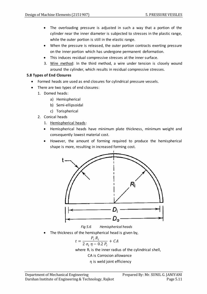
Design of Machine Elements (2151907) 5. PRESSURE VESSLES
Department of Mechanical Engineering Prepared By: Mr. SUNIL G. JANIYANI Darshan Institute of Engineering & Technology, Rajkot Page 5.11
The overloading pressure is adjusted in such a way that a portion of the
cylinder near the inner diameter is subjected to stresses in the plastic range,
while the outer portion is still in the elastic range.
When the pressure is released, the outer portion contracts exerting pressure
on the inner portion which has undergone permanent deformation.
This induces residual compressive stresses at the inner surface.
3. Wire method: In the third method, a wire under tension is closely wound
around the cylinder, which results in residual compressive stresses.
5.8 Types of End Closures
Formed heads are used as end closures for cylindrical pressure vessels.
There are two types of end closures:
1. Domed heads:
a) Hemispherical
b) Semi-ellipsoidal
c) Torispherical
2. Conical heads
1. Hemispherical heads:
Hemispherical heads have minimum plate thickness, minimum weight and
consequently lowest material cost.
However, the amount of forming required to produce the hemispherical
shape is more, resulting in increased forming cost.
Fig 5.6 Hemispherical heads
The thickness of the hemispherical head is given by,
where Ri is the inner radius of the cylindrical shell,
CA is Corrosion allowance
η is weld joint efficiency

5. PRESSURE VESSELS Design of Machine Elements (2151907)
Prepared By: Mr. SUNIL G. JANIYANI Department of Mechanical Engineering Page 5.12 Darshan Institute of Engineering & Technology, Rajkot
2. Semi-ellipsoidal Heads:
In a semi-ellipsoidal head, the ratio of the major axis to the minor axis is
taken as 2:1.
Fig 5.7 Semi-ellipsoidal Heads
The thickness of a semi-ellipsoidal head is given by,
From the above equations, it is observed that the thickness of the semi-
elliptical head is more (almost twice) than the corresponding hemispherical
head, and to that extent, the material cost is more.
However due to the shallow dished shape, the forming cost is reduced.
The length of the straight portion (Sf) is given by,
Sf =3 t or 20 mm (whichever is more)
3. Torispherical Heads:
Torispherical heads are extensively used as end closures for a large variety of
cylindrical pressure vessels.
Fig 5.8 Torispherical Heads
They are shaped by using two radius – the crown radius L and knuckle radius
ri.

Design of Machine Elements (2151907) 5. PRESSURE VESSLES
Department of Mechanical Engineering Prepared By: Mr. SUNIL G. JANIYANI Darshan Institute of Engineering & Technology, Rajkot Page 5.13
The crown radius L is the radius of the dish that constitutes the major portion
of the head.
The knuckle radius ri is the corner radius joining the spherical crown with the
cylindrical shell.
Torispherical heads require less forming than semi-ellipsoidal heads.
Their main drawback is the local stresses at the two discontinuities namely
the junction between “the crown head and the knuckle radius” and the
junction between “the knuckle radius and the cylindrical shell”.
The localised stresses may lead to failure due to brittle fracture.
The thickness of a torispherical head is given by,
The knuckle radius ri is taken as 6% of the crown radius, ri = 0.06 L
4. Conical Heads:
Fig 5.9 Conical Heads
The thickness of a conical head is given by,
where, α is half the apex angle.
The half apex angle is usually less than 30⁰.
5.9 Gaskets and Gasketed Joints
A gasket is a device used to create and maintain a barrier against the transfer of fluid
across the mating surfaces of a mechanical assembly. It is used in static joints, such
as cylinder block and cylinder head.
There are two types of gaskets-metallic and non-metallic.
Metallic gaskets consist of sheets of lead, copper or aluminium.
Non-metallic gaskets are made of asbestos, cork, rubber or plastics.

5. PRESSURE VESSELS Design of Machine Elements (2151907)
Prepared By: Mr. SUNIL G. JANIYANI Department of Mechanical Engineering Page 5.14 Darshan Institute of Engineering & Technology, Rajkot
Metallic gaskets are used for high temperature and high pressure applications. They
can have corrugated construction or they can be made in the form of plain sheets.
The limiting temperatures of metallic gaskets are as follows:
Lead: 90° C
Copper/brass: 250° C
Aluminium: 400° C
The metallic gasket takes a permanent set when compressed in assembly and there
is no recovery to compensate for separation of contact faces.
They are also susceptible to corrosion and chemical atmosphere. Their performance
also depends upon surface finish of the contacting surfaces.
Asbestos gaskets have excellent resistance to be crushing loads and cutting action
due to sharp edges of the flanges. Dimensional stability is another advantage.
They are used in cylinder head, water and steam pipe fittings and manifold
connections.
Vulcanized compounds of rubber and cork are employed as gaskets in steam lines,
combustion chambers and chemical environment.
They are used for applications involving irregular surfaces. They are of low cost, but
are affected by fungus and alkalis.
Rubber compounds have excellent impermeability and ability to flow into joint
imperfections when compressed.
Asbestos gaskets can be used up to 250° C, while other non-metallic gaskets have a
limiting temperature of 70° C.
Fig 5.10 Shapes of Gasket
Different shapes of gasket for cylinder head are illustrated in the above figure.


