Embed Size (px)
Citation preview

INTRODUCTION TO LIE ALGEBRAS AND THEIRREPRESENTATIONS
PART IIIMICHAELMAS 2010
IAN GROJNOWSKIDPMMS, UNIVERSITY OF CAMBRIDGE
[email protected] BY ELENA YUDOVINA
STATISTICAL LABORATORY, UNIVERSITY OF [email protected]
1. Introduction, motivation, etc.
Lecture 1 For most of this lecture, we will be motivating why we care about Lie algebrasand why they are defined the way they are. If there are sections of it that don’t make sense,they can be skipped (although if none of it makes sense, you should be worried).
Connected Lie groups are groups which are also differentiable manifolds. The simplealgebraic groups over algebraically closed fields (which is a nice class of Lie groups) are:
SL(n) = A ∈ Mat n| det A = 1SO(n) = A ∈ SLn|AAT = ISP (n) = A ∈ SLn|some symplectic form...
and exactly 5 others (as we will actually see!)
(We are ignoring finite centers, so Spin(n), the double cover of SO(n), is missing.)
Remark. Each of these groups has a maximal compact subgroup. For example, SU(n) is themaximal compact subgroup of SL(n), while SOn(R) is the maximal compact subgroup ofSOn(C). These are themselves Lie groups, of course. The representations of the maximalcompact subgroup are the same as the algebraic representations of the simple algebraic groupare the same as the finite-dimensional representations of its (the simple algebraic group’s)Lie algebra – which are what we study.
Lie groups complicated objects: for example, SU2(C) is homotopic to a 3-sphere, and SUn
is homotopic to a twisted product of a 3-sphere, a 5-sphere, a 7-sphere, etc. Thus, studyingLie groups requires some amount of algebraic topology and a lot of algebraic geometry. Wewant to replace these “complicated” disciplines by the “easy” discipline of linear algebra.
Therefore, instead of a Lie group G we will be considering g = TIG, the tangent space toG at the identity.
Definition. A linear algebraic group is a subgroup of some GLn defined by polynomialequations in the matrix coefficients.
We see that the examples above are linear algebraic groups.
Date: Michaelmas 2010.1

2 IAN GROJNOWSKI
Remark. It is not altogether obvious that this is an intrinsic characterisation (it wouldbe nice not to depend on the embedding into GLn). The intrinsic characterisation is as“affine algebraic groups,” that is, groups which are affine algebraic varieties and for whichmultiplication and inverse are morphisms of affine algebraic varieties. One direction of thisidentification is relatively easy (we just need to check that multiplication and inverse reallyare morphisms); in the other direction, we need to show that any affine algebraic group hasa faithful finite-dimensional representation, i.e. embeds in GL(V ). This involves looking atthe ring of functions and doing something with it.
We will now explain a tangent space if you haven’t met with it before.
Example 1.1. Let’s pretend we’re physicists, since we’re in their building anyway. LetG = SL2, and let |ε| 1. Then for
g =
(1
1
)+ ε
(a bc d
)+ higher-order terms
to lie in SL2, we must have det g = 1, or
1 = det
(1 + εa εb
εc 1 + εd
)+ h.o.t = 1 + ε(a + d) + ε2(junk) + h.o.t
Therefore, to have g ∈ G we need to have a + d = 0.
To do this formally, we define the dual numbers
E = C[ε]/ε2 = a + bε|a, b ∈ CFor a linear algebraic group G, we consider
G(E) = A ∈ Mat n(E)|A satisfies the polynomial equations defining G ⊂ GLnFor example,
SL2(E) = (
α βγ δ
)|α, β, γ, δ ∈ E, αδ − βγ = 1
The natural map E → C, ε 7→ 0 gives a projection π : G(E)→ G. We define the Lie algebraof G as
g ∼= π−1(I) ∼= X ∈ Mat n(C)|I + εX ∈ G(E).In particular,
sl2 = (
a bc d
)∈ Mat 2(C)|a + d = 0.
Remark. I + Xε represents an “infinitesimal change at I in the direction X”. Equivalently,the germ of a curve Spec C[[ε]]→ G.
Exercise 1. (Do this only if you already know what a tangent space and tangent bundleare.) Show that G(E) = TG is the tangent bundle to G, and g = T1G is the tangent spaceto G at 1.
Example 1.2. Let G = GLn = A ∈ Mat n|A−1exists.Claim:
G(E) := A ∈ Mat n(E)|A−1exists= A + Bε|A, B ∈ Mat nC, A−1exists
Indeed, (A + Bε)(A−1 − A−1BA−1ε) = I.
INTRODUCTION TO LIE ALGEBRAS AND THEIR REPRESENTATIONS PART III MICHAELMAS 20103
Remark. It is not obvious that GLn is itself a linear algebraic group (what are the polynomialequations for “determinant is non-zero”?). However, we can think of GLn ⊂ Mat n+1 as
(
Aλ
)| det(A)× λ = 1.
Example 1.3. G = SLnC.
Exercise 2. det(I + εX) = 1 + ε · trace (X)
As a corollary to the exercise, sln = X ∈ Mat n|trace (X) = 0.
Example 1.4. G = OnC = AAT = I. Then
g := X ∈ Mat nC|(I + εX)(I + εX)T = I= X ∈ Mat nC|I + ε(X + XT ) = I= X ∈ Mat nC|X + XT = 0
the antisymmetric matrices. Now, if X + XT = 0 then 2 × trace (X) = 0, and since we’reworking over C and not in characteristic 2, we conclude trace (X) = 0. Therefore, this isalso the Lie algebra of SOn.
This is not terribly surprising, because topologically On has two connected componentscorresponding to determinant +1 and −1 (they are images of each other via a reflection).Since g = T1G, it cannot see the det = −1 component, so this is expected.
The above example propmts the question: what exactly is it in the structure of g that weget from G being a group?
The first thing to note is that g does not get a multiplication. Indeed, (I +Aε)(I +Bε) =I + (A + B)ε, which has nothing to do with multiplication.
The bilinear operation that turns out to generalize nicely is the commutator, (P, Q) 7→PQP−1Q−1. Taken as a map G × G → G that sends (I, I) 7→ I, this should give a mapT1G× T1G→ T1G by differentiation.
Remark. Generally, differentiation gives a linear map, whereas what we will get is a bilinearmap. This is because we will in fact differentiate each coordinate: i.e. first differentiate themap fP : G→ G, Q 7→ PQP−1Q−1 with respect to Q to get a map fP : g→ g (with P ∈ Gstill) and then differentiate again to get a map g× g→ g.
What is this map?Let P = I + Aε, Q = I + Bδ where ε2 = δ2 = 0 but εδ 6= 0. Then
PQP−1Q−1 := (I + Aε)(I + Bδ)(I − Aε)(I −Bδ)
= I + (AB −BA)εδ.
Thus, the binary operation on g should be [A, B] = AB −BA.
Definition. The bracket of A and B is [A, B] = AB −BA.
Exercise 3. Show that (PQP−1Q−1)−1 = QPQ−1P−1 implies [A, B] = −[B, A], i.e. thebracket is skew-symmetric.
Exercise 4. Show that the associativity of multiplication in G implies the Jacobi identity
0 = [[X, Y ], Z] + [[Y, Z], X] + [[Z,X], Y ]
4 IAN GROJNOWSKI
Remark. The meaning of “implies” in the above exercises is as follows: we want to think of thebracket as the derivative of the commutator, not as the explicit formula [A, B] = AB −BA(which makes the skew-symmetry obvious, and the Jacobi identity only slightly less so). Forexample, we could have started working in a different category.
We will now define our object of study.
Definition. Let K be a field, char K 6= 2, 3. A Lie algebra g is a vector space over Kequipped with a bilinear map (Lie bracket) [, ] : g× g→ g with the following properties:
(1) [X, Y ] = −[Y,X] (skew-symmetry);(2) [[X, Y ], Z] + [[Y, Z], X] + [[Z,X], Y ] = 0 (Jacobi identity).
Lecture 2 Examples of the Lie algebra definition from last time:
Example 1.5. (1) gln = Mat n with [A, B] = AB −BA.(2) son = A + AT = 0(3) sln = trace (A) = 0 (note that while trace (AB) 6= 0 for A, B ∈ sln, we do have
trace (AB) = trace (BA), so [A, B] ∈ sln even though AB 6∈ sln)
(4) sp2n = A ∈ gl2n|JAT J−1+A = 0 where J is the symplectic form
1. . .
1−1
. . .−1
(5) b =
∗ ∗ . . . ∗∗ . . . ∗
. . ....∗
∈ gln the upper triangular matrices (the name is b for Borel,
but we don’t need to worry about that yet)
(6) n =
0 ∗ . . . ∗
0 . . . ∗. . .
...0
∈ gln the strictly upper triangular matrices (the name is n
for nilpotent, but we don’t need to worry about that yet)(7) For any vector space V , let [, ] : V × V → V be the zero map. This is the “abelian
Lie algebra”.
Exercise 5. (1) Check directly that gln is a Lie algebra.(2) Check that the other examples above are Lie subalgebras of gln, that is, vector
subspaces closed under [, ].
Example 1.6.
(∗ ∗∗ 0
)is not a Lie subalgebra of gl2.
Exercise 6. Find the algebraic groups whose Lie algebras are given above.
Exercise 7. Classify all Lie algebras of dimension 3. (You might want to start with di-mension 2. I’ll do dimension 1 for you on the board: skew symmetry of bracket means thatbracket is zero, so there is only the abelian one.)
INTRODUCTION TO LIE ALGEBRAS AND THEIR REPRESENTATIONS PART III MICHAELMAS 20105
Definition. A representation of a Lie algebra g on a vector space V is a homomorphism ofLie algebras φ : g→ glV . We say that g acts on V .
Observe that, above, our Lie algebras were defined with a (faithful) representation in tow.There is always a representation coming from the Lie algebra acting on itself (it is the
derivative of the group acting on itself by conjugation):
Definition. For x ∈ g define ad (x) : g→ g as y 7→ [x, y].
Lemma 1.1. ad : g→ End g is a representation (called the adjoint representation).
Proof. We need to check whether ad ([x, y]) = ad (x)ad (y) − ad (y)ad (x), i.e. whether theequality will hold when we apply it to a third element z. But:
ad ([x, y])(z) = [[x, y], z]
and
ad (x)ad (y)(z)− ad (y)ad (x)(z) = [x, [y, z]]− [y, [x, z]] = −[[y, z], x]− [[z, x], y].
These are equal by the Jacobi identity.
Definition. The center of g is x ∈ g : [x, y] = 0, ∀y ∈ g = ker(ad : g→ End g).
Thus, if g has no center, then ad is an embedding of g into End g (and conversely, ofcourse).
Is it true that every finite-dimensional Lie algebra embeds into some glV , i.e. is lin-ear? (Equivalently, is it true that every finite-dimensional Lie algebra has a faithful finite-dimensional representation?) We see that if g has no center, then the adjoint representation
makes this true. On the other hand, if we look inside gl2, then n =
(0 ∗0 0
)is abelian, so
maps to zero in gln, despite the fact that we started with n ⊂ gl2. That is, we can’t alwaysjust take ad .
Theorem 1.2 (Ado’s theorem; we will not prove it). Any finite-dimensional Lie algebraover K is a subalgebra of gln, i.e. admits a faithful finite-dimensional representation.
Remark. This is the Lie algebra equivalent of the statement we made last time about algebraicgroups embedding into GL(V ). That theorem was “easy” because there was a naturalrepresentation to look at (functions on the algebraic group). There isn’t such a naturalobject for Lie groups, so Ado’s theorem is actually hard.
Example 1.7. g = sl2 with basis e =
(0 10 0
), h =
(1 00 −1
), f =
(0 01 0
)(these are the
standard names). Then [e, f ] = h, [h, e] = 2e, and [h, f ] = −2f .
Exercise 8. Check this!
A representation of sl2 is a triple E, F, H ∈ Mat n satisfying the same bracket relations.Where might we find such a thing?
In this lecture and the next, we will get them as derivatives of representations of SL2. Wewill then rederive them from just the linear algebra.
Definition. If G is an algebraic group, an algebraic representation of G on V is a homomor-phism of groups ρ : G→ GL(V ) defined by polynomial equations in the matrix coefficients.
6 IAN GROJNOWSKI
(This can be done so that it is invariant of the embedding into GLn. Think about it.)To get a representation of the Lie algebra out of this, we again use the dual numbers E. If
we use E = K[ε]/ε2 instead of K, we will get a homomorphism of groups G(E)→ GLV (E).Moreover, since ρ(I) = I and it commutes with the projection map, we get
ρ(I + Aε) = I + ε× (some function of A) = I + εdρ(A)
(this is to be taken as the definition of dρ(A)).
Exercise 9. dρ is the derivative of ρ evaluated at I (i.e., dρ : TIG→ TIGLV ).
Exercise 10. The fact that ρ : G→ GLV was a group homomorphism means that dρ : g→glV is a Lie algebra homomorphism, i.e. V is a representation of g.
Example 1.8. G = SL2.Let L(n) be the space of homogeneous polynomials of degree n in two variables x, y, with
basis xn, xn−1y, . . . , xyn−1, yn (so dim L(n) = n + 1). Then GL2 acts on L(n) by change of
coordinates: for g =
(a bc d
)and f ∈ L(n) we have
((ρng)f)(x, y) = f(ax + cy, bx + dy)
In particular, ρ0 is the trivial representation of GL2, ρ1 is the usual 2-dimensional represen-tation K2, and
ρ2
(a bc d
)=
a2 ab b2
2ac ad + bc 2bdc2 cd d2
Since GL2 acts on L(n), we see that SL2 acts on L(n).
Remark. The proper way to think of this is as follows. GL2 acts on P1 and on O(n) on P1,hence on the global sections Γ(O(n), P1) = SnK2. That’s the source of these representations.We can do this sort of thing for all the other algebraic groups we listed previously, using flagvarieties instead of P1 and possibly higher (co)homologies instead of the global sections (thisis a theorem of Borel, Weil, and Bott). That, however, requires algebraic geometry, and getsharder to do in infinitely many dimensions.
Differentiating the above representations, e.g. for e =
(0 10 0
), we see
ρ(I + εe)xiyj = xi(εx + y)j = xiyj + εjxi+1yj−1
Therefore, dρ(e)xiyj = jxi+1yj−1,
Exercise 11. (1) In the action of the Lie algebra,
e(xiyj) = jxi+1yj−1
f(xiyj) = ixi−1yj+1
h(xiyj) = (i− j)xiyj.
(2) Check directly that these formulae give a representation of sl2.(3) Check that L(2) is the adjoint representation.(4) Show that the formulae e = x ∂
∂y, f = y ∂
∂x, h = x ∂
∂x− y ∂
∂ygive an (infinite-
dimensional!) representation of sl2 on k[x, y].
INTRODUCTION TO LIE ALGEBRAS AND THEIR REPRESENTATIONS PART III MICHAELMAS 20107
(5) Let char (k) = 0. Show that L(n) is an irreducible representation of sl2, hence ofSL2.
Lecture 3 Last time we defined a functor
(algebraic representations of a linear algebraic group G)→(Lie algebra representations of g = Lie (G))
via ρ 7→ dρ.This functor is not as nice as you would like to believe, except for the Lie algebras we care
about.
Example 1.9. G = C× =⇒ g = Lie (G) = C with [x, y] = 0.A representation of g = C on V is a matrix A ∈ End (V ) (to ρ : C→ End (V ) corresponds
A = ρ(1)).W ⊆ V is a submodule iff AW ⊆ W , and ρ is isomorphic to ρ′ : g → End (V ′) iff A and
A′ are conjugate as matrices.Therefore, representations of g correspond to the Jordan normal form of matrices.As any linear transformation over C has an eigenvector, there’s always a 1D subrep of V .
Therefore, V is irreducible iff dim V = 1. Also, V is completely decomposable (a direct sumof irreducible representations) iff A is diagonalizable.
For example, if A =
0 1
0 1. . . . . .
. . . 10
then the associated representation is indecom-
posable, but not irreducible. Invariant subspaces are 〈e1〉, 〈e1, e2〉, . . . , 〈e1, e2, . . . , en〉, andnone of them has an invariant orthogonal complement.
Now let’s look at the representations of G = C×.The irreducible representations are ρn : G→ GL1 = Aut(C) via z 7→ (multiplication by) zn
for n ∈ Z. Every finite-dimensional representation is a direct sum of these.
Remark. Proving these statements about representations of G takes some theory of algebraicgroups. However, you probably know this for S1, which is homotopic to G. Recall that toget complete reducibility in the finite group setting you took an average over the group; youcan do the same thing here, because S1 is compact and so has finite volume. In fact, for thetheory that we study, our linear algebraic groups have maximal compact subgroups, whichhave the same representations, which for this reason are completely reducible. We will notprove that representations of the linear algebraic groups are the same as the representationsof their maximal compact subgroups.
Observe that the representations of G and of g are not the same. Indeed, ρ 7→ dρ willsend ρn 7→ n ∈ C (prove it!). Therefore, irreducible representations of G embed into ir-reducible representations of g, but the map is not remotely surjective (not to mention thedecomposability issue).
The above example isn’t very surprising, since g is also the Lie algebra Lie (C, +), and weshould not expect representations of g to coincide with those of C×. The surprising result is
8 IAN GROJNOWSKI
Theorem 1.3 (Lie). ρ 7→ dρ is an equivalence of categories RepG→ Rep g if G is a simplyconnected simple algebraic group.
Remark. A “simple algebraic group” is not simple in the usual sense: e.g. SLn has a center,which is obviously a normal subgroup. However, if G is simply connected and simple in theabove sense, then the center of G is finite (e.g. ZSLn = µn, the nth roots of unity), and thenormal subgroups are subgroups of the center.
Exercise 12. If G is an algebraic group, and Z is a finite central subgroup of G, thenLie (G/Z) = Lie (G). (Morally, Z identifies points “far away”, and therefore does not affectthe tangent space at I.)
We have now seen that the map (algebraic groups) → (Lie algebras) is not injective (seeabove exercise, or – more shockingly – G = C, C×). In fact,
Exercise 13. Let Gn = C× n C where C× acts on C via t · λ = tnλ (so (t, λ)(t′, λ′) =(tt′, t′nλ + λ′)). Show that Gn
∼= Gm iff n = ±m. Show that Lie (Gn) ∼= Cx + Cy with[x, y] = y independently of n.
The map also isn’t surjective (its image are the “algebraic Lie algebras”). This is easilyseen in characteristic p; for example, slp/center cannot be the image of an algebraic group.In general, algebraic groups have a Jordan decomposition – every element can be written as(semisimple)× (nilpotent), – and therefore the algebraic Lie algebras should have a Jordandecomposition as well. In Bourbaki, you can find an example of a 5-dimensional Lie algebra,for which the semisimple and the nilpotent elements lie only in the ambient glV and not inthe algebra as well.
2. Representations of sl2
From now on, all algebras and representations are over C (an algebraically closed field ofcharacteristic 0). Periodically we’ll mention which results don’t need this.
Recall the basis of sl2 was e =
(0 10 0
), h =
(1 00 −1
), and f =
(0 01 0
)with commutation
relations [e, f ] = h, [h, e] = 2e, [h, f ] = −2f .For the next while, we will be proving the following
Theorem 2.1.
(1) For all n ≥ 0 there exists a unique irreducible representation of g = sl2 of dimensionn + 1. (Recall L(n) from the previuos lecture; these are the only ones.)
(2) Every finite-dimensional representation of sl2 is a direct sum of irreducible represen-tations.
Let V be a representation of sl2.
Definition. The λ-weight space for V is Vλ = v ∈ V : hv = λv, the eigenvectors of h witheigenvalue λ.
Example 2.1. In L(n), we had L(n)λ = Cxiyj for λ = i− j.
Let v ∈ Vλ, and consider ev. We have
hev = (he− eh + eh)v = [h, e]v + e(hv) = 2ev + eλv = (λ + 2)ev.
That is, if v ∈ Vλ then ev ∈ Vλ+2 and similarly fv ∈ Vλ−2. (These are clearly iff.)

INTRODUCTION TO LIE ALGEBRAS AND THEIR REPRESENTATIONS PART III MICHAELMAS 20109
We will think of this pictorially as a chain
. . . Vλ−2 f
Vλ
e Vλ+2 . . .
E.g., in L(n) we had xiyj sitting in the place of the Vλ’s, and the chain went from λ = n toλ = −n:
Vn ←→ Vn−2 ←→ Vn−4 ←→ . . . ←→ V−(n−4) ←→ V−(n−2) ←→ V−n
〈xn〉 〈xn−1y〉 〈xn−2y2〉 . . . 〈x2yn−2〉 〈xyn−1〉 〈yn〉
(Note that the string for L(n) has n + 1 elements.)
Definition. If v ∈ Vλ∩ker e, i.e. hv = λv and ev = 0, then we say that v is a highest-weightvector of weight λ.
Lemma 2.2. Let V be a representation of sl2 and v ∈ V a highest-weight vector of weightλ. Then W = 〈v, fv, f 2v, . . . 〉 is an sl2-invariant subspace, i.e. a subrepresentation.
Proof. We need to show hW ⊆ W , fW ⊆ W , and eW ⊆ W .Note that fW ⊆ W by construction.Further, since v ∈ Vλ, we saw above that fkv ∈ Vλ−2k, and so hW ⊆ W as well.Finally,
ev = 0 ∈ W
efv = ([e, f ] + fe)v = hv + f(0) = λv ∈ W
ef 2v = ([e, f ] + fe)fv = (λ− 2)fv + f(λv) = (2λ− 2)fv ∈ W
ef 3v = ([e, f ] + fe)f 2v = (λ− 4)f 2v + f(2λ− 2)fv = (3λ− 6)f 2v ∈ W
and so on.
Exercise 14. efnv = n(λ− n + 1)fn−1v for v a highest-weight vector of weight λ.
Lemma 2.3. Let V be a finite-dimensional representation of sl2 and v ∈ V a highest-weightvector of weight λ. Then λ ∈ Z≥0.
Remark. Somehow, the integrality condition is the Lie algebra remembering something aboutthe topology of the group. (Saying what this “something” is more precisely is difficult.)
Proof. Note that fkv all lie in different eigenspaces of h, so if they are all nonzero then theyare linearly independent. Since dim V < ∞, we conclude that there exists a k such thatfkv 6= 0 and fk+rv = 0 for all r ≥ 1. Then by the above exercise,
0 = efk+1v = (k + 1)(λ− k)fkv
from which λ = k, a nonnegative integer.
Proposition 2.4. If V is a finite-dimensional representation of sl2, it has a highest-weightvector.
Proof. We’re over C, so we can pick some eigenvector of h. Now apply e to it repeatedly:v, ev, e2v, . . . belong to different eigenspaces of h, so if they are nonzero, they are linearlyindependent. Therefore, there must be some k such that ekv 6= 0 but ek+rv = 0 for all r ≥ 1.Then ekv is a highest-weight vector of weight (λ + 2k).
10 IAN GROJNOWSKI
Corollary 2.5. If V is an irreducible representation of sl2 then dim V = n + 1, and V hasa basis v0, v1, . . . , vn on which sl2 acts as hvi = (n − 2i)vi; fvi = vi+1 (with fvn = 0); andevi = i(n − i + 1)vi−1. In particular, there exists a unique (n + 1)-dimensional irreduciblerepresentation, which must be isomorphic to L(n).
Exercise 15. Work out how this basis is related to the basis we previously had for L(n).
Lecture 4We will now show that every finite-dimensional representation of sl2C is a direct sum of ir-
reducible representations, or (equivalently) the category of finite-dimensional representationsof sl2C is semisimple, or (equivalently) every representation of sl2C is completely reducible.
Morally, we’ve shown that every such representation consists of “strings” descending fromthe highest weight, and we’ll now show that these strings don’t interact. We’ll first showthat they don’t interact when they have different highest weights (easier) and then that theyalso don’t interact when they have the same highest weight (harder).
We will also show that h acts diagonalisably on every finite-dimensional representation,while e and f are nilpotent. In fact,
Remark.
Span h = (
a−a
) = Lie
(t
t−1
) ⊂ Lie (SL2)
where (
tt−1
) is the maximal torus inside SL2. Like for C×, the representations here
should correspond to integers. In some hazy way, the fact that we are picking out therepresentations of a circle and not any other 1-dimensional Lie algebra is a sign of the Liealgebra remembering something about the group. (Saying what it is remembering and howis a hard question.)
Example 2.2. Recall that C[x, y] is a representation of sl2 via the action by differentailoperators, and is a direct sum of the representations L(n).
Exercise 16. Show that the formulae e = x ∂∂y
, f = y ∂∂x
, h = x ∂∂x−y ∂
∂ygive a representation
of sl2 on xλyµC[x/y, y/x] for any λ, µ ∈ C, and describe the submodule structure.
Definition. Let V be a finite-dimensional representation of sl2. Define Ω = ef +fe+ 12h2 ∈
End (V ) to be the Casimir of sl2.
Lemma 2.6. Ω is central; that is, eΩ = Ωe, fΩ = Ωf , and hΩ = Ωh.
Exercise 17. Prove it. For example,
eΩ = e(ef + fe +1
2h2) = e(ef − fe) + 2(efe) +
1
2(eh− he)h +
1
2heh
= 2efe +1
2heh = (fe− ef)e + 2efe +
1
2h(he− eh) +
1
2heh = Ωe
Observe that we can write Ω = (ef − fe) + 2fe + 12h2 = (1
2h2 + h) + 2fe. This will be
useful later.
Corollary 2.7. If V is an irreducible representation of sl2, then Ω acts on V by a scalar.
Proof. Schur’s lemma.

INTRODUCTION TO LIE ALGEBRAS AND THEIR REPRESENTATIONS PART III MICHAELMAS 201011
Lemma 2.8. Let L(n) be the irreducible representation of sl2 with highest weight n. ThenΩ acts on L(n) by 1
2n2 + n.
Proof. It suffices to check this on the highest-weight vector v (so hv = nv and ev = 0). Then
Ωv = (1
2h2 + h + 2fe)v = (
1
2n2 + n)v.
Since Ω commutes with f and L(n) is spanned by f iv, we could conclude directly (withoutusing Schur’s lemma) that Ω acts by this scalar.
Observe that if L(n) and L(m) are irreducible representations with different highestweights, then Ω acts by a different scalar (since 1
2n(n + 2) is increasing in n).
Definition. Let V be a finite-dimensional representation of sl2. Set
V λ = v ∈ V : (Ω− λ)dim V v = 0.This is the generalised eigenspace of Ω with eigenvalue λ.
Claim. Each V λ is a subrepresentation for sl2.
Proof. Let x ∈ sl2 and v ∈ V λ. Because Ω is central, we have
(Ω− λ)dim V (xv) = x(Ω− λ)dim V v = 0,
so xv ∈ V λ as well.
Now, if V λ 6= 0, then λ = 12n2 + n, and V λ is somehow “glued together” from copies of
L(n). More precisely:
Definition. Let W be a finite-dimensional g-module. A composition series for W is asequence of submodules
0 = W0 ⊆ W1 ⊆ . . . ⊆ Wr = W
such that Wi/Wi−1 is an irreducible module.
Example 2.3. (1) g = C, W = Cr, where 1 ∈ C acts as
0 1
0 1. . . . . .
. . . 10
. Then
there exists a unique composition series for W , namely,
0 ⊂ 〈e1〉 ⊂ 〈e1, e2〉 ⊂ . . . ⊂ 〈e1, e2, . . . , er〉.(2) On the other hand, if g = C and W = C with the abelian action (i.e. 1 ∈ C acts by
0), then any chain 0 ⊂ W1 ⊂ . . . ⊂ Wr with dim Wi = i will be a composition series.
Lemma 2.9. Composition series always exist.
Proof. We induct on the dimension of W . Take an irreducible submodule W1 ⊆ W ; thenW/W1 has smaller dimension, so has a composition series. Taking its preimage in W andsticking W1 in front will do the trick.
Remark. The factors Wi/Wi−1 are defined up to order.
12 IAN GROJNOWSKI
So, the precise statement is that V λ has composition series with quotients L(n) for somefixed n. Indeed, take an irreducible submodule L(n) ⊂ V λ; note that Ω acts on L(n) by12n2 +n, so we must have λ = 1
2n2 +n, or in other words n is uniquely determined by λ; and
moreover, Ω acts on V λ/L(n), and its only generalised eigenvalue there is still λ, so we canrepeat the argument.
Claim. h acts on V λ with generalised eigenvalues in the set n, n− 2, . . . ,−n.
Proof. This is a general fact about composition series. Let h act on W and let W ′ ⊂ W beinvariant under this action, i.e. hW ′ ⊆ W ′. Then
generalised eigenvalues of h on W = generalised eigenvalues of h on W ′∪ generalised eigenvalues of h on W/W ′.
(You can see this by looking at the upper triangular matrix decomposition of h.) Now sinceV λ is composed of L(n), the generalised eigenvalues of h must lie in that set.
Note also that on the kernel of e : V λ → V λ the only generalised eigenvalue of h is n; thatis, (h− n)dim V λ
x = 0 for x ∈ V λ ∩ ker e. (This follows by applying the above observation tothe composition series intersected with ker e.)
Lecture 5
Lemma 2.10. (1) hfk = fk(h− 2k)(2) efn+1 = fn+1e + (n + 1)fn(h− n).
Proof. We saw (1) already.
Exercise 18. Prove (2) (by induction, e.g. for n = 0 the claim is ef = fe + h.)
Proposition 2.11. h acts diagonalisably on ker e : V λ → V λ; in fact, it acts as multiplica-tion by n. That is,
ker e : V λ → V λ = (V λ)n = x ∈ V λ : hx = nx.
Recall we know that ker e is (in) the generalised eigenspace of h with eigenvalue n (andafter the first line of the proof, we will have equality rather than just containment). We areshowing that we can drop the word “generalised”.
Proof. If hx = nx then ex ∈ (V λ)n+2 = 0 (as generalised eigenvalues of h on V λ aren, n− 2, . . . ,−n) so x ∈ ker e.
Conversely, let x ∈ ker e; we know (h− n)dim V λx = 0. By the lemma above,
(h− n + 2k)dim V λ
fkx = fk(h− n)dim V λ
x = 0.
That is, fkx belongs to the generalised eigenspace of h with eigenvalue h− n + 2k.On the other hand, for any y ∈ ker e, y 6= 0 =⇒ fny 6= 0.
Remark. This should be an obvious property of upper-triangular matrices, but we’ll work itout in full detail.
Take 0 = W0 ⊂ W1 ⊂ . . . ⊂ Wr = V λ the composition series for V λ with quotients L(n).There is an i such that y ∈ Wi, y 6∈ Wi−1. Let y = y + Wi−1 ∈ Wi/Wi−1
∼= L(n). Then y isthe highest-weight vector in L(n), and so fny 6= 0 in L(n). Therefore, fny 6= 0.

INTRODUCTION TO LIE ALGEBRAS AND THEIR REPRESENTATIONS PART III MICHAELMAS 201013
Now, fn+1x belongs to the generalised eigenspace of h with eigenvalue −n− 2, so is equalto 0 (as generalised eigenvalues of h on V λ are n, n− 2, . . . ,−n). Therefore,
0 = efn+1x = (n + 1)fn(h− n)x + fn+1ex = (n + 1)fn(h− n)x.
Now, (h − n)x ∈ ker e (it’s still in the generalised eigenspace of h with eigenvalue n), soif (h − n)x 6= 0 then fn(h − n)x 6= 0, which in characteristic 0 poses certain problems.Therefore, hx = nx.
We can now finish the proof of complete reducibility. Indeed, choose a basis w1, w2, . . . , wk
of ker e : V λ → V λ, and consider the “string” generated by each wi; that is, consider
〈wi, fwi, f2wi, . . . , f
nwi〉.
Exercise 19. Convince yourself that these strings constitute a direct sum decompositionof V λ; that is, these are subrepresentations, nonintersecting, linearly independent, and spaneverything.
Therefore, h acts semisimply and diagonalisably on V λ, and therefore on all of V .
Exercise 20. Show that this is false in characteristic p. That is, show that irreduciblerepresentations of sl2(Fp) are parametrised by n ∈ N, and find a representation of sl2(Fp)that does not decompose into a direct sum of irreducibles.
3. Consequences
Let V , W be representations of a Lie algebra g.
Claim. g→ End (V ⊗W ) = End (V )⊗End (W ) via x 7→ x⊗ 1 + 1⊗ x is a homomorphismof Lie algebras.
Exercise 21. Prove it. (This comes from differentiating the group homomorphism G →G×G via g 7→ (g, g).)
Corollary 3.1. If V , W are representations of g, then so is V ⊗W .
Remark. If A is an algebra, V and W representations of A, then V ⊗ W is naturally arepresentation of A⊗A. To make it a representation of A, we need an algebra homomorphismA → A ⊗ A. (An object with such a structure – plus some other properties – is called aHopf algebra.) In some essential way, g is a Hopf algebra. (Or, rather, a deformation of theuniversal enveloping algebra of g is a Hopf algebra.)
Now, take g = sl2. What is L(n) ⊗ L(m)? That is, we know L(n) ⊗ L(m) = ⊕kakL(k);what are the ak?
One method of doing this would be to compute all the highest-weight vectors.
Exercise 22. Do this for L(1)⊗ L(n). Then do it for L(2)⊗ L(n).
As a start on the exercise, let va denote the highest-weight vector in L(a). Then vn ⊗ vm
is a highest-weight vector in L(n)⊗ L(m). Indeed,
h(vn ⊗ vm) = (hvn)⊗ vm + vn ⊗ (hvm) = (n + m)vn ⊗ vm
e(vn ⊗ vm) = (evn)⊗ vm + vn ⊗ (evm) = 0 + 0 = 0
Therefore,L(n)⊗ L(m) = L(n + m) + other stuff

14 IAN GROJNOWSKI
However, counting dimensions, we get
(n + 1)(m + 1) = (n + m + 1) + dim(other stuff),
which shows that there is quite a lot of this “other stuff” in there.One can write down explicit formulae for all the highest-weight vectors; these are compli-
cated but mildly interesting. However, we don’t have to do it to determine the summandsof L(n)⊗ L(m).
Let V be a finite-dimensional representation of sl2.
Definition. The character of V is ch V =∑
n∈Z dim Vnzn ∈ N[z, z−1].
Properties 3.2. (1) ch V |z=1 = dim V .This is equivalent to the claim that h is diagonalisable with eigenvalues in Z, soV = ⊕n∈ZVn.
(2) ch L(n) = zn + zn−2 + . . . + z−n = zn+1+z−(n+1)
z+z−1 . Sometimes this is written as [n + 1]z.(3) ch V = ch W iff V ∼= W .
Note that ch L(0) = 1, ch L(1) = z+z−1, ch L(2) = z2 +1+z−2, . . . form a Z-basis forthe space of symmetric Laurent polynomials with integer coefficients. On the otherhand, by complete reducibility,
V = ⊕n≥0anL(n), an ≥ 0
W = ⊕n≥0bnL(n), bn ≥ 0
V ∼= W ⇔ an = bn for all n
But since ch L(n) form a basis, ch V =∑
anch L(n) determines an.
Remark. Note that for the representations, we only need nonnegative coefficientsan ≥ 0. On the other hand, if instead of looking at modules we were looking at chaincomplexes, the idea of Z-linear combinations would become meaningful.
(4) ch (V ⊗W ) = ch V · ch W
Exercise 23 (Essential!). Vn⊗Vm ⊆ (V⊗W )n+m. Therefore, (V⊗W )p =∑
n+m=p Vn⊗Vm. This is exactly how we multiply polynomials.
Example 3.1. We can now compute L(1)⊗ L(3):
ch L(1) · ch L(3) = (z + z−1)(z3 + z + z−1 + z−3) =
(z4 + z2 + 1 + z−2 + z−4) + (z2 + 1 + z−2) = ch L(4) + ch L(2),
so L(1)⊗ L(3) = L(4)⊕ L(2).
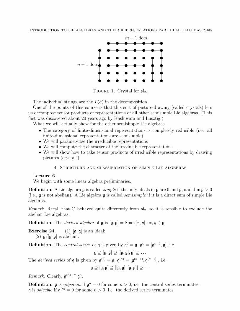
(5) The Clebsch-Gordan rule:
L(n)⊗ L(m) =n+m⊕
k=|n−m|k≡n−m mod 2
L(k).
There is a picture that goes with this rule (so you don’t actually need to rememberit):
INTRODUCTION TO LIE ALGEBRAS AND THEIR REPRESENTATIONS PART III MICHAELMAS 201015
m + 1 dots
n + 1 dots
Figure 1. Crystal for sl2.
The individual strings are the L(a) in the decomposition.One of the points of this course is that this sort of picture-drawing (called crystals) lets
us decompose tensor products of representations of all other semisimple Lie algebras. (Thisfact was discovered about 20 years ago by Kashiwara and Lusztig.)
What we will actually show for the other semisimple Lie algebras:
• The category of finite-dimensional representations is completely reducible (i.e. allfinite-dimensional representations are semisimple)• We will parameterise the irreducible representations• We will compute the character of the irreducible representations• We will show how to take tensor products of irreducible representations by drawing
pictures (crystals)
4. Structure and classification of simple Lie algebras
Lecture 6We begin with some linear algebra preliminaries.
Definition. A Lie algebra g is called simple if the only ideals in g are 0 and g, and dim g > 0(i.e., g is not abelian). A Lie algebra g is called semisimple if it is a direct sum of simple Liealgebras.
Remark. Recall that C behaved quite differently from sl2, so it is sensible to exclude theabelian Lie algebras.
Definition. The derived algebra of g is [g, g] = Span [x, y] : x, y ∈ g.
Exercise 24. (1) [g, g] is an ideal;(2) g/[g, g] is abelian.
Definition. The central series of g is given by g0 = g, gn = [gn−1, g], i.e.
g ⊇ [g, g] ⊇ [[g, g], g] ⊇ . . .
The derived series of g is given by g(0) = g, g(n) = [g(n−1), g(n−1)], i.e.
g ⊇ [g, g] ⊇ [[g, g], [g, g]] ⊇ . . .
Remark. Clearly, g(n) ⊆ gn.
Definition. g is nilpotent if gn = 0 for some n > 0, i.e. the central series terminates.g is solvable if g(n) = 0 for some n > 0, i.e. the derived series terminates.

16 IAN GROJNOWSKI
By the above remark, a nilpotent Lie algebra is necessarily solvable.
Remark. The term “solvable” comes from Galois theory (if the Galois group is solvable, theassociated polynomial is solvable by radicals). We will see shortly where the term “nilpotent”comes from.
Example 4.1. (1) n =
0 ∗ . . . ∗
0 . . . ∗. . .
...0
∈ gln the strictly upper triangular matrices
are a nilpotent Lie algebra.
(2) b =
∗ ∗ . . . ∗∗ . . . ∗
. . ....∗
∈ gln the upper triangular matrices are a solvable Lie algebra.
Exercise 25 (Essential). (a) Compute the central and derived series to check thatthese algebras are nilpotent and solvable respectively.
(b) Compute the center of these algebras.
(3) Let W be a symplectic vector space with inner product 〈, 〉 (recall that a symplecticvector space is equipped with a nondegenerate bilinear antisymmetric form, and thereis essentially one example: given a finite-dimensional vector space L let W = L + L∗
with inner product 〈L, L〉 = 〈L∗, L∗〉 = 0 and 〈v, v∗〉 = −〈v∗, v〉 = v∗(v)). Define theHeisenberg Lie algebra as
HW = W ⊕ Cc [w,w′] = 〈w,w′〉c, [c, w] = 0.
Exercise 26. Show this is a Lie algebra, and that it is nilpotent.
This is the most important nilpotent Lie algebra occurring in nature. For example,let L = C, then HW = Cp + Cq + Cc with [p, q] = c, [p, c] = [q, c] = 0 (as we knowfrom classifying the 3-dimensional Lie algebras!) Show that this has a representationon C[x] via q 7→ multiplication by x, p 7→ ∂/∂x, c 7→ 1.
(For a general vector space L, the basis vectors v1, . . . , vn map to multiplicationby x1, . . . , xn, and their duals map to ∂/∂x1, . . . , ∂/∂xn.)
Properties 4.1. (1) Subalgebras and quotients of solvable Lie algebras are solvable.Subalgebras and quotients of nilpotent Lie algebras are nilpotent.
(2) Let g be a Lie algebra, and let h be an ideal of g. Then g is solvable if and only if hand g/h are both solvable. (That is, solvable Lie algebras are built out of abelian Liealgebras, i.e. there is a refinement of the derived series such that the subquotientsare 1-dimensional and therefore abelian.)
(3) g is nilpotent iff the center of g is nonzero, and g/(center of g) is nilpotent.Indeed, if g is nilpotent, then the central series is
g ) g1 ) . . . ) gn−1 ) gn = 0,
and since gn = [gn−1, g] we must have gn−1 contained in the center of g.(4) g is nilpotent iff ad g ⊆ gl(g) is nilpotent, as we had an exact sequence
0→ center of g → g ad g→ 0.
INTRODUCTION TO LIE ALGEBRAS AND THEIR REPRESENTATIONS PART III MICHAELMAS 201017
Exercise 27. Prove the properties. (The proofs should all be easy and tedious.)
We now state a nontrivial result, which we will not prove.
Theorem 4.2 (Lie’s Theorem). Let g ⊆ gl(V ) be a solvable Lie algebra, and let the base fieldk be algebraically closed and have characteristic zero. Then there exists a basis v1, . . . , vn ofV with respect to which g ⊆ b(V ), i.e. the matrices of all elements of g are upper triangular.
Equivalently, there exists a linear function λ : g → k and an element v ∈ V , such thatxv = λ(x)v for all x ∈ g, i.e. v is a common eigenvector for all of g, i.e. a one-dimensionalsubrepresentation.
In particular, the only irreducible finite-dimensional representations of g are one-dimensional.
Exercise 28. Show that these are actually equivalent. (One direction should be obvious; inthe other, quotient by v1 and repeat.)
Exercise 29. Show that we need k to be algebraically closed.Show that we need k to have characteristic 0. [Hint: let g be the 3-dimensional Heisen-berg, and show that k[x]/xp is a finite-dimensional irreducible representation of dimensionmarkedly bigger than 1.]
Corollary 4.3. In characteristic 0, if g is a solvable finite-dimensional Lie algebra, then[g, g] is nilpotent.
Exercise 30. Find a counterexample in characteristic p.
Proof. Apply Lie’s theorem to the adjoint representation g → End (g). With respect tosome basis, ad g ⊆ b(g). Since [b, b] ⊆ n (note the diagonal entries cancel out when wetake the bracket), we see that [ad g, ad g] is nilpotent. Since ad [g, g] = [ad g, ad g] (it’s arepresentation!), we see that ad [g, g] is nilpotent, and therefore so is [g, g].
Theorem 4.4 (Engel’s Theorem). Let the base field k be arbitrary. g is nilpotent iff ad gconsists of nilpotent endomorphisms of g (i.e., for all x ∈ g, adx is nilpotent).
Equivalently, if V is a finite-dimensional representation of g such that all elements of gact on V by nilpotent endomorphisms, then there exists v ∈ V such that x(v) = 0 for allx ∈ g, i.e. V has the trivial representation as a subrep.
Equivalently, we can write x as a strictly upper triangular matrix.
Exercise 31. Show that these are actually equivalent.
Lecture 7
Definition. A symmetric bilinear form (, ) : g× g→ k is invariant if ([x, y], z) = (x, [y, z]).
Exercise 32. If a ⊆ g is an ideal and (, ) is an invariant bilinear form, then a⊥ is an ideal.
Definition. If V is a finite-dimensional representation of g, i.e. if ρ : g → gl(V ) is ahomomorphism, define the trace form to be (x, y)V = trace (ρ(x)ρ(y) : V → V ).
Exercise 33. Check that the trace form is symmetric, bilinear, and invariant. (They shouldall be obvious.)
Example 4.2. (, )ad is the “Killing form” (named after a person, not after an action). Thisis the trace form attached to the adjoint representation. That is, (x, y)ad = trace (ad x, ad y :g→ g).

18 IAN GROJNOWSKI
Theorem 4.5 (Cartan’s criteria). Let g ⊆ gl(V ) and let char k = 0. Then g is solvable ifand only if for every x ∈ g and y ∈ [g, g] the trace form (x, y)V = 0. (That is, [g, g] ⊆ g⊥.)
Exercise 34. Lie’s theorem gives us one direction. Indeed, if g is solvable then we can takea basis in which x is an upper triangular matrix, y is strictly upper triangular, and thenxy and yx both have zeros on the diagonal (and thus trace 0). That is, if g is solvable andnonabelian, all trace forms are degenerate. (The exercise is to convince yourself that this istrue.)
Corollary 4.6. g is solvable iff (g, [g, g])ad = 0.
Proof. If g is solvable, Lie’s theorem gives the trace to be zero. Conversely, Cartan’s criteriatell us that ad g = g/(center of g) is solvable, and therefore so is g.
Exercise 35. Not every invariant form is a trace form.Let H = C〈p, q, c, d〉 where [c, H] = 0, [p, q] = c, [d, p] = p, [d, q] = −q.
(1) Construct a nondegenerate invariant form on H.
(2) Show H is solvable.
(3) Extend the representation of 〈c, p, q〉 = H on k[x] to a representation of H.
Definition. The radical of g, R(g), is the maximal solvable ideal in g.
Exercise 36. (1) Show R(g) is the sum of all solvable ideals in g (i.e., show that thesum of solvable ideals is solvable).
(2) Show R(g/R(g)) = 0.
Theorem 4.7. In characteristic 0, the following are equivalent:
(1) g is semisimple(2) R(g) = 0(3) The Killing form (, )ad is nondegenerate (the Killing criterion).
Moreover, if g is semisimple, then every derivation D : g → g is inner, but not conversely(where we define the terms “derivation” and “inner” below).
Definition. A derivation D : g→ g is a linear map satisfying D[x, y] = [Dx, y] + [x, Dy].
Example 4.3. ad (x) is a derivation for any x. Derivations of the form ad (x) for some x ∈ gare called inner.
Remark. If g is any Lie algebra, we have the exact sequence
0→ R(g) → g g/R(g)→ 0
where R(g) is a solvable ideals, and g/R(g) is semisimple. That is, any Lie algebra hasa maximal semisimple quotient, and the kernel is a solvable ideal. This shows you howmuch nicer the theory of Lie algebras is than the corresponding theory for finite groups.In particular, the corresponding statement for finite groups is essentially equivalent to theclassification of the finite simple groups.
A theorem that we will neither prove nor use, but which is pretty:
Theorem 4.8 (Levi’s theorem). In characterstic 0, a stronger result is true. Namely, theexact sequence splits, i.e. there exists a subalgebra ß ⊆ g such that ß ∼= g/R(g). (Thissubalgebra is not canonical; in particular, it is not an ideal of g.) That is, g can be writtenas g = ß n R(g).
INTRODUCTION TO LIE ALGEBRAS AND THEIR REPRESENTATIONS PART III MICHAELMAS 201019
Exercise 37. Show that this fails in characteristic p. Let g = slp(Fp); show R(g) = FpI(note that the identity matrix in dimension p has trace 0), but that there is no complementto R(g) that is an algebra.
Proof of Theorem 4.7. First, notice that R(g) = 0 if and only if g has no nonzero abelianideals. (In one direction, an abelian ideal is solvable; in the other, notice that the last termof the derived series is abelian.)
From now on, (, ) refers to the Killing form (, )ad .(3) =⇒ (2): we show that if a is an abelian ideal of g, then a ⊆ g⊥. (Since the Killing
form is nondegenerate, this means a = 0, and therefore R(g) = 0.)Write g = a + h where h is a vector space complement to a (not necessarily an ideal). For
a ∈ a, ad a has block matrix
(0 ∗0 0
). For x ∈ g, ad x has block matrix
(∗ ∗0 ∗
). (This is
because a is an ideal, so [a, x] ∈ a for all x ∈ g, and moreover ad a acts by 0 on a.) Therefore,
trace (ad a · ad x) = trace (
(0 ∗0 0
)) = 0,
i.e. (a, g)ad = 0. Since the Killing form is nondegenerate, a = 0.(2) =⇒ (3): Let r ⊆ g⊥ be an ideal (e.g. r = g⊥), and suppose r 6= 0. Then r ⊆ gl(g) via
ad , and (x, y)ad = 0 for all x, y ∈ r. By Cartan’s criteria, ad r = r/(center of r) is solvable,so r is solvable, contradicting R(g) = 0.
Exercise 38. Show that R(g) ⊇ g⊥ ⊇ [R(g), R(g)].
(2),(3) =⇒ (1): Let (, )ad be nondegenerate, and let a ⊆ g be a minimal nonzero ideal.We claim that (, )ad |a is either 0 or nondegenerate.
Indeed, the kernel of (, )ad |a = x ∈ a : (x, a)ad = 0 = a ∩ a⊥ is an ideal!Cartan’s criteria imply that a is solvable if (, )ad |a is 0. Since R(g) = 0, we conclude that
(, )ad |a is nondegenerate.Therefore, g = a ⊕ a⊥, where a is a minimal ideal, i.e. simple. (Note that R(g) = 0 so a
cannot be abelian.)But now ideals of a⊥ are ideals of g, so we can apply the same argument to a⊥ since
R(g) = 0 =⇒ R(a⊥) = 0. Therefore, g = ⊕ai where the ai are simple Lie algebras.
Exercise 39. Show that if g is semisimple, then g is the direct sum of minimal ideals in aunique manner. That is, if g = ⊕ai where ai are minimal, and b is a minimal ideal of g,then in fact b = ai for some i. (Consider b ∩ aj.) Conclude that (1) =⇒ (2).
Lecture 8 Finally, we show that all derivations on semisimple Lie algebras are inner.Let g be a semisimple Lie algebra, and let D : g → g be a derivation. Cosnider the linearfunctional l : g → k via x 7→ trace (D · ad x). Since g is semisimple, the Killing form isa nondegenerate inner product giving an isomorphism with the dual, so ∃y ∈ g such thatl(x) = (y, x)ad . Our task is to show that D = ad y, i.e. that E := D − ad y = 0.
This is equivalent to showing that Ex = 0 for all x ∈ g, or equivalently that (Ex, z)ad = 0for all z ∈ g. Now,
ad (Ex) = E · ad x− ad x · E = [E, ad x] : g→ g
since ad (Ex)(z) = [Ex, z] = E[x, z]− [x, Ez]. Therefore,
(Ex, z)ad = trace g(ad (Ex) · ad z) = trace g([E, ad x] · ad z) = trace g(E, [ad x, ad z]).
20 IAN GROJNOWSKI
But by definition of E, trace g(E, ad a) = trace g(D, ad a)− (y, a)ad = 0.
Exercise 40. (1) A nilpotent Lie algebra always has non-inner derivations.(2) g = 〈a, b〉 with [a, b] = b only has inner derivations. Thus, this condition doesn’t
characterise semisimplicity.
Exercise 41. (1) Let g be a simple Lie algebra, (, )1 and (, )2 two non-degenerate invari-ant bilinear forms. Show ∃λ such that (, )1 = λ(, )2.
(2) Let g = slnC. We will shortly show that this is a simple Lie algebra. We have twonondegenerate bilinear forms: the Killing form (, )ad and (A, B) = trace (AB) in thestandard representation. Compute λ.
5. Structure theory
Definition. A torus t ⊆ g is an abelian subalgebra s.t. ∀t ∈ t the adjoint ad (t) : g → g isa diagonalisable linear map. A maximal torus is a torus that is not contained in any biggertorus.
Example 5.1. Let T = (S1)r ⊆ G where G is a compact Lie group (or T = (C×)r ⊆ Gwhere G is a reductive algebraic group). Then t = Lie (T ) ⊆ g = Lie (G) is a torus, maximalif T is. (This comes from knowing that representations of t are diagonalisable by an averagingargument, bur we don’t really know this.)
Exercise 42. (1) g = sln or g = gln, t the diagonal matrices (of trace 0 if inside sln) isa maximal torus.
(2)
(0 ∗0 0
)is not a torus. (We should know this is not diagonalisable!)
For a vector space V , let t1, . . . , tr : V → V be pairwise commuting diagonalisable linearmaps; let λ = (λ1, . . . , λr) ∈ Cn. Set Vλ = v ∈ V : tiv = λiv the simultaneous eigenspace.
Lemma 5.1. V =⊕
λ∈(C×)r Vλ.
Proof. Induct on r. For r = 1 follows from the requirement that t1 be diagonalisable.For r > 1, look at t1, . . . , tr−1 and decompose
V = ⊕V(λ1,...,λr−1).
Since tr commutes with t1, . . . , tr−1, it preserves the decomposition. Now decompose eachV(λ1,...,λr−1) into eigenspaces for tr.
Let t be the r-dimensional abelian Lie algebra with basis (t1, . . . , tr). The lemma assertsthat V is a semisimple (i.e. completely reducible) representation of t. V = ⊕Vλ is thedecomposition into isotypic representations. Namely, letting Cλ be the 1-dimensional repre-sentation wherein ti(w) = λiw, we have λ 6= µ =⇒ Cλ 6∼= Cµ, and Vλ is the direct sum ofdim Vλ copies of Cλ.
Exercise 43. Show that every irreducible representation of t is one-dimensional.
Another way of saying this is as follows. λ is a linear map t→ C, i.e. an element of the dualspace λ ∈ t∗ (sending λ(ti) = λi). Therefore, one-dimensional representations of t (which areall the irreducible representations of t) correspond to elements of t∗ = Homvector spaces(t, C).The decomposition
V = ⊕λ∈t∗Vλ, Vλ = v ∈ V : t(v) = λ(t)v

INTRODUCTION TO LIE ALGEBRAS AND THEIR REPRESENTATIONS PART III MICHAELMAS 201021
is called the weight space decomposition of V .Now, let g be a Lie algebra and t a maximal torus. The weight space decomposition of g
is
g = g0 ⊕⊕λ∈t∗λ6=0
gλ
where g0 = x ∈ g|[t, x] = 0 and gλ = x ∈ G : [t, x] = λ(t)x.
Definition. R = λ ∈ t∗|gλ 6= 0, λ 6= 0 is the set of roots of g.
We will now compute the root space decomposition for sln.
Example 5.2. g = sln, t = diagonal matrices in sln.
Let t =
t1 0. . .
0 tn
and Eij the matrix with 1 in the (i, j)th position and 0 elsewhere.
Then [t, Eij] = (ti − tj)Eij.Let εi ∈ t∗, εi(t) = ti. Then ε1, . . . , εn span t∗, but ε1 + . . . + εn = 0.
Remark. t is a subalgebra of Cn, so t∗ should be a quotient of (Cn)∗, and here is the relationby which it is a quotient.
Therefore, we can rewrite the above as [t, Eij] = (εi − εj)(t) · Eij.Therefore, the roots are R = εi − εj, i 6= j and g0 = t. (Note that we’ve shown t is a
maximal torus in the process.) The root space gεi−εj= CEij is one-dimensional.
That is, the root space decomposition of sln is:
sln = t⊕⊕
εi−εj∈R
gεi−εj
Exercise 44. “This is (a) an essential exercise, and (b) guaranteed to be on the exam. Thefirst should get you to do it, the second is irrelevant.”
Compute the root space decomposition for sln (as we just did), so2n, so2n+1, sp2n where tis the diagonal matrices in g, and we take the conjugate son defined by
son = A ∈ gln|JA + AT J = 0, J =
0 1
. . .. . .
1 0
(this is conjugate to the usual son since we’ve defined a nondegenerate inner product; in thisversion, the diagonal matrices are a maximal torus). The symplectic matrices are given bythe same embedding as before.
In particular, show that t is a maximal torus and the root spaces are one-dimensional.
Lecture 9 The Lie algebras we were working with last time are called the “classical” Liealgebras (they are automorphisms of vector spaces). The rest of the course will be concernedwith explaining how their roots control their representations.
Proposition 5.2. slnC is simple.

22 IAN GROJNOWSKI
Proof. Recall
slnC = t⊕⊕α∈R
gα
where R = εi − εj|i 6= j and gεi−εj= CEij.
Suppose r ⊆ sln is a nonzero ideal. Choose r ∈ r, r 6= 0, s.t. when we write r = t+∑
α∈R eα
with eα ∈ gα, the number of nonzero terms is minimal.First, suppose t 6= 0. Choose t0 ∈ t such that α(t0) 6= 0 for all α ∈ R (i.e., t0 has distinct
eigenvalues). Consider [t0, r] =∑
α∈r α(t0)eα. Note that this lies in r, and if it is nonzero, ithas fewer nonzero terms than r, a contradiction. Thus, [t0, r] = 0, i.e. r = t ∈ t.
Since t 6= 0, there exists α ∈ R with α(t) 6= 0 (i.e. it can’t have the same eigenvalue, sinceit’s trace 0). Then
[t, eα] = α(t)eα =⇒ eα ∈ r
Letting α = εi − εj, we have Eij ∈ r. Now,
[Eij, Ejk] = Eik for i 6= k [Esi, Eij] = Esj for s 6= j
and therefore Eab ∈ r for a 6= b. Finally,
[Ei,i+1, Ei+1,i] = Eii − Ei+1,i+1 ∈ r,
so in fact the entire basis for sln lies in r and r = sln.
Remark. This is actually a combinatorial statement about root spaces; we’ll see more aboutthis later.
That leaves us with the case t = 0. If r = cEij has only one nonzero term, we are doneexactly as above; therefore,
r = eα + eβ +∑
γ∈R−α,β
eγ, α 6= β
Choose t0 ∈ t such that α(t0) 6= β(t0); then some linear combination of [t0, r] and r will havefewer nonzero terms than r, a contradiction.
Proposition 5.3. Let g be a semisimple Lie algebra. Then maximal tori exist (i.e. arenonzero). Moreover, g0 = x ∈ g|[t, x] = 0 = t. (Recall that t is not defined to bethe maximal abelian subalgebra, but as the maximal abelian subalgebra whose adjoint actssemisimply.)
We won’t prove this; the proof involves introducing the Cartan subalgebra and showingthat it’s the same as a maximal torus. As a result, we will sometimes be calling t the Cartansubalgebra.
This means that the root space decomposition of a semisimple Lie algebra is
g = t⊕⊕α∈R
gα
as we have, of course, already seen for the classical Lie algebras.
Theorem 5.4 (Structure theorem for semisimple Lie algebras, part I). Let g be a semisimpleLie algebra over C, and let t ⊆ g be a maximal torus. Write g = t⊕
⊕α∈R gα. Then
(1) CR = t∗, i.e. the roots span t∗.(2) dim gα = 1.

INTRODUCTION TO LIE ALGEBRAS AND THEIR REPRESENTATIONS PART III MICHAELMAS 201023
(3) If α, β ∈ R and α + β ∈ R then [gα, gβ] = gα+β. If α + β 6∈ R and α 6= −β then[gα, gβ] = 0.
(4) [gα, g−α] ⊆ t is one-dimensional, and gα ⊕ [gα, g−α] ⊕ g−α is a Lie subalgebra of gisomorphic to sl2. (In particular, α ∈ R =⇒ −α ∈ R.
Exercise 45. Check this for the classical Lie algebras.
Proof. (1) Suppose not, then there exists t ∈ t such that α(t) = 0 for all α ∈ R. Butthen [t, gα] = 0; as [t, t] = 0 by definition, we see that t is central in g. However, g issemisimple, so it has no abelian ideals, in particular no center.
We will now show a sequence of statements.(a) [gλ, gµ] ⊆ gλ+µ if λ, µ ∈ t∗.
Indeed, for x ∈ gλ and y ∈ gµ we have
[t, [x, y]] = [[t, x], y] + [x, [t, y]] = (λ(t) + µ(t))[x, y].
This shows that [gα, gβ] ⊆ gα+β if α+β ∈ R, is 0 if α+β 6∈ R, and [gα, g−α] ⊆ t.(b) (gλ, gµ)ad = 0 if λ 6= −µ; (, )ad |gλ⊕g−λ
is nondegenerate.
Proof. Let x ∈ gλ and y ∈ gµ. Recall (x, y)ad = trace g(ad x · ad y). To showthat it’s zero, we show that ad x · ad y is nilpotent.Indeed, (ad x · ad y)Ngα ⊆ gα+N(λ+µ), so if λ 6= −µ then for N 0 this is zero.On the other hand, (, )ad is nondegenerate and g = ⊕λ∈t∗gλ⊕g−λ, so (, )ad |gλ⊕g−λ
must be nondegenerate.
(c) In particular, (, )ad |t is nondegenerate, as t = g0.
Remark. (, )ad |t 6= (, )ad t (which is zero since t is abelian).
Therefore, the Killing form defines an isomorphism ν : t → t∗ with ν(t)(t′) =(t, t′)ad . It also defines an induced inner product (well, symmetric bilinear formto be precise – we don’t know it’s positive) on t∗, via (ν(t), ν(t′)) = (t, t′)ad .
(d) α ∈ R =⇒ −α ∈ R, since (, )ad is nondegenerate on gα⊕g−α, but (gα, gα)ad = 0if α 6= 0. In particular, g−α
∼= g∗α via the Killing form.(e) x ∈ gα, y ∈ g−α =⇒ [x, y] = (x, y)ad ν−1(α).
Proof.(t, [x, y])ad = ([t, x], y)ad = α(t)(x, y)ad ,
which is exactly what we want.
(f) Let eα ∈ gα be nonzero, and pick e−α ∈ g−α such that (eα, e−α)ad 6= 0. Then[eα, e−α] = (eα, e−α)ad ν−1(α). To show that eα, e−α, and their bracket give acopy of sl2, we need to compute
[ν−1(α), eα] = α(ν−1(α))eα = (α, α)eα
We will be done if we show that (α, α) 6= 0 (then we get a copy of sl2 afterrenormalising).
Proposition 5.5. (α, α) 6= 0 for all α ∈ R.
Proof. Next time.

24 IAN GROJNOWSKI
Lecture 10 We now prove the last proposition, (α, α) 6= 0 for all α ∈ R.
Proof. Suppose otherwise. Let mα = 〈eα, e−α, ν−1(α)〉. If (α, α) = 0, i.e. if [ν−1(α), eα] = 0,then [mα, mα] = Cν−1α and mα is solvable. However, by Lie’s theorem this implies thatad [mα, mα] acts by nilpotents on g, i.e. ad ν−1(α) is nilpotent. Since ν−1(α) ∈ t, it is alsodiagonalisable, and the only diagonalisable nilpotent element is 0. However, α ∈ R =⇒α 6= 0.
Now, define
hα =2
(α, α)ν−1(α)
and rescale e−α such that (eα, e−α)ad = 2/(α, α).
Exercise 46. The map (eα, hα, e−α) 7→ (e, h, f) gives an isomorphism mα∼= sl2.
Remark. In sln, the root spaces are spanned by Eij, so we are saying that the subalgebra ofmatrices of the form
a ∗
∗ −a
is a copy of sl2, which is obvious. The cool thing is that something like this happens for allthe semisimple Lie algebras, and that this lets us know just about everything about them.
We will now use our knowledge of the representation theory of sl2. We show
Claim. dim g−α = 1 for all α ∈ R.
Proof. Pick a copy of mα = 〈eα, hα, e−α〉 ∼= sl2. Suppose dim g−α > 1, then the mapg−α → Cν−1(α), x 7→ [eα, x] has a kernel. That is, there is a v ∈ g−α such that ad eα · v = 0.Then v is a highest-weight vector (it comes from a root space g−α, so it’s an eigenvector ofad hα), and its weight is determined by
ad hα · v = −α(hα)v = −2v.
That is, v is a highest-weight vector of weight −2. However, we know that in finite-dimensional representations of sl2 (which g is, since gα acts on it) the highest weights arenonnegative integers. This contradiction shows the claim.
Before we finish proving the theorem we had (we still need to show [gα, gβ] = gα+β whenα, β, α + β ∈ R), we show further combinatorial properties of the roots.
Theorem 5.6 (Structure theorem, continued). (1)
2(α, β)
(α, α)∈ Z for all α, β ∈ R
(2) If α ∈ R and kα ∈ R, then k = ±1.

INTRODUCTION TO LIE ALGEBRAS AND THEIR REPRESENTATIONS PART III MICHAELMAS 201025
(3) ⊕k∈Z
gβ+αk
is an irreducible module for (sl2)α = 〈eα, hα, e−α〉. In particular,
kα + β|kα + β ∈ R, k ∈ Z ∪ 0
is of the form β−pα, β−(p−1)α, . . . , β, . . . , β +(q−1)α, β +qα where p−q = 2(α,β)(α,α)
.
We call this set the “α string through β”.
(1): let q = maxk : β + kα ∈ R and let v ∈ gβ+qα be nonzero. Then ad eα · v ∈gβ+(q+1)α = 0, and
ad hα · v = (β + qα)(hα) · v =
(2(β, α)
(α, α)+ 2q
)v.
That is, v is a highest weight vector for (sl2)α with weight 2(β, α)/(α, α) + 2q. Since theweight in a finite-dimensional representation is an integer, we see that 2(β, α)/(α, α) ∈ Z.
Proof. (3): Structure of sl2-modules tells us that (ad e−α)rv 6= 0 for 0 ≤ r ≤ 2(α,β)(α,α)
+2q = N ,
and that (ad eα)N+1v = 0. Therefore, β + qα − kα, 0 ≤ k ≤ N are all roots (or possiblyequal to zero – in any case, they have nonzero root space). This certainly is an irreducible(sl2)α module; we now need to show that there are no other roots in the α string through β.We do this by repeating the same construction from the bottom up:
Let p = maxk : β − kα ∈ r and let w ∈ gβ−pα be nonzero. then ad e−α · w = 0 andad hα ·w = (2(β, α)/(α, α)−2p)w, so w is a lowest-weight vector of weight 2(β, α)/(α, α)−2p.By applying ad eα repeatedly, we get an irreducible sl2 module with roots β − pα, β − (p−1)α, . . . , β + (p− 2(α, β)/(α, α))α.
Now by construction we have p−2(α, β)/(α, α) ≤ q and also q+2(α, β)/(α, α) ≤ p, whichmeans that in fact p− q = 2(α, β)/(α, α) and the two submodules we get coincide.
(2): By (1) we have 2(α, kα)/(kα, kα) = 2/k ∈ Z and 2(kα, α)/(α, α) = 2k ∈ Z. Thus, itsuffices to show that α ∈ R =⇒ 2α 6∈ R.
But indeed, suppose 2α ∈ R and let v ∈ g−2α be nonzero. Then [eα, v] ∈ g−α has theproperty that
([eα, v], eα) = (v, [eα, eα]) = 0,
and since gα is one-dimensional and spanned by eα, we find ([eα, v], gα) = 0. Since (, )|gα⊕g−α
is nondegenerate, this means [eα, v] = 0, i.e. v ∈ g−2α is a highest-weight vector for (sl2)α
with highest weight −4. This doesn’t happen in finite-dimensional representations, so g−2α =0 and 2α is not a root.
(In fact, we could derive this from (3), since we know that there is a 3-dimensional sl2-module running through 0.)
We finally show [gα, gβ] = gα+β when α, β, α + β ∈ R. Indeed, we have just shownthat ⊕gβ+kα is an irreducible representation of mα, and ad eα : gβ+kα → gβ+(k+1)α is anisomorphism for k < q. Since q ≥ 1, we see that ad eα · gβ = gα+β.
Remark. The combinatorial statement of (3) is rather clunky. We now “unclunk” it:
For α ∈ t∗, define sα : t∗ → t∗ by sα(v) = v − 2(α,v)(α,α)
α (a reflection of v about α).
Claim. (3) implies (and in fact, is equivalent to) sα(β) ∈ R whenever α, β ∈ R.
26 IAN GROJNOWSKI
Proof. Let r = 2(α, β)/(α, α). If r ≥ 0, then p = q + r ≥ r; if r ≤ 0 then q = p − r ≥ −r.Either way, β − rα is in the α string through β.
Over the next several lectures, we will classify the root systems as combinatorial objects.Before we do that, we state some further properties of the roots:
Proposition 5.7. (1) α, β ∈ R =⇒ (α, β) ∈ Q.(2) If we pick a basis β1, . . . , βl of t∗, with βi ∈ R, then any β ∈ R expands as
∑qiβi
with qi ∈ Q, i.e. dim QR = dimC t.(3) (, ) is positive definite on QR.
Lecture 11
Proof of the Proposition at the end of last lecture. (1) It suffices to show (β, β) ∈ Q forall β ∈ R.
Let h, h′ ∈ t, then
(h, h′)ad = trace g(ad had h′) =∑α∈R
α(h)α(h′)
since g = t +⊕
α∈R gα by the structure theorem.Therefore, for λ, µ ∈ t∗,
(λ, µ) = (ν−1(λ), ν−1(µ))ad =∑α∈R
α(ν−1λ)α(ν−1µ) =∑α∈R
(λ, α)(µ, α).
In particular, (β, β) =∑
α∈R(α, β)2. Multiplying by 4/(β, β)2, we get
4
(β, β)=
∑α∈R
(2(α, β)
(β, β)
)2
∈ Z
and therefore (β, β) ∈ Q.(2) Let B be the Gram matrix of the basis, Bij = (βi, βj).
Exercise 47. (, ) is a nondegenerate symmetric bilinear form =⇒ det B 6= 0.
Let β =∑
ciβi ∈ R. Then (β, βi) =∑
cj(βi, βj). Therefore, we can recover thevector of ci as
(c1, . . . , cl) = ((β, β1), . . . , (β, βl))(BT )−1
Since the inner products of roots are all rational, we see that ci ∈ Q as well.(3) Let λ ∈ QR. Then λ =
∑ciβi with ci ∈ Q, and (λ, α) ∈ Q for all α ∈ R. Moreover,
(λ, λ) =∑
α∈R(λ, α)2 ≥ 0, and if (λ, λ) = 0 then (λ, α) = 0 for all α ∈ R. Since Rspans t∗ and (, ) is nondegenerate, this implies that λ = 0.
6. Root systems
Let V be a vector space over R, (, ) an inner-product (i.e. a positive-definite symmetricbilinear form). For α ∈ V , α 6= 0, write α∨ = 2α
(α,α), so that (α, α∨) = 2.
Define sα : V → V by sα(v) = v − (v, α∨)α.
INTRODUCTION TO LIE ALGEBRAS AND THEIR REPRESENTATIONS PART III MICHAELMAS 201027
Lemma 6.1. sα is the reflection in the hyperplane orthogonal to α. In particular, all butone of the eigenvalues of sα are 1, and the remaining one is −1 (with eigenvector α). Thus,s2
α = 1, or (sα + 1)(sα − 1) = 0, and sα ∈ O(V, (, )), the orthogonal group of V defined bythe inner product (, ).
Proof. Write V = Rα⊕ α⊥. Then sα(α) = α− (α, α∨)α = −α, and sα fixes all v ∈ α⊥.
Definition. A root system R in V is a finite set R ⊆ V such that
(1) 0 6∈ R, RR = V
(2) For all α, β ∈ R, the inner product (α, β∨) ∈ Z.(3) For all α ∈ R, sα(R) ⊆ R. (In particular, sα(α) = −α ∈ R.)
Moreover, R is called reduced if(4) α, kα ∈ R =⇒ k = ±1.
Example 6.1. Let g be a semisimple Lie algebra, g = t +⊕
α∈R gα. Then R ⊆ RR is areduced root system.
Definition. Let W ⊆ GL(V ) be the group generated by reflections sα, α ∈ R; W is calledthe Weyl group of R.
Observe that |W | < ∞: W acts on R by permutations, and since 0 6∈ R, the action isfaithful (since sα ∈ W for all α ∈ R and sα sends α to −α, the only possible W -invariantelement is 0, but it is not in R). Thus, W injects into Sym(R), so |R| <∞ =⇒ |W | <∞.
Definition. The rank of R is the dimension of V .
Definition. An isomorphism of root systems (R, V )→ (R′, V ′) is a linear bijection φ : V →V ′ such that φ(R) = R′. Note that φ is not required to be an isometry.
Definition. If (R, V ) and (R′, V ′) are root systems, so is their direct sum (R tR′, V ⊕ V ′).A root system which is not isomorphic to a direct sum is called irreducible.
Example 6.2. (1) Rank 1: V = R, (x, y) = xy. R = α,−α with α 6= 0. W = Z/2.
−α← • → α
Exercise 48. This is the only rank 1 root system.
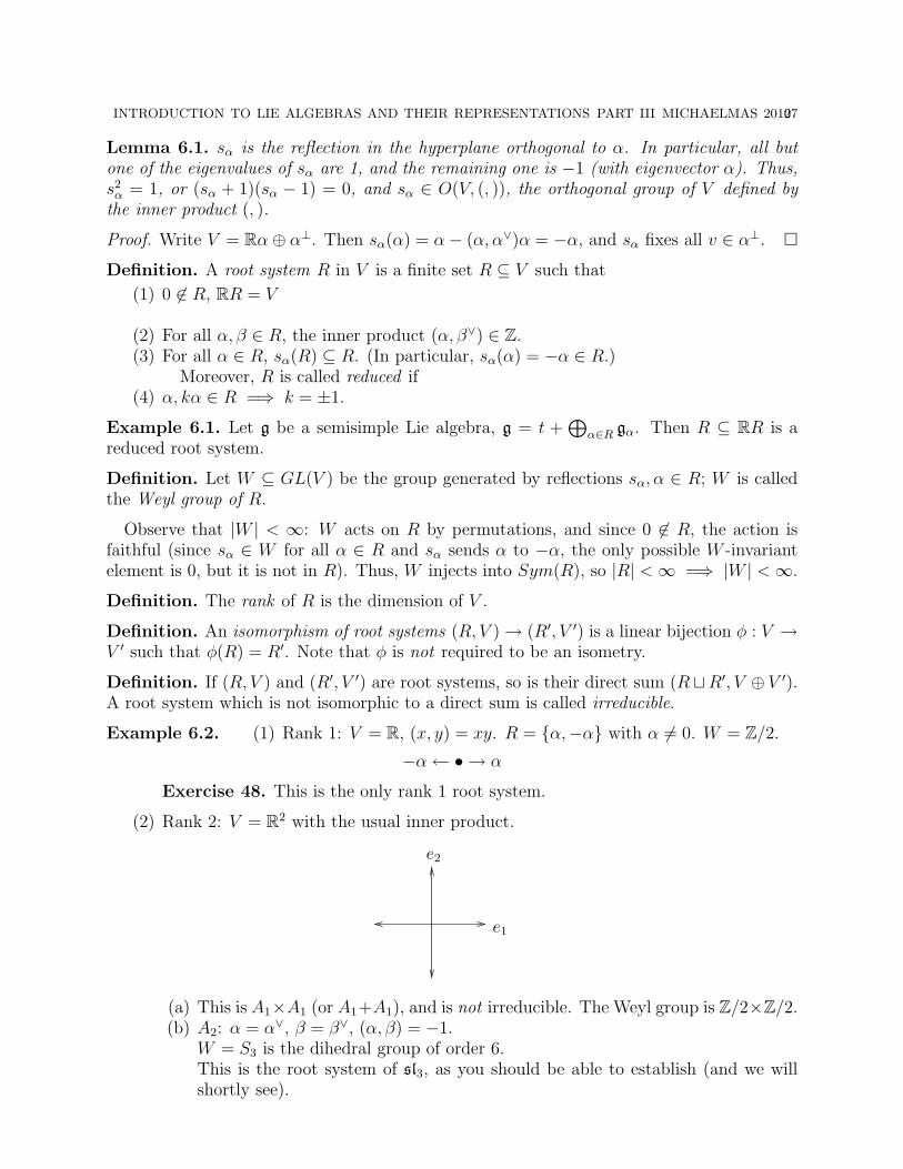
(2) Rank 2: V = R2 with the usual inner product.
e2
e1
(a) This is A1×A1 (or A1+A1), and is not irreducible. The Weyl group is Z/2×Z/2.(b) A2: α = α∨, β = β∨, (α, β) = −1.
W = S3 is the dihedral group of order 6.This is the root system of sl3, as you should be able to establish (and we willshortly see).

28 IAN GROJNOWSKI
α
β
β β + α β + 2α
α
(c) B2: α = e1, β = e2− e1: (α, α) = 1 and (β, β) = 2. α and α + β are short roots;β and 2α + β are long roots.W is the dihedral group of order 8.This is the root system of sp4 and so5.
(d) G2:At this point, we clearly should look at all the dihedral groups, right? Unfor-tunately, no: the condition (α, β∨) ∈ Z rules out all but the dihedral group oforder 12. This is the root system of a Lie group, but not one of the classical
α
β
ones (symmetries of octonions).
Exercise 49. All of these are indeed root systems. They are the only rank 2 root systems,and A2, B2, and G2 are irreducible.
Lemma 6.2. If R is a root system, so is R∨ = α∨|α ∈ R.
Exercise 50. Prove it.
Definition. R is simply laced if all the roots have the same length.
Exercise 51. If R is simply laced, then (R, V ) ∼= (R′, V ′) where (α, α) = 2 for all α ∈ R′
(i.e. α = α∨). [Hint: If irreducible, rescale; if not, break up into a direct sum of irreducibles.]
We would like to look at roots as coming from a lattice. We will see why length-2 is souseful.
Definition. A lattice L is a finitely-generated free abelian group (∼= Zl for some l) withbilinear form L⊕ L→ Z, such that (L⊗Z R, (, )) is an inner product space.A root of L is α ∈ L such that (α, α) = 2. We write RL = l ∈ L|(l, l) = 2 for the roots ofL.

INTRODUCTION TO LIE ALGEBRAS AND THEIR REPRESENTATIONS PART III MICHAELMAS 201029
Note that α ∈ RL =⇒ sα(L) ⊆ L.
Lemma 6.3. RL is a simply laced root system in RRL.
Proof. The only non-obvious claim is |RL| <∞. However, RL is the intersection of a compactset (sphere of radius
√2) with a discrete set (the lattice), so is finite.
Definition. We say that L is generated by roots if ZRL = L. Note that then L is an evenlattice, i.e. (l, l) ∈ 2Z for all l ∈ L.
Example 6.3. L = Zα with (α, α) = λ. If λ = 2 then RL = ±α and L = ZRL; if k2λ26= 1
for all k then RL = ∅.
We now characterise the simply laced root systems.
(1) An. Consider Zn+1 =⊕n+1
i=1 Zei with (ei, ej) = δij (the square lattice). Define
L = l ∈ Zn+1|(l, e1 + . . . + en) = 0 = aiei|∑
ai = 0 ∼= Zn.
Then RL = ei − ej|i 6= j, #RL = n(n + 1), ZRL = L.If α = ei − ej then sα applied to a vector with coordinates x1, . . . , xn+1 (in basis
e1, . . . , en+1) swaps the i and j coordinate; therefore, W = 〈sei−ej〉 = Sn+1.
(RL, RL) is the root system of type An. Note that n is the rank of the root system,not the index of the associated Lie algebra.
Exercise 52. (a) “You should not believe a word I say”: Check these statements!(b) Draw L ⊆ Zn+1 and RL for n = 1, 2. Check that A1 and A2 agree with the
previous pictures.(c) Show that the root system of sln+1 has type An.
(2) Dn. Consider the square lattice Zn. The roots are RZn = ±ei ± ej|i 6= j. Set
L = ZRL = l =∑
aiei|ai ∈ Z,∑
ai even
sei−ejswaps the ith and jth coordinate as before; sei+ej
flips the sign of both the ithand the jth coordinate.
(RL, ZRL) is called Dn; #RL = 2n(n− 1). The Weyl group is
W = (Z/2)n−1 o Sn
where (Z/2)n−1 is the subgroup of even number of sign changes. (Possibly I mean(Z/2)n−1 n Sn.)
Exercise 53. (a) Check these statements!(b) Dn is irreducible if n ≥ 3.(c) RD3 = RA3 , RD2 = RA1 ×RA1
(d) The root system of so2n has type Dn.
Lecture 12 We continue our classification of the simply laced root systems:
(1) E8. Let
Γn = (k1, . . . , kn)|either all ki ∈ Z or all ki ∈ Z +1
2and
∑ki ∈ 2Z.
Consider α = (12, 1
2, . . . , 1
2) ∈ Γn, and note that (α, α) = n/4. Thus, if Γn is an even
lattice, we must have 8|n.
30 IAN GROJNOWSKI
Exercise 54. (a) Γ8n is a lattice.(b) For n > 1 the roots of Γ8n are a root system of type Dn
(c) The roots in Γ8 are ±ei±ej, i 6= j; 12(±e1±e2±. . .±e8), with an even number of − signs.
The root system of Γ8 is called the root system of type E8. The number of roots is
#RΓ8 =
(8
2
)· 4 + 128 = 240.
To check that you’re awake, the dimension of the associated Lie algebra is 280 +rank(RΓ8) = 248.
Remark. E8 is weird. Its smallest representation is the adjoint representation ofdimension 248. This is quite unlike son, sln, etc., which had dimension O(n2) andan n-dimensional representation. There isn’t a good understanding of why E8 is likethat.
Exercise 55. Can you compute #W , the order of the Weyl group of E8? [Answer:214 · 35 · 52 · 7]
Exercise 56. If R is a root system and α ∈ R, then α⊥ ∩R is a root system.
We will now apply this to Γ8. Let α = 12(1, 1, . . . , 1) and β = e7 + e8.
(2)
Definition. α⊥ ∩RΓ8 is a root system of type E7.〈α, β〉⊥ ∩RΓ8 is a root system of type E6.
Exercise 57. Show #RE7 = 126 and #RE6 = 72. Describe the corresponding rootlattices.
Remark. These lattices are reasonably natural objects. Indeed, if we took the as-sociated algebraic group and its maximal torus, there is a natural lattice associatedwith it coming from the fundamental group. Equivalently, we can think of the grouphomomorphisms to (or from) C×. This isn’t quite the root lattice, but it’s closelyrelated (and we might say more about it later).
Theorem 6.4. (1) (“ADE classification”) The complete list of irreducible simply lacedroot systems is
An, n ≥ 1, Dn, n ≥ 4, E6, E7, E8.
No two root systems in this list are isomorphic.(2) The remaining irreducible reduced root systems are denoted by
B2 = C2, Bn, Cn, n ≥ 3, F4, G2
where
RBn = ±ei,±ei ± ej, i 6= j ⊆ Zn
RCn = ±2ei,±ei ± ej, i 6= j ⊆ Zn
with R∨Cn= RBn. The root system of type Bn corresponds to so2n+1, and the root
system of type Cn corresponds to sp2n. The Weyl groups are
WBn = WCn = (Z/2)n o Sn.

INTRODUCTION TO LIE ALGEBRAS AND THEIR REPRESENTATIONS PART III MICHAELMAS 201031
The root system F4 is defined as follows: let Q = (k1, . . . , k4)|all ki ∈ Z or all ki ∈ Z + 12
and take
RF4 = α ∈ Q|(α, α) = 2 or (α, α) = 1 = ±ei,±ei ± ej, i 6= j,1
2(±e1 ± . . .± e4).
Remark. The duality between RBn and RCn suggests some form of duality between so2n+1
and sp2n. We will see it later.
To prove this theorem, we will first choose a good basis for V (the space spanned by theroot lattice). Choose f : V → R linear such that f(α) 6= 0 for all α ∈ R.
Definition. A root α ∈ R is positive, α ∈ R+, if f(α) > 0.A root α ∈ R is negative, α ∈ R−, if f(α) < 0. (Equivalently, −α ∈ R+.)A root α ∈ R+ is simple, α ∈ Π, if α is not the sum of two positive roots.
Example 6.4. (1) An: the roots are R = ei − ej|i 6= j. Choose
f(e1) = n + 1, f(e2) = n, . . . , f(en+1) = 1.
Then R+ = ei − ej|i < j.Since f(R) ∈ Z, if f(α) = 1 then α must be simple. Therefore, Π ⊇ e1 −
e2, . . . , en − en+1. On the other hand, it is clear that the positive integer span ofthese is R+, so in fact we have equality.
(2) Bn: R = ±ei,±ei ± ej, i 6= j. Take f(e1) = n, . . . , f(en) = 1. Then R+ =ei, ei ± ej|i < j and Π = e1 − e2, . . . , en−1 − en, en.
(3) Cn: R = ±2ei,±ei±ej, i 6= j. R+ = 2ei, ei±ej, i < j and Π = e1−e2, . . . , en−1−en, 2en.
(4) Dn: R = ±ei ± ej, i 6= j, Π = e1 − e2, . . . , en−1 − en, en−1 + en.(5) E8: set f(e1) = 28 = 1 + 2 + . . . + 7, and f(ei) = 9− i for i = 2 . . . 8. Then
R+ = ei ± ej, i < j,1
2(e1 ± e2 ± . . .± e8) with an even number of − signs
and
Π = e2 − e3, . . . , e7 − e8︸ ︷︷ ︸f=1
,1
2(e1 + e8 − e2 − . . .− e7)︸ ︷︷ ︸
f=2
, e7 + e8︸ ︷︷ ︸f=3
Exercise 58. Check all of these (by finding a suitable function f where one is not listed).Also find the simple roots for E6, E7, F4, and G2.
Remark. So far we have made two choices. We have chosen a maximal torus, and we havechosen a function f . Neither of these matters. We may or may not prove this about themaximal torus later; as for f , note that the space of functionals f is partitioned into cellswithin which we get the same notions of positive roots. The Weyl group acts transitively onthese cells, which should show that the choice of f does not affect the structure of the rootsystem we are deriving
Proposition 6.5. (1) α, β ∈ Π =⇒ α− β 6∈ R.(2) α, β ∈ Π, α 6= β =⇒ (α, β∨) ≤ 0 (i.e. the angle between α and β is obtuse).(3) Every α ∈ R+ can be written as α =
∑kiαi with αi ∈ Π and ki ∈ Z≥0.
(4) Simple roots are linearly independent.(5) α ∈ R+, α 6∈ Π =⇒ ∃αi ∈ Π such that α− αi ∈ R+.
32 IAN GROJNOWSKI
(6) R is irreducible iff Π is indecomposable (i.e. Π 6= Π1 t Π2 with (Π1, Π2) = 0).
Exercise 59. Prove this! (Either by a case-by-case analysis – which you should do in a fewcases anyway – or by finding a uniform proof from the axioms of a root system.)
We will now find another way to represent the root system. Let Π = α1, . . . , αl, letaij = (α∨i , αj).
Definition. A = (aij) is the Cartan matrix.
Properties 6.6. (1) aij ∈ Z, aii = 2, aij ≤ 0 for i 6= j(2) aij = 0⇔ aji = 0(3) det A > 0(4) All principal subminors of A have positive determinant.
Proof. The first two should be obvious from the above. To prove the determinant, note that
A =
2
(α1,α1)0
. . .
0 2(αl,αl)
· ((αi, αj))
The first matrix is diagonal with positive entries, the second one is the Gram matrix of apositive definite bilinear form and so has positive determinant.
The last property follows because any principal subminor of A (i.e. obtained by removingthe same set of rows and columns) has the same form as A.
We will represent A by a Dynkin diagram. The vertices correspond to simple roots.Between vertices αi and αj there are aijaji lines (note that this value can be 0 or 1 in thesimply laced diagrams, may be 2 in Bn or Cn, and may be 3 in G2). If there are 2 or 3 lines,we put an arrow towards the short root.
Exercise 60. Show the Dynkin diagrams are as we claim.
Lecture 13
Exercise 61. If (R, V ) is an irreducible root system with positive roots R+, then there is aunique root θ ∈ R+ such that ∀α ∈ Π, θ + α 6∈ R+. This is called the highest root.
At the moment, the easiest way to prove this is to examine all the root systems wehave. Later we’ll give a uniform proof (and show the relationship between θ and the adjointrepresentation).
Example 6.5. In An, the highest root is e1 − en+1.
Define the “extended Cartan matrix” A by setting α0 = −θ (and then A = (aij)0≤i,j≤l
with aij = (α∨i , αj) =2(αi,αj)
(αi,αi)).
The associated diagram is called the “extended” or “affine” Dynkin diagram.
Example 6.6. A1 has A = (2) and A =
(2 −2−2 2
).
INTRODUCTION TO LIE ALGEBRAS AND THEIR REPRESENTATIONS PART III MICHAELMAS 201033
e1 − e2
e2 − e3
e3 − e4
en − en+1
An
e1 − e2
e2 − e3
e3 − e4
en−1 − en
en−1 + enDn
E8
E7
E6
Bn
en−1 − en
en
en−1 − en
2enCn
G2
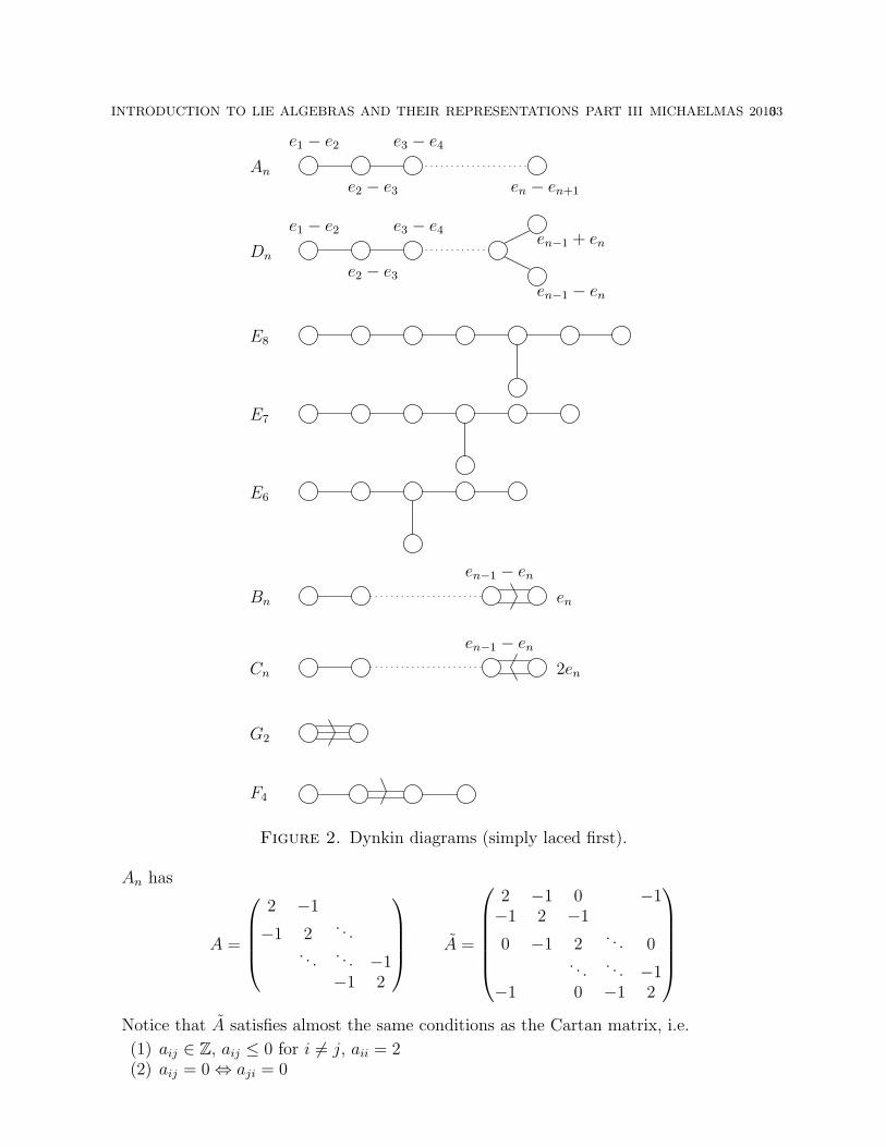
F4
Figure 2. Dynkin diagrams (simply laced first).
An has
A =
2 −1
−1 2. . .
. . . . . . −1−1 2
A =
2 −1 0 −1−1 2 −1
0 −1 2. . . 0
. . . . . . −1−1 0 −1 2
Notice that A satisfies almost the same conditions as the Cartan matrix, i.e.
(1) aij ∈ Z, aij ≤ 0 for i 6= j, aii = 2(2) aij = 0⇔ aji = 0

34 IAN GROJNOWSKI
(3) det A = 0, and every principal subminor of A has positive determinant.
The third property follows since A is related to the Gram matrix for α0, . . . , αl, which arenot linearly independent.
Exercise 62. Write down A and the extended Dynkin diagram for all types. To get youstarted, in Bn we have α0 = −e1 − e2, in Cn we have α0 = −2e1, and in Dn we haveα0 = −e1 − e2.
Exercise 63. Show that A(2)n (“twisted An”) also has determinant 0. (See Figure 3.)
Exercise 64. The Dynkin diagram of AT is the Dynkin diagram of A with the arrowsreversed.
These diagrams (plus their transposes) are (almost) all the non-garbage Lie algebras outthere. (We’ll be slightly more precise about the meaning of “non-garbage” later.)
Theorem 6.7. An irreducible (i.e., connected) Dynkin diagram is one of An, Bn, Cn, Dn,E6, E7, E8, F4, and G2.
Proof. (1) First, we classify the rank-2 Dynkin diagrams, i.e. their Cartan matrices:
A =
(2 −a−b 2
)with det A = 4−ab > 0. This leaves the options (a, b) = (0, 0) (A1×A1), (1, 1) (A2),(2, 1) or (1, 2) (B2), and (3, 1) or (1, 3) (G2).
(2) Observe any subdiagram of a Dynkin diagram is a Dynkin diagram. In particular,since the affine Dynkin diagrams have determinant 0, they are not subdiagrams of aDynkin diagram.
(3) A Dynkin diagram contains no cycles. Indeed, let α1, . . . , αn be distinct simple roots,
and consider α =∑
αi/√
(αi, αi). Then
0 < (α, α) = n +∑i<j
2(αi, αj)√(αi, αi)(αj, αj)
= n−∑i<j
√aijaji.
Therefore,∑
i<j
√aijaji < n. On the other hand, if we had a cycle on n simple roots,
it would have at least n edges, giving∑
i<j
√aijaji ≥ n, a contradiction.
(4) If a diagram is simply laced, it is A, D, or E:Suppose it’s not of type A. Since D4 is not a subdiagram, any branchings are at
most 3-way; and since Dn is not a subdiagram for n > 4, there is exactly one branchpoint. Therefore, the diagram is T-shaped, with p, q, and r vertices in each leg. Wecall this shape Tp,q,r; e.g., E8 = T5,3,2.
Exercise 65. Finish the proof in one of two ways:(a) By using the fact that E6, E7, E8 are not subdiagrams of a Dynkin diagram; or(b) By showing det Tp,q,r = pq + pr + qr− pqr, and concluding that Dn, E6, E7, and
E8 are the only possibilities. (E.g.: det E8 = 15 + 10 + 6− 30 = 1.)
(5) We now deal with the non-simply-laced diagrams.
Exercise 66. If there is a triple bond in the diagram, then the Dynkin diagram isG2. (Note that we took care of one of the possibilities in G2; you need to check thepossibility of a double and a triple bond, and of two triple bonds.)

INTRODUCTION TO LIE ALGEBRAS AND THEIR REPRESENTATIONS PART III MICHAELMAS 201035
An
Dn
E8
E7
E6
Bn
Cn
G2
F4
An(2)
Figure 3. Affine Dynkin diagrams.
Finally, if there is a double bond in the diagram, then by Cn and A(2)n there’s only
one of them, and the diagram does not branch by Bn. If the double bond is in themiddle, we have F4 (since we don’t have F4); otherwise, we have Bn or Cn.
36 IAN GROJNOWSKI
Exercise 67. Compute the determinant of all the Cartan matrices.
Example 6.7.
A1 : det(2) = 2 A2 : det
(2 −1−1 2
)= 3 A3 : det = 4 . . .
This comes out of the following: SLn+1 = X : det X = 1 has center consisting of (n+1)throots of unity (i.e. a cyclic group of order n + 1). Note that the order of the center is equalto the determinant of the Cartan matrix. This is true in general: the order of the center ofa simply connected algebraic group with Lie algebra g and associated Cartan matrix A isequal to det A.
In particular, this means that the algebraic group attached to E8 has no center.
7. Existence and uniqueness
Lecture 14A. Independence of choices
Theorem 7.1. All maximal tori are conjugate. (Recall that we are in the setting of char k =0, k = k.) That is, if t and t′ are two maximal tori of g,
∃g ∈ Aut (g)0 = g ∈ GL(g)|g : g→ g is a Lie algebra homomorphism0
such that gt = t′. (Note: Aut (g) is itself an algebraic group; Aut (g)0 is the connectedcomponent of 1. Also, Lie (Aut g) = g.)
The proof is not very hard and involves a little bit of algebraic geometry; we won’t giveit.
Theorem 7.2. All positive root systems R+ are conjugate. That is, let (V, R) be a rootsystem. Let f1, f2 : V → R satisfy fi(α) 6= 0 for all α ∈ R, and define R+
(1), E+(2). There
exists a unique w ∈ W such that wR+(1) = R+
(2). (Consequently, wΠ1 = Π2 and we get the
same Cartan matrix out of the two choices.)
The proof is quite easy, but we still won’t give it.
Corollary 7.3. g determines the Cartan matrix, i.e. the Dynkin diagram, regardless of thechoices we made.
B. Uniqueness
Theorem 7.4. For i = 1, 2, let gi be semisimple Lie algebras with Cartan subalgebras ti,root systems Ri, positive root systems R+
i , simple roots Πi and Cartan matrices Ai. Supposethat, after reordering indices, A1 = A2. Then there exists an isomorphism of Lie algebrasφ : g1 → g2 such that φ(t1) = t2, φ(R1) = R2, etc.
We will not prove this theorem, but we will say more about it.C. Existence
Theorem 7.5. Let A be a Cartan matrix. There exists a semisimple Lie algebra whoseCartan matrix is A.
Remark. We already know this for the infinite families, but a nice proof would not be case-by-case.
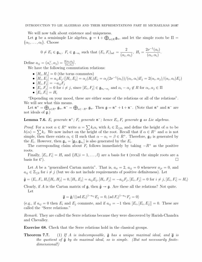
INTRODUCTION TO LIE ALGEBRAS AND THEIR REPRESENTATIONS PART III MICHAELMAS 201037
We will now talk about existence and uniqueness.Let g be a semisimple Lie algebra, g = t +
⊕α∈R gα, and let the simple roots be Π =
α1, . . . , αl. Choose
0 6= Ei ∈ gαi, Fi ∈ g−αi
such that (Ei, Fi)ad =2
(αi, αi), Hi =
2ν−1(αi)
(αi, αi).
Define aij = (α∨i , αj) =2(αi,αj)
(αi,αi).
We have the following commutation relations:
• [Hi, Hj] = 0 (the torus commutes)• [Hi, Ej] = aijEj ([Hi, Ej] = αj(Hi)Ej = αj(2ν
−1(αi))/(αi, αi)Ej = 2(αi, αj)/(αi, αi)Ej)• [Hi, Fj] = −aijFj
• [Ei, Fj] = 0 for i 6= j, since [Ei, Fj] ∈ gαi−αjand αi − αj 6∈ R for αi, αj ∈ Π
• [Ei, Fi] = Hi
“Depending on your mood, these are either some of the relations or all of the relations”.We will see what this means.
Let n+ =⊕
α∈R+ gα, n− =⊕
α∈−R+ gα. Then g = n+ + t + n−. (Note that n+ and n− arenot ideals of g.)
Lemma 7.6. Ei generate n+; Fi generate n−; hence Ei, Fi generate g as Lie algebras.
Proof. For a root α ∈ R+ write α =∑
kiαi with ki ∈ Z≥0, and define the height of α to beh(α) =
∑ki. We now induct on the height of the root. Recall that if α ∈ R+ and α is not
simple, then there exists αi ∈ Π such that α − αi = β ∈ R+. Therefore, gβ is generated bythe Ei. However, then gα = [gβ, gαi
] is also generated by the Ei.The corresponding claim about Fi follows immediately by taking −R+ as the positive
roots.Finally, [Ei, Fi] = Hi and Hi|i = 1, . . . , l are a basis for t (recall the simple roots are a
basis for t∗).
Let A be a “generalised Cartan matrix”. That is, aii = 2, aij = 0 whenever aji = 0, andaij ∈ Z≤0 for i 6= j (but we do not include requirements of positive definiteness). Let
g = 〈Ei, Fi, Hi|[Hi, Hj] = 0, [Hi, Ej] = aijEj, [Hi, Fj] = −aijFj, [Ei, Fj] = 0 for i 6= j, [Ei, Fi] = Hi〉
Clearly, if A is the Cartan matrix of g, then g g. Are these all the relations? Not quite.Let
g = g/〈(ad Ei)1−aijEj = 0, (ad Fi)
1−aijFj = 0〉(e.g., if aij = 0 then Ei and Ej commute, and if aij = −1 then [Ei, [Ei, Ej]] = 0. These arecalled the “Serre relations.”
Remark. They are called the Serre relations because they were discovered by Harish-Chandraand Chevalley.
Exercise 68. Check that the Serre relations hold in the classical groups.
Theorem 7.7. (1) If A is indecomposable, g has a unique maximal ideal, and g isthe quotient of g by its maximal ideal, so is simple. (But not necessarily finite-dimensional!)
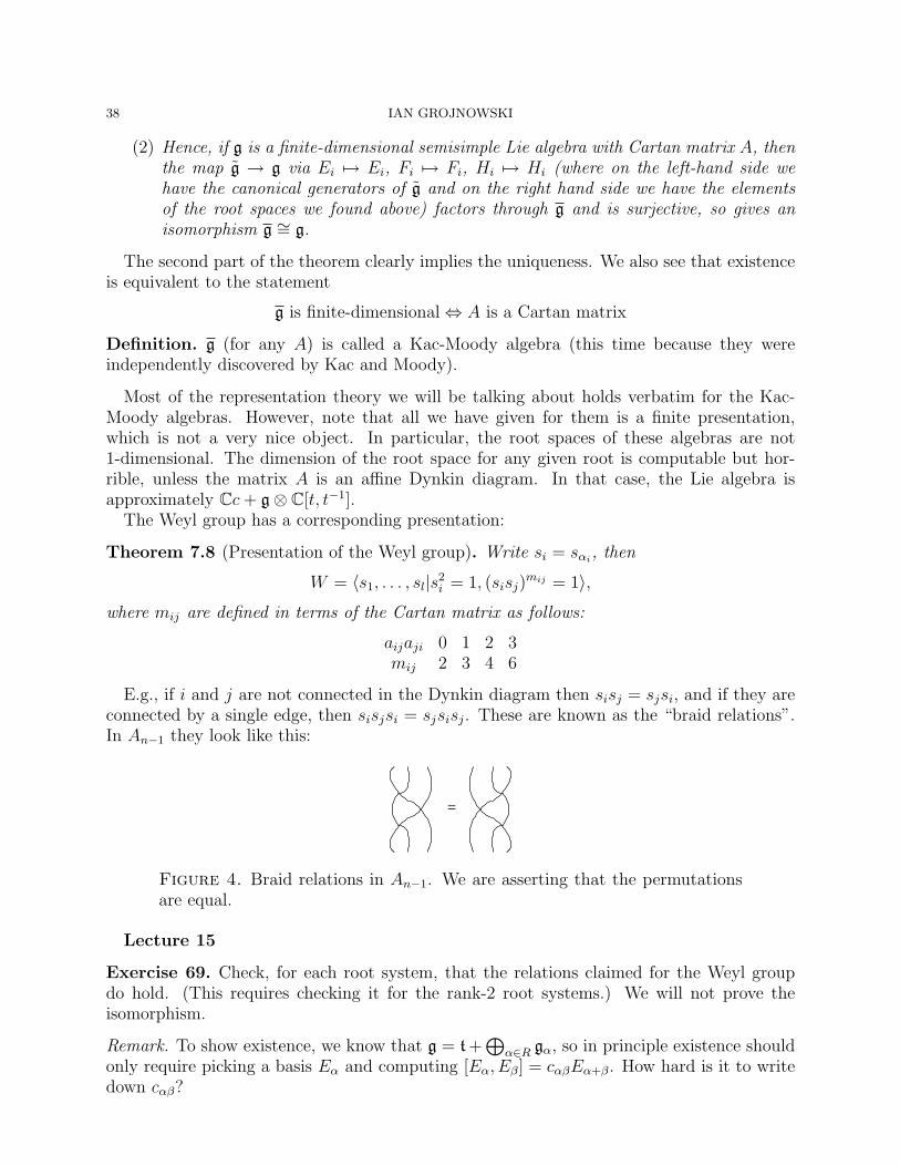
38 IAN GROJNOWSKI
(2) Hence, if g is a finite-dimensional semisimple Lie algebra with Cartan matrix A, thenthe map g → g via Ei 7→ Ei, Fi 7→ Fi, Hi 7→ Hi (where on the left-hand side wehave the canonical generators of g and on the right hand side we have the elementsof the root spaces we found above) factors through g and is surjective, so gives anisomorphism g ∼= g.
The second part of the theorem clearly implies the uniqueness. We also see that existenceis equivalent to the statement
g is finite-dimensional⇔ A is a Cartan matrix
Definition. g (for any A) is called a Kac-Moody algebra (this time because they wereindependently discovered by Kac and Moody).
Most of the representation theory we will be talking about holds verbatim for the Kac-Moody algebras. However, note that all we have given for them is a finite presentation,which is not a very nice object. In particular, the root spaces of these algebras are not1-dimensional. The dimension of the root space for any given root is computable but hor-rible, unless the matrix A is an affine Dynkin diagram. In that case, the Lie algebra isapproximately Cc + g⊗ C[t, t−1].
The Weyl group has a corresponding presentation:
Theorem 7.8 (Presentation of the Weyl group). Write si = sαi, then
W = 〈s1, . . . , sl|s2i = 1, (sisj)
mij = 1〉,where mij are defined in terms of the Cartan matrix as follows:
aijaji 0 1 2 3mij 2 3 4 6
E.g., if i and j are not connected in the Dynkin diagram then sisj = sjsi, and if they areconnected by a single edge, then sisjsi = sjsisj. These are known as the “braid relations”.In An−1 they look like this:
=
Figure 4. Braid relations in An−1. We are asserting that the permutationsare equal.
Lecture 15
Exercise 69. Check, for each root system, that the relations claimed for the Weyl groupdo hold. (This requires checking it for the rank-2 root systems.) We will not prove theisomorphism.
Remark. To show existence, we know that g = t +⊕
α∈R gα, so in principle existence shouldonly require picking a basis Eα and computing [Eα, Eβ] = cαβEα+β. How hard is it to writedown cαβ?

INTRODUCTION TO LIE ALGEBRAS AND THEIR REPRESENTATIONS PART III MICHAELMAS 201039
For a long time it was thought to be quite hard; however, with the discovery of the affineLie algebras, it turned out to be quite easy. We might even get to doing it for the ADEalgebras.
Remark. So far the status of existence of a finite-dimensional simple Lie algebra correspond-ing to an abstract root system for us is as fikkiws: we have shown that there exists asimple Lie algebra corresponding to each generalised Cartan matrix, but not that it is finite-dimensional. Suppose that for the g that we have defined we write g = t +
⊕α∈R gα (where
the torus comes from the root system). We can ask two questions: (1) what is the relation-ship between R and the root system we started with?; (2) What is the dimension of dim gα?While it is true that W · Π ⊆ R, in general there is not an equality between them. We callthe roots in W · Π “real roots” Rre; for the real roots, dim gα = 1. For finite-dimensionalLie algebras, all roots are real. If A is an affine Cartan matrix, then the semidefinite natureof it means that there exists a unique (up to scaling) root of length 0, called the imaginaryroot. The imaginary roots are pleasant and describable objects. For a general, indefinite,Cartan matrix, there exists an algorithm for computing dim gα, but the numbers are notvery meaningful.
8. Representations
Let g be a semisimple Lie algebra, g = t +⊕
α∈R gα = t + n+ + n−. Let V be a finite-dimensional representation of g. (We don’t quite need finite-dimensional; we’ll see exactlywhat we need a bit later.)
Proposition 8.1. (1) V =⊕
λ∈t∗ Vλ, where Vλ = v ∈ V |t(v) = λ(t)v ∀t ∈ t (this isthe weight space decomposition with respect to t)
(2) If Vλ 6= 0, then λ(hα) ∈ Z for all α ∈ R. (Here, hα is the element of the (sl2)α,hα = ν−1(α∨).)
Proof. Since V is a finite-dimensional representation of g, it is a finite-dimensional represen-tation of (sl2)α. Therefore, hα acts diagonalisably on V with λ(hα) ∈ Z. The first assertionfollows because hα span t.
Definition. Q = ZR =⊕
αi∈Π Zαi is the lattice of roots.P = γ ∈ QR|(γ, α∨) ∈ Z ∀α ∈ R (the dual lattice) is the lattice of weights. Note that thecondition can be checked by computing (γ, α∨i ) for αi ∈ Π.
Since, for β, α ∈ R we have (β, α∨) ∈ Z, we see Q ⊆ P . Also, if V is a finite-dimensionalrepresentation of g and Vλ 6= 0, then λ ∈ P , as λ(hα) = (λ, α∨).
Exercise 70. (1) |P/Q| <∞. In fact, |P/Q| = det A where A is the Cartan matrix.(2) W (P ) ⊆ P , where W is the Weyl group.
Example 8.1. In sl2, R = ±α, Q = Zα, (α, α) = 2, so P = Zα/2, and |P/Q| = 2 = det(2).
Definition. For V a finite-dimensional representation of g, define
ch V =∑λ∈P
dim Vλ · eλ ∈ Z[P ].
Here, eλ is a formal symbol (eλeµ = eλ+µ) forming a basis for Z[P ].
“People are looking at me as if I’m speaking some language I don’t speak, let alone youdon’t speak.”
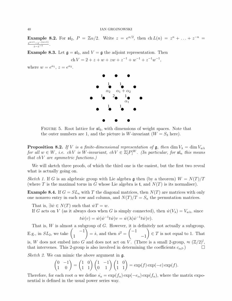
40 IAN GROJNOWSKI
Example 8.2. For sl2, P = Zα/2. Write z = eα/2, then ch L(n) = zn + . . . + z−n =zn+1−z−(n+1)
z−z−1 .
Example 8.3. Let g = sl3, and V = g the adjoint representation. Then
ch V = 2 + z + w + zw + z−1 + w−1 + z−1w−1,
where w = eα1 , z = eα2 .
1 1
2 11
1 1
α2 α1 + α2
α1
Figure 5. Root lattice for sl3, with dimensions of weight spaces. Note thatthe outer numbers are 1, and the picture is W -invariant (W = S3 here).
Proposition 8.2. If V is a finite-dimensional representation of g, then dim Vλ = dim Vwλ
for all w ∈ W , i.e. chV is W -invariant, chV ∈ Z[P ]W . (In particular, for sln this meansthat chV are symmetric functions.)
We will sketch three proofs, of which the third one is the easiest, but the first two revealwhat is actually going on.
Sketch 1. If G is an algebraic group with Lie algebra g then (by a theorem) W = N(T )/T(where T is the maximal torus in G whose Lie algebra is t, and N(T ) is its normaliser).
Example 8.4. If G = SLn with T the diagonal matrices, then N(T ) are matrices with onlyone nonzero entry in each row and column, and N(T )/T = Sn the permutation matrices.
That is, ∃w ∈ N(T ) such that wT = w.If G acts on V (as it always does when G is simply connected), then w(Vλ) = Vwλ, since
tw(v) = w(w−1tw)v = w(λ(w−1tw)v).
That is, W is almost a subgroup of G. However, it is definitely not actually a subgroup.
E.g., in SL2, we take
(−1
1
)= s, and then s2 =
(−1
−1
)∈ T is not equal to 1. That
is, W does not embed into G and does not act on V . (There is a small 2-group, ≈ (Z/2)l,that intervenes. This 2-group is also involved in determining the coefficients cαβ.)
Sketch 2. We can mimic the above argument in g.(0 −11 0
)=
(1 01 1
) (1 −10 1
) (1 01 1
)= exp(f) exp(−e) exp(f).
Therefore, for each root α we define sα = exp(fα) exp(−eα) exp(fα), where the matrix expo-nential is defined in the usual power series way.
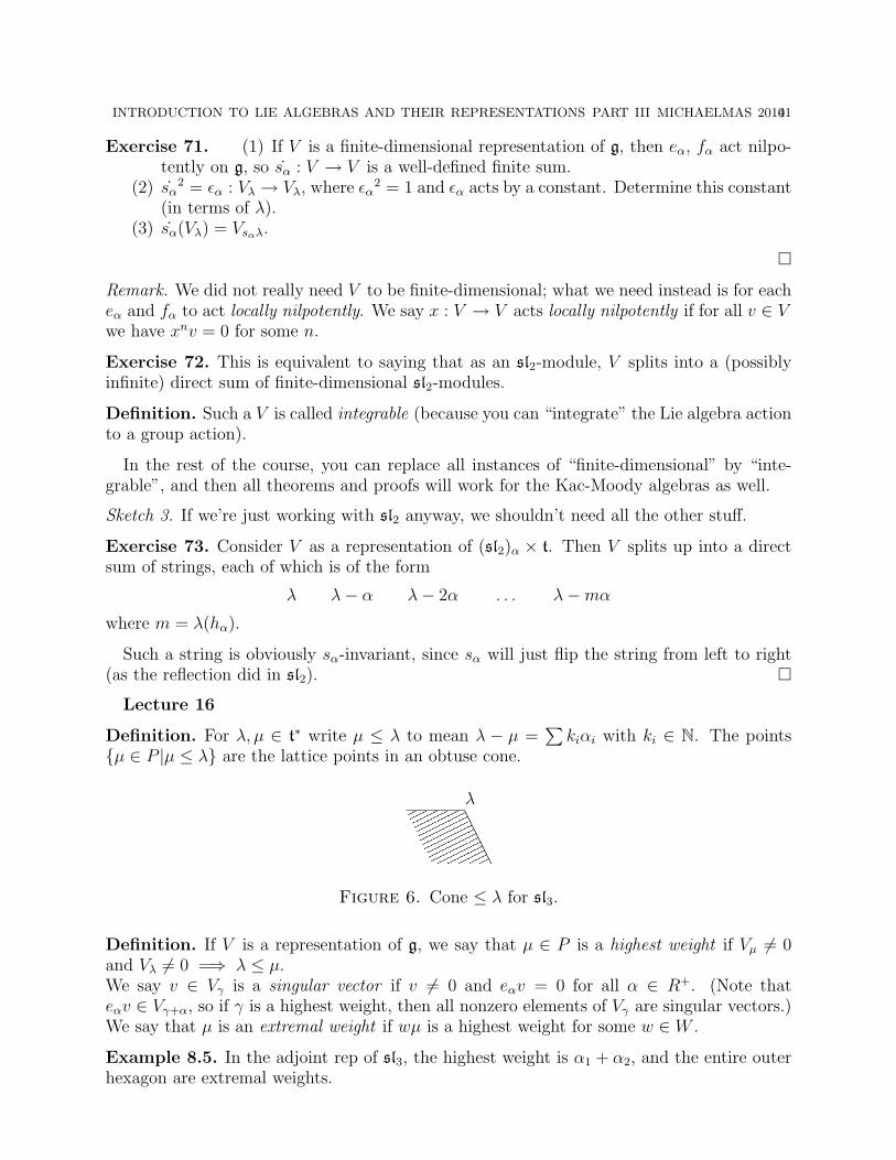
INTRODUCTION TO LIE ALGEBRAS AND THEIR REPRESENTATIONS PART III MICHAELMAS 201041
Exercise 71. (1) If V is a finite-dimensional representation of g, then eα, fα act nilpo-tently on g, so sα : V → V is a well-defined finite sum.
(2) sα2 = εα : Vλ → Vλ, where εα
2 = 1 and εα acts by a constant. Determine this constant(in terms of λ).
(3) sα(Vλ) = Vsαλ.
Remark. We did not really need V to be finite-dimensional; what we need instead is for eacheα and fα to act locally nilpotently. We say x : V → V acts locally nilpotently if for all v ∈ Vwe have xnv = 0 for some n.
Exercise 72. This is equivalent to saying that as an sl2-module, V splits into a (possiblyinfinite) direct sum of finite-dimensional sl2-modules.
Definition. Such a V is called integrable (because you can “integrate” the Lie algebra actionto a group action).
In the rest of the course, you can replace all instances of “finite-dimensional” by “inte-grable”, and then all theorems and proofs will work for the Kac-Moody algebras as well.
Sketch 3. If we’re just working with sl2 anyway, we shouldn’t need all the other stuff.
Exercise 73. Consider V as a representation of (sl2)α × t. Then V splits up into a directsum of strings, each of which is of the form
λ λ− α λ− 2α . . . λ−mα
where m = λ(hα).
Such a string is obviously sα-invariant, since sα will just flip the string from left to right(as the reflection did in sl2).
Lecture 16
Definition. For λ, µ ∈ t∗ write µ ≤ λ to mean λ − µ =∑
kiαi with ki ∈ N. The pointsµ ∈ P |µ ≤ λ are the lattice points in an obtuse cone.
λ
Figure 6. Cone ≤ λ for sl3.
Definition. If V is a representation of g, we say that µ ∈ P is a highest weight if Vµ 6= 0and Vλ 6= 0 =⇒ λ ≤ µ.We say v ∈ Vγ is a singular vector if v 6= 0 and eαv = 0 for all α ∈ R+. (Note thateαv ∈ Vγ+α, so if γ is a highest weight, then all nonzero elements of Vγ are singular vectors.)We say that µ is an extremal weight if wµ is a highest weight for some w ∈ W .
Example 8.5. In the adjoint rep of sl3, the highest weight is α1 + α2, and the entire outerhexagon are extremal weights.

42 IAN GROJNOWSKI
Theorem 8.3. g is a semisimple Lie algebra over C.
(1) “Complete reducibility”: if V is a finite-dimensional representation of g, then V is adirect sum of irreducible representations of g.
Set P+ = λ ∈ P : (λ, α∨) > 0 ∀α ∈ R+ (of course, it’s enough to check this onα ∈ Π). This is the cone of dominant weights. The assertion of the next parts of thetheorem is that P+ parametrises the finite-dimensional irreducible representations ofg, with λ 7→ L(λ). More precisely,
(2) Let V be a finite-dimensional irreducible representation of g, and v ∈ Vλ a singularvector. Then(a) dim Vλ = 1(b) Vµ 6= 0 =⇒ µ ≤ λ, so λ is a highest weight (and v a highest weight vector)(c) λ(hi) ∈ N for all i, i.e. λ ∈ P+.
Moreover, if W is another finite-dimensional irreducible representation of g withhighest weight λ, and w ∈ Wλ, w 6= 0, then there exists a unique isomorphismV → W mapping v 7→ w. (Of course, given they are irreducible representations,if there is an isomorphism, there is a one-dimensional family of them, so we wouldpin down the exact one by sending v 7→ w. That is, uniqueness is not the nontrivialstatement here.)
(3) Given λ ∈ P+, there exists a finite-dimensional irreducible representation with highestweight λ, called L(λ).
(4) A formula for chL(λ) (the Weyl character formula), to be stated later.
Remark. For Kac-Moody algebras, we need a slight modification, since it is no longer obviousthat we will have highest-weight vectors. We need to work in the category of integrablehighest-weight representations instead.
Corollary 8.4.
chL(λ) = eλ +∑µ<λ
aµλeµ ∈ Z[P ]
hence chL(λ)|λ ∈ P+ are linearly independent (they have different leading terms). On theother hand,
chL(λ) = mλ +∑µ<λ
aµλmµ ∈ Z[P ]W , where mµ =∑
γ∈Wµ
eγ.
Since mµ clearly form a basis for Z[P ]W , chL(λ) are a basis of Z[P ]W .
Corollary 8.5. If V and W are finite-dimensional representations of g, V ∼= W ⇔ chV =chW .
Proof. Complete reducibility + characters of irreducibles are a basis.
Definition. Define ωi ∈ P to be the dual basis to simple (co)roots, (ωi, α∨j ) = δij for
i = 1, . . . , l. These are called the fundamental weights.
Then P+ = ⊕Z≥0ωi = ∑
niωi|ni ≥ 0. This is a fundamental domain for the actionof W . Each irreducible representation will have a unique highest weight lying in this cone,which is what parametrises the representation.
Exercise 74. Compute ωi for the simple Lie algebras sln, so2n, so2n+1, sp2n, etc., and drawthe picture for A2, B2, and G2.

INTRODUCTION TO LIE ALGEBRAS AND THEIR REPRESENTATIONS PART III MICHAELMAS 201043
α2 α1 + α2
α1
Figure 7. Cone of positive weights for sl3. The adjoint representation’s high-est weight is α1 + α2.
Exercise 75. λ ∈ P =⇒ λ =∑
λ(hi)ωi, where hi = µ−1(α∨i ).
Example 8.6. For any g, the trivial representation is L(0).
For any simple g, the adjoint representation V = g is irreducible. The decompositiong = t +
⊕α∈R gα means that a highest weight λ is a root such that λ + αi 6∈ R for all i, i.e.
λ = θ, the highest root in R+. (Therefore, the theorem of the highest weight implies that θis unique, as promised.)
Example 8.7. In An−1, the highest root is θ = e1 − en (recall αi = ei − ei+1 and hi is adiagonal matrix with +1 in the ith position, −1 in the (i + 1)th position, and 0 elsewhere).We have θ(h1) = 1, θ(h2) = 0, . . . , θ(hn−2) = 0, θ(hn−1) = 1. We can label the Dynkindiagram by θ(hi):
. . .1 0 0 1
Figure 8. Adjoint representation of sln; labels are θ(hi), giving a decompo-sition of θ into fundamental weights.
Exercise 76. Compute θ(hi) for all the simple Lie algebras.
Example 8.8. Other representations of sln: we have the standard representation, Cn, withweight basis v1, . . . , vn and weights e1, . . . , en (recall
∑ei = 0). The highest weight is e1 (as
e1 > e2 > . . . > en, since e1 − e2, e2 − e3, . . . ∈ R+). Therefore, Cn = L(ω1), and
ch Cn = ee1 + . . . + een = z1 + . . . + zn
where zi = exp(ei) ∈ Z[P ] = Z[z±11 , . . . , z±1
n ]/(z1 . . . zn = 1).Now, if V and W are representations of g, then so is V ⊗W (via x ∈ g acts by x⊗1+1⊗x).
In particular, V ⊗ V is a representation. Note that σ : V ⊗ V → V ⊗ V , a ⊗ b 7→ b ⊗ a,commutes with the g-action, so eigenspaces of σ are g-modules. That is, S2V and Λ2V areg-modules. In general, these may not be irreducible, but they are for sln (provided V isirreducible, of course!), as we check below:
Consider ΛsCn (for s ≤ n− 1). This has weight basis vi1 ∧ . . . ∧ vis for i1 < . . . < is, andthe weight of this is ei1 + . . . + eis as is clear from the action. Therefore,
Ei(vi1 ∧ . . . ∧ vis) = 0 for all i ⇔ vi1 ∧ . . . ∧ vis = v1 ∧ . . . ∧ vs,

44 IAN GROJNOWSKI
i.e. this is the only singular vector. Note that its weight is ω = e1 + . . . + es and is the sthfundamental weight, as (ω, ei − ei+1) = δis. Therefore,
ΛsCn = L(ωs) is a fundamental representation.
In particular, Λn−1Cn ∼= (Cn)∗ = L(ωn−1).Consider SmCn. It has weight basis vi1 . . . vim with i1 ≤ . . . ≤ im and weight ei1 + . . .+eim .
We haveEi(vi1 . . . vim) = 0 for all i⇔ vi1 . . . vis = v1 . . . v1 = vm
1 ,
i.e. SmCn is an irreducible representation isomorphic to L(mω1).
Exercise 77. Check that the above is true. Compute ch ΛsCn, ch SmCn. Find a closedformula for the generating functions∑
m≥0
(ch SmCn)qm,∑m≥0
(ch ΛmCn)qm.
Lecture 17
Exercise 78. (1) If V and W are g-modules, V finite-dimensional, then V ∗ ⊗ W ∼=Hom (V, W ) as g-modules, via v∗ ⊗ w 7→ (v 7→ v∗(v) · w).
Remark. If V is a g-module, V ∗ is a g-module with action (x · λ)(v) = −λ(xv). The− sign comes from differentiating the group action, (x · g)(v) = g−1(xv).
(2) Show that if V = Cn and g = sln, then V ⊗ V ∗ ∼= sln ⊕ C, adjoint + trivialrepresentations (where the trivial representation comes from Id ∈ Hom g(V, V )). Incontrast, V ⊗ V ∼= S2V ⊕ Λ2V always.
Exercise 79. Let g = son or sp2l for 2l = n, and V = Cn.
(1) Compute the highest weight of this representation.(2) V ∼= V ∗ via the form defining g, so V ⊗ V has at least three components (since it
must have the trivial subrepresentation). Show that it has exactly three, describethem, and find the highest weights.
We will now devote ourselves to proving Theorem 8.3 classifying all the representations ofsimple Lie algebras.
Let g be any algebra with a non-degenerate invariant bilinear form (, ), e.g., g semisimpleand (, ) = (, )ad . Let x1, . . . , xN be a basis of g, and x1, . . . , xN the dual basis (so (xi, x
j) =δij).
Definition. Ω =∑
xixi is the Casimir of g.
Remark. For the moment, Ω is an operator on any representation of g. However, we will in amoment define the “universal enveloping algebra of g”, and that is where Ω naturally lives.
Lemma 8.6. For all x ∈ g, we have [Ω, x] = 0.
Proof 1, coordinate-based. [Ω, x] = [∑
xixi, x]. Since ad x is a derivation, we rewrite this as∑
xi[xi, x] +
∑[xi, x]xi.
Write [xi, x] =∑
aijxj and [xi, x] =
∑bijxj. Then
aij = ([xi, x], xj) = ([xj, xi], x)
bij = ([xi, x], xj) = ([xj, xi], x) = −aji
INTRODUCTION TO LIE ALGEBRAS AND THEIR REPRESENTATIONS PART III MICHAELMAS 201045
Thus,
[Ω, x] =∑
xixjaij +
∑xjx
ibij = 0.
Proof 2, without coordinates. We have maps of g-modules C → End (g) ∼= g ⊗ g∗ ∼= g ⊗ g(the first map is via λ 7→ λId , i.e. 1 7→
∑xi ⊗ xi; the last isomorphism is via the bilinear
form). Since g acts on V , we have a map of g-modules g → End (V ). Finally, we have amap of g-modules End (V )⊗ End (V )→ End (V ) by multiplication. This finally gives
C → g⊗ g∗ ∼= g⊗ g→ End (V )⊗ End (V )→ End (V )
sending 1 7→ Ω. Therefore, Ω generates a trivial g-submodule of End (V ), which is equivalentto saying [Ω, x] = 0 for all x ∈ g.
Now let g be semisimple, g = t ⊕⊕
α∈R gα, and (, )ad the Killing form. Choose abasis u1, . . . , ul of t, xα of gα; choose the dual basis u1, . . . , ul of t and x−α of g−α (sothat (xα, x−α) = 1). Normalise xα so that (xα, x−α)ad = 1, so that x−α = x−α. Then[xα, x−α] = ν−1(α) by definition. Now,
Ω =∑
uiui +
∑α∈R+
(xαx−α + x−αxα) =∑
uiui + 2
∑α∈R+
x−αxα +∑
α∈R+
ν−1(α).
Definition. ρ = 12
∑α∈R+ α.
Remark. Of course, there will be an exercise to compute ρ for all the simple Lie algebras.However, we will state this exercise later, when it’s more obvious what ρ is.
Remark. If you like algebraic geometry, this is the square root of the canonical bundle onthe flag variety.
Then
Ω =∑
uiui + 2ν−1(ρ) + 2
∑α∈R+
x−αxα
Lemma 8.7. Let V be a g-module, v ∈ V a singular vector with weight λ (i.e. n+v = 0 andtv = λ(t)v). Then Ωv = (|λ + ρ|2 − |ρ|2)v.
Proof. Apply the most recent version of Ω:
Ωv =(∑
λ(ui)λ(ui) + λ(2ν−1(ρ)))
v + 2∑
α∈R+
x−αxαv = ((λ, λ) + 2(λ, ρ))v.
In particular, if V is irreducible, Ω acts on V by (λ, λ) + 2(λ, ρ) by Schur’s lemma.
9. PBW theorem
Let g be any Lie algebra over a field k.
Definition. The universal enveloping algebra of g Ug is the associative algebra over k gen-erated by g with relations xy − yx = [x, y] for all x, y ∈ g.
46 IAN GROJNOWSKI
More formally, if V is a vector space over k, then
TV = k + V + V ⊗ V + V ⊗3 + . . . =⊕n≥0
V ⊗n
is the tensor algebra of V , and is the free associative algebra generated by V . Let J be thetwo-sided ideal in Tg generated by x⊗ y − y ⊗ x = [x, y] for all x, y ∈ g; then Ug = Tg/J .
Exercise 80. An enveloping algebra for g is a linear map i : g→ A, where A is an associativealgebra, and i(x)i(y) − i(y)i(x) = i([x, y]). (For example, if V is a representation of g, wecan take A = End (V ) and i the action map.) Show that Ug is initial in the category ofenveloping algebras, i.e. any such map i factors uniquely through Ug.
Remark. This is old terminology – anywhere other than the above exercise and old textbooks,“enveloping algebra” almost certainly means “universal enveloping algebra”.
The Casimir operator naturally lives in Ug; in fact, as we’ve shown, in the center Z(Ug).Observe that Tg is a graded algebra, but that the relations we are imposing on it are not
homogeneous (x ⊗ y and y ⊗ x have degree 2, while [x, y] has degree 1). Consequently, Ugis not graded. It is, however, filtered.
Define (Ug)n to be the span of products of ≤ n elements of g, then Un ⊆ Um for n ≤ m,and Un · Um ⊆ Un+m. (In particular, U0 ⊇ k, U1 ⊇ k + g, etc.)
Exercise 81. Show that if x ∈ Um and y ∈ Un, then [x, y] ∈ Un+m−1 (we clearly have[x, y] ∈ Un+m, and are asserting that in fact the degree is one lower). By abuse of notation,for x, y ∈ Ug we write [x, y] to mean xy − yx.
Definition. For a filtration F0 ⊆ F1 ⊆ . . . , we write gr (F ) = ⊕Fi/Fi−1. (We probably needFi to be a filtration of an algebra for this to make sense...) This is the associated gradedalgebra.
Theorem 9.1 (Poincare-Birkhoff-Witt).
grUg = ⊕(Ug)n/(Ug)n−1∼= Sg
Equivalently, if x1, . . . , xn is a basis for g, then xa11 xa2
2 . . . xann |ai ∈ Z≥0 is a basis for Ug.
In particular, g → Ug.
Exercise 82. (1) Show that the previous exercise, [Un,Um] ⊆ Un+m−1, implies that thereis a well-defined map S(g)→ grUg extending the map g 7→ g.
(2) Show that the map is surjective, or equivalently that ∏
xaii span Ug.
Therefore, the hard part of PBW theorem is injectivity. We will not prove the theorem.
Remark. The theorem should imply that Ug is a deformation of Sg (i.e. if we considerxy − yx = t[x, y] then for t = 0 we get Sg whereas for t = 1 – and, in fact, for generic tby renormalising – we get Ug). The shortest proof of the theorem is indeed via deformationtheory.
10. Back to representations
Exercise 83. If V is a representation of g and v ∈ V , then the g-submodule of V generatedby v is Ug · v.
Lecture 18
INTRODUCTION TO LIE ALGEBRAS AND THEIR REPRESENTATIONS PART III MICHAELMAS 201047
Definition. V is a highest weight module for g if ∃v ∈ V singular (i.e. n+v = 0 andt · v = λ(t)v for all t ∈ t and some λ ∈ t∗) such that V = Ug · v.
Note that in fact Un− · v = V .
Proof. PBW theorem (the easy direction) implies that if x1, . . . , xN is a basis of g thenxa1
1 . . . xaNN spans Ug. Taking a basis for g ordered “n−, then t, then n+”, we see Ug ∼=
Un− ⊗ Ut⊗ Un+, and Un+ · v = Ut · v = Cv ⊆ Un− · v (since n+ · v = 0).
Remark. If V is irreducible and finite-dimensional, it is a highest weight module (as it has asingular vector v, and Ug · v is a submodule).
Proposition 10.1. Let V be a highest weight module for g (not necessarily finite-dimensional),and let vΛ be a highest weight vector with highest weight Λ ∈ t∗.
(1) t acts diagonalisably on V , so V =⊕
λ∈D(Λ) Vλ, where
D(Λ) = Λ−∑
kiαi|ki ∈ Z≥0 = µ ∈ t∗|µ ≤ Λ
(the “descent” of Λ).(2) VΛ = CvΛ, and all other weight spaces are finite-dimensional.(3) V is irreducible if and only if all singular vectors are in VΛ.(4) Ω acts on V as |Λ + ρ|2 − |ρ|2
(5) If vλ is a singular vector, then |λ + ρ|2 = |Λ + ρ|2(6) If Λ ∈ RR, then there exist only finitely many λ such that Vλ contains a singular
vector.(7) V contains a unique maximal proper submodule I. I is graded by t, I = ⊕(I ∩ Vλ),
and I is the sum of all proper submodules of V .
Remark. The assumption in (6) is in fact unnecessary, but there isn’t quite a one-line proofin that case. Note that if V is finite-dimensional, then we in fact know that all weights liein QR, but we are not assuming finite dimensionality here.
Proof. As V = Un− · vΛ, expressions e−β1e−β2 . . . e−βrvΛ span V (where βi ∈ R+ and e−βi∈
g−βi). The weight of such an expression is Λ− β1 − β2 − . . .− βr.
Exercise 84. Prove it!
This implies (1) immediately, and (2) upon noticing that there are finitely many ways ofwriting λ = Λ− β1 − . . .− βr for βi ∈ R+.
(3): if vλ ∈ Vλ is a singular vector, then N = Ug · vλ = Un− · vλ is a submodule of V withweights in D(λ). Since λ 6= Λ, we have D(λ) ( D(Λ), whence N is a proper submodule.Thus, if there is a singular vector outside VΛ, then V is not irreducible.Conversely, if N ⊆ V is a proper submodule, then tN ⊆ N , so N is graded by t, and itsweights lie in D(Λ). Let λ = Λ−
∑kiαi be a weight in N , with αi ∈ Π and
∑ki minimal.
Since N is a proper submodule, λ 6= Λ so∑
ki > 0, and in that case any nonzero vector inNλ is singular (since λ + αi is not a weight of N for any simple αi).
(7): Any proper submodule of V is t-graded and does not contain vΛ. The sum of allproper submodules still does not contain vΛ, so it is the maximal proper submodule.
(4): for the singular vector vΛ we have ΩvΛ = (|Λ + ρ|2 − |ρ|2)vΛ. Since V = Ug · vΛ andΩ commutes with Ug, we see that Ω acts by the same constant on all of V .
(5) is now immediate (apply the same observation to any other singular vector).

48 IAN GROJNOWSKI
(6): if Vλ contains a signular vector, then |λ + ρ|2 = |Λ + ρ|2. This means that λ lies inthe intersection of a sphere in RR (compact) and D(Λ) (discrete), so there are only finitelymany such λ.
Definition. Let Λ ∈ t∗. A Verma module M(Λ) with highest weight Λ and highest weightvector vΛ is a universal module with highest weight Λ. That is, given any other highestweight module W with highest weight Λ and highest weight vector w, there exists a uniquemap M(Λ)→ W sending vΛ 7→ w.
Remark. Verma modules were also discovered by Harish-Chandra.
Proposition 10.2. Let Λ ∈ t∗. Then
(1) There exists a unique Verma module M(Λ).(2) There exists a unique irreducible highest-weight module of weight Λ, called L(Λ).
Proof. Uniqueness of M(Λ) is clear from universality. For existence, take
M(Λ) = Ug⊗Ub CΛ
where b = n+ + t and CΛ is the b-module on which n+ · v = 0 and t · v = Λ(t)v.
Remark. You should think of this as the induced representation.
More concretely,
M(Λ) = Ug/(left ideal generated by u− Λ(u) for all u ∈ Ub)
(where Λ is extended to act on b by 0 on n+).That is, M(Λ) is the module generated by g acting on 1 with relations n+1 = 0, t · 1 =
Λ(t)1 for all t ∈ t = JΛ, and only the relations these imply.If W is any other highest weight module of highest weight Λ, then W = Ug/J for some
J ⊇ JΛ, i.e. M(Λ) W .In particular, an irreducible highest-weight module must be of the form M(Λ)/I(Λ) where
I(Λ) is a maximal proper submodule of M(Λ). Since we showed that there exists a uniquemaximal proper submodule, L(Λ) is unique.
Proposition 10.3. Let R+ = β1, . . . , βr. Then ek1−β1
. . . ekr−βr
vΛ is a basis for M(Λ).
Proof. Immediate from the difficult direction of PBW theorem.
Corollary 10.4. Any irreducible finite-dimensional g-module is of the form L(Λ) for someΛ ∈ P+.
Proof. We know that the highest weight must lie in P+ by sl2 theory.
Example 10.1. g = sl2. The Verma module M(Λ) looks like this:
• − • − • − . . .vΛ FvΛ F 2vΛ
i.e. an infinite string.
Exercise 85. (1) Show that V (λ) = L(λ) unless λ ∈ Z≥0.(2) If λ ∈ Z≥0, show that V (λ) contains a unique proper submodule, spanned by F λ+1vλ,
F λ+2vλ, . . . (which is itself a Verma module). Recover the finite-dimensional irre-ducible representations.
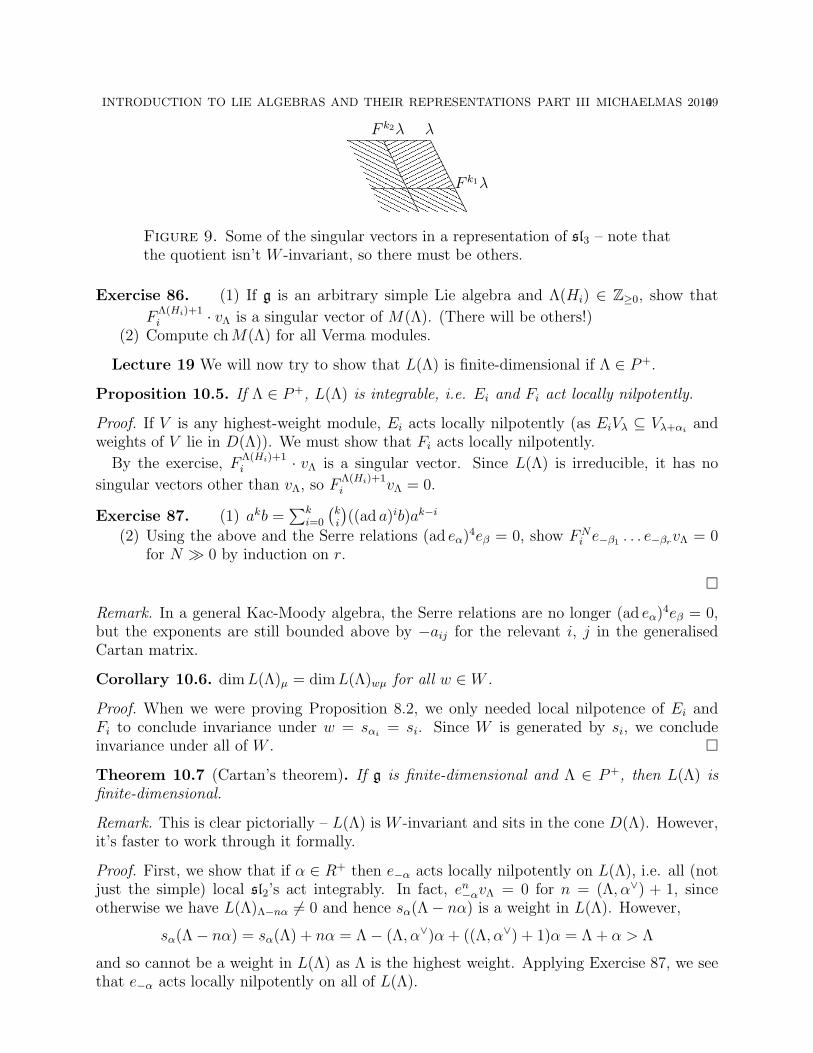
INTRODUCTION TO LIE ALGEBRAS AND THEIR REPRESENTATIONS PART III MICHAELMAS 201049
λF k2λ
F k1λ
Figure 9. Some of the singular vectors in a representation of sl3 – note thatthe quotient isn’t W -invariant, so there must be others.
Exercise 86. (1) If g is an arbitrary simple Lie algebra and Λ(Hi) ∈ Z≥0, show that
FΛ(Hi)+1i · vΛ is a singular vector of M(Λ). (There will be others!)
(2) Compute ch M(Λ) for all Verma modules.
Lecture 19 We will now try to show that L(Λ) is finite-dimensional if Λ ∈ P+.
Proposition 10.5. If Λ ∈ P+, L(Λ) is integrable, i.e. Ei and Fi act locally nilpotently.
Proof. If V is any highest-weight module, Ei acts locally nilpotently (as EiVλ ⊆ Vλ+αiand
weights of V lie in D(Λ)). We must show that Fi acts locally nilpotently.
By the exercise, FΛ(Hi)+1i · vΛ is a singular vector. Since L(Λ) is irreducible, it has no
singular vectors other than vΛ, so FΛ(Hi)+1i vΛ = 0.
Exercise 87. (1) akb =∑k
i=0
(ki
)((ad a)ib)ak−i
(2) Using the above and the Serre relations (ad eα)4eβ = 0, show FNi e−β1 . . . e−βrvΛ = 0
for N 0 by induction on r.
Remark. In a general Kac-Moody algebra, the Serre relations are no longer (ad eα)4eβ = 0,but the exponents are still bounded above by −aij for the relevant i, j in the generalisedCartan matrix.
Corollary 10.6. dim L(Λ)µ = dim L(Λ)wµ for all w ∈ W .
Proof. When we were proving Proposition 8.2, we only needed local nilpotence of Ei andFi to conclude invariance under w = sαi
= si. Since W is generated by si, we concludeinvariance under all of W .
Theorem 10.7 (Cartan’s theorem). If g is finite-dimensional and Λ ∈ P+, then L(Λ) isfinite-dimensional.
Remark. This is clear pictorially – L(Λ) is W -invariant and sits in the cone D(Λ). However,it’s faster to work through it formally.
Proof. First, we show that if α ∈ R+ then e−α acts locally nilpotently on L(Λ), i.e. all (notjust the simple) local sl2’s act integrably. In fact, en
−αvΛ = 0 for n = (Λ, α∨) + 1, sinceotherwise we have L(Λ)Λ−nα 6= 0 and hence sα(Λ− nα) is a weight in L(Λ). However,
sα(Λ− nα) = sα(Λ) + nα = Λ− (Λ, α∨)α + ((Λ, α∨) + 1)α = Λ + α > Λ
and so cannot be a weight in L(Λ) as Λ is the highest weight. Applying Exercise 87, we seethat e−α acts locally nilpotently on all of L(Λ).
50 IAN GROJNOWSKI
Therefore,
L(Λ) = U(n−)vΛ = ek1−β1
. . . ekr−βr
vΛ, R+ = β1, . . . , βr
is finite.
Lemma 10.8. si(R+ \ αi) = R+ \ αi.
Proof. Let α ∈ R+ \ αi, α =∑
j 6=i kjαj + kiαi with all kj ≥ 0 and some kj 6= 0. Note
that si(α) has the same coefficients on αj for j 6= i. Since R = R+ t −R+, we see si(α) 6∈−R+ =⇒ si(α) ∈ R+.
Lemma 10.9. Recall ρ = 12
∑α∈R+ α. Then ρ(Hi) = 1 for all i, i.e. ρ = ω1 + . . . + ωl.
Proof. Observe
siρ = si
1
2αi +
1
2
∑α 6=αi
α∈R+
α
= −1
2αi +
1
2
∑α 6=αi
α∈R+
α = ρ− αi.
On the other hand, siρ = ρ− (ρ, α∨i )αi, so (ρ, α∨i ) = 1 for all i.
Lemma 10.10 (Key lemma). Let Λ ∈ P+, µ + ρ ∈ P+, µ ≤ Λ. If |Λ + ρ| = |µ + ρ| thenΛ = µ.
Remark. This, again, is geometrically obvious from the fact that both D(Λ) and a sphereare convex.
Proof.
0 = (Λ + ρ, Λ + ρ)− (µ + ρ, µ + ρ) = (Λ− µ, Λ + (µ + ρ) + ρ)
Write Λ− µ =∑
kiαi, then since Λ + (µ + ρ) ∈ P+ and (ρ, αi) > 0 for all i, we see that wemust have ki = 0 for all i.
Theorem 10.11 (Weyl complete reducibility). Let g be a semisimple Lie algebra, char k = 0,k = k. Then every finite-dimensional g-module V is a direct sum of irreducibles.
Proof. Recall that V is completely reducible as an (sl2)α-module, V = ⊕Vλ.Consider V n+
= x ∈ V : n+x = 0. By Engel’s theorem, V n+ 6= 0.Since [t, n+] ⊆ n+, t acts on V n+
, so V n+=
⊕µ∈P V n+
µ .
Claim. For every vµ ∈ V n+
µ , the module L = Ug · vµ is irreducible.
Proof. L is a highest weight module with highest weight µ, so we must only show that ithas no other singular vectors. If λ is the weight of a singular vector in L, then λ ≤ µ, but|λ + ρ| = |µ + ρ| by considering the action of the Casimir. Since V , and therefore L, isfinite-dimensional, we must have Λ, µ ∈ P+. By the key lemma, λ = µ.
Consequently, V ′ = Ug · V n+is completely reducible: if v1, . . . , vr is a weight basis
for V n+with weights λ1, . . . , λr, then V ′ = L(λ1) ⊕ . . . ⊕ L(λr). It remains to show that
N = V/V ′ = 0.Suppose not. N is finite-dimensional, so Nn+ 6= 0. Let vλ ∈ Nn+
λ be a singular vector withλ ∈ P+. Lift vλ to vλ ∈ Vλ. Since vλ 6= 0 in N , we must have Eivλ 6= 0 ∈ Vλ+αi
for some i.

INTRODUCTION TO LIE ALGEBRAS AND THEIR REPRESENTATIONS PART III MICHAELMAS 201051
Note that Eivλ = 0, so Eivλ ∈ V ′. Consequently, the Casimir Ω acts on Eivλ by∣∣λ + ρ
∣∣2−|ρ|2 for some λ ∈ λ1, . . . , λr. On the other hand, since vλ was singular in N , Ω acts on vλ
by |λ + ρ|2 − |ρ|2. Since Ω commutes with Ei, we find∣∣λ + ρ
∣∣ = |λ + ρ|. Moreover, λ + αi
is a weight in L(λ), so λ + αi = λ−∑
kjαj, i.e. λ < λ. This, however, contradicts the keylemma.
Remark. The usual proof (in particular, Weyl’s own proof) of this theorem involves liftingthe integrable action to the group, and using the maximal compact subgroup (for which wehave complete reducibility because it has positive, finite measure). Somehow, the key lemmais the equivalent of a positive-definite metric.
Lemma 10.12. Let Λ ∈ t∗ and M(Λ) the Verma module. Then
chM(Λ) =eΛ∏
α∈R+(1− e−α).
Lecture 20
Proof. Let R+ = β1, . . . , βr. By PBW, the basis for M(Λ) is ek1−β1
. . . ekr−βr
vΛ for ki ∈ Z≥0,and the weight of such an element is Λ −
∑kiβi. Therefore, dim M(Λ)Λ−β is the number
of ways of writing β as∑
kiβi over βi ∈ R. This is precisely the coefficient of e−β in∏α∈R+(1− α)−1.
Write ∆ =∏
α∈R+(1− e−α). We have shown that ch M(Λ) = eΛ/∆.
Lemma 10.13. For all w ∈ W , w(eρ∆) = det w · eρ∆. Here, det : W → Z/2 gives thedeterminant of w acting on t∗ (±1).
Proof. Since W is generated by simple reflections, it suffices to check that si(eρ∆) = −eρ∆.
Indeed,
si(eρ∆) = si
eρ(1− e−αi)∏
α 6=αi
α∈R+
(1− e−α)
= eρ−αi(1 + e+αi)∏
α 6=αi
α∈R+
(1− e−α) = −eρ∆.
Lemma 10.14. (1) For any highest weight module V (Λ) with highest weight Λ thereexist coefficients aλ ≥ 0, λ ≤ Λ, such that
chV (Λ) =∑λ≤Λ
|λ+ρ|=|Λ+ρ|
aλchL(λ)
with aΛ = 1.(2) There exist coefficients bλ ∈ Z with bΛ = 1 such that
chL(Λ) =∑λ≤Λ
|λ+ρ|=|Λ+ρ|
bλchM(λ).
We write B(Λ) = λ ≤ Λ| |λ + ρ| = |Λ + ρ|. Recall that B(Λ) is a finite set.
Remark. We have shown that B(Λ) is finite when Λ ∈ RR, but it is true in general.

52 IAN GROJNOWSKI
Proof. First, note that (1) implies (2). Indeed, totally order B(Λ) so that λi ≤ λj =⇒ i ≤ j.Applying (1) to the Verma modules gives a system of equations relating ch M(λ) and ch L(λ)which is upper-triangular with 1’s on the diagonal. Inverting this system gives (2). (Note inparticular that the coefficients in (2) may be negative.)
We now prove (1). Recall that the weight spaces of a highest weight module are finite-dimensional. We induct on
∑µ∈B(Λ) dim V (Λ)µ.
If V (Λ) is irreducible, we clearly have (1). Otherwise, there exists µ ∈ B(Λ) with asingular vector vµ ∈ V (Λ)µ. Pick µ with the largest height of Λ − µ (recall the height of∑
kiαi is∑
ki). Then Ug · vµ ⊆ V (Λ) has no singular vectors, and is therefore irreducible,
L(µ). Setting V (Λ) = V (Λ)/L(µ), we see that V (Λ) is a highest-weight module with a
smaller value of∑
µ∈B(Λ) dim V (Λ)µ, and ch V (Λ) = ch V (Λ) + ch L(µ).
We will now compute ch L(Λ) for Λ ∈ P+.We know
ch L(Λ) =∑
λ∈B(Λ)
bλch M(λ) =∑
λ∈B(Λ)
bλeλ/∆.
Now, w(ch L(Λ)) = ch L(Λ) for all w ∈ W , and w(∆eρ) = det w ·∆eρ. Therefore,
eρ∆ch L(Λ) =∑
λ∈B(Λ)
bλeλ+ρ
is W -antiinvariant. We can therefore rewrite∑λ∈B(Λ)
bλeλ+ρ =
∑orbits of W on B(Λ) + ρ
bλ
∑w∈W
det w · ew(λ+ρ).
Now, if λ ∈ RR (which is true, since Λ ∈ P+), then W (λ+ρ) intersects x ∈ RR|(x, α∨i ) ≥ 0in exactly one point (this set is a fundamental domain for the W -action, and we won’t haveboundary problems because (ρ, α∨i ) = 1 > 0). Therefore, we can take a dominant weight asthe orbit representative. Note, however, that there is only one dominant weight in B(Λ),namely, Λ! (This was the Key Lemma 10.10.) Therefore, we derive
Theorem 10.15 (Weyl Character Formula).
chL(Λ) =
∑w∈W det w · ew(Λ+ρ)
eρ∏
α∈R+(1− e−α)=
∑w∈W
det w · chM(w(Λ + ρ)− ρ).
Example 10.2. Let g = sl2, and write z = eα/2. Then C[P ] = C[z, z−1] and ρ = z. Wehave
ch L(mα/2) = (zm+1 − z−(m+1))/(z − z−1)
as before.
Remark. The second expression for the character of L(Λ) looks like an Euler characteristic.In fact, it is: there is a complex of Verma modules whose cohomology are the irreduciblemodules. This is known as the “Bernstein-Gelfand-Gelfand” resolution.
The first expression comes from something like a cohomology of coherent line bundles,and is variously known as Euler-Grothendieck, Attiyah-Bott, and Attiyah-Singer.

INTRODUCTION TO LIE ALGEBRAS AND THEIR REPRESENTATIONS PART III MICHAELMAS 201053
Corollary 10.16. Since L(0) = C, we must have chL(0) = 1, so
eρ∏
α∈R+
(1− e−α) =∑w∈W
det w · ewρ.
This is known as the Weyl denominator identity.
Exercise 88. Let g = sln. Show that the Weyl denominator identity is equivalent to theVandermonde determinant
det
1 1 . . . 1z1 z2 . . . zn...
.... . .
...zn−11 zn−1
2 . . . zn−1n
=∏i<j
(zj − zi),
where we write zi = e−αi .
Corollary 10.17 (Weyl dimension formula).
dim L(Λ) =∏
α∈R+
(α, Λ + ρ)/(α, ρ).
Example 10.3. g = sl3 of type A2, R+ = α, β, α + β with ρ = α + β = ω1 + ω2. LetΛ = m1ω1 + m2ω2, then
α β α + β(·, Λ + ρ) m1 + 1 m2 + 1 m1 + m2 + 2
(·, ρ) 1 1 2
Therefore, the dimension of L(Λ) is 1/2(m1 + 1)(m2 + 1)(m1 + m2 + 2).
“Just to check that you too certainly know the dimensions of the irreducible representa-tions, let me state the obvious exercise.”
Exercise 89. Compute the dimensions of all the finite-dimensional irreducible representa-tions of B2 and G2.
Lecture 21
Remark. Let w ∈ W be written as w = si1si2 . . . sir where sik are simple reflections. Thendet w = (−1)r. The minimal r such that w can be written in this form is called the lengthfo w, denoted l(w). The Monoid Lemma asserts that you can get from one minimal-lengthexpression for w to another by repeatedly applying the braid relations.
Exercise 90. l(w) = #−R+ ∩ w−1R+ = l(w−1).
We now go back to our proof.
Proof. We know ch L(Λ) =∑
dim L(Λ)λeλ ∈ C[P ]. We would like to set eλ 7→ 1, but that
leads to a 0/0 expression in the Weyl character formula, which is hard to evaluate. Therefore,we will start by defining the homomorphism Fµ : C[P ]→ C(q), eλ 7→ q−(λ,µ). We would liketo evaluate F0(ch L(λ)), since F0(e
µ) = 1 for all µ.We apply Fµ to the Weyl denominator identity:
q−(ρ,µ)∏
α∈R+
(1− q(α,µ)) =∑w∈W
det wq−(wρ,µ) =∑w∈W
det wq−(ρ,w−1µ)
54 IAN GROJNOWSKI
since det w = det w−1 and (x, wy) = (w−1x, y) (i.e. the Weyl group is a subgroup of theorthogonal group of the inner product).
We now apply Fµ to the Weyl character formula:
Fµ(ch L(Λ)) =
∑w∈W det wq−(w(Λ+ρ),µ)
q−(ρ,µ)∏
α∈R+(1− q(α,µ))
provided (α, µ) 6= 0 for all α ∈ R+.Take µ = ρ (recall that (ρ, αi) > 0 for all simple roots αi, so (ρ, α) > 0 for all α ∈ R+).
Then
Fρ(ch L(Λ)) =∑
dim L(λ)λq−(λ,ρ) =
q−(ρ,Λ+ρ)∏
α∈R+(1− q(α,Λ+ρ))
q−(ρ,ρ)∏
α∈R+(1− q−(α,ρ))
where we used our expression for the Weyl denominator identity and applied it to the nu-merator.
Setting q = 1 and applying L’Hopital’s rule,
dim L(Λ) =∏
α∈R+
(Λ + ρ, α)
(ρ, α).
Remark. “You are now in a position to answer any question you choose to answer, if necessaryby brute force.” For example, let us decompose L(λ) ⊗ L(µ) =
∑mν
λµL(ν); we want tocompute the Littlewood-Richardson coefficients mν
λµ (recall that we had the Clebsch-Gordanrule for them in sl2).
Define : Z[P ] → Z[P ], eλ 7→ e−λ, and CT : Z[P ] → Z with eλ 7→ 0 unless λ = 0, ande0 7→ 1. Define (, ) : Z[P ]×Z[P ]→ Z by (f, g) = 1
|W |CT (fg∆∆), where ∆ =∏
α∈R+(1−e−α).
Claim. Let χλ = chL(λ), χµ = chL(µ), then (χλ, χµ) = δµν. (If our Lie algebra has typeA, then χλ are the Schur functions, and this is their orthogonality.)
Given this claim, we have mνλµ = (χλχµ, χν) is algorithmically computable. It was a
great surprise to everyone when it was discovered that actually there is a simpler and morebeautiful way of doing this.
Proof of claim.
(χλ, χµ) =1
|W |CT (
∑x,w∈W
ew(λ+ρ)−ρex(µ+ρ)−ρ det(wx))
However, CT (ew(λ+ρ)−x(µ+ρ)) = δwxδµλ, since for λ, µ ∈ R+ we have x−1w(λ+ρ) = µ+ρ =⇒x = w, λ = µ.
11. Principal sl2
Define ρL ∈ t∗ by (ρL, αi) = 1 for all αi ∈ Π. (Compare with ρ, which had (ρ, α∨i ) = 1.)
Exercise 91. Show ρL = 12
∑α∈R+ α∨. In particular, if R is simply laced, ρ = ρL.
Then (ρL, α) = ht(α) =∑
ki if we write α =∑
kiαi.
INTRODUCTION TO LIE ALGEBRAS AND THEIR REPRESENTATIONS PART III MICHAELMAS 201055
Exercise 92.
FρL(ch L(Λ)) = q−(Λ,ρL)∏
α∈R+
(1− q(Λ+ρ,α∨))
(1− qρ,α∨).
[Hint: apply FρL to the Weyl denominator identity for the Langlands dual Lie algebra withroot system R∨.]
Note that (λ + ρ, α∨)/(ρ, α∨) = (λ + ρ, α)/(ρ, α) as α∨ = 2α/(α, α), so we recoved thesame formula for Weyl dimension.
Definition. We call FρL(ch L(Λ)) the q-dimension of L(λ), denoted dimq L(Λ).
Proposition 11.1. dimq L(Λ) is a unimodal polynomial. More specifically, it lives in N[q2, q−2]Z/2
or qN[q2, q−2]Z/2 (depending on its degree), and the coefficients decrease as the absolute valueof the degree gets bigger.
Proof. We will show that dimq L(Λ) is the character of an sl2-module in which all “strings”have the same parity.
Set H = 2ν−1(ρL) ∈ t ⊆ g, and set E =∑
Ei.
Exercise 93. Check that [H, E] = 2E.
Writing H =∑
ciHi with ci ∈ C, set F =∑
ciFi.
Exercise 94. (1) Show that E, F, H generate a copy of sl2. This is called the principalsl2.
(2) Show that if Λ− γ is a weight of L(Λ), then (Λ− γ, 2ρL) ≡ (Λ, 2ρL) mod 2.(3) Derive the proposition.
Exercise 95. Write [n] = (qn − 1)/(q − 1), and [n]! = [n][n − 1] . . . [1]. Show that thefollowing polynomials are unimodal:[
n
k
]=
[n]!
[k]![n− k]!(1 + q)(1 + q2) . . . (1 + qn)
[Hint: for the first, apply the above arguments to g = sln and V = SkCn or ΛkCn+k.For the second, apply it to the spin representation of Bn = so2n+1; we will define the spinrepresentation next time.]
Remark. When is L(λ) ∼= L(λ)∗? Precisely when the lowest weight of L(λ) is −λ. The lowestweight of L(λ) is w0λ, where w0 is the (unique) maximal-length element of W which sendsall the positive roots to negative ones.
Now, for a representation V which is isomorphic to its dual V ∗, we get a bilinear form onV . This bilinear form is either symmetric or antisymmetric. By above, we see that we candetermine which it is by laboriously computing characters; but can we tell simply by lookingat λ?
The answer turns out to be yes. Indeed, the form will pair the highest-weight and thelowest-weight vector, and if we look at the principal sl2, it is a string from the highest-weightto the lowest-weight vector. Now, on the principal sl2 it is quite easy to see that the formis antisymmetric if the representation is L(n) with n odd, and symmetric if it is L(n) withn event. Thus, all we need to know is (the parity of) (λ, 2ρL). This is called the Schurindicator.
56 IAN GROJNOWSKI
Lecture 22
Exercise 96. Compute dimq L(θ), where L(θ) is the adjoint representation, for G2, A2,and B2. Then do it for all the classical groups. You will notice that L(θ)|principal sl2 =L(2e1) + . . . + L(2el) where l = rank g = dim t, e1, . . . , el ∈ N, and e1 = 1. The ei are calledthe exponents of the Weyl group, and the order of the Weyl group is |W | = (e1+1) . . . (el+1).
Compute |W | for E8.
12. Crystals
Let g be a semisimple Lie algebra, Π = α1, . . . , αl the simple roots, and P the weightlattice.
Definition. A crystal is a set B, 0 6∈ B, together with functions wt : B → P , ei : B →B t 0 fi : B → B t 0 such that
(1) If eib 6= 0, then wt(ei(b)) = wt(b) + αi; if fib 6= 0, then wt(fi(b)) = wt(b)− αi.
(2) For b, b′ ∈ B, eib = b′ if and only if b = fib′.
(3) Before we state the third defining property, we need to introduce slightly more nota-tion.
We can draw B as a graph. The vertices are b ∈ B, and the edges are b −→i
b′ if eib′ = b.
We say that this edge is “coloured by i”. This graph is known as the crystal graph.
Example 12.1. In sl2 the string
n→ n− 2→ n− 4→ . . .→ −n
is a crystal, where the weight of vertex i is iα/2.
Define εi(b) = maxn ≥ 0 : eni (b) 6= 0, and φi(b) = maxn ≥ 0 : fn
i (b) 6= 0.• → • → • →︸ ︷︷ ︸
εi
b→ . . .→ • → ·︸ ︷︷ ︸φi
In sl2, the sum εi(b) + φi(b) is the length of the string. On the other hand, if we are inthe highest-weight representation L(n) = L(nw) and wt(b) = n − 2k, then ε(b) = k andφ(b) = n − k, i.e. φ(b) − ε(b) = (wt(b), α∨). The third property of the Lie algebras is thatthis happens in general:
(3) φi(b)− εi(b) = (wt(b), α∨i ) for all αi ∈ Π.
Define Bµ = b ∈ B : wt(b) = µ.
Definition. For B1 and B2 crystals, we define the tensor product B1 ⊗ B2 as follows: as aset, B1 ⊗B2 = B1 ×B2, wt(b1 ⊗ b2) = wt(b1) + wt(b2), and
ei(b1⊗b2) =
(eib1)⊗ b2, if φi(b1) ≥ εi(b2)
b1 ⊗ (eib2), if φi(b1) < εi(b2)fi(b1⊗b2) =
(fib1)⊗ b2, if φi(b1) > εi(b2)
b1 ⊗ (fib2), if φi(b1) ≤ εi(b2)
That is, we are trying to recreate the picture in Figure 10 in each colour.
Exercise 97. Check that B1 ⊗B2 as defined above is a crystal.
Exercise 98. B1 ⊗ (B2 ⊗B3) ∼= (B1 ⊗B2)⊗B3 via b1 ⊗ (b2 ⊗ b3) 7→ (b1 ⊗ b2)⊗ b3.
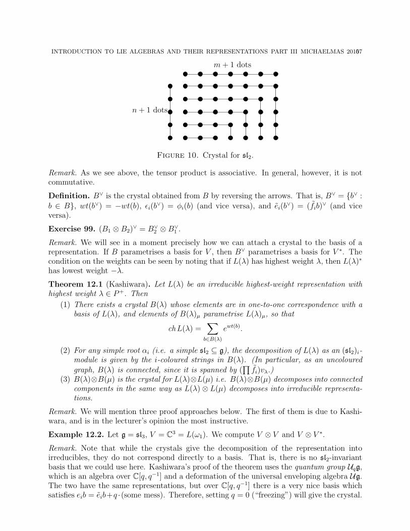
INTRODUCTION TO LIE ALGEBRAS AND THEIR REPRESENTATIONS PART III MICHAELMAS 201057
m + 1 dots
n + 1 dots
Figure 10. Crystal for sl2.
Remark. As we see above, the tensor product is associative. In general, however, it is notcommutative.
Definition. B∨ is the crystal obtained from B by reversing the arrows. That is, B∨ = b∨ :
b ∈ B, wt(b∨) = −wt(b), εi(b∨) = φi(b) (and vice versa), and ei(b
∨) = (fib)∨ (and vice
versa).
Exercise 99. (B1 ⊗B2)∨ = B∨2 ⊗B∨1 .
Remark. We will see in a moment precisely how we can attach a crystal to the basis of arepresentation. If B parametrises a basis for V , then B∨ parametrises a basis for V ∗. Thecondition on the weights can be seen by noting that if L(λ) has highest weight λ, then L(λ)∗
has lowest weight −λ.
Theorem 12.1 (Kashiwara). Let L(λ) be an irreducible highest-weight representation withhighest weight λ ∈ P+. Then
(1) There exists a crystal B(λ) whose elements are in one-to-one correspondence with abasis of L(λ), and elements of B(λ)µ parametrise L(λ)µ, so that
chL(λ) =∑
b∈B(λ)
ewt(b).
(2) For any simple root αi (i.e. a simple sl2 ⊆ g), the decomposition of L(λ) as an (sl2)i-module is given by the i-coloured strings in B(λ). (In particular, as an uncoloured
graph, B(λ) is connected, since it is spanned by (∏
fi)vλ.)(3) B(λ)⊗B(µ) is the crystal for L(λ)⊗L(µ) i.e. B(λ)⊗B(µ) decomposes into connected
components in the same way as L(λ)⊗ L(µ) decomposes into irreducible representa-tions.
Remark. We will mention three proof approaches below. The first of them is due to Kashi-wara, and is in the lecturer’s opinion the most instructive.
Example 12.2. Let g = sl3, V = C3 = L(ω1). We compute V ⊗ V and V ⊗ V ∗.
Remark. Note that while the crystals give the decomposition of the representation intoirreducibles, they do not correspond directly to a basis. That is, there is no sl2-invariantbasis that we could use here. Kashiwara’s proof of the theorem uses the quantum group Uqg,which is an algebra over C[q, q−1] and a deformation of the universal enveloping algebra Ug.The two have the same representations, but over C[q, q−1] there is a very nice basis whichsatisfies eib = eib+q ·(some mess). Therefore, setting q = 0 (“freezing”) will give the crystal.
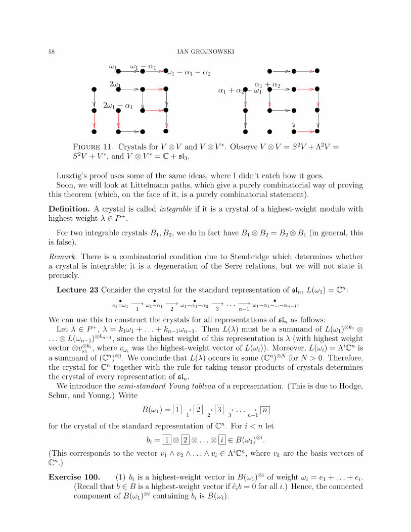
58 IAN GROJNOWSKI
ω1 − α1ω1
2ω1
2ω1 − α1
ω1 − α1 − α2
α1 + α2α1 + α2 − ω1
Figure 11. Crystals for V ⊗V and V ⊗V ∗. Observe V ⊗V = S2V +Λ2V =S2V + V ∗, and V ⊗ V ∗ = C + sl3.
Lusztig’s proof uses some of the same ideas, where I didn’t catch how it goes.Soon, we will look at Littelmann paths, which give a purely combinatorial way of proving
this theorem (which, on the face of it, is a purely combinatorial statement).
Definition. A crystal is called integrable if it is a crystal of a highest-weight module withhighest weight λ ∈ P+.
For two integrable crystals B1, B2, we do in fact have B1⊗B2 = B2⊗B1 (in general, thisis false).
Remark. There is a combinatorial condition due to Stembridge which determines whethera crystal is integrable; it is a degeneration of the Serre relations, but we will not state itprecisely.
Lecture 23 Consider the crystal for the standard representation of sln, L(ω1) = Cn:•
e1=ω1 −→1
•ω1−α1 −→
2
•ω1−α1−α2 −→
3. . . −→
n−1
•ω1−α1−...−αn−1.
We can use this to construct the crystals for all representations of sln as follows:Let λ ∈ P+, λ = k1ω1 + . . . + kn−1ωn−1. Then L(λ) must be a summand of L(ω1)
⊗k1 ⊗. . .⊗ L(ωn−1)
⊗kn−1 , since the highest weight of this representation is λ (with highest weightvector ⊗v⊗ki
ωi, where vωi
was the highest-weight vector of L(ωi)). Moreover, L(ωi) = ΛiCn isa summand of (Cn)⊗i. We conclude that L(λ) occurs in some (Cn)⊗N for N > 0. Therefore,the crystal for Cn together with the rule for taking tensor products of crystals determinesthe crystal of every representation of sln.
We introduce the semi-standard Young tableau of a representation. (This is due to Hodge,Schur, and Young.) Write
B(ω1) = 1 →1
2 →2
3 →3
. . . →n−1
n
for the crystal of the standard representation of Cn. For i < n let
bi = 1 ⊗ 2 ⊗ . . .⊗ i ∈ B(ω1)⊗i.
(This corresponds to the vector v1 ∧ v2 ∧ . . . ∧ vi ∈ ΛiCn, where vk are the basis vectors ofCn.)
Exercise 100. (1) bi is a highest-weight vector in B(ω1)⊗i of weight ωi = e1 + . . . + ei.
(Recall that b ∈ B is a highest-weight vector if eib = 0 for all i.) Hence, the connectedcomponent of B(ω1)
⊗i containing bi is B(ωi).
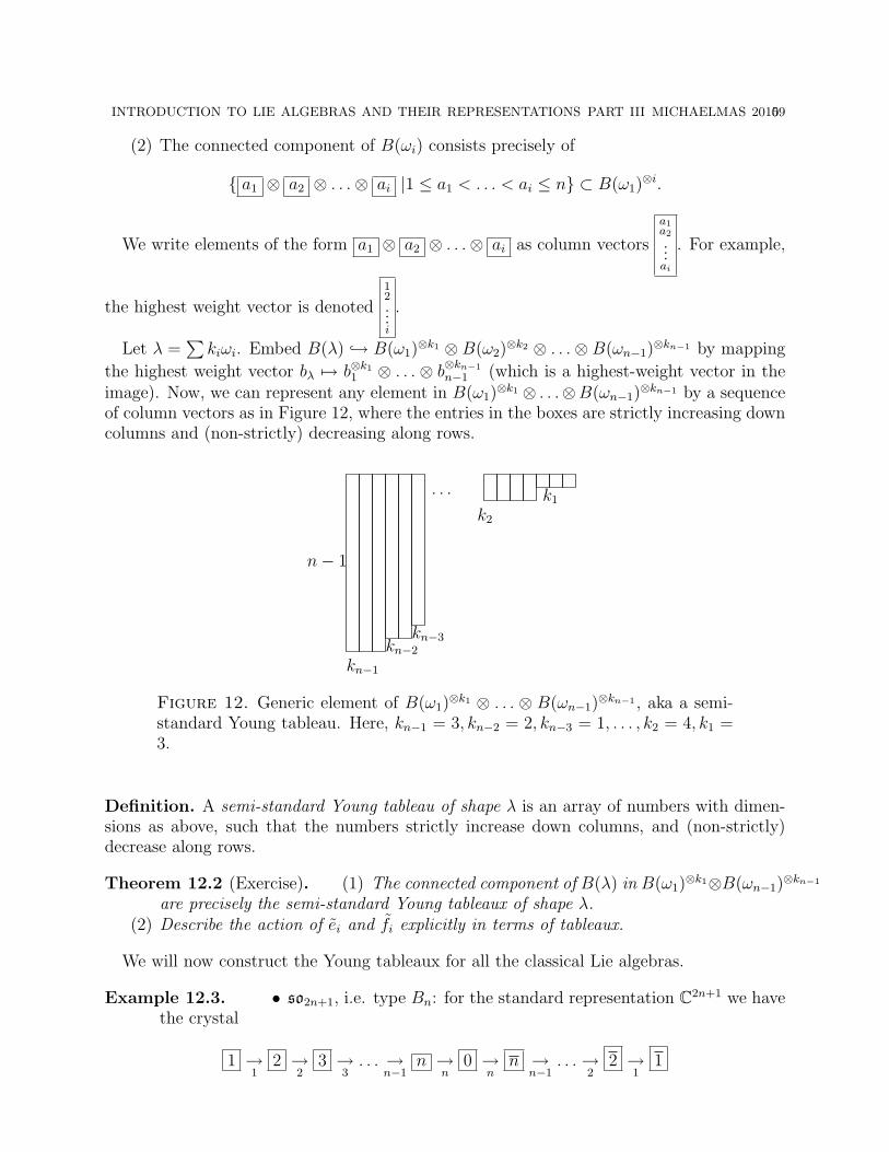
INTRODUCTION TO LIE ALGEBRAS AND THEIR REPRESENTATIONS PART III MICHAELMAS 201059
(2) The connected component of B(ωi) consists precisely of
a1 ⊗ a2 ⊗ . . .⊗ ai |1 ≤ a1 < . . . < ai ≤ n ⊂ B(ω1)⊗i.
We write elements of the form a1 ⊗ a2 ⊗ . . .⊗ ai as column vectors
a1a2
...ai
. For example,
the highest weight vector is denoted
12...i
.
Let λ =∑
kiωi. Embed B(λ) → B(ω1)⊗k1 ⊗ B(ω2)
⊗k2 ⊗ . . .⊗ B(ωn−1)⊗kn−1 by mapping
the highest weight vector bλ 7→ b⊗k11 ⊗ . . . ⊗ b
⊗kn−1
n−1 (which is a highest-weight vector in theimage). Now, we can represent any element in B(ω1)
⊗k1 ⊗ . . .⊗B(ωn−1)⊗kn−1 by a sequence
of column vectors as in Figure 12, where the entries in the boxes are strictly increasing downcolumns and (non-strictly) decreasing along rows.
. . .
n− 1
kn−1
kn−2
kn−3
k2
k1
Figure 12. Generic element of B(ω1)⊗k1 ⊗ . . . ⊗ B(ωn−1)
⊗kn−1 , aka a semi-standard Young tableau. Here, kn−1 = 3, kn−2 = 2, kn−3 = 1, . . . , k2 = 4, k1 =3.
Definition. A semi-standard Young tableau of shape λ is an array of numbers with dimen-sions as above, such that the numbers strictly increase down columns, and (non-strictly)decrease along rows.
Theorem 12.2 (Exercise). (1) The connected component of B(λ) in B(ω1)⊗k1⊗B(ωn−1)
⊗kn−1
are precisely the semi-standard Young tableaux of shape λ.(2) Describe the action of ei and fi explicitly in terms of tableaux.
We will now construct the Young tableaux for all the classical Lie algebras.
Example 12.3. • so2n+1, i.e. type Bn: for the standard representation C2n+1 we havethe crystal
1 →1
2 →2
3 →3
. . . →n−1
n →n
0 →n
n →n−1
. . .→2
2 →1
1
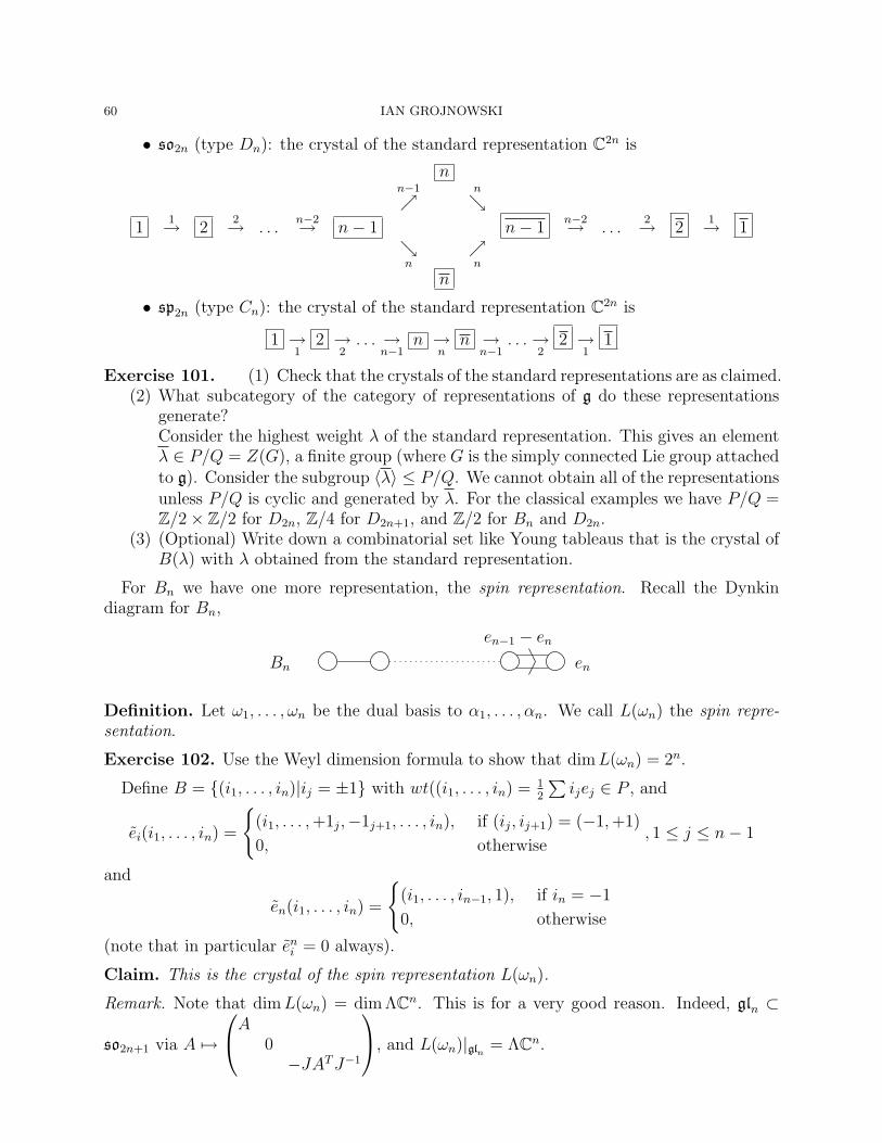
60 IAN GROJNOWSKI
• so2n (type Dn): the crystal of the standard representation C2n is
nn−1
n
1
1→ 22→ . . .
n−2→ n− 1 n− 1n−2→ . . .
2→ 21→ 1
n
n
n
• sp2n (type Cn): the crystal of the standard representation C2n is
1 →1
2 →2
. . . →n−1
n →n
n →n−1
. . .→2
2 →1
1
Exercise 101. (1) Check that the crystals of the standard representations are as claimed.(2) What subcategory of the category of representations of g do these representations
generate?Consider the highest weight λ of the standard representation. This gives an elementλ ∈ P/Q = Z(G), a finite group (where G is the simply connected Lie group attachedto g). Consider the subgroup 〈λ〉 ≤ P/Q. We cannot obtain all of the representationsunless P/Q is cyclic and generated by λ. For the classical examples we have P/Q =Z/2× Z/2 for D2n, Z/4 for D2n+1, and Z/2 for Bn and D2n.
(3) (Optional) Write down a combinatorial set like Young tableaus that is the crystal ofB(λ) with λ obtained from the standard representation.
For Bn we have one more representation, the spin representation. Recall the Dynkindiagram for Bn,
Bn
en−1 − en
en
Definition. Let ω1, . . . , ωn be the dual basis to α1, . . . , αn. We call L(ωn) the spin repre-sentation.
Exercise 102. Use the Weyl dimension formula to show that dim L(ωn) = 2n.
Define B = (i1, . . . , in)|ij = ±1 with wt((i1, . . . , in) = 12
∑ijej ∈ P , and
ei(i1, . . . , in) =
(i1, . . . , +1j,−1j+1, . . . , in), if (ij, ij+1) = (−1, +1)
0, otherwise, 1 ≤ j ≤ n− 1
and
en(i1, . . . , in) =
(i1, . . . , in−1, 1), if in = −1
0, otherwise
(note that in particular eni = 0 always).
Claim. This is the crystal of the spin representation L(ωn).
Remark. Note that dim L(ωn) = dim ΛCn. This is for a very good reason. Indeed, gln ⊂
so2n+1 via A 7→
A0−JAT J−1
, and L(ωn)|gln = ΛCn.
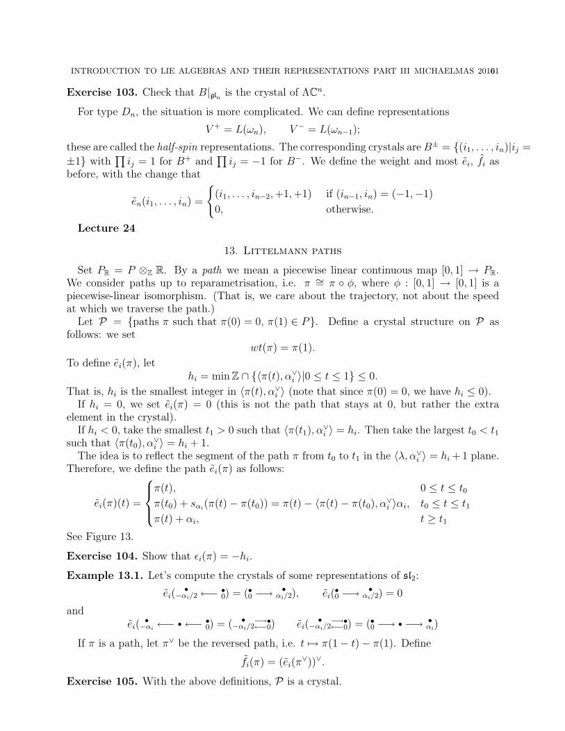
INTRODUCTION TO LIE ALGEBRAS AND THEIR REPRESENTATIONS PART III MICHAELMAS 201061
Exercise 103. Check that B|gln is the crystal of ΛCn.
For type Dn, the situation is more complicated. We can define representations
V + = L(ωn), V − = L(ωn−1);
these are called the half-spin representations. The corresponding crystals are B± = (i1, . . . , in)|ij =
±1 with∏
ij = 1 for B+ and∏
ij = −1 for B−. We define the weight and most ei, fi asbefore, with the change that
en(i1, . . . , in) =
(i1, . . . , in−2, +1, +1) if (in−1, in) = (−1,−1)
0, otherwise.
Lecture 24
13. Littelmann paths
Set PR = P ⊗Z R. By a path we mean a piecewise linear continuous map [0, 1] → PR.We consider paths up to reparametrisation, i.e. π ∼= π φ, where φ : [0, 1] → [0, 1] is apiecewise-linear isomorphism. (That is, we care about the trajectory, not about the speedat which we traverse the path.)
Let P = paths π such that π(0) = 0, π(1) ∈ P. Define a crystal structure on P asfollows: we set
wt(π) = π(1).
To define ei(π), lethi = min Z ∩ 〈π(t), α∨i 〉|0 ≤ t ≤ 1 ≤ 0.
That is, hi is the smallest integer in 〈π(t), α∨i 〉 (note that since π(0) = 0, we have hi ≤ 0).If hi = 0, we set ei(π) = 0 (this is not the path that stays at 0, but rather the extra
element in the crystal).If hi < 0, take the smallest t1 > 0 such that 〈π(t1), α
∨i 〉 = hi. Then take the largest t0 < t1
such that 〈π(t0), α∨i 〉 = hi + 1.
The idea is to reflect the segment of the path π from t0 to t1 in the 〈λ, α∨i 〉 = hi +1 plane.Therefore, we define the path ei(π) as follows:
ei(π)(t) =
π(t), 0 ≤ t ≤ t0π(t0) + sαi
(π(t)− π(t0)) = π(t)− 〈π(t)− π(t0), α∨i 〉αi, t0 ≤ t ≤ t1
π(t) + αi, t ≥ t1
See Figure 13.
Exercise 104. Show that εi(π) = −hi.
Example 13.1. Let’s compute the crystals of some representations of sl2:
ei(•
−αi/2←− •0) = (•0 −→ •αi/2), ei(
•0 −→ •
αi/2) = 0
andei(
•−αi ←− •←− •0) = ( •
−αi/2−→←−•0) ei(
•−αi/2
−→←−•0) = (•0 −→ • −→ •
αi)
If π is a path, let π∨ be the reversed path, i.e. t 7→ π(1− t)− π(1). Define
fi(π) = (ei(π∨))∨.
Exercise 105. With the above definitions, P is a crystal.
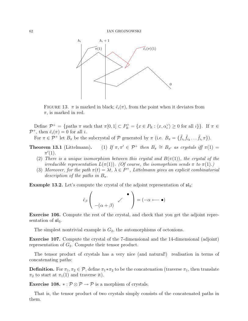
62 IAN GROJNOWSKI
0
hi hi + 1
π(1) ei(π)(1)
Figure 13. π is marked in black; ei(π), from the point when it deviates fromπ, is marked in red.
Define P+ = paths π such that π[0, 1] ⊂ P+R = x ∈ PR : 〈x, α∨i 〉 ≥ 0 for all i. If π ∈
P+, then ei(π) = 0 for all i.
For π ∈ P+ let Bπ be the subcrystal of P generated by π (i.e. Bπ = fi1 fi2 . . . firπ).
Theorem 13.1 (Littelmann). (1) If π, π′ ∈ P+ then Bπ∼= Bπ′ as crystals iff π(1) =
π′(1).(2) There is a unique isomorphism between this crystal and B(π(1)), the crystal of the
irreducible representation L(π(1)). (Of course, the isomoprhism sends π to π(1).)(3) Moreover, for the path π(t) = λt, λ ∈ P+, Littelmann gives an explicit combinatorial
description of the paths in Bπ.
Example 13.2. Let’s compute the crystal of the adjoint representation of sl3:
eβ
•
−(α + β)
= (−α←− •)
Exercise 106. Compute the rest of the crystal, and check that you get the adjoint repre-sentation of sl3.
The simplest nontrivial example is G2, the automorphisms of octonions.
Exercise 107. Compute the crystal of the 7-dimensional and the 14-dimensional (adjoint)representation of G2. Compute their tensor product.
The tensor product of crystals has a very nice (and natural!) realisation in terms ofconcatenating paths:
Definition. For π1, π2 ∈ P , define π1∗π2 to be the concatenation (traverse π1, then translateπ2 to start at π1(1) and traverse it).
Exercise 108. ∗ : P ⊗ P → P is a morphism of crystals.
That is, the tensor product of two crystals simply consists of the concatenated paths inthem.

INTRODUCTION TO LIE ALGEBRAS AND THEIR REPRESENTATIONS PART III MICHAELMAS 201063
Remark. We have now defined B(λ) explicitly without using L(λ). One can prove the Weylcharacter formula
ch B(λ) =
∑w∈W det wew(λ+ρ)− ρ∏
α∈R+(1− e−α)
from this, without referring to L(λ) or quantum groups. To do this, one builds ch L(λ) andL(λ) itself one root at a time, and uses the Demazure character formula.
More specifically: ∀w ∈ W consider Lw(λ), the n+-submodule of L(λ) generated by vwλ,where vλ is the highest weight vector. (Equivalently, it is the submodule generated by the1-dimensional space wL(λ)λ.)
Theorem 13.2 (Demazure character formula).
chLw(λ) = Dw(eλ),
where we write w = si1 . . . sir a reduced (i.e. shortest) decomposition, and set
Dw = Dsi1. . . Dsir
, Dsi(f) =
f − e−αisi(f)
1− e−αi= (1+si)
f
1− e−αi=
1
eαi/2 − e−αi/2(feαi/2−si(feαi/2)).
That is,
Dsi(eλ) =
eλ + eλ−αi + . . . + esiλ, 〈λ, α∨i 〉 ≥ 0
0, 〈λ, α∨i 〉 = −1
−(eλ+αi + . . . + esiλ−αi), 〈λ, α∨i 〉 < −1.
“I’ve got about six minutes. Is that enough time to tell you about the Langlands program?”Suppose that G is an algebraic group with Lie algebra g which is semisimple. For a given
g, there is the smallest group G above it, Gad = G/ZG (whose centre is 1). There is alsothe largest group, Gsc the simply connected cover of G, which is still an algebraic group. Wehave π1(G
ad ) = (P/Q)∗ and ZGsc = P/Q.(For example, SLn is the simply connected group, and PSLn is the adjoint group.)In this course we have studied the category Rep g = Rep Gsc.Recall that for G a finite group, the number of irreducible representations is the number
of conjugacy classes, but conjugacy classes do not parametrise the representations. For us,however, the representations are parametrised by P+ = P/W .
It is possible, for G an algebraic group, to define LG, the Langlands dual group, wherethe Lie algebra g and the root system R correspond to g∨ and R∨ (and in fact the torus andthe dual torus will swap in the dual group).
If we consider the representations of G(F ) where F = Fq or F = C((t)), these correspondroughly to conjugacy classes of homomorphisms (W (F ) → LG(C))/LG(C), where W (F ) isa “thickening” of the Galois group of F .


![Lie Algebras - University of Idahobrooksr/liealgebraclass.pdf · volumes [1], Lie Groups and Lie Algebras, Chapters 1-3, [2], Lie Groups and Lie Algebras, Chapters 4-6, and [3], Lie](https://img.dokumen.tips/doc/110x75/5ec51f9cde3711693f3d65c7/lie-algebras-university-of-idaho-brooksrliealgebraclasspdf-volumes-1-lie.jpg)