Introduction to latent variable models - econ.upf.edumichael/latentvariables/lecture1.pdfItem Response Theory models: models for items (categorical responses) measuring a common latent

Introduction to latent variable models

lecture 1

Francesco BartolucciDepartment of Economics, Finance and Statistics

University of Perugia, IT

[email protected]

– Typeset by FoilTEX – 1

[2/24]

Outline

• Latent variables and their use

• Some example datasets

• A general formulation of latent variable models

• The Expectation-Maximization algorithm for maximum likelihood

estimation

• Finite mixture model (with example of application)

• Latent class and latent regression models (with examples of

application)


Latent variables and their use [3/24]

Latent variable and their use

• A latent variable is a variable which is not directly observable and is

assumed to affect the response variables (manifest variables)

• Latent variables are typically included in an econometric/statistical

model (latent variable model) with different aims:

. representing the effect of unobservable covariates/factors and then

accounting for the unobserved heterogeneity between subjects

(latent variables are used to represent the effect of these

unobservable factors)

. accounting for measurement errors (the latent variables represent

the “true” outcomes and the manifest variables represent their

“disturbed” versions)



. summarizing different measurements of the same (directly)

unobservable characteristics (e.g., quality-of-life), so that sample

units may be easily ordered/classified on the basis of these traits

(represented by the latent variables)

• Latent variable models have now a wide range of applications,

especially in the presence of repeated observations, longitudinal/panel

data, and multilevel data

• These models are typically classified according to:

. nature of the response variables (discrete or continuous)

. nature of the latent variables (discrete or continuous)

. inclusion or not of individual covariates



Most well-known latent variable models

• Factor analysis model: fundamental tool in multivariate statistic to

summarize several (continuous) measurements through a small

number of (continuous) latent traits; no covariates are included

• Item Response Theory models: models for items (categorical

responses) measuring a common latent trait assumed to be

continuous (or less often discrete) and typically representing an

ability or a psychological attitude; the most important IRT model

was proposed by Rasch (1961); typically no covariates are included

• Generalized linear mixed models (random-effects models): extension

of the class of Generalized linear models (GLM) for continuous or

categorical responses which account for unobserved heterogeneity,

beyond the effect of observable covariates



• Finite mixture model: model, used even for a single response variable,

in which subjects are assumed to come from subpopulations having

different distributions of the response variables; typically covariates

are ruled out

• Latent class model: model for categorical response variables based on

a discrete latent variable, the levels of which correspond to latent

classes in the population; typically covariates are ruled out

• Finite mixture regression model (Latent regression model): version of

the finite mixture (or latent class model) which includes observable

covariates affecting the conditional distribution of the response

variables and/or the distribution of the latent variables



• Models for longitudinal/panel data based on a state-space

formulation: models in which the response variables (categorical or

continuous) are assumed to depend on a latent process made of

continuous latent variables

• Latent Markov models: models for longitudinal data in which the

response variables are assumed to depend on an unobservable Markov

chain, as in hidden Markov models for time series; covariates may be

included in different ways

• Latent Growth/Curve models: models based on a random effects

formulation which are used the study of the evolution of a

phenomenon across of time on the basis of longitudinal data;

covariates are typically ruled out



Some example datasets

• Dataset 1: it consists of 500 observations simulated from a model

with 2 components

• By a finite mixture model we can estimate separate parameters for

these components and classify sample units (model-based clustering)



• Dataset 2: it is collected on 216 subjects who responded to T = 4

items concerning similar social aspects (Goodman, 1974, Biometrika)

• Data may be represented by a 24-dimensional vector of frequencies

for all the response configurations

n =

freq(0000)

freq(0001)...

freq(1111)

=

42

23...

20

• By a latent class model we can classify subjects in homogeneous

clusters on the basis of the tendency measured by the items



• Dataset 3: about 1,093 elderly people, admitted in 2003 to 11

nursing homes in Umbria (IT), who responded to 9 items about their

health status:

Item %

1 [CC1] Does the patient show problems in recalling what

recently happened (5 minutes)? 72.6

2 [CC2] Does the patient show problems in making decisions

regarding tasks of daily life? 64.2

3 [CC3] Does the patient have problems in being understood? 43.9

4 [ADL1] Does the patient need support in moving to/from lying position,

turning side to side and positioning body while in bed? 54.4

5 [ADL2] Does the patient need support in moving to/from bed, chair,

wheelchair and standing position? 59.0

6 [ADL3] Does the patient need support for eating? 28.7

7 [ADL4] Does the patient need support for using the toilet room? 63.5

8 [SC1] Does the patient show presence of pressure ulcers? 15.4

9 [SC2] Does the patient show presence of other ulcers? 23.1



• Binary responses to items are coded so that 1 is a sign of bad health

conditions

• The available covariates are:

. gender (0 = male, 1 = female)

. 11 dummies for the nursing homes

. age

• By a latent class regression model we can understand how the

covariates affect the probability of belonging to the different latent

classes (corresponding to different levels of the health status)


General formulation of latent variable models [12/24]

A general formulation of latent variable models

• The contexts of application dealt with are those of:

. observation of different response variables at the same occasion

(e.g. item responses)

. repeated observations of the same response variable at consecutive

occasions (longitudinal/panel data); this is related to the multilevel

case in which subjects are collected in clusters

• Basic notation:

. n: number of sample units (or clusters in the multilevel case)

. T : number of response variables (or observations of the same

response variable) for each subject

. yit: response variable of type t (or at occasion t) for subject i

. xit: corresponding column vector of covariates



• A latent variable model formulates the conditional distribution of the

response vector yi = (yi1, . . . , yiT )′, given the covariates (if there

are) in Xi = (xi1, . . . ,xiT ) and a vector ui = (ui1, . . . , uil)′ of

latent variables

• The model components of main interest concern:

. conditional distribution of the response variables given Xi and ui

(measurement model): p(yi|ui,Xi)

. distribution of the latent variables given the covariates (latent

model): p(ui|Xi)

• With T > 1, a crucial assumption is typically that of (local

independence): the response variables in yi are conditionally

independent given Xi and ui



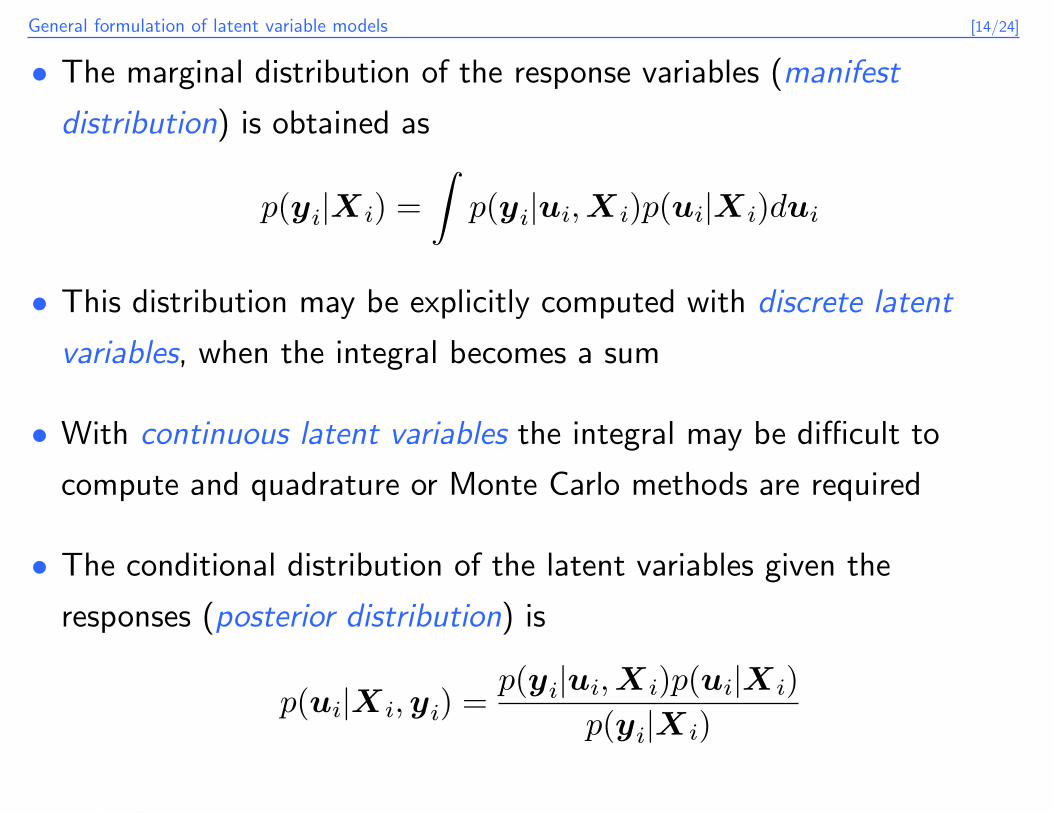
• The marginal distribution of the response variables (manifest

distribution) is obtained as

p(yi|Xi) =

∫p(yi|ui,Xi)p(ui|Xi)dui

• This distribution may be explicitly computed with discrete latent

variables, when the integral becomes a sum

• With continuous latent variables the integral may be difficult to

compute and quadrature or Monte Carlo methods are required

• The conditional distribution of the latent variables given the

responses (posterior distribution) is

p(ui|Xi,yi) =p(yi|ui,Xi)p(ui|Xi)

p(yi|Xi)



Case of discrete latent variables(finite mixture model, latent class model)

• Each vector ui has a discrete distribution with k support point

ξ1, . . . , ξk and corresponding probabilities π1(Xi), . . . , πk(Xi)

(possibly depending on the covariates)

• The manifest distribution is then

p(yi|Xi) =∑c

πcp(yi|ui = ξc,Xi) without covariates

p(yi|Xi) =∑c

πc(Xi)p(yi|ui = ξc,Xi) with covariates

• Model parameters are typically the support points ξc, the mass

probabilities πc and parameters common to all the distributions



Example: Finite mixture of Normal distributionswith common variance

• There is only one latent variable (l = 1) having k support points and

no covariates are included

• Each support point ξc corresponds to a mean µc and there is a

common variance-covariance matrix Σ

• The manifest distribution of yi is: p(yi) =∑

c πcφ(yi;µc,Σ)

. φ(y;µ,Σ): density function of the multivariate Normal distribution

with mean µ and variance-covariance matrix Σ

• Exercise: write down the density of the model in the univariate case

with k = 2 and represent it for different parameter values



Case of continuous latent variables(Generalized linear mixed models)

• With only one latent variable (l = 1), the integral involved in the

manifest distribution is approximated by a sum (quadrature method):

p(yi|Xi) ≈∑c

πcp(yi|ui = ξc,Xi)

• In this case the nodes ξc and the corresponding weights πc are a priori

fixed; a few nodes are usually enough for an adequate approximation

• With more latent variables (l > 1), the quadrature method may be

difficult to implement and unprecise; a Monte Carlo method is

preferable in which the integral is approximated by a mean over a

sample drawn from the distribution of ui



Example: Logistic model with random effect

• There is only one latent variable ui (l = 1), having Normal

distribution with mean µ and variance σ2

• The distribution of the response variables given the covariates is

p(yit|ui,Xi) = p(yit|ui,xit) =exp[yit(ui + x

′itβ)]

1 + exp(ui + x′itβ)

and local independence is assumed

• The manifest distribution of the response variables is

p(yi|Xi) =

∫[∏t

p(yit|ui,xit)]φ(ui;µ, σ2)dui



• In order to compute the manifest distribution it is convenient to

reformulate the model as

p(yit|ui,xit) =exp(uiσ + x′itβ)

1 + exp(uiσ + x′itβ),

where ui ∼ N(0, 1) and µ has been absorbed into the intercept in β

• The manifest distribution is computed as

p(yi|Xi) =∑c

πc∏t

p(yit|ui = ξc,xit)

. ξ1, . . . , ξk: grid of points between, say, -5 and 5

. π1, . . . , πk: mass probabilities computed as πc =φ(ξc; 0, 1)∑d φ(ξd; 0, 1)

• Exercise: implement a function to compute the manifest distribution

with T = 1 and one covariate; try different values of µ and σ2


Expectation-Maximization paradigm [20/24]

The Expectation-Maximization (EM) paradigm formaximum likelihood estimation

• This is a general approach for maximum likelihood estimation in the

presence of missing data (Dempster et al., 1977, JRSS-B)

• In our context, missing data correspond to the latent variables, then:

. incomplete (observable) data: covariates and response variables

(X,Y )

. complete (unobservable) data: incomplete data + latent variables

(U ,X,Y )

• The corresponding log-likelihood functions are:

`(θ) =∑i

log p(yi|Xi), `∗(θ) =∑i

log[p(yi|ui,Xi)p(ui|Xi)]



• The EM algorithm maximizes `(θ) by alternating two steps until

convergence (h=iteration number):

. E-step: compute the expect value of `∗(θ) given the current

parameter value θ(h−1) and the observed data, obtaining

Q(θ|θ(h−1)) = E[`∗(θ)|X,Y ,θ(h−1)]

. M-step: maximize Q(θ|θ(h−1)) with respect to θ obtaining θ(h)

• Convergence is checked on the basis of the difference

`(θ(h))− `(θ(h−1)) or ‖θ(h) − θ(h−1)‖

• The algorithm is usually easy to implement with respect to

Newton-Raphson algorithms, but it is usually much slower



Case of discrete latent variables

• It is convenient to introduce the dummy variables zic, i = 1, . . . , n,

c = 1, . . . , k, with

zic =

{1 if ui = ξc0 otherwise

• The compute log-likelihood may then be expressed as

`∗(θ) =∑i

∑c

zic log[πc(Xi)p(yi|ui = ξc,Xi)]

• The corresponding conditional expected value is then computed as

Q(θ|θ(h−1)) =∑i

∑c

zic log[πc(Xi)p(yi|ui = ξc,Xi)]

. zic: posterior expected value of ui = ξc



• The posterior expected value zic is computed as

zic = p(zic = 1|X,Y , θ(h−1)

) =πc(Xi)p(yi|ui = ξc,Xi)∑d πd(Xi)p(yi|ui = ξd,Xi)

• The EM algorithm is much simpler to implement with respect to the

general case; its steps become:

. E-step: compute the expected values zic for every i and c

. M-step: maximize Q(θ|θ(h−1)) with respect to θ, obtaining θ(h)

• A similar algorithm may be adopted, as an alternative to a

Newton-Raphson algorithm, for a model with continuous latent

variables when the manifest distribution is computed by quadrature

• Exercise: show how to implement the algorithm for the finite mixture

of Normal distributions with common variance (try simulated data)


Latent class and latent regression model [24/24]

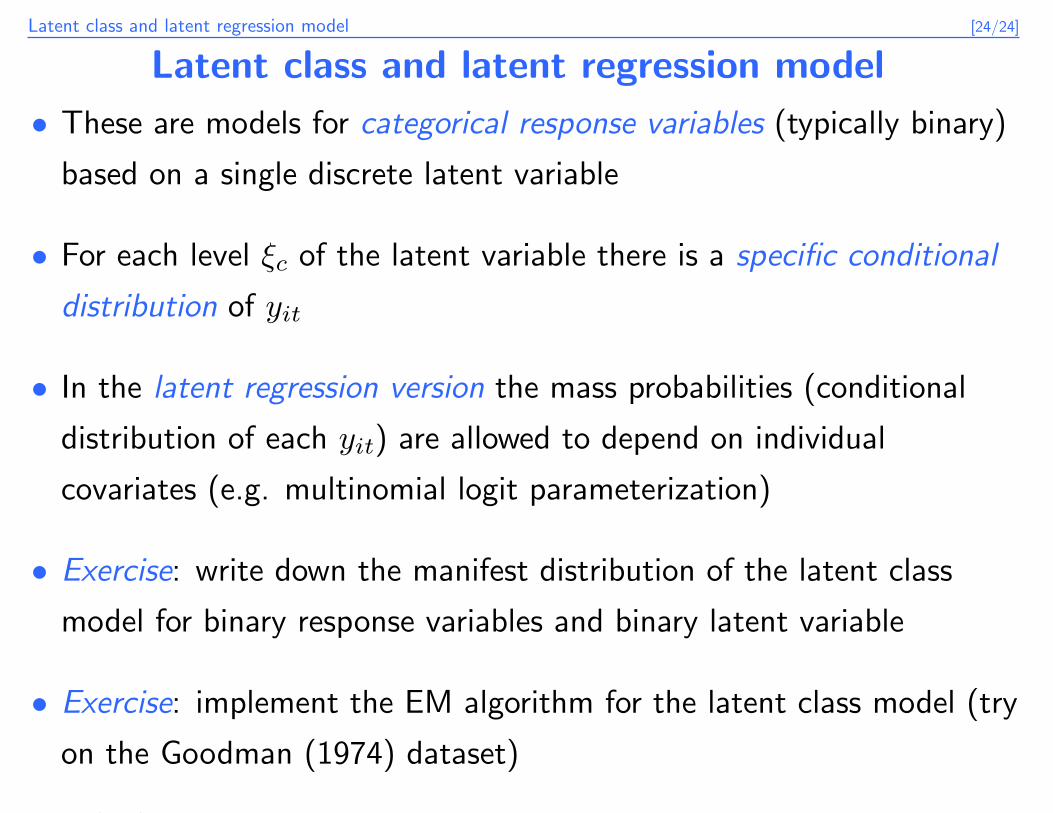
Latent class and latent regression model

• These are models for categorical response variables (typically binary)

based on a single discrete latent variable

• For each level ξc of the latent variable there is a specific conditional

distribution of yit

• In the latent regression version the mass probabilities (conditional

distribution of each yit) are allowed to depend on individual

covariates (e.g. multinomial logit parameterization)

• Exercise: write down the manifest distribution of the latent class

model for binary response variables and binary latent variable

• Exercise: implement the EM algorithm for the latent class model (try

on the Goodman (1974) dataset)



Latent regression model

• Two possible choices to include individual covariates:

1. on the measurement model so that we have random intercepts (via

a logit or probit parametrization):

λitc = p(yit = 1|ui = ξc,Xi),

logλitc

1− λitc= ξc + x

′itβ, i = 1, . . . , n, t = 1, . . . , T, c = 1, . . . , k

2. on the model for the distribution of the latent variables (via a

multinomial logit parameterization):

πic = p(ui = ξc|Xi), logπicπi1

= x′itβc, c = 2, . . . , k

• Alternative parameterizations are possible with ordinal response

variables or ordered latent classes



• The models based on the two extensions have a different

interpretation:

1. the latent variables are used to account for the unobserved

heterogeneity and then the model may be seen as discrete version

of the logistic model with one random effect

2. the main interest is on a latent variable which is measured through

the observable response variables (e.g. health status) and on how

this latent variable depends on the covariates

• Only the M-step of the EM algorithm must be modified by exploiting

standard algorithms for the maximization of:

1. the weighed likelihood of a logit model

2. the likelihood of a multinomial logit model



• Exercise: write down the manifest distribution of the latent regression

model for binary response variables and binary latent variable

• Exercise: show how to implement (and implement) the EM algorithm

for a latent class model for binary response variables (try with the

elderly people dataset)


Documents

Introduction to latent variable models - econ.upf.edumichael/latentvariables/lecture1.pdfItem Response Theory models: models for items (categorical responses) measuring a common latent