Introduction to Heegaard Floer Homology Eaman Eftekhary Harvard University Eaman Eftekhary Harvard University

Introduction to Heegaard Floer Homology

Eaman EftekharyHarvard University

Eaman EftekharyHarvard University

General ConstructionGeneral Construction

Suppose that Y is a compact oriented three-manifold equipped with a self-indexing Morse function with a unique minimum, a unique maximum, g critical points of index 1 and g critical points of index 2.

Suppose that Y is a compact oriented three-manifold equipped with a self-indexing Morse function with a unique minimum, a unique maximum, g critical points of index 1 and g critical points of index 2.

General ConstructionGeneral Construction

Suppose that Y is a compact oriented three-manifold equipped with a self-indexing Morse function h with a unique minimum, a unique maximum, g critical points of index 1 and g critical points of index 2.

The pre-image of 1.5 under h will be a surface of genus g which we denote by S.

Suppose that Y is a compact oriented three-manifold equipped with a self-indexing Morse function h with a unique minimum, a unique maximum, g critical points of index 1 and g critical points of index 2.

The pre-image of 1.5 under h will be a surface of genus g which we denote by S.

h

RR

Index 3 criticalpoint

Index 0criticalpoint

h

RR

Index 3 criticalpoint

Index 0criticalpoint

Each critical point of Index 1 or 2 willdetermine a curve

on S

h

RR

Heegaard diagrams for three-manifoldsHeegaard diagrams for three-manifolds

Each critical point of index 1 or 2 determines a simple closed curve on the surface S. Denote the curves corresponding to the index 1 critical points by i, i=1,…,g and denote the curves corresponding to the index 2 critical points by i, i=1,…,g.


Heegaard diagrams for three-manifoldsHeegaard diagrams for three-manifolds


The curves i, i=1,…,g are (homologically) linearly independent. The same is true for i, i=1,…,g.


The curves i, i=1,…,g are (homologically) linearly independent. The same is true for i, i=1,…,g.

We add a marked point z to the diagram, placed in the complement of these curves. Think of it as a flow line for the Morse function h, which connects the index 3 critical point to the index 0 critical point.


The marked point zdetermines a flow line

connecting index-0 criticalpoint to the index-3

critical point

h

RR

z


The set of data

H=(S, (1,2,…,g),(1,2,…,g),z)

is called a pointed Heegaard diagram for the three-manifold Y.


The set of data

H=(S, (1,2,…,g),(1,2,…,g),z)



The set of data

H=(S, (1,2,…,g),(1,2,…,g),z)


H uniquely determines the three-manifold Y but not vice-versa


The set of data

H=(S, (1,2,…,g),(1,2,…,g),z)


H uniquely determines the three-manifold Y but not vice-versa

A Heegaard Diagram for S1S2

Green curvesare curves andthe red ones arecurves

z

A different way of presenting this Heegaard diagram


zEach pair of circles of

the same color determines a handle



z

These arcs are completed to closed curves

using the handles

Knots in three-dimensional manifoldsKnots in three-dimensional manifolds

Any map embedding S1 in a three-manifold Y determines a homology class H1(Y,Z).

Any map embedding S1 in a three-manifold Y determines a homology class H1(Y,Z).


Any map embedding S1 to a three-manifold Y determines a homology class H1(Y,Z).

Any such map which represents the trivial homology class is called a knot.






In particular, if Y=S3, any embedding of S1 in S3 will be a knot, since the first homology of S3 is trivial.



In particular, if Y=S3, any embedding of S1 in S3 will be a knot, since the first homology of S3 is trivial.

A projection diagram for the trefoil in the

standard sphere

Trefoil in S3

Heegaard diagrams for knotsHeegaard diagrams for knots

A pair of marked points on the surface S of a Heegaard diagram H for a three-manifold Y determine a pair of paths between the critical points of indices 0 and 3. These two arcs together determine an image of S1 embedded in Y.


Heegaard diagrams for knotsHeegaard diagrams for knots


Any knot in Y may be realized in this way using some Morse function and the corresponding Heegaard diagram.


Any knot in Y may be realized in this way using some Morse function and the corresponding Heegaard diagram.

Two points on the surface S determine

a knot in Y

h

RR

z w

Heegaard diagrams for knotsHeegaard diagrams for knots A Heegaard diagram for a knot K is a set

H=(S, (1,2,…,g),(1,2,…,g),z,w)

where z,w are two marked points in the complement of the curves 1,2,…,g, and 1,2,…,g on the surface S.

A Heegaard diagram for a knot K is a set

H=(S, (1,2,…,g),(1,2,…,g),z,w)


Heegaard diagrams for knotsHeegaard diagrams for knots A Heegaard diagram for a knot K is a set

H=(S, (1,2,…,g),(1,2,…,g),z,w)


There is an arc connecting z to w in the complement of (1,2,…,g), and another arc connecting them in the complement of (1,2,…,g). Denote them by and .

A Heegaard diagram for a knot K is a set H=(S, (1,2,…,g),(1,2,…,g),z,w)


There is an arc connecting z to w in the complement of (1,2,…,g), and another arc connecting them in the complement of (1,2,…,g). Denote them by and .

Heegaard diagrams for knotsHeegaard diagrams for knots The two marked points z,w determine

the trivial homology class if and only if the closed curve - can be written as a linear combination of the curves (1,2,…,g), and (1,2,…,g) in the first homology of S.

The two marked points z,w determine the trivial homology class if and only if the closed curve - can be written as a linear combination of the curves (1,2,…,g), and (1,2,…,g) in the first homology of S.

Heegaard diagrams for knotsHeegaard diagrams for knots The two marked points z,w determine

the trivial homology class if and only if the closed curve - can be written as a linear combination of the curves (1,2,…,g), and (1,2,…,g) in the first homology of S.

The first homology group of Y may be determined from the Heegaard diagram H:

H1(Y,Z)=H1(S,Z)/[1=…= g =1=…= g=0]

The two marked points z,w determine the trivial homology class if and only if the closed curve - can be written as a linear combination of the curves (1,2,…,g), and (1,2,…,g) in the first homology of S.

The first homology group of Y may be determined from the Heegaard diagram H:

H1(Y,Z)=H1(S,Z)/[1=…= g =1=…= g=0]

A Heegaard diagram for the trefoilA Heegaard diagram for the trefoil

z

w

Constructing Heegaard diagrams for knots in S3


Consider a plane projection of a knot K in S3.





Construct a surface S by thickening this projection.







Construct a union of simple closed curves of two different colors, red and green, using the following procedure:



Construct a union of simple closed curves of two different colors, red and green, using the following procedure:

The local construction of a Heegaard diagram from a knot projection

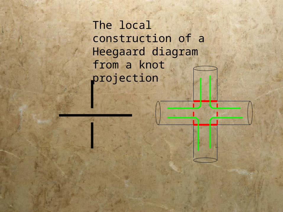
The local construction of a Heegaard diagram from a knot projection

The Heegaard diagram for trefoil after 2nd step

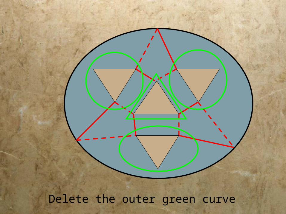
Delete the outer green curve

Add a new red curve and a pair of marked points on its twosides so that the red curve corresponds to the meridian of K.

The green curves denote 1st collection

of simple closed curves

The red curves denote 2nd collection

of simple closed curves

From topology to Heegaard diagramsFrom topology to Heegaard diagrams

Using this process we successfully extract a topological structure (a three-manifold, or a knot inside a three-manifold) from a set of combinatorial data: a marked Heegaard diagram

H=(S, (1,2,…,g),(1,2,…,g),z1,…,zn)

where n is the number of marked points on S.

Using this process we successfully extract a topological structure (a three-manifold, or a knot inside a three-manifold) from a set of combinatorial data: a marked Heegaard diagram

H=(S, (1,2,…,g),(1,2,…,g),z1,…,zn)

where n is the number of marked points on S.

From Heegaard diagrams to Floer homology


Heegaard Floer homology associates a homology theory to any Heegaard diagram with marked points.





In order to obtain an invariant of the topological structure, we should show that if two Heegaard diagrams describe the same topological structure (i.e. 3-manifold or knot), the associated homology groups are isomorphic.


In order to obtain an invariant of the topological structure, we should show that if two Heegaard diagrams describe the same topological structure (i.e. 3-manifold or knot), the associated homology groups are isomorphic.

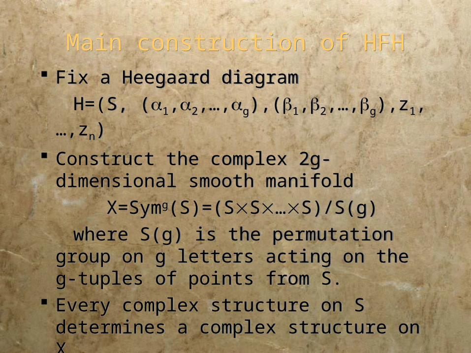
Main construction of HFHMain construction of HFH Fix a Heegaard diagram

H=(S, (1,2,…,g),(1,2,…,g),z1,…,zn)

Fix a Heegaard diagram

H=(S, (1,2,…,g),(1,2,…,g),z1,…,zn)


H=(S, (1,2,…,g),(1,2,…,g),z1,…,zn)

Construct the complex 2g-dimensional smooth manifold

X=Symg(S)=(SS…S)/S(g)

where S(g) is the permutation group on g letters acting on the g-tuples of points from S.


H=(S, (1,2,…,g),(1,2,…,g),z1,…,zn)





H=(S, (1,2,…,g),(1,2,…,g),z1,…,zn)




Every complex structure on S determines a complex structure on X.


H=(S, (1,2,…,g),(1,2,…,g),z1,…,zn)




Every complex structure on S determines a complex structure on X.

Main construction of HFHMain construction of HFH Consider the two g-dimensional tori

T=12 …g and T=12 …g

in Z=SS…S. The projection map from Z to X embeds these two tori in X.

Consider the two g-dimensional tori

T=12 …g and T=12 …g



T=12 …g and T=12 …g


These tori are totally real sub-manifolds of the complex manifold X.


T=12 …g and T=12 …g




T=12 …g and T=12 …g



If the curves 1,2,…,g meet the curves 1,2,…,g transversally on S, T will meet T transversally in X.


T=12 …g and T=12 …g



If the curves 1,2,…,g meet the curves 1,2,…,g transversally on S, T will meet T transversally in X.

Intersection points of T and T Intersection points of T and T A point of intersection between T and T

consists of a g-tuple of points (x1,x2,…,xg) such that for some element S(g) we have xii(i) for i=1,2,…,g.

A point of intersection between T and T consists of a g-tuple of points (x1,x2,…,xg) such that for some element S(g) we have xii(i) for i=1,2,…,g.

Intersection points of T and T Intersection points of T and T A point of intersection between T and T

consists of a g-tuple of points (x1,x2,…,xg) such that for some element S(g) we have xii(i) for i=1,2,…,g.

The complex CF(H), associated with the Heegaard diagram H, is generated by the intersection points x= (x1,x2,…,xg) as above.

The coefficient ring will be denoted by A,

which is a Z[u1,u2,…,un]-module.

A point of intersection between T and T consists of a g-tuple of points (x1,x2,…,xg) such that for some element S(g) we have xii(i) for i=1,2,…,g.

The complex CF(H), associated with the Heegaard diagram H, is generated by the intersection points x= (x1,x2,…,xg) as above.

The coefficient ring will be denoted by A,

which is a Z[u1,u2,…,un]-module.

Differential of the complexDifferential of the complex

The differential of this complex should have the following form:

The values b(x,y)A should be determined. Then d may be linearly extended to CF(H).

The differential of this complex should have the following form:

The values b(x,y)A should be determined. Then d may be linearly extended to CF(H).

d(x) b(x,y).yyT T

Differential of the complex; b(x,y)Differential of the complex; b(x,y) For x,y consider the space x,y

of the homotopy types of the disks satisfying the following properties:

u:[0,1]RCX

u(0,t) , u(1,t)

u(s,)=x , u(s,-)=y

For x,y consider the space x,y of the homotopy types of the disks satisfying the following properties:

u:[0,1]RCX

u(0,t) , u(1,t)

u(s,)=x , u(s,-)=y

Differential of the complex; b(x,y)Differential of the complex; b(x,y) For x,y consider the space x,y

of the homotopy types of the disks satisfying the following properties:

u:[0,1]RCX

u(0,t) , u(1,t)

u(s,)=x , u(s,-)=y

For each x,y let M() denote the moduli space of holomorphic maps u as above representing the class .

For x,y consider the space x,y of the homotopy types of the disks satisfying the following properties:

u:[0,1]RCX

u(0,t) , u(1,t)

u(s,)=x , u(s,-)=y

For each x,y let M() denote the moduli space of holomorphic maps u as above representing the class .

Differential of the complex; b(x,y)Differential of the complex; b(x,y)

u

x

y

X


There is an action of R on the moduli space M() by translation of the second component by a constant factor: If u(s,t) is holomorphic, then u(s,t+c) is also holomorphic.




If denotes the formal dimension or expected dimension of M(), then the quotient moduli space is expected to be of dimension -1. We may manage to achieve the correct dimension.


If denotes the formal dimension or expected dimension of M(), then the quotient moduli space is expected to be of dimension -1. We may manage to achieve the correct dimension.


Let n( denote the number of points in the quotient moduli space (counted with a sign) if =1. Otherwise define n(=0.




Let n(j, denote the intersection number

of L(zj)={zj}Symg-1(S) Symg(S)=X

with .




with .





with .

Define b(x,y)=∑ n(.∏j uj n(j,

where the sum is over all x,y.




with .

Define b(x,y)=∑ n(.∏j uj n(j,

where the sum is over all x,y.

Two examples in dimension twoTwo examples in dimension two

x

y

Example 1.


x

y

There is a unique holomorphic Disk, up to reparametrization

of the domain, by RiemannMapping theorem

Example 1.


x

y

Example 1.

d(x)=y


x

y

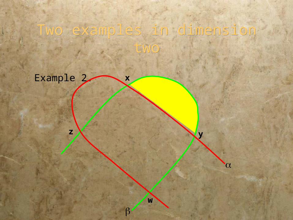
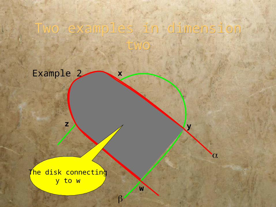
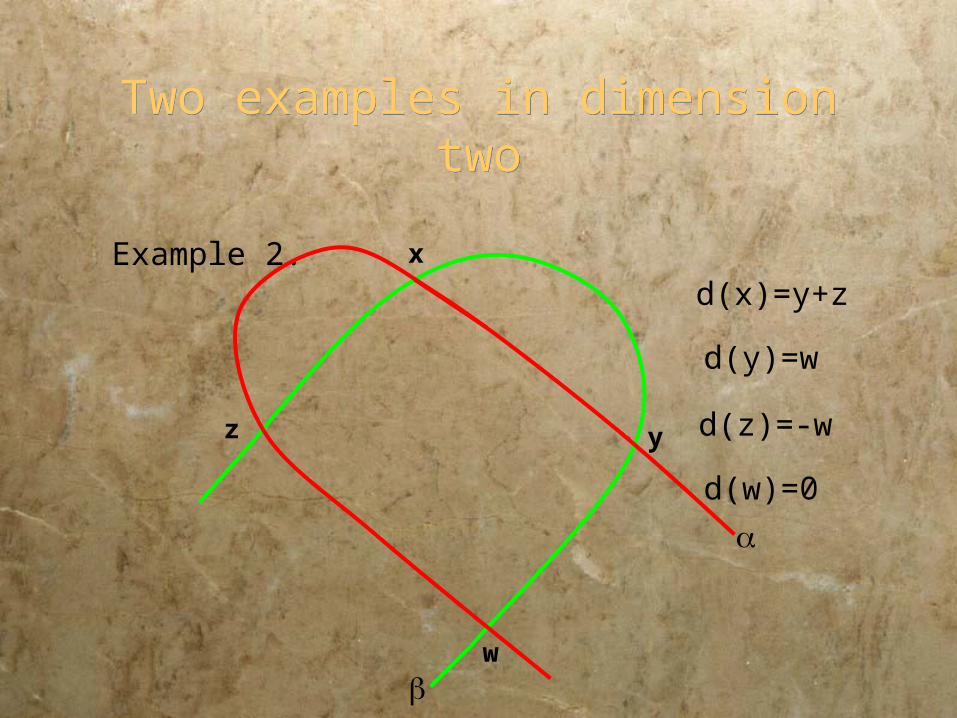
Example 2.

w

z


x

y

There is a unique holomorphic disk from x to y, up to reparametrization

of the domain, by RiemannMapping theorem

Example 2.

w

z


x

y

Example 2.

w

z


x

y

Example 2.

w

z

The disk connecting x to z


x

y

Example 2.

w

z

The disk connectingz to w


x

y

Example 2.

w

z

The disk connectingy to w


x

y

Example 2.

w

z


x

y

Example 2.

w

z

There is a one parameterfamily of disks connecting x to

y parameterized by thelength of the cut


x

y

Example 2.

w

z

d(x)=y+z

d(y)=w

d(z)=-w

d(w)=0

Basic properties Basic properties The first observation is that d2=0. The first observation is that d2=0.

Basic properties Basic properties The first observation is that d2=0. This may be checked easily in the two

examples discussed here.

The first observation is that d2=0. This may be checked easily in the two

examples discussed here.

Basic properties Basic properties The first observation is that d2=0. This may be checked easily in the two

examples discussed here. In general the proof uses a description

of the boundary of M/~ when . Here ~ denotes the equivalence relation obtained by R-translation. Gromov compactness theorem and a gluing lemma should be used.

The first observation is that d2=0. This may be checked easily in the two

examples discussed here. In general the proof uses a description

of the boundary of M/~ when . Here ~ denotes the equivalence relation obtained by R-translation. Gromov compactness theorem and a gluing lemma should be used.

Basic properties Basic properties

Theorem (Ozsváth-Szabó) The homology groups HF(H,A) of the complex (CF(H),d) are invariants of the pointed Heegaard diagram H. For a three-manifold Y, or a knot (KY), the homology group is in fact independent of the specific Heegaard diagram used for constructing the chain complex and gives homology groups HF(Y,A) and HFK(K,A) respectively.

Theorem (Ozsváth-Szabó) The homology groups HF(H,A) of the complex (CF(H),d) are invariants of the pointed Heegaard diagram H. For a three-manifold Y, or a knot (KY), the homology group is in fact independent of the specific Heegaard diagram used for constructing the chain complex and gives homology groups HF(Y,A) and HFK(K,A) respectively.

Refinements of these homology groups Refinements of these homology groups Consider the space Spinc(Y) of Spinc-

structures on Y. This is the space of homology classes of nowhere vanishing vector fields on Y. Two non-vanishing vector fields on Y are called homologous if they are isotopic in the complement of a ball in Y.

Consider the space Spinc(Y) of Spinc-structures on Y. This is the space of homology classes of nowhere vanishing vector fields on Y. Two non-vanishing vector fields on Y are called homologous if they are isotopic in the complement of a ball in Y.

Refinements of these homology groups Refinements of these homology groups Consider the space Spinc(Y) of Spinc-

structures on Y. This is the space of homology classes of nowhere vanishing vector fields on Y. Two non-vanishing vector fields on Y are called homologous if they are isotopic in the complement of a ball in Y.

The marked point z defines a map sz from the set of generators of CF(H) to Spinc(Y):

sz:Spinc(Y) defined as follows

Consider the space Spinc(Y) of Spinc-structures on Y. This is the space of homology classes of nowhere vanishing vector fields on Y. Two non-vanishing vector fields on Y are called homologous if they are isotopic in the complement of a ball in Y.

The marked point z defines a map sz from the set of generators of CF(H) to Spinc(Y):

sz:Spinc(Y) defined as follows

Refinements of these homology groups Refinements of these homology groups If x=(x1,x2,…,xg) is an intersection

point, then each of xj determines a flow line for the Morse function h connecting one of the index-1 critical points to an index-2 critical point. The marked point z determines a flow line connecting the index-0 critical point to the index-3 critical point.

If x=(x1,x2,…,xg) is an intersection point, then each of xj determines a flow line for the Morse function h connecting one of the index-1 critical points to an index-2 critical point. The marked point z determines a flow line connecting the index-0 critical point to the index-3 critical point.

Refinements of these homology groups Refinements of these homology groups If x=(x1,x2,…,xg) is an intersection

point, then each of xj determines a flow line for the Morse function h connecting one of the index-1 critical points to an index-2 critical point. The marked point z determines a flow line connecting the index-0 critical point to the index-3 critical point.

All together we obtain a union of flow lines joining pairs of critical points of indices of different parity.

If x=(x1,x2,…,xg) is an intersection point, then each of xj determines a flow line for the Morse function h connecting one of the index-1 critical points to an index-2 critical point. The marked point z determines a flow line connecting the index-0 critical point to the index-3 critical point.

All together we obtain a union of flow lines joining pairs of critical points of indices of different parity.

Refinements of these homology

groups Refinements of these homology

groups The gradient vector field may be modified

in a neighborhood of these paths to obtain a nowhere vanishing vector field on Y.

The gradient vector field may be modified in a neighborhood of these paths to obtain a nowhere vanishing vector field on Y.





The class of this vector field in Spinc(Y) is independent of this modification and is denoted by sz(x).








If x,y are intersection points with

x,y, then sz(x) =sz(y).



If x,y are intersection points with

x,y, then sz(x) =sz(y).



groups This implies that the homology groups

HF(Y,A) decompose according to the Spinc structures over Y:

HF(Y,A)=sSpin(Y)HF(Y,A;s)

This implies that the homology groups HF(Y,A) decompose according to the Spinc structures over Y:




groups This implies that the homology groups

HF(Y,A) decompose according to the Spinc structures over Y:


For each sSpinc(Y) the group HF(Y,A;s) is also an invariant of the three-manifold Y and the Spinc structure s.

This implies that the homology groups HF(Y,A) decompose according to the Spinc structures over Y:


For each sSpinc(Y) the group HF(Y,A;s) is also an invariant of the three-manifold Y and the Spinc structure s.

Some examplesSome examples

For S3, Spinc(S3)={s0} and HF(Y,A;s0)=A For S3, Spinc(S3)={s0} and HF(Y,A;s0)=A

Some examplesSome examples

For S3, Spinc(S3)={s0} and HF(Y,A;s0)=A

For S1S2, Spinc(S1S2)=Z. Let s0 be the Spinc structure such that c1(s0)=0, then for s≠s0, HF(Y,A;s)=0. Furthermore we have HF(Y,A;s0)=AA, where the homological gradings of the two copies of A differ by 1.

For S3, Spinc(S3)={s0} and HF(Y,A;s0)=A

For S1S2, Spinc(S1S2)=Z. Let s0 be the Spinc structure such that c1(s0)=0, then for s≠s0, HF(Y,A;s)=0. Furthermore we have HF(Y,A;s0)=AA, where the homological gradings of the two copies of A differ by 1.

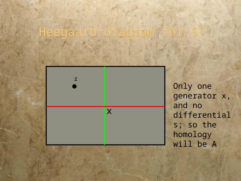
Heegaard diagram for S3Heegaard diagram for S3

z

x

The opposite sides of the rectangle should be identified to obtain a torus (surface of genus1)

Heegaard diagram for S3Heegaard diagram for S3

z

x

Only one generator x, and no differentials; so the homology will be A

Heegaard diagram for S1S2Heegaard diagram for S1S2

z

x

Only two generators x,y and two homotopy classes of disks of index 1.

y


z

x

The first disk connecting x to y, with Maslov index one.

y


z

x

The second disk connecting x to y, with Maslov index one. The sign will be different from the first one.

y


z

x

d(x)=d(y)=0sz(x)=sz(y)=s0

(x)=(y)+1=1HF(S1S2,A,s0)=AxAy

y

Some other simple casesSome other simple cases

Lens spaces L(p,q) Lens spaces L(p,q)


Lens spaces L(p,q) S3

n(K): the result of n-surgery on alternating knots in S3. The result may be understood in terms of the Alexander polynomial of the knot.






Connected sums of pieces of the above type: There is a connected sum formula.



Connected sums of pieces of the above type: There is a connected sum formula.

Connected sum formulaConnected sum formula

Spinc(Y1#Y2)=Spinc(Y1)Spinc(Y2); Maybe the better notation is Spinc(Y1#Y2)=Spinc(Y1)#Spinc(Y2)




HF(Y1#Y2,A;s1#s2)=

HF(Y1,A;s1)AHF(Y2,A;s2)


HF(Y1#Y2,A;s1#s2)=




HF(Y1#Y2,A;s1#s2)=


In particular for A=Z, as a trivial Z[u1]-module, the connected sum formula is usually simple (in practice).


HF(Y1#Y2,A;s1#s2)=


In particular for A=Z, as a trivial Z[u1]-module, the connected sum formula is usually simple (in practice).

Refinements for knotsRefinements for knots

Consider the space of relative Spinc structures Spinc(Y,K) for a knot (Y,K);




Spinc(Y,K) is by definition the space of homology classes of non-vanishing vector fields in the complement of K which converge to the orientation of K.


Spinc(Y,K) is by definition the space of homology classes of non-vanishing vector fields in the complement of K which converge to the orientation of K.


The pair of marked points (z,w) on a Heegaard diagram H for K determine a map from the set of generators x to Spinc(Y,K), denoted by sK(x) Spinc(Y,K).




In the simplest case where A=Z, the coefficient of any y in d(x) is zero, unless sK(x)=sK(y).


In the simplest case where A=Z, the coefficient of any y in d(x) is zero, unless sK(x)=sK(y).


This is a better refinement in comparison with the previous one for three-manifolds:

Spinc(Y,K)=ZSpinc(Y)


Spinc(Y,K)=ZSpinc(Y)



Spinc(Y,K)=ZSpinc(Y) In particular for Y=S3 and standard knots

we have Spinc(K):=Spinc(S3,K)=Z We restrict ourselves to this case, with

A=Z!


Spinc(Y,K)=ZSpinc(Y) In particular for Y=S3 and standard knots

we have Spinc(K):=Spinc(S3,K)=Z We restrict ourselves to this case, with

A=Z!

Some results for knots in S3Some results for knots in S3

For each sZ, we obtain a homology group HF(K,s) which is an invariant for K.




There is a homological grading induced on HF(K,s). As a result

HF(K,s)=iZ HFi(K,s)



HF(K,s)=iZ HFi(K,s)




HF(K,s)=iZ HFi(K,s)

So each HF(K,s) has a well-defined Euler characteristic (K,s)



HF(K,s)=iZ HFi(K,s)

So each HF(K,s) has a well-defined Euler characteristic (K,s)


The polynomial

PK(t)=∑sZ (K,s).ts

will be the symmetrized Alexander polynomial of K.

The polynomial




The polynomial



There is a symmetry as follows:

HFi(K,s)=HFi-2s(K,-s)

The polynomial






The polynomial





HF(K) determines the genus of K as follows;

The polynomial





HF(K) determines the genus of K as follows;

Genus of a knotGenus of a knot

Suppose that K is a knot in S3. Suppose that K is a knot in S3.


Suppose that K is a knot in S3. Consider all the oriented surfaces C

with one boundary component in S3\K such that the boundary of C is K.






Such a surface is called a Seifert surface for K.








The genus g(K) of K is the minimum genus for a Seifert surface for K.




The genus g(K) of K is the minimum genus for a Seifert surface for K.

HFH determines the genusHFH determines the genus

Let d(K) be the largest integer s such that HF(K,s) is non-trivial.


HFH determines the genusHFH determines the genus


Theorem (Ozsváth-Szabó) For any knot K in S3, d(K)=g(K).


Theorem (Ozsváth-Szabó) For any knot K in S3, d(K)=g(K).

HFH and the 4-ball genusHFH and the 4-ball genus

In fact there is a slightly more interesting invariant (K) defined from HF(K,A), where A=Z[u1

-1,u2-1], which gives a lower

bound for the 4-ball genus g4(K) of K.








The 4-ball genus in the smallest genus of a surface in the 4-ball with boundary K in S3, which is the boundary of the 4-ball.




The 4-ball genus in the smallest genus of a surface in the 4-ball with boundary K in S3, which is the boundary of the 4-ball.


The 4-ball genus gives a lower bound for the un-knotting number u(K) of K.




Theorem(Ozsváth-Szabó)

(K) ≤g4(K)≤u(K)



(K) ≤g4(K)≤u(K)




(K) ≤g4(K)≤u(K)

Corollary(Milnor conjecture, 1st proved by Kronheimer-Mrowka using gauge theory)

If T(p,q) denotes the (p,q) torus knot, then u(T(p,q))=(p-1)(q-1)/2



(K) ≤g4(K)≤u(K)

Corollary(Milnor conjecture, 1st proved by Kronheimer-Mrowka using gauge theory)

If T(p,q) denotes the (p,q) torus knot, then u(T(p,q))=(p-1)(q-1)/2

T(p,q): p strands, q twistsT(p,q): p strands, q twists

CompationsCompations

HF(K) is completely determined from the symmetrized Alexander polynomial and the signature (K), if K is an alternating knot.




Torus knots, three-strand pretzel knots, etc.






Small knots: We know the answer for all knots up to 14 crossings.



Small knots: We know the answer for all knots up to 14 crossings.

Why is it possible to compute?Why is it possible to compute?

There is an easy way to understand the homotopy classes of disks in x,y) when the associated relative Spinc structures associated with x,y in Spinc(K) are the same.




Let be an element in x,y), and let z1,z2,…,zm be marked points on S, one in each connected component of the complement of the curves in S.


Let be an element in x,y), and let z1,z2,…,zm be marked points on S, one in each connected component of the complement of the curves in S.


Consider the subspaces L(zj)={zj}Symg-1(S) and let n(j,) be the intersection number of with L(zj).




The collection of integers n(j,), j=1,…,m determine the homotopy class .






There is a simple combinatorial way to check if such a collection determines a homotopy class in x,y) or not.



There is a simple combinatorial way to check if such a collection determines a homotopy class in x,y) or not.


There is a combinatorial formula for the expected dimension of of M() in terms of n(j,) and the geometry of the curves on S.




We know that if n() is not zero, then =1, and all n(j,) are non-negative. Furthermore, if z=z1 and w=z2, then n(1,)= n(2,)=0.


We know that if n() is not zero, then =1, and all n(j,) are non-negative. Furthermore, if z=z1 and w=z2, then n(1,)= n(2,)=0.


These are strong restrictions. For example these restrictions are enough for a complete computation for alternating knots.




In other cases, these are still pretty strong, and help a lot with the computations.






There are computer programs (e.g. by Monalescue) which provide all the simplifications of the above type in the computations.



There are computer programs (e.g. by Monalescue) which provide all the simplifications of the above type in the computations.

Some domains for which the moduli space is known


x

y

y

y

x

x

Any 2n-gone as shown here with alternating red and green edges corresponds to as moduli space contributing 1 to the differential



x

y

y

y

x

x

The same is true for thesame type of polygons witha number of circles excluded as shown in the picture.x=y

Relation to the three-manifold invariants


Theorem (Ozsváth-Szabó) Heegaard Floer complex for a knot K determines the Heegaard Floer homology for three-manifolds obtained by surgery on K.

Theorem (Ozsváth-Szabó) Heegaard Floer complex for a knot K determines the Heegaard Floer homology for three-manifolds obtained by surgery on K.



Theorem (E.) More generally if a 3-manifold is obtained from two knot-complements by identifying them on the boundary, then the Heegaard Floer complexs of the two knots, determine the Heegaard Floer homology of the resulting three-manifold

Theorem (E.) More generally if a 3-manifold is obtained from two knot-complements by identifying them on the boundary, then the Heegaard Floer complexs of the two knots, determine the Heegaard Floer homology of the resulting three-manifold

Documents

Introduction to Heegaard Floer Homology Eaman Eftekhary Harvard University Eaman Eftekhary Harvard University