CHAPTER 4 INTRODUCTION TO GREEN’S FUNCTION

Green's functions are named after the mathematician, George

Green, who first developed the concept in the 1830s. In the modern study

of linear partial differential equations, Green's functions are studied

largely from the point of view of fundamental solutions instead. It is an

important mathematical tool that has application in many areas of

theoretical physics including mechanics, electromagnetism, solid-state

physics, thermal physics, and the theory of elementary particles. For the

solution of Boundary value problems associated with either ordinary or

partial differential equations, one requires a brief knowledge about

Green's function . Unfortunately it took many years to emerge from the

realms of more formal and abstract mathematical analysis as a potential

everyday tool for the practical study of Boundary value problem.

4.1 FUNDAMENTAL CONCEPT

Initially we solve, by fairly elementary methods, a typical one

dimensional boundary value problem for the understanding of Green’s

function.

Consider the differential equation,

)()( xfxuL (4.1.1)

where L is an ordinary linear differential operator, )(xf is a known

function while )(xu is an unknown function. To solve above equation, one

48

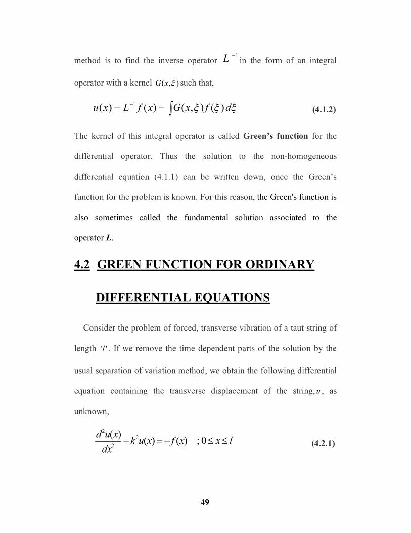
method is to find the inverse operator 1L in the form of an integral

operator with a kernel ),( xG such that,

dfxGxfLxu )(),()()( 1 (4.1.2)

The kernel of this integral operator is called Green’s function for the

differential operator. Thus the solution to the non-homogeneous

differential equation (4.1.1) can be written down, once the Green’s

function for the problem is known. For this reason, the Green's function is

also sometimes called the fundamental solution associated to the

operator L.

4.2 GREEN FUNCTION FOR ORDINARY

DIFFERENTIAL EQUATIONS

Consider the problem of forced, transverse vibration of a taut string of

length ''l . If we remove the time dependent parts of the solution by the

usual separation of variation method, we obtain the following differential

equation containing the transverse displacement of the string, u , as

unknown,

lxxfxukdx

xud 0;)()()( 2

2

2

(4.2.1)

49

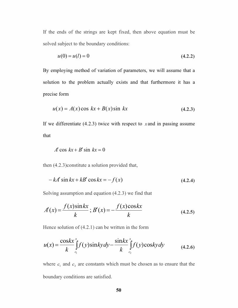
If the ends of the strings are kept fixed, then above equation must be

solved subject to the boundary conditions:

0)()0( luu (4.2.2)

By employing method of variation of parameters, we will assume that a

solution to the problem actually exists and that furthermore it has a

precise form

kxxBkxxAxu sin)(cos)()( (4.2.3)

If we differentiate (4.2.3) twice with respect to x and in passing assume

that

0sincos kxBkxA

then (4.2.3)constitute a solution provided that,

)(cossin xfkxBkkxAk (4.2.4)

Solving assumption and equation (4.2.3) we find that

kkxxfxB

kkxxfxA cos)()(;sin)()( (4.2.5)

Hence solution of (4.2.1) can be written in the form

dykyyfkkxdykyyf

kkxxu

x

c

x

c

cos)(sinsin)(cos)(21

(4.2.6)

where 1c and 2c are constants which must be chosen as to ensure that the

boundary conditions are satisfied.

50

Inserting BC; 0)0( u

We find that we must choose 1c such that

00sin)( 1

0

1

cdykyyfc

(4.2.7)

Hence (4.2.6) reduces to

dykyyfkkxdykyyf

kkxxu

x

c

x

cos)(sinsin)(cos)(20 (4.2.8)

which imply we must choose 01 c

Using second BC in (4.2.8) we have

dykyyfklkldykyyf

ll

c

sin)(sincoscos)(

02

(4.2.9)

After slight manipulation we can re write the above equation as

dyklkyklkyyfkl

dykyyfl

c

]sincoscos[sin)(sin

1cos)(0

0

2

dylykyfkl

dykyyfl

c

)]([sin)(sin

1cos)(0

0

2

(4.2.10)

Solution can now be written in the form

dylykyfklk

kx

dykyyfk

kxdykyyfk

kxxu

l

xx

)(sin)(sin

sin

cos)(sinsin)(cos)(

0

00

51

= dyklk

ylkkxyfdyklk

xykklyfl

x

x

sin)(sinsin)(

sin)(sinsin)(

0

= dyyxGyfl

),()(0 (4.2.11)

where ),( yxG can be introduced as,

),( yxG = xylkk

xlkyk

0;

sin)(sinsin

= lyxlkk

ylkxk

;sin

)(sinsin

This function ),( yxG is a two point function of position, known as the

Green’s function for the equation (4.2.1) and the boundary conditions. Its

existence is assured, provided 0sin kl . Thus we see that when

),( yxG exists and when it is known explicitly then we can immediately

write down the solution to our boundary value problem along with given

boundary conditions. One of the main advantages of above expressed

Green function is that it is independent of the Forcing term )(xf and

depends only upon the particular differential equation along with

boundary conditions imposed. Once ),( yxG has been determined; always

provided that the resulting integral in (4.2.11) exists.

Before extending the concept of Green’s Function to the parabolic

equations some basic concepts that are utilized in the solution have to be

explored.

52

4.3 CONCEPT OF EIGEN VALUES AND

EIGEN FUNCTIONS

Let )(x satisfy a second order ordinary differential equations with two

homogeneous boundary conditions:

0)(0)0(

2

2

L

xdd

(4.3.1)

It is a boundary value problem, since the two conditions are not

given at the same place, but at the two different places, 0x and Lx .

There is no simple theory which guarantees that the solution exists or is

unique to this type of problem. In particular, we note that 0)( x satisfies

the ODE and both homogeneous boundary conditions, no matter what the

separation constant is, even if < 0, it is referred to as the trivial

solution of the boundary value problem. It corresponds to 0),( txu ,

where )()(),( tGxtxu . If the solution of given problem had been

unique, then 0)( x would be the only solution; we would not be able to

obtain a nontrivial solutions of linear homogeneous PDE by separation of

variables method.

Fortunately there are other solutions. However, there do not exist a

non trivial solution for all values of . Instead we will show that there

53

are certain special values of , called eigen values of the given

boundary value problem for which there are non-trivial solutions, )(x .

A non-trivial )(x , which exists for certain values of , is known as

eigen functions corresponds to the eigen value .

For the determination of eigen value of given problem, we observe

that the given equation is linear and homogeneous with constant

coefficients; two independent solutions are usually obtained in the form

of exponentials; )exp()( xrx . Substituting this into the differential

equation yields the characteristic polynomial 2r .The solutions

corresponding to two roots have significantly different properties

depending on the values of .

Case:1 0

In this case exponential solutions have imaginary exponents

)exp( xi and solution oscillates. For real solutions we can choose

xcos and xsin in general.

Thus general solution in this case is :

xCxCx sincos)( 21 (4.3.2)

Boundary condition at 0x 01 C

so xCx sin)( 2

54

Then boundary condition at

Lx 0sin2 LC

either 02 C or 0sin L .

If 02 C then 0)( x , this is a trivial solution.

Now nLL 0sin

We are searching for those values of that have non-trivial

solutions, therefore eigen value must satisfy

0sin x .

,...3,2,12

n

Ln

Hence the eigen vector corresponding to eigen value is

LxnCx sin)( 2

where 2C is an arbitrary constant.

Case:2 0

In this case xCCx 21)(

corresponding to double zero roots; r =0 of the characteristic polynomial.

Boundary condition at 0x 01 C

55

then boundary condition at Lx 02 LC .

Since length L is positive this gives a trivial solution 0)( x .

Thus 0 is not an eigen value for the problem.

Case:3 0

In this case the roots of the characteristic polynomials are

r , so solutions are )exp( x and )exp( x . We may

prefer equivalent notation .

Considering 0 and suppose S , gives 0S

Therefore we have

)exp()exp()( 21 xSCxSCx

In terms of Hyperbolic function this can be rewritten as

)(sinh)(cosh)( 43 xSCxSCx

Boundary condition at 0x 03 C

Then, boundary condition at Lx 0)(sinh4 LSC .

Since 0LS and since sinh is never zero for a positive argument, it

follows that 0 C4 . 0 )x( .

The only solution to (4.3.2) for 0 that solves the homogeneous

boundary conditions is the trivial solution.

56

4.4 METHOD OF EIGEN FUNCTION

EXPANSION

Consider a problem of non homogeneous linear partial differential

equation with homogeneous boundary conditions.

)()0,(

0),0(;0),0(

),(2

2

xgxvLvtv

txQx

vktv

(4.4.1)

Now related Homogeneous problem is given by

0),0(;0),0(

2

2

Lutu

xuk

tu

(4.4.2)

the eigen functions of related homogeneous problem satisfy

0)(0)0(

2

2

L

xdd

Now from above discussion we know that the eigen values are

,...3,2,12

n

Ln and the corresponding eigen functions are

Lxnxn sin)( which are known.

57

The method of eigen function expansion, employed to solve the non

homogeneous problem with homogeneous boundary conditions consists

in expanding the unknown solution ),( txv in a series of the related

homogeneous eigen functions:

)()(),(1

xtatxv nn

n

(4.4.3)

For each fixed t , ),( txv is a function of x , and hence ),( txv will have

a generalized Fourier series.

In this case we have an ordinary Fourier sine series, and

generalized Fourier coefficients are na ,which varies as t changes. Here

)(tan are not the time dependent separated solutions tLnke2)( but

they are just generalized Fourier coefficients for ),( txv which can be

determined as follows

Orthogonality of Sines :

Let,

Lxnaxgxv

nn

sin)()0,(1

(4.4.4)

We will assume that standard mathematical operations are also valid for

infinite series. Equation represents one equation in an infinite number of

unknowns but it should be valid at every value of x . If we substitute a

thousand different values of x into above equation, each of the thousand

58

equations would hold, but there would still be an infinite number of

unknowns. This is not an efficient way to determine na . Instead, we

frequently will employ an extremely important technique based on

noticing that the eigen functions L

xnsin satisfying the following integral

property.

(4.4.5(b)) n m ; L/2 (4.4.5(a)) n m ; 0

dx L

xmsin L

xnsin L

0

where m and n are positive integers.

To use this conditions (4.4.5) to determine na , we multiply both

sides of (4.4.4) by L

xmsin ( for any fixed integer m, independent of the

‘dummy’ index n).

))(sin(sinsin)(1 L

xmL

xnaL

xmxgn

n

Now we integrate with respect to x , from x = 0 to x = L :

dxL

xmL

xnadxL

xmxgn

l

n

L

1 00

))(sin(sinsin)(

For finite series the integral of a sum of terms equals the sum of

integrals. We assume that this is valid for this infinite series. Now we

evaluate the infinite sum. From the integral property (4.4.5) we see that

each term of the sum is zero whenever m n . In summing over n,

59

eventually n equals m. It is only for that one value of n ( n = m ) that

there is a contribution to the infinite sum. The only term that appears on

the right hand side of occurs when n is replaced by m :

dxL

xmadxL

xmxgL

m

L

0

2

0

sinsin)(

Since the integral on the right equals L/2, we can solve for na :

dxL

xnxgLdx

Lxm

dxL

xmxga

L

L

L

m

sin)(2

sin

sin)(

02

0

0

(4.4.6)

The integral in (4.4.6) is considered to be known since x)(g is the given

initial condition.

4.5 GREEN FUNCTIONS FOR PARABOLIC

DIFFERENTIAL EQUATION

A concept of Green’s Function method now can be extended to a

parabolic equation and its associated boundary value problem for brief

understanding.

Consider a problem associated with the Diffusion equation:

tuu

2 (4.5.1)(a)

60

which holds through out a finite, bounded region D. The boundary

conditions imposed on the solution function u, is taken to be,

DPPfPutallforDptpu

)()0,(,0),(

(4.5.1)(b)

Where second equation represent the initial distribution of u throughout D

consequently a “boundary value problem” for a parabolic equation can be

typified as:

DPtuPu

)(2

DPPfPu

tallforDptpu

)()0,(,0),(

(4.5.2)

For solution of such problem we assume an expansion for the solution

function, u, in the form,

)()(),(1

PutctPu nn

n

(4.5.3)

where )(tcn is an undetermined function of t and the functions nu are

orthonormal eigen functions, with corresponding eigen values n defined

by the problem:

DPPvDPPvPv 0)(;0)()(2 (4.5.4)

Employing orthonormality property of the eigen function nu , we obtain

from (4.5.3),

61

PnDn dPutPutc )(),()( (4.5.5)

Differentiating with respect to time we have,

PnD

PnDn

dPutPu

dPutPutc

)(),(

)(),()(2

Applying Green’s identity to ),( tPu and )(Pun throughout the region D,

and implementing the boundary conditions imposed on the functions we

can write:

PnD

PnDn

dPutPu

dPutPutc

)(),(

)(),()(2

2

)()( tctc nnn

The solution for this first order Ordinary differential equation for )(tcn is:

)exp()0()( tctc nnn (4.5.6)

Imposing Initial conditions on ),( tPu we find ,

D Pnnn dPuPffc )()()0( (4.5.7)

substituting (4.5.6) and (4.5.7) in (4.5.3) we obtain

Qnn

nnD

QnDnn

n

dQuPutQf

dQuQfPuttPu

)()()exp()(

)()()()exp(),(

1

1

which gives

62

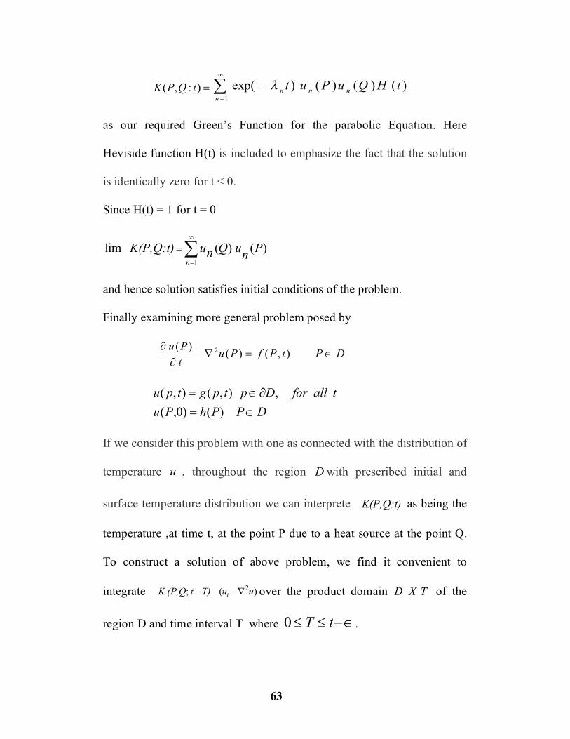
):,( tQPK )()()()exp(1

tHQuPut nnn

n

as our required Green’s Function for the parabolic Equation. Here

Heviside function H(t) is included to emphasize the fact that the solution

is identically zero for t < 0.

Since H(t) = 1 for t = 0

)()(lim1

PnuQnu K(P,Q:t)n

and hence solution satisfies initial conditions of the problem.

Finally examining more general problem posed by

DPtPfPutPu

),()()( 2

DPPhPutallforDptpgtpu

)()0,(,),(),(

If we consider this problem with one as connected with the distribution of

temperature u , throughout the region D with prescribed initial and

surface temperature distribution we can interprete K(P,Q:t) as being the

temperature ,at time t, at the point P due to a heat source at the point Q.

To construct a solution of above problem, we find it convenient to

integrate )(; 2uuT)t(P,Q K t over the product domain XD T of the

region D and time interval T where tT0 .

63

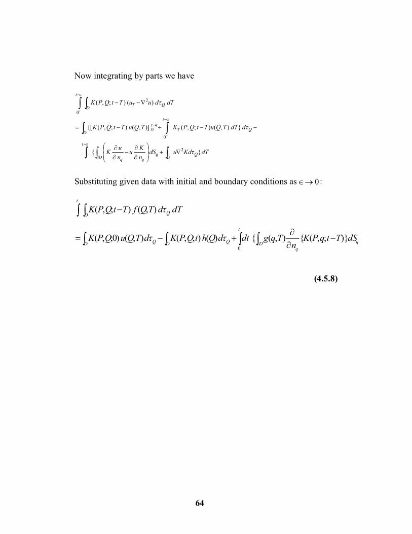
Now integrating by parts we have

dTKdudSnKu

nuK

ddTTQuTtQPKTQuTtQPK

dTduuTtQPK

QD

qD qq

t

QT

tt

D

QT

t

D

}{

}),();,()],();,({[

)();,(

2

0

0

2

0

Substituting given data with initial and boundary conditions as 0 :

qDq

t

QDQD

Q

t

D

dSTtqPKn

TqgdtdQhtQPKdTQuQPK

dTdTQfTtQPK

)};,({),({)();,(),()0;,(

),();,(

0

(4.5.8)

64