Embed Size (px)
Citation preview
Introduction to genetic Introduction to genetic network modelsnetwork models
Roberto Serra
Centro Ricerche Ambientali Montecatini
why networks basics of gene regulation generic properties self-organizing dynamical systems the Kauffman model continuous models topology of complex networks small world networks
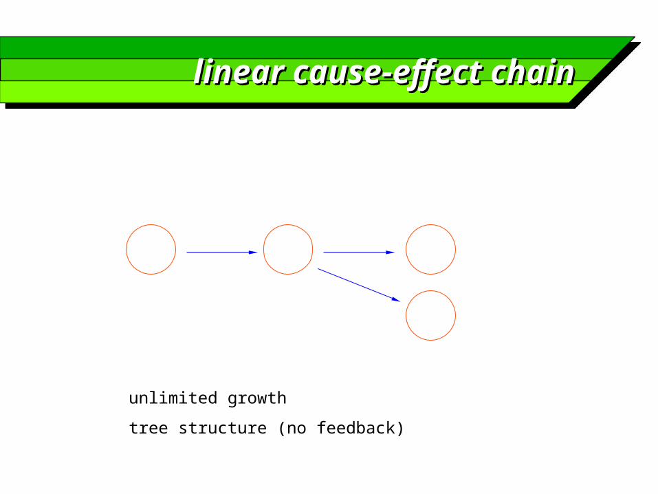
linear cause-effect chainlinear cause-effect chain
unlimited growth
tree structure (no feedback)
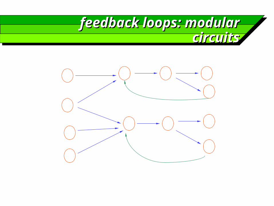
feedback loops: modular feedback loops: modular circuitscircuits

web of interacting circuitsweb of interacting circuits

not only genesnot only genes
chemicals
proteinsgenes
from outside
synthesis
regulation
activation
catalysis

control pointscontrol points
DNA primary RNA transcript
mRNAmRNA-ribosome
transcriptionalcontrol
RNA processing
protein
mRNA transport mRNA degradation
translational control
protein activity control

cis- and trans-acting controlcis- and trans-acting control

control mechanismscontrol mechanisms
the most effective regulation acts at transcription level RNAp binds to a DNA region upstream of the coding
region, the promoter regulatory proteins can “recognize” certain sequences
and bind to them the interactions between proteins and segments of the
DNA chain are highly specific proteins recognize specificic sequences of bases
without the need for opening the DNA double helix in eucaryotes it is necessary the the DNA molecule be
unbound in order for the regulatory proteins to operate

product inhibitionproduct inhibition
bound RNAp
inactive repressor
repressor activated by tryptophan

catabolite induced activationcatabolite induced activation
inactive CAP
CAP activated by cAMP

collective regulatory collective regulatory mechanismsmechanisms
groups of genes may be activated or inactivated simoultaneously
sigma factors in bacteria transcription factors in eucaryotes
these mechanism introduce correlations among the expression patterns of different genes
certain kinds of packaging of genes in eucaryotes (e.g. heterochromatin) make genes in that region inaccessible to RNAp

modelling levelmodelling level
the choice of the modelling level is a crucial step while there are detailed models of the protein synthesis process, in
order to understand network properties it is advisable to use a simplified view of the synthesis
activation level of a given gene = concentration of the corresponding mRNA concentration of the corresponding protein
concentrations can be expressed either as continuous or as discrete variables
the latter when there are say a few molecules per cell
a boolean approximation may often be appropriately employed
our “standard” choice: activation = concentration of the corresponding protein activation = continuous or boolean

asking specific questionsasking specific questions
modelling specific control circuits which genes, chemicals etc. directly affect the
expression of my-gene? or which do affect it in an indirect way ? which are the control regions? which interactions are there among the control
molecules, which is the logic of the control? these are “classical” problems in biological research on
genetic control provide detailed, specific information about specific
circuits which serve as a guide to guess the general principles
of network “design”
a complementary approacha complementary approach
trying to understand the properties of large networks if we knew all the details, we could write down the exact
model of the overall network but this is impossible so far looking at general properties of “networks of the kind”
which is present in cells general properties means global structural features,
types of possible dynamical behaviours, etc. this analysis has very strong implications for the theory of biological
evolution
the search for generic properties may also provide hints for the analysis of specific circuits
which questions to ask which features to expect
generic properties of genetic generic properties of genetic networksnetworks
the strategy: analyze ensembles of networks
the ensemble is composed by networks which share some overall features (constraints)
nonconstrained features vary at random in the ensemble
characterize the statistical distribution
analyze the generic features
ensembles of networksensembles of networks
a technique from statistical physics example: the Hopfield model of boolean neural
networks stored patterns are “memorized” in a set of weights W wij weight connecting nodes i and j every set of stored patterns gives rise to a set of W values
to analyze the generic properties of these networks suppose that the stored patterns are random characterize the properties of W analyze the interesting features, like storing capacity, crosstalk among
patterns, etc.

ensembles of random ensembles of random networks (k=2)networks (k=2)
generic questionsgeneric questions
which kind of dynamic behaviour can we expect in a certain type of networks ?
fixed points, limit cycles, strange attractors ? islands of activation spreading through the network ?
how sensible are these asymptotic states to perturbations ?
either in inputs or in the network structure
what kind of topology shall we expect in genetic networks ?
how does the information flow from one point to the rest of the network ?
how far how fast

reduced descriptionreduced description
the activation of a gene depends upon proteins and chemicals
let us suppose that the synthesis of regulatory proteins is “fast” wrt to the time constants of
the regulatory processes regulatory proteins decay with a time constant which is fast wrt to the
time constants of the regulatory processes the concentrations of regulatory chemicals are constant
then we may express the activation at time t+t as a function of the activations at time t
only one kind of variable is sufficient !
this holds true under both interpretations of “activation” concentration of mRNA concentration of protein
the important point is the loss of memory within t

activations onlyactivations only
Kauffman modelKauffman modelKauffman modelKauffman model
a generic model, meant to capture the features of large webs of interconnected genes
genes’ activations are boolean (1 or 0)ir state at fixed time steps t, t+1, t+2 …
each gene activation at time t+1 is determined by the activation of a fixed set of input genes at time t
external chemicals are not explicitly taken into account
updating is synchronous

examples C’ = A and B C’ = A or B C’ = A xor B
def: canalyzing functions are those boolean functions where there is at least one value of one of the inputs which uniquely determines the output
irrespective of the others
examples canalyzing or, and
examples noncanalyzing xor, parity
BA
C
C(t+1) depends uponA(t) and B(t)

the Kauffman model is a the Kauffman model is a dynamical systemdynamical system
the Kauffman model is a the Kauffman model is a dynamical systemdynamical system
at time 0, an activation value is given to each gene at each time step t=1, 2 ..., each gene takes an activation value x i(t)
determined according to the previous laws
the global state of the system X = [x1, x2 ... xN] is the ordered set of activation values
X(t) determines X(t+1)
as time passes the system moves from state X(t) to X(t+1), X(t+2), etc, following a trajectory in a N-dimensional state space
allowed states are located on the corners of the unit hypercube

the state spacethe state spacethe state spacethe state space
101
100
001
111
110
000
011
010
x
z
y

definitionsdefinitionsdefinitionsdefinitions
attractor a set of states which is either approached in the limit t-> , or is reached in a finite time and no longer abandoned by a dynamical system
random boolean networks with a finite number of nodes have a finite number of states, so the attractor is reached in finite time
attractors may be fixed points, cycles, or strange attractors
(not allowed in finite boolean systems)
the set of initial conditions which evolve towards a given attractor is its basin of attraction
attractors determine the key features of dynamical systems
after transients have died out qualitative analysis of dynamical systems concentrates on attractors and
their basins, the so called “phase portrait”

basin of attractionbasin of attractionbasin of attractionbasin of attraction

asymptotic dynamics of RBNasymptotic dynamics of RBNasymptotic dynamics of RBNasymptotic dynamics of RBN
the state transition rule is such that X(t) determines X(t+1)
since the system has 2N different states, it comes back to a previous state after a “Poincarè time” < 2N time steps
therefore, after a transient < 2N time steps , the system enters a cycle
all the system attractors are cycles; a particular case is that of fixed points, i.e. cycles of length = 1

ensemble propertiesensemble properties
there are N genes
each node is influenced directly by k other genes
as we are looking for generic properties, for each node, the k input genes are chosen at random
for each node, the boolean function is chosen at random among the set of 2^(2k) possible functions (or among a subset)
input output
0000 1 0 0
0001 0 0 1
0010 1 0 1
0011 1 1 0
0100 0 1 0
0101 0 1 0
0110 0 1 0
0111 1 0 1
1000 1 1 0
1001 0 0 1
1010 1 1 1
1011 1 0 1
1100 0 0 0
1101 0 0 1
1110 0 1 0
1111 1 1 0

studying the ensemble of studying the ensemble of networksnetworks
studying the ensemble of studying the ensemble of networksnetworks
each network has its own dynamics dynamical analysis relies upon extensive simulations, starting form
random initial conditions
dynamical analysis is performed by varying connections and rules
the main features of the model (qualitative analysis), attractors and basins, are ruled by the degree of connectivity k

high connectivityhigh connectivityhigh connectivityhigh connectivity
if k=N-1, the state at time t+1 is completely uncorrelated to the state at time t
the input to each node is the vector of values of all the other nodes the output associated to each input set is random therefore there is no correlation between outputs corresponding to two
inputs which differ even by a single bit
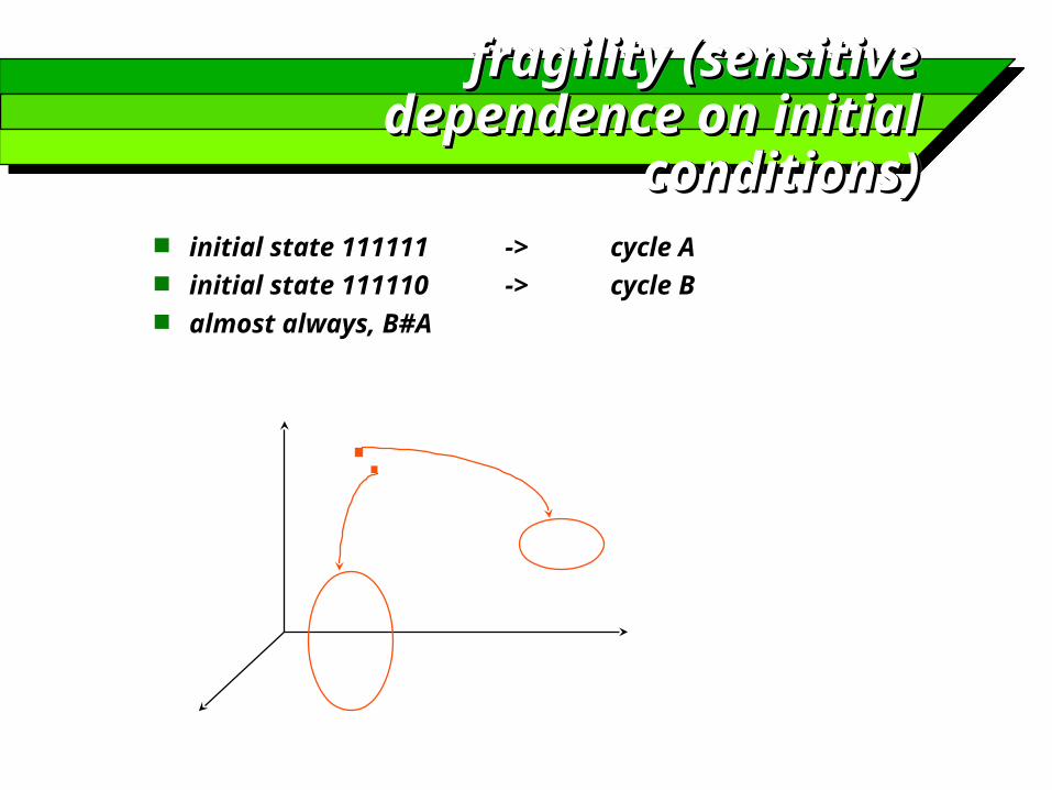
there are relatively few cycles wrt to the total number of states
cycles are long (their period grows as 2bN) systems are fragile with respect to small changes in
initial conditions nearby initial states go to different attractors the boundaries of the basins of attraction are highly irregular
analogous to “chaotic behaviour” in continuous dynamical systems
fragility (sensitive fragility (sensitive dependence on initial dependence on initial
conditions)conditions)
fragility (sensitive fragility (sensitive dependence on initial dependence on initial
conditions)conditions) initial state 111111 -> cycle A initial state 111110 -> cycle B almost always, B#A
low connectivitylow connectivitylow connectivitylow connectivity
if k= 2, cycle number scales as N1/2
cycle length grows as N1/2
basins are regular: systems starting from two nearby intial states usually evolve to the same attractor
the behaviour is much more regular and ordered than in the k=N-1 case
a phase transition accurs at some k value

regular basinsregular basinsregular basinsregular basins
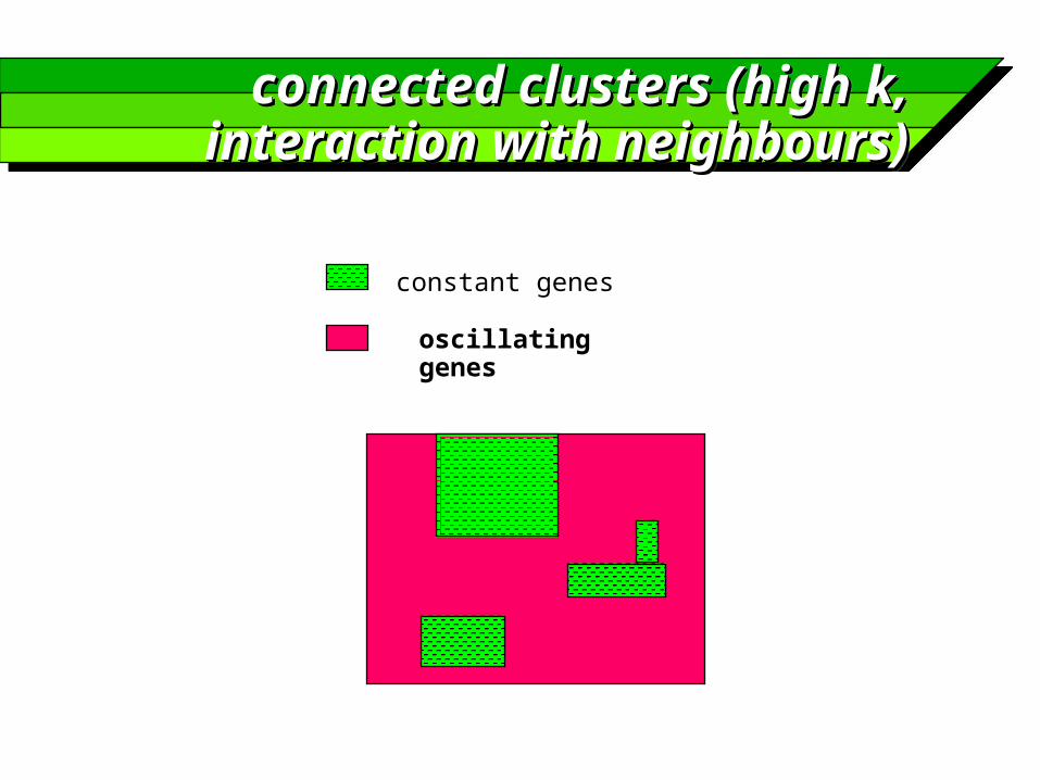
connected clusters (high k, connected clusters (high k, interaction with neighbours)interaction with neighbours)connected clusters (high k, connected clusters (high k,
interaction with neighbours)interaction with neighbours)
oscillating genes
constant genes

connected clusters (low k, connected clusters (low k, interaction with neighbours)interaction with neighbours)
connected clusters (low k, connected clusters (low k, interaction with neighbours)interaction with neighbours)
oscillating genes
constant genes

phase transitionphase transition
the network display a phase transition
by lowering the value of k, the transition takes place when the cluster of non oscillating genes percolates through the network
the boundary between ordered and disordered regimes can be found at different k values, if the set of boolean functions is restricted somehow
e.g. by limiting to canalyzing functions, i.e. those where at least one of the inputs has one values which forces the variable to take a specific value

order for freeorder for freeorder for freeorder for free
scaling laws in the self-organized regime number of cycles ~Nb (1/2<b<1) length of cycles ~Nb
the model is consistent with experimental observations over many different phyla
number of cellular types <-> number of different cycles cell life <-> length of cycles
selection builds upon the network self-organizing properties
the selective advantages of “the edge of chaos”?

warningwarning
the Kauffman model is a highly idealized representation of real genetic / metabolic nets which is based upon several approximations
no chemicals
proteins are fast wrt to the time step
synchronous activation may introduce “spurious cycles” in boolean dynamical systems (cfr. Hopfield nets)
fully random topology, constant k

butbut
the Kauffman model allows us to address issues which would otherwise be missed, and to develop an appropriate language in which we can frame some key questions
the very existence of self-organizing dynamics in nonlinear genetic networks
the importance of attractors in determining the properties of gene nets robustness and basins of attraction the importance of the average degree of connectivity
it also allows us to examine in a new way the interplay between selection and self-organization
the importance of studying ensembles of networks to gain information about their generic properties
continuous or booleancontinuous or boolean
the intermediate values of gene expression may be due to
intermediate values of the concentration of stimulating factors
time-dependent phenomena (transients, cycles)
the boolean approximation allows one to better elucidate the logic of control, but must be exercised with care
the boolean dynamics may be different from the continuous one
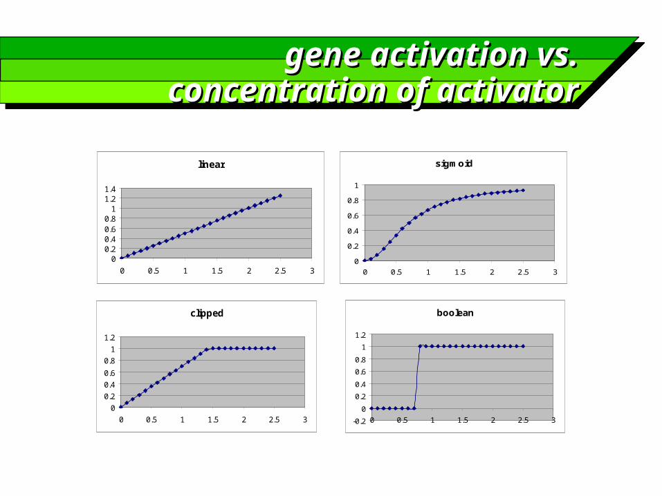
gene activation vs. gene activation vs. concentration of activatorconcentration of activator
linear
00.20.40.60.8
11.21.4
0 0.5 1 1.5 2 2.5 3
sigmoid
0
0.2
0.4
0.6
0.8
1
0 0.5 1 1.5 2 2.5 3
clipped
0
0.2
0.4
0.6
0.8
1
1.2
0 0.5 1 1.5 2 2.5 3
boolean
-0.2
0
0.2
0.4
0.6
0.8
1
1.2
0 0.5 1 1.5 2 2.5 3
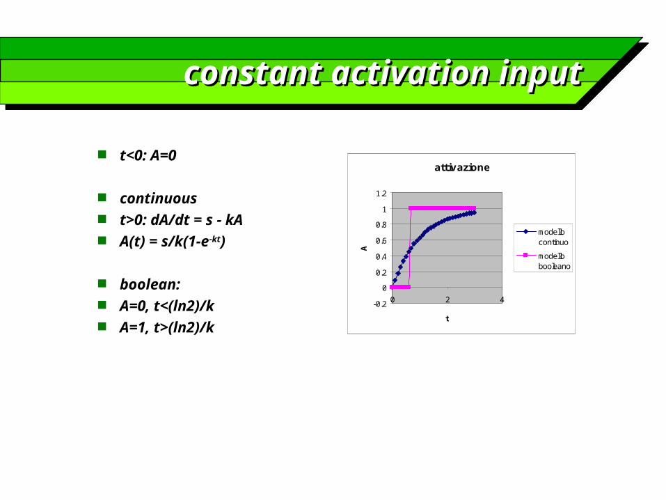
constant activation inputconstant activation input
t<0: A=0
continuous t>0: dA/dt = s - kA A(t) = s/k(1-e-kt)
boolean: A=0, t<(ln2)/k A=1, t>(ln2)/k
attivazione
-0.2
0
0.2
0.4
0.6
0.8
1
1.2
0 2 4
t
A
modellocontinuo
modellobooleano

generalizing Kauffmangeneralizing Kauffman
it would then be desirable to have a model where activations can take continuous values the “logic of control” is explicit and flexible as in Kauffman
there is an embarras de richesse in model development
we require that the models are true generalizations of the Kauffman RBN
they lead to the same dynamics if the initial activations are boolean
continuous model (Serra & continuous model (Serra & Villani)Villani)
let t be larger than the time required for protein synthesis and degradation (as in Kauffman)
ai = activation of gene i (normalized to [0,1]) i.e. concentration of the corresponding product
a = [a1, a2 .. aN] ai(t+1) = [contri(a(t))] where x: (x) 0 x 0: (x) = 0 x>0, >0: (x+) (x) for simplicity: limx->+ (x) = 1
for the time being, chemicals are not explicitly considered, as in Kauffman
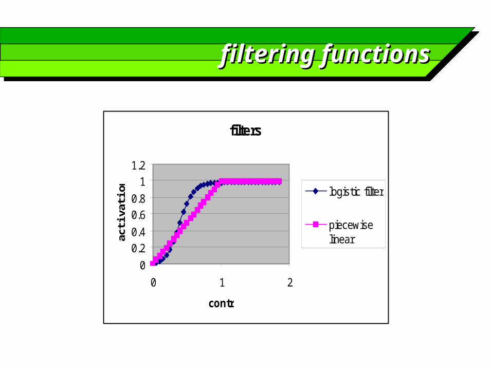
filtering functionsfiltering functions
filters
0
0.20.4
0.60.8
11.2
0 1 2
contr
activ
atio
n
logistic filter
piecewiselinear
summing over the pathssumming over the paths
let us focus upon the interactions among genes mediated of course by their synthesis products
i.e. consider ai(t+1) = (contri(a(t))
the “digital logic” of the genetic switch must be translated into a continuous rule
the transition rule for the activation must take into account contributions from all the combinations of [0,1] values of its inputs
for example, if the rule is an OR, it may receive positive contributions from the combinations of input values (11), (10), (01) (which tend to turn it on) and negative from (00) (which tends to turn it off
evolution lawsevolution lawsevolution lawsevolution laws
a “set of input values” (input set) to gene i, Yi = {yi1, y12} is defined as a given combination of boolean values of its input genes (in our case, 11, 10, 01 or 00)
generalization to K inputs is trivial
the truth table assigns a boolean function (the activation of the gene at the next time step) to each input set
we must define a weight for each input set, and a rule to combine the weights of the different input sets
Q1i set of the input paths to gene “i” which correspond to an updated value “1”
Q0i set of the input paths to gene “i” which correspond to an updated value “0”
weighting an input set weighting an input set (model A)(model A)
weighting an input set weighting an input set (model A)(model A)
the weight should be computed from the activations of the two input genes, i.e. from a1 and a2
the contribution of the input set (11) may be estimated to be limited by the gene with the smallest activation
(11) = min(a1, a2) the contribution of the input set (00) may be estimated
to be limited by the gene with the highest activation (00) = max(a1,a2) = min(1-a1, 1-a2) the contribution of (10) and (01) are (10) = min(a1, 1-a2) (01) = min(1-a1, a2)
the equations of model Athe equations of model Athe equations of model Athe equations of model A
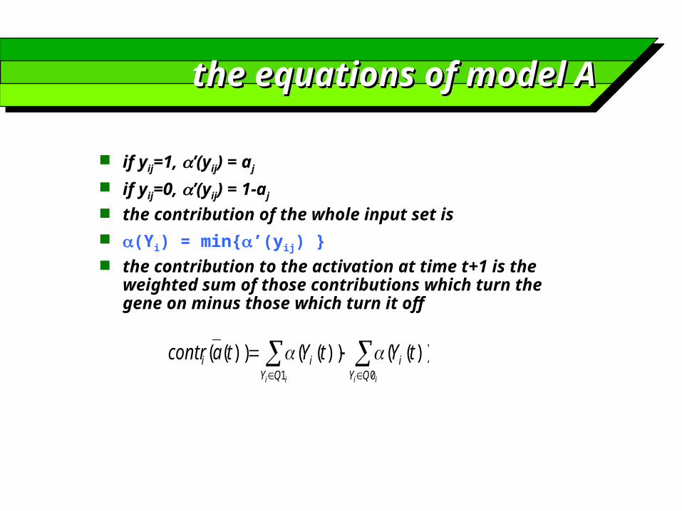
if yij=1, ’(yij) = aj
if yij=0, ’(yij) = 1-aj
the contribution of the whole input set is (Yi) = min{’(yij) } the contribution to the activation at time t+1 is the
weighted sum of those contributions which turn the gene on minus those which turn it off
iiii QY
iQY
ii tYtYtacontr01
))(())(())((
dynamical propertiesdynamical propertiesdynamical propertiesdynamical properties
let us start from a set of initial activations which belong all to {0,1}
for every gene, there is one input set which has contribution = 1, precisely the one which corresponds to the “right” 0’s and 1’s
all the other input sets provide a vanishing contribution (as there is at least one “1” corresponding to a “0” real value, or a “0” corresponding to a 1, which give ’(yij)=0
if the output corresponding to the only nonvanishing contribution is 1, then the next state is 1, otherwise it is 0
therefore the system always remains on the corners of the unit hypercube
and the rule for determining ai(t+1) is the same as that of the original Kauffman model
the model therefore represents a true generalization of the Kauffman model
towards the corners of the towards the corners of the unit hypercubeunit hypercube
it can be observed that starting from a set of intermediate values the system tends to reach the corners of the hypercube
at least in systems with few inputs per node if the sigma function is piecewise linear, it exactly reaches the corners if it is a logistic, it approaches the corners (provided that (1) 1)
it then behaves much like the Kauffman boolean model the reason can be understood by observing that
in some nodes there is an imbalance between the numbers of input pathways which turn the gene on or off
these systems tend to reach their extreme values and to drive also the remaining genes to boolean extremes
the dynamics is therefore similar to that of random boolean networks
model Bmodel Bmodel Bmodel B
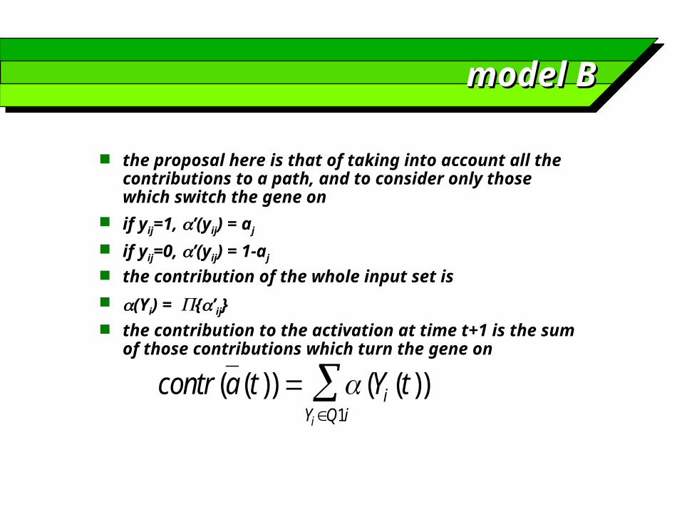
the proposal here is that of taking into account all the contributions to a path, and to consider only those which switch the gene on
if yij=1, ’(yij) = aj
if yij=0, ’(yij) = 1-aj
the contribution of the whole input set is (Yi) ={’ij} the contribution to the activation at time t+1 is the sum
of those contributions which turn the gene on
contr a t Y tiY Q ii
( ( )) ( ( ))
1

the features of model Bthe features of model B
model B would describe the properties of an ensemble of Kauffman (i.e. boolean) cells which
all have the same topology and the same boolean functions fro each node
evolve independently from each other starting from different initial conditions
if the different activations were independent which is not the case, due to the non ergodic evolution
of the system starting from a set of initial activations which belong all
to {0,1}, the system always remains on the corners of the unit hypercube, and the rule for determining ai(t+1) is the same as that of the Kauffman model
the model therefore represents a true generalization of the Kauffman model

the behaviour of model Bthe behaviour of model Bthe behaviour of model Bthe behaviour of model B
starting from random initial conditions the system can approach the corners of the unit hypercube evolve towards fixed points with nodes taking
intermediate values evolve towards cycles with nodes taking intermediate
values which usually have also a non oscillating part
therefore the continuous dynamics may differ from that of the original Kauffman model
yet features of self-organization are evident also in this case:
few attractors per network short cycle length
model improvementmodel improvement
different kinds of model, either boolean or continuous, display features of dynamical self-organization
it is important to explicitly take into account also the action of chemicals
morevoer, in order to describe processes as e.g. biodegradation of organic compounds, tumor growth, etc., it is necessary to take into account the process of cell proliferation
still in search of the generic properties number and characteristics of attractors scaling with network size influence of key parameters robustness of results vs. model changes (and not only vs. parameter
changes)
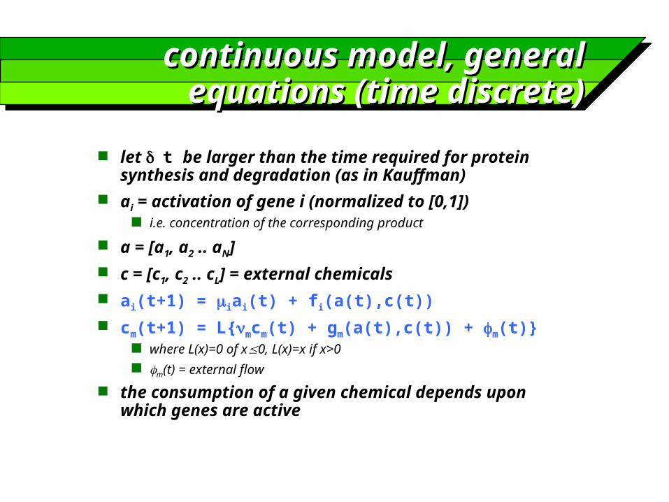
continuous model, general continuous model, general equations (time discrete)equations (time discrete)
let t be larger than the time required for protein synthesis and degradation (as in Kauffman)
ai = activation of gene i (normalized to [0,1]) i.e. concentration of the corresponding product
a = [a1, a2 .. aN] c = [c1, c2 .. cL] = external chemicals ai(t+1) = iai(t) + fi(a(t),c(t)) cm(t+1) = L{mcm(t) + gm(a(t),c(t)) + m(t)}
where L(x)=0 of x0, L(x)=x if x>0 m(t) = external flow
the consumption of a given chemical depends upon which genes are active

connectionsconnectionsconnectionsconnections
the equation for a(t) ai(t+1) = iai(t) + fi(a(t),c(t)) if dt is “long” i=0 the activation depends upon the chemicals as well as
upon the activation of other genes fi(a(t),c(t)) = [contri(a(t)) + i(a(t),c(t))] where x: (x) 0 x 0: (x) = 0 x>0, >0: (x+) (x) for simplicity: limx->+ (x) = 1 contri(a(t)) depends upon the activation of the other
genes

exampleexample
a constitutive gene is constantly expressed (activation a); there are N cells in a chemostat with constant flow rate
c(t+1) = L{c(t) - WaN + in + c} Pseudomonas stutzeri which degrades o-xylene
two operons, one for X->F->K, the other for F->K both controlled by the same promoter, activated by phenol both always expressed at a limited extent ignore differences in synthesis speed within a single operon
aT(t+1) = aT0+T(uTFcF) aP(t+1) = aP0+T(uPFcF) cX(t+1) = L{cX(t) - WXTN(t)aT(t)cX(t) + in -cX(t)} cF(t+1) = L{cF(t) + WFXN(t)aT(t)cX(t) - WFTN(t)aT(t)cF(t) -
WFPN(t)aP(t)cF(t) -cF(t)} + equations for N(t)
““energy”energy”““energy”energy”
to describe cell proliferation, only some genes are explicitly considered (the “green region”), while the effects of the cell’s standard genes (the “grey region”) are collectively described by a single variable
“energy” (i.e. excess resources) rules the reproduction rate, that is the cutoff on the activation values
energy decreases if there are no chemicals, increases due to gene-chemical interactions
let be the average “energy” per cell cell number decreases if energy is below its
“maintenance value” maint = (1-)/ allows a steady population (in the no flow
case)
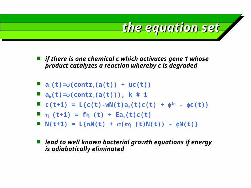
the equation setthe equation set
if there is one chemical c which activates gene 1 whose product catalyzes a reaction whereby c is degraded
a1(t)=(contr1(a(t)) + uc(t)) ak(t)=(contrk(a(t))), k # 1 c(t+1) = L{c(t)-wN(t)a1(t)c(t) + in - c(t)} (t+1) = f(t) + Ea1(t)c(t) N(t+1) = L{N(t) + ( (t)N(t)) - N(t)}
lead to well known bacterial growth equations if energy is adiabatically eliminated

simulationssimulationssimulationssimulations
C
-
Energy
++
+

the behaviour of model Athe behaviour of model Athe behaviour of model Athe behaviour of model A
the system tends to reach the corners of the unit hypercube
if u is such that the first gene is always active, N, c and tend to reach constant values;
activations oscillate as in the Kauffman model if u is smaller, oscillations in c, N and are observed the cycles are slightly longer than in Kauffman original
work different attractors are observed in these networks
an example (chemostat)an example (chemostat)an example (chemostat)an example (chemostat)
network Bc1 (random boolean laws) has three attractors a fixed point (N=170, A=15), with a basin of attraction
which covers 3% of the initial conditions tested a limit cycle (with N=constant, A cycles with period 4)
with a very small basin a limit cycle where N and A oscillate with period 16
(317<N<318, 9<A<17), which attracts 96% of the initial conditions - all the nodes oscillate

conclusionsconclusions
continuous activation values chemicals the growth of cell population
therefore allowing to model bacterial degradeation of organic compounds, tumor growth, etc.
continuous model provides results which are, the case of model A, very similar to those of the Kauffman model
as far as the gene-gene interactions are concerned
also different models display features of dynamical self-organization
the model allows to consider a more complicated set of interactions, preserving self-organization features similar to those of Kauffman

the topology of real networksthe topology of real networks
in our search for generic properties of genetic/metabolic networks we have so far assumed random connections
more precisely, in Kauffman models the number of connections per node, k, is fixed, the wiring is random with uniform probability distribution
an obvious generalization is that of allowing that also k may differ in different nodes
the theoretical model which better describes this topology is the random graph

random graphs (Erdos-random graphs (Erdos-Renyi)Renyi)
N labelled nodes undirected links the probability pij that node i and node j are connected
is equal for all (i,j)
pij=p binomial distribution of the number of links per node if p<<1, this gives rise to an approximate Poisson
probability distibution for the number of connections per node, k
p(k) = qke-q/k! with <k>=q=pN, sk= q = (pN)
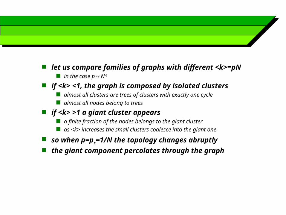
let us compare families of graphs with different <k>=pN in the case p N-1
if <k> <1, the graph is composed by isolated clusters almost all clusters are trees of clusters with exactly one cycle almost all nodes belong to trees
if <k> >1 a giant cluster appears a finite fraction of the nodes belongs to the giant cluster as <k> increases the small clusters coalesce into the giant one
so when p=pc=1/N the topology changes abruptly the giant component percolates through the graph

path lengthpath length
path length = 1
path length = 2
path length = 3
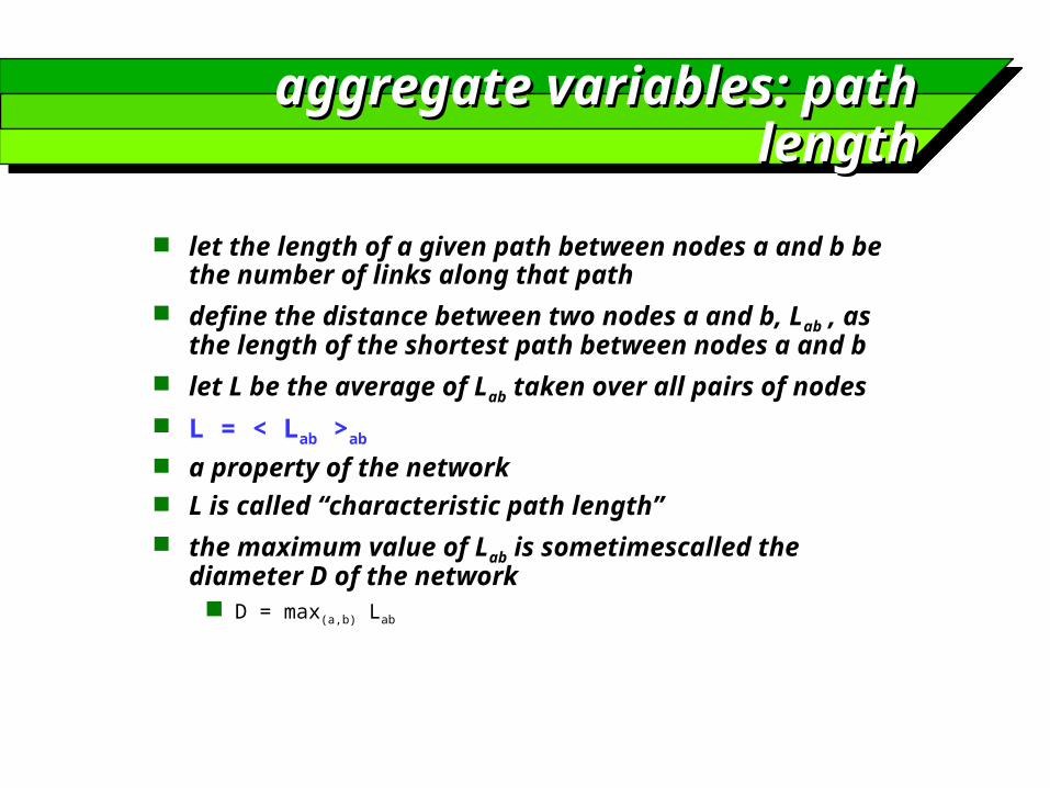
aggregate variables: path aggregate variables: path lengthlength
let the length of a given path between nodes a and b be the number of links along that path
define the distance between two nodes a and b, Lab , as the length of the shortest path between nodes a and b
let L be the average of Lab taken over all pairs of nodes L = < Lab >ab
a property of the network L is called “characteristic path length” the maximum value of Lab is sometimescalled the
diameter D of the network D = max(a,b) Lab
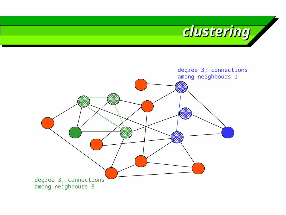
clusteringclustering
degree 3; connectionsamong neighbours 1
degree 3; connectionsamong neighbours 3

aggregate variables: aggregate variables: clustering coefficientclustering coefficient
consider first a given node, v, with kv connections let n(v) be the number of links which exist between the
nodes which are directly connected to node v the maximum number of links is nmax(v)= kv(kv-1)/2 let C(v) = n(v)/nmax(v)
C(v) is the clustering coefficient of node v it measures how likely it is that the neighbours of v are also connected
let C be the average of C(v) C = <C(v)>v
C is called the clustering coefficient of the graph it measures the average connectedness of the graph
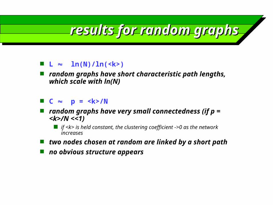
results for random graphsresults for random graphs
L ln(N)/ln(<k>) random graphs have short characteristic path lengths,
which scale with ln(N)
C p = <k>/N random graphs have very small connectedness (if p =
<k>/N <<1) if <k> is held constant, the clustering coefficient ->0 as the network
increases
two nodes chosen at random are linked by a short path no obvious structure appears

comparison with regular comparison with regular latticeslattices
consider a regular ring with connections to the K neighrest neighbours
the characteristic path length grows linearly with N L N/2K
for a D-dimensional regular lattice, L N1/D
the clustering coefficient is C=3(K-2)/[4(K-1)] C -> 3/4 in the limit of large K two nodes chosen at random are connected by a long
path the regular structure induces a high clustering

strange properties of real strange properties of real networks : small worldsnetworks : small worlds
many real networks display the small world phenomenon, i.e. they
are sparse: k<<N the number of connections per node is much smaller than the number of
nodes
have high clustering C >> Crandom
have short characteristic path length L Lrandom
so they combine high clustering with short paths neither random nor regular

models of small world models of small world networks: Watts & Strogatznetworks: Watts & Strogatz
start from a regular graph e.g. a ring with connections to k neirest neighbours
each link is rewired with probability p (one node is held fixed, the other is changed)
double links between the same two vertices are forbidden
if p->0 then L N/2k , C 3/4
long pathways, high clustering
for a broad range of nonzero p values L(p) << L(0), C(p) C(0) >> Crandom
short paths, high clustering
if p->1, random graph L lnN/lnk , C k/N

WS modelWS model
the WS model interpolates between regular and random graphs
the degree distribution p(k) is similar to the Poisson distribution of a random graph
almost all nodes have similar connectedness
the WS model shows that the introduction of some long range interactions (“shortcuts”) allows the shortening of the characteristic path lengths
so the small world phenomenon can take place in exponentially distributed networks - where all the nodes have a similar degree - with some long range connections
strange properties of real strange properties of real networks: scale-freedomnetworks: scale-freedom
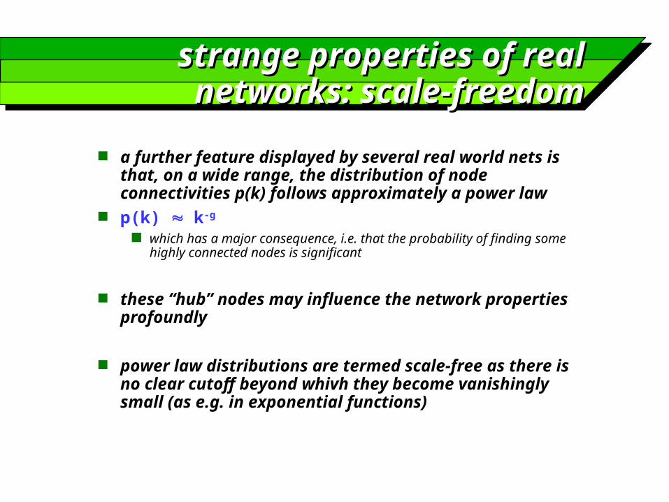
a further feature displayed by several real world nets is that, on a wide range, the distribution of node connectivities p(k) follows approximately a power law
p(k) k-g
which has a major consequence, i.e. that the probability of finding some highly connected nodes is significant
these “hub” nodes may influence the network properties profoundly
power law distributions are termed scale-free as there is no clear cutoff beyond whivh they become vanishingly small (as e.g. in exponential functions)
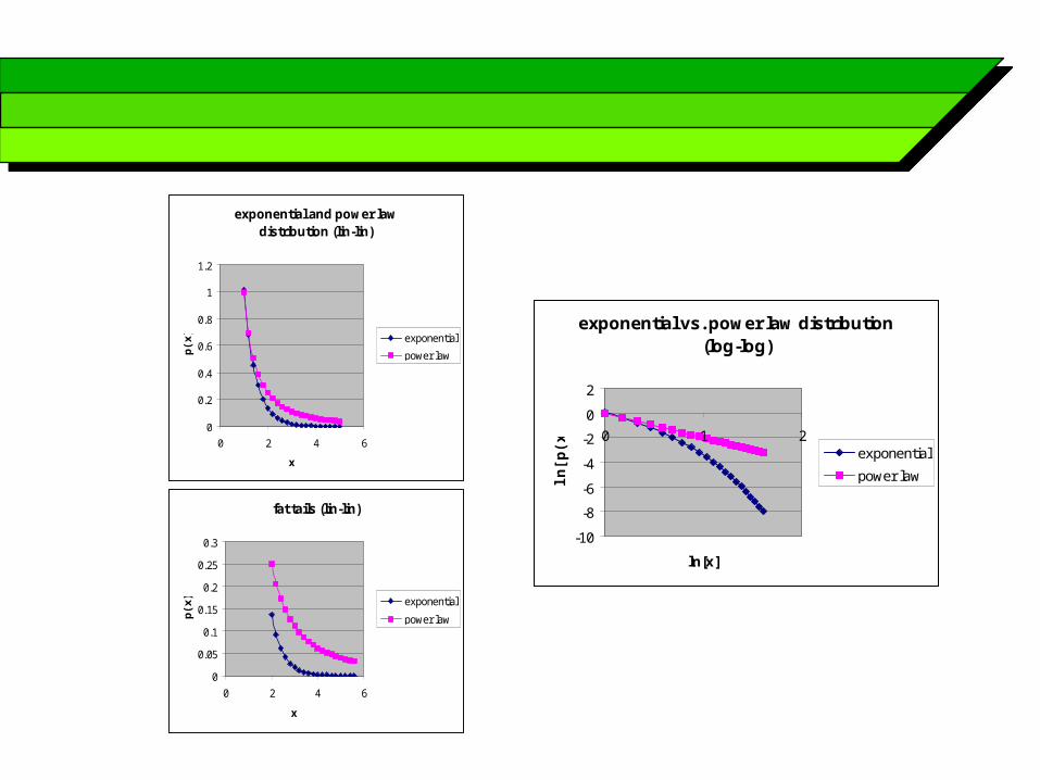
exponential and power law distribution (lin-lin)
0
0.2
0.4
0.6
0.8
1
1.2
0 2 4 6
x
p(x
) exponential
power law
fat tails (lin-lin)
0
0.05
0.1
0.15
0.2
0.25
0.3
0 2 4 6
x
p(x
) exponential
power law
exponential vs. power law distribution (log-log)
-10
-8
-6
-4
-2
0
2
0 1 2
ln[x]ln
[p(x
)] exponential
power law
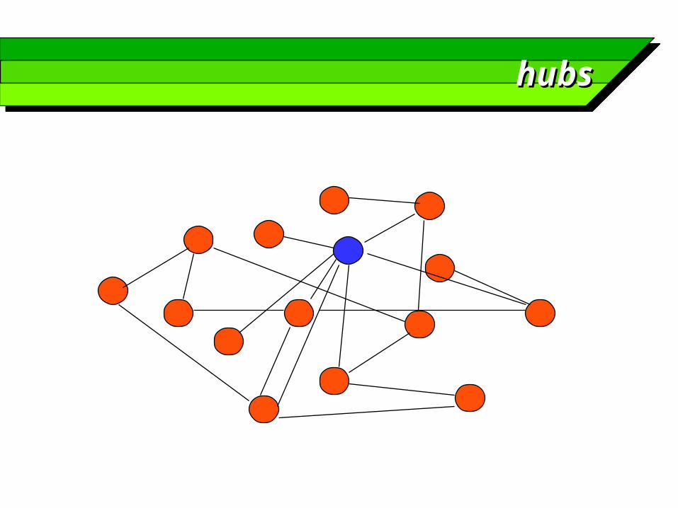
hubshubs

how do networks come into how do networks come into existence ?existence ?
random graphs and WS are both based on a fixed number of nodes and on drawing or rewiring connections
many real networks grow in time by addition of new nodes and links: Internet, genetic nets, telephone communications, etc.
moreover, in RG and WS the probability that a link is drawn to a node is independent from the number of existing links
in growing networks the probability that a new node is connected to an existing one may depend upon the connectivity of the latter (e.g. webpages, citations)
connectivity is a proxy for “importance”

models of scale-free models of scale-free networks: Barabasinetworks: Barabasi
start with a limited number m0 of nodes
at each step t add a new node and introduce m ( m0) edges which link the new node to m existing nodes
the probability that the new node is connected to the existing node i depends upon ki(t),
(ki) = ki/(j kj)
after T steps the network is composed by N=T+m0 T nodes and mT edges
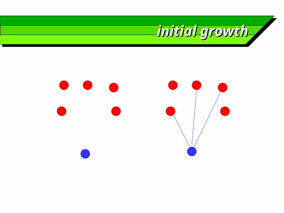
initial growthinitial growth

preferential attachmentpreferential attachment
properties of scale-free netsproperties of scale-free nets
simulations show that the probability distribution is scale free:
p(k) k-g, (g 3 independent of m) L lnN
short characteristic path length
the clustering coefficient is higher than in the random graph case, as the process introduces correlations among the node’s degrees
the clustering coefficient descreases as N increases, in contrast to WS
the SF networks display a different kind of small world phenomenon, their properties are influenced by the presence of a few hub nodes with a high degree
models and realitymodels and reality
Watts-Strogatz and scale-free networks are two theoretical small-world models which can be useful to interpret real networks of the “small world” type
the property derives either from shortcuts in WS from hubs in SF
real world networks may present either behaviour deciding which model better approximates a specific network is a matter
of empirical testing

metabolic network of metabolic network of escherichia coliescherichia coli
Wagner and Fell: aerobic growth on a minimal medium with glucose as sole carbon source
reactions concerning central routes of energy metabolism and synthesis of small molecules
glycolisis, pentose phosphate pathway, glycogen metabolism, TCA cycle, oxydative phosphorylation, amino acid and polyammine biosynthesis, nucleotide and nucleoside biosynthesis, glycerol 3-phosphate and membrane lipids, riboflavin, Co-A, NADP and others
287 substrates, 317 reactions substrate graph: nodes represent substrates, and there
is a link between two nodes if there is a reaction to which both substrates participate
Jeong et al: metabolic network analysis of 43 organisms (6 archea, 35 bacteria, 5 eucaryotes)
biological implicationsbiological implications
short diameters means that information about a “perturbation” (i.e. removal of a substrate or of a reaction) can rapidly propagate through the network
some properties of scale free networks are highly robust; for example, random removal of substrates does not appreciably alter the characteristic path length
however, scale free networks are vulnerable to removal of hubs