Embed Size (px)
Citation preview

Introduction to Generative Models
Piyush Rai
Machine Learning (CS771A)
Sept 23, 2016
Machine Learning (CS771A) Introduction to Generative Models 1

Generative Model
Defines a probabilistic way that could have “generated” the data
Each observation xn is assumed to be associated with a latent variable zn (we can think of zn as acompact/compressed “encoding” of xn)
zn is assumed to be a random variable with some prior distribution p(z |φ)
Assume another data distribution p(x |z , θ) that can “generate” x given z
What x and z “look like”, and the form of the distributions p(z |φ), p(x |z , θ) will beproblem-specific (we will soon look at some examples)
{θ, φ} are the unknown model parameters
The goal will be to learn {θ, φ} and zn’s, given the observed data
Machine Learning (CS771A) Introduction to Generative Models 2

“Generative Story” of Data
Generative models can be described using a “generative story” for the data
The “generative story” of each observation xn, ∀n
First draw a random latent variable zn ∼ p(z |φ) from the prior on z
Given zn, now generate xn as xn ∼ p(x |θ, zn) from the data distribution
Such models usually have two types of variables: “local” and “global”
Each zn is a “local” variable (specific to the data point xn)
(φ, θ) are global variables (shared by all the data points)
We may be interested in learning the global vars, or local vars, or both
Usually it’s possible to infer the global vars from local vars (or vice-versa)
Machine Learning (CS771A) Introduction to Generative Models 3

Why Generative Models?
A proper, probabilistic way to think about the data generation process
Allows modeling different types of data (real, binary, count, etc.) by changing the data distributionp(x |θ, z) appropriately
Can synthesize or “hallucinate” new data using an already learned model
Generate a “random” z from p(z |φ) and generate x from p(x |θ, z)
Allows handling missing data (by treating missing data also as latent variable)Hallucinated faces pic courtesy: http://torch.ch/blog/2015/11/13/gan.html
Machine Learning (CS771A) Introduction to Generative Models 4

Some “Canonical” Generative Models
Mixture model (used in clustering and probability density estimation)
Latent factor model (used in dimensionality reduction)
Can even combine these (e.g., mixture of latent factor models)
Machine Learning (CS771A) Introduction to Generative Models 5

Some “Canonical” Generative Models
Mixture model (used in clustering and probability density estimation)
Latent factor model (used in dimensionality reduction)
Can even combine these (e.g., mixture of latent factor models)
Machine Learning (CS771A) Introduction to Generative Models 5
Some “Canonical” Generative Models
Mixture model (used in clustering and probability density estimation)
Latent factor model (used in dimensionality reduction)
Can even combine these (e.g., mixture of latent factor models)
Machine Learning (CS771A) Introduction to Generative Models 5

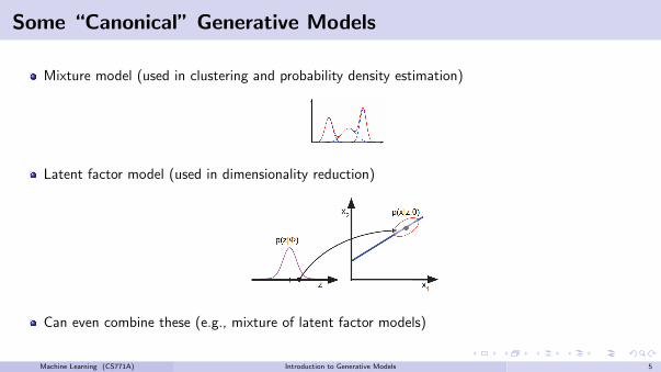
Example: Mixture Model
Assume data {xn}Nn=1 was generated from a mixture of K distributions
Suppose these K distributions are p(x |θ1), . . . , p(x |θK )
Don’t know which of the K distributions each xn was generated from
Consider the following generative story for each xn, n = 1, 2, . . . ,N
First choose a mixture component zn ∈ {1, 2, . . . ,K} as zn ∼ p(z |φ)
Now generate xn from the mixture component no. zn as xn ∼ p(x |θzn )
In a mixture model, z is discrete so p(z |φ) is a multinomial distribution
The data distribution p(x |θzn) depends on the type of data being modeled
Mixture models can model complex distributions as superposition of simpler distributions (can beused for density estimation, as well as clustering).
Machine Learning (CS771A) Introduction to Generative Models 6

Example: Latent Factor Model
Assume each D-dim xn generated from a K -dim latent factor zn (K � D)
Consider the following generative story for each xn, n = 1, 2, . . . ,N
First generate zn from a K -dim distr. as zn ∼ p(z |φ)
Now generate xn from a D-dim distr. as xn ∼ p(x |zn, θ)
When p(z |φ) and p(x |zn, θ) are Gaussian distributions, this basic generative model is called factoranalysis or probabilistic PCA
The choice of p(z |φ) and p(x |zn, θ) in general will be problem dependent
Many recent advances in generative models (e.g., deep generative models, generative adversarialnetworks, etc) are based on these basic principles
Machine Learning (CS771A) Introduction to Generative Models 7

Going Forward..
We will look at, in more detail, some specific generative models
Gaussian mixture model (for clustering and density estimation)
Factor Analysis and Probabilistic PCA (for dimensionality reduction)
We will also look at how to do parameter estimation in such models
One common approach is to perform MLE/MAP
However, presence of latent variables z makes MLE/MAP hard
Reason: Since z is a random variable, we must sum over all possible values of z when doingMLE/MAP for the model parameters θ, φ
log p(x |θ, φ) = log∑
z
p(x |z , θ)p(z |φ) (Log can’t go inside the summation!)
Expectation Maximization (EM) algorithm gives a way to solve the problem
Basic idea in EM: Instead of summing over all possibilities of z , make a “guess” z̃ and maximizelog p(x , z̃ |θ, φ) w.r.t. θ, φ to learn θ, φ. Use these values of θ, φ to refine your guess z̃ and repeat untilconvergence.
Machine Learning (CS771A) Introduction to Generative Models 8

Gaussian Mixture Model (GMM)
Assume the data is generated from a mixture of K Gaussians
Each Gaussian represents a “cluster” in the data
The distribution p(x) will be a weighted a mixture of K Gaussians
p(x) =∑
z
p(x, z) =∑
z
p(z)p(x|z) =K∑
k=1
p(z = k)p(x, z = k) =K∑
k=1
πkN (x|µk ,Σk )
where πk ’s are the mixing weights:∑K
k=1 πk = 1, πk ≥ 0 (intuitively, πk = p(z = k) is thefraction of data generated by the k-th distribution)
The goal is to learn the params {µk ,Σk}Kk=1 of these K Gaussians, the mixing weights {πk}Kk=1,and/or the cluster assignment zn of each xn
GMM in many ways improves over K -means clustering
Machine Learning (CS771A) Introduction to Generative Models 9

GMM Clustering: Pictorially
Some synthetically generated data (top-left) generated from a mixture of 3 overlapping Gaussians(top-right).
Notice the “mixed” colored points in the overlapping regions in the final clusteringMachine Learning (CS771A) Introduction to Generative Models 10

Next Class
GMM in more detail. Extensions of GMM.
Parameter estimation in GMM
The Expectation Maximization (EM) algorithm
Machine Learning (CS771A) Introduction to Generative Models 11