Introduction to Functional Programming with SML to Functional Programming with SML Dr. Cong-Cong Xing Dept of Mathematics and Computer Science . ... If there are any issues that need

Introduction to Functional

Programming with SML

Dr. Cong-Cong Xing

Dept of Mathematics and

Computer Science

Before We Start

Course website:

http://math.nicholls.edu/xing

Everything regarding the course

should/can be found on this site.

Any questions? Contact me.

• If there are any issues that need more

explanations, I’ll provide separate detailed

Word/PDF documents for them.



Chapter 1

A Few Words About Functional

Programming

Special Note

• This “Chapter 1” is not exactly the chapter 1 in

the textbook. I compiled the materials myself.

• Please go through the materials and

understand them as best as you can. We will

come back revisiting some of them when we

know some basics of ML programming; and in

that case/time, you will understand the

material better. (Of course, if you want to

understand everything completely at this

point, you are welcome to try to do so…)

The World of Programming

Paradigms

mainstream

programming,

“easy” to write, but

hard to prove

(maintain)

imperative functional

logical

programming

Becoming

increasingly popular,

theoretically

founded, strong

math flavor,

elegant.

A totally different

story

obj-oriented

What is Functional Programming

(FP)?

We will try to understand FP via

comparison w/ traditional imperative

programming.

Examples of imperative programming

languages: C, C++, Pascal, Java (and

more…. your own examples? what about Python? Is

Python functional?)

Python stuff…

ML stuff ...

compare it w/

the Python

screen ....

what can you

see in terms

of difference?

More about

this later on ...

Imperative programming base: von Neumann

architecture computer

Functional programming base: math functions

Which one is superior?

• No winner/loser.

Pure functional programming has no side

effects

Imperative programming “depends on” side

effects

Side-effect Example (in terms of

objects)

x=1 a.x<=2

Obj a

x=1 a.x<=2 x=2

Obj a Obj b Functional

Obj a

x=2

Override data field x of a Obj a

Imperative

x=1

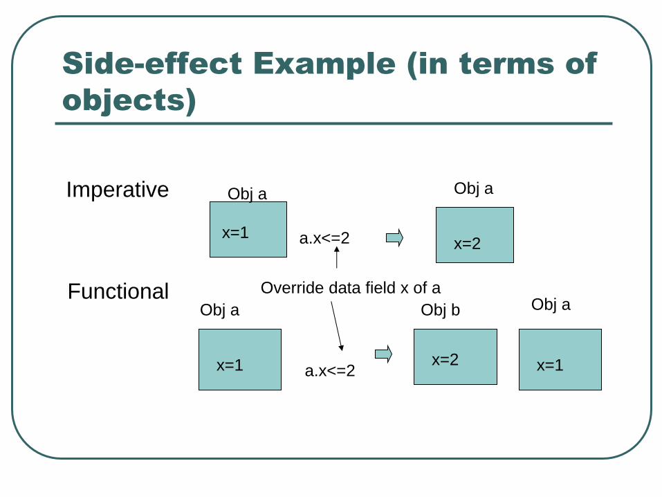
Functions (our old friend)

(normal) math notation: f(x) =x+1

Lambda-notation: λx.x+1 (will talk about it later on)

Math notation gives a name to a function whereas lambda notation does not.

Higher-order functions: functions that take a function as argument and/or returns a function as the result. (how to do this in Java?)

• Higher-order function ex: the function-

composition function ˚ : (it takes 2 functions

and produces another function)

g ˚ f

( or we name it as fcomp(f, g) if we want)

Questions: how can we do this w/ imperative

programming?

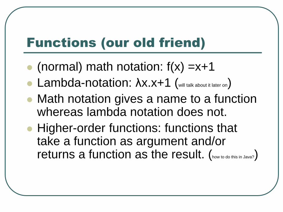
(most important) Features of

Imperative Programming

“Fine” processing. Computation consists of many individual movements and computations of small items of data

Programming by side-effect. Computation proceeds by continually changing the “state” of the machine – the values stored in memory locations – by assignments.

Iteration is the predominant control structure. Functions, esp. recursive functions, take a back seat.

The language structures, both data and

control, are fairly close to the underlying

(real) computer (hardware) architecture.

• Ex: goto --- unconditional jump

array --- consecutive blocks of memory

pointer --- memory location address

assignment --- data movement

variable --- memory cell/location

(most important) Features of

Functional Programming

All computations are carried out by

function applications

For pure functional programming

• No side effects

• No need for variables (in the sense of

imperative programming) and assignment

statements

Cannot be replaced by the functions in

imperative languages (why not?)

Question to think about ...

Given a function in math

f(x) = x + k for some 𝑘 ∈ 𝑅

What is difference between x and k?

Is k a variable?

Can k have difference values?

Is k a constant?

what about x?

Chapter 2

Getting Started with ML

0. Standard ML New Jersey

(SML/NJ)

• We will be using a particular implementation

of ML: SML/NJ in this class.

• SML/NJ is freely available at www.smlnj.org/.

• Once installed, a successful invocation of

SML/NJ should give you something like this

http://www.smlnj.org/




• Please read Chapter 1 of the textbook (for

details). It should be straightforward to read

as there is no programming yet in this

chapter.

• The major points in this chapter are

summarized here.

1. How to invoke ML?

Typically, the following two ways to

invoke the system should be sufficient

• Type sml at command prompt to get an

interactive mode

• C:\sml (for Windows)

• % sml (for Unix)

• To run a file (program) w/ the system:

• C:\sml < filename (Windows)

• % sml < filename (Unix)

2. How to terminate ML?

Type the following at command line

• ^z (ctrl z, Windows)

• ^d (ctrl d, Unix)

• (Note (for math grad students): do not worry

about Unix if you are not familiar w/ it. In case

you are wondering what Unix is, think of

Mac…)

3. Expressions

• This is important: in a sense, everything

(every program you type) in ML is an

expression.

• Every expression is going to be evaluated (or

computed).

• There are simple expressions and complex

expressions. Complex expressions are

evaluated to become simpler expressions

which are further evaluated to become values.

• In a sense, this is somehow like evaluating (or

computing) a mathematical expression…

• ex: evaluate (a + b)/2 where a, b are

variables and hold some values.

• Think about this: when the expression (a+b)/2

gets evaluated in math, what will happen?

Will the evaluation of (a+b)/2 cause any other

unintentional changes (side effect??)

1. A preliminary ex:

Expression 1+2

is typed/entered

“val” stands for

value “it” represents the

expression just evaluated

by the system

Or, 3 is bound to variable it.

The result of

evaluating the

expression 1+2

The type of the

result of the

evaluation

2. Ground (or primitive) types

• Integers (int)

• Same as other languages. Note: “~”, not “-”, is

used to denote the negative sign in ML. Ex: 23,

45, ~12.

• Reals (real)

• Same as other languages. Ex: 0.123, 4.52, ~1.2,

2.0, 2e10 (2 × 1010 )

• Booleans (bool)

• true, false

• Strings (string)

• sequence of symbols included within “”.

• Ex: “abc”, “a”, “x723y-”, “”.

• Characters (char)

• A single character. Ex: #”a”, #”8”. (Note the

symbol #. It is not part of the character, but a way

to signify that what follows is a character.)

• Q: since ‘a’ is not used to represent character in

ML, what would ‘a’ in ML represent (think about it

and try to answer it later on)?

3. Arithmetic operations

Symbol Operation precedence

~ Unary minus/negative High

* Multiplication

/ Real division

div Integer division

mod Modulo

+ Addition (not a positive sign)

- Subtraction (not a negative sign) Low same

same

• Ex: Expression value

~3 + 4 1

4~3 ?

+4+1 ?

4+3.0 ?

4*3.0 ?

4.0 mod 1.0 ?

4 mod 2 0

2/4 ?

2 div 4 0

2.0/4.0 0.5

? means to figure

out the answer by

yourself. You can

try them out easily

using the

interactive mode of

the system.

4. String concatenation

• s^w = sw (put strings s and w together)

• Ex: “progra”^ “mming” = “programming”

5. Relational operators

• Almost the same as other languages.

• Summarized in the following table. • Note: = is not assignment operator, it is a comparison

operator. What would be the ML’s response for a = 4

(suppose variable a is defined already)?

ML Math meaning

= Equal

<> Not equal

< Less than

<= Less than or equal

> Greater than

>= Greater than or equal

Note: ML does not allow reals to be compared by = or <>. This

may be different from other languages, but makes a good point

in the sense that no machines/hardware can really tell whether

two real numbers are equal in every case.

• Ex:

Ex:

This shows: = is the

comparison

operator, not

“assignment”

Then, what about the “=“ in value

binding, say, val a = 1; ? Is that “=“

“assignment”?

6. Logical operators

Ex:

ML Logical meaning

not logical NOT

andalso logical AND

orelse logical OR (inclusive)

7. Conditional expression

• if E then F else G ⇒ 𝐹 𝑖𝑓 𝐸 = 𝑡𝑟𝑢𝑒𝐺 𝑖𝑓 𝐸 = 𝑓𝑎𝑙𝑠𝑒

* here, ⇒ should be understood as “evaluates

to”. E, F, and G are sub-expressions.

* if_then_else_ is an operator, taking 3

arguments

• Ex:

if (1=1) then 2 else 3 evaluates to 2

if (1<2) then 3 else 2.0 = ?

(try it yourself. Hint: this is an expression, and

therefore must have a type. Every expression in ML

must have a type, and (almost) everything in ML is

an expression. See special note on next slide)

• Note: if E then F else G in ML is an

(evaluable) expression, just like 3+4 is an

expression. This is different from the if-then-

else construct found in other languages such

as C and Java, and is actually one of the

fundamental differences between them.

Students used to imperative programming w/

these languages need to pay special attention

to this point.

Can you think of an example that shows

the fundamental difference between if-

then-else in ML and Java, in the sense

that it is an expression in ML (and not so

in Java)? (left as a hw)

4. Type Consistency

• ML is strongly typed. Some operators are

overloaded (e.g. +), some are not (e.g. /).

Either way, operands of different types cannot

be taken by a binary operator.

• Ex:

expression legal?

1+2.0 No (why?)

1+2 Yes

1.0+2.0 Yes

Expression Legal?

1.0/2 No (why?)

1.0/2.0 Yes

1/2 No (why?)

Coercion between different types

coercion Function meaning example

From int to

real

real convert to

real

real 1 = 1.0

from real to

int

floor,

ceil,

round,

trunc

floor

ceiling

round

truncate

round 3.5=4

round ~3.5 = ~4

floor 2.3 = 2

floor ~2.3=~3

ceil 2.3 =3

ceil ~2.3 =~2

trunc 2.3 =2

trunc ~2.3=~2

coercion function meaning example

from character to

ASCII

ord returns argument’s

ASCII code

ord #”A” = 65

from int to

character

chr reversal of ord chr 65 = #”A”

chr 66 = #”B”

chr (ord #”a”)=#”a”

5. Variables and Environments

1. Identifiers

• Alphanumeric identifiers

{A-Z,a-z,’} {A-Z,a-z,’,0-9,_}*

(for a set A, A* is the set of all (finite) strings formed by

elements in A)

One

element

from this

set

Followed by one

element (a string)

from this set

ex: A, a, a1, yr1,

ex: ‘a, ‘b (they are type variables)

• Symbolic identifier

Strings drawn from

+ - * / < > = ! @ # $ % ^ & …(see p 28 in text)

Ex: +++, $=, << (looks strange?)

but

be mindful about spaces

in this case.

ok w/o space

not ok w/o space

Note:

• Symbolic ids are mainly used to operators.

• Don’t mix symbolic ids w/ alphanumeric ids.

• My personal advice: avoid using symbolic ids.

but may be useful

sometime. E.g., does it

look nice? Simulation of

the ++ in Java?

2. Environment • An environment consists of identifier bindings.

When ML is invoked, the default environment is

given, where all meaningful ids are bound to their

values. Environment changes during

computations by adding new entries of bindings,

and can be generally viewed as something similar

to a stack. (what is a stack?)

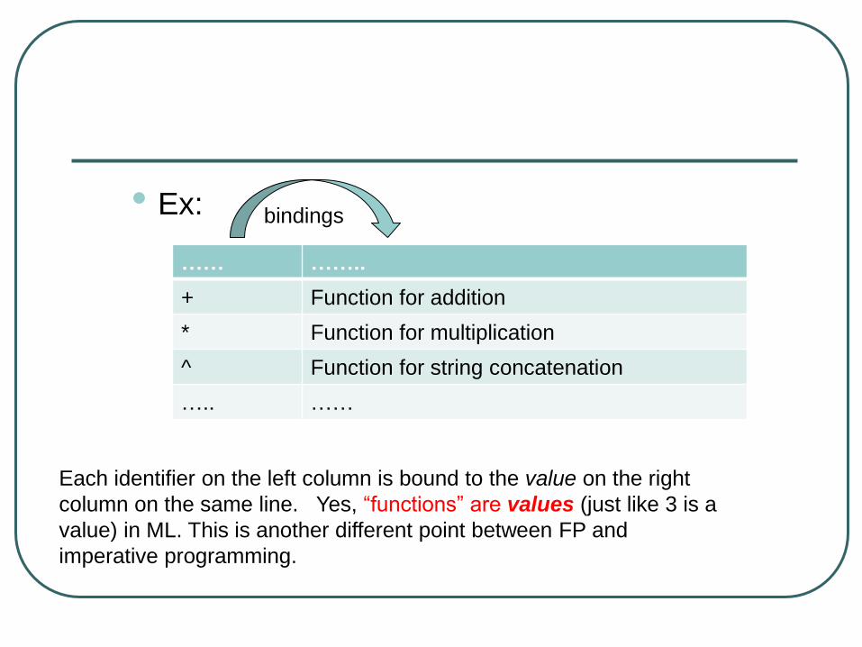
• Ex:

…… ……..

+ Function for addition

* Function for multiplication

^ Function for string concatenation

….. ……

bindings

Each identifier on the left column is bound to the value on the right

column on the same line. Yes, “functions” are values (just like 3 is a

value) in ML. This is another different point between FP and

imperative programming.

3. How to bind identifiers to values? Syntax: val <id> = <expression>

Ex: val a = 1;

val b = 2;

val c = a+b;

id value

c 3

b 2

a 1

…. …

result in

environment

• Note: val-declaration/definition is NOT the

assignment statement in imperative

programming languages (such as C and

Java). Rather, they are fundamentally

different. (What is the exact difference?) This is related

to the side-effect issue that was mentioned in

chapter 1 of this note.

6. Basic data structures: tuples

and lists

1. Tuples

the same notion tuples 𝑎1, … , 𝑎𝑛 as in math.

syntax: (exp1, exp2, … , exp𝑖) 𝑖 ≥ 2

type: 𝑇1∗ 𝑇2 ∗ ⋯∗ 𝑇𝑖

ex: (1,2) : int*int

(1, 2, 3.1) : int*int*real

(1,2, (1,2)) : int*int*(int*int)

(the product of sets in

math)

what if i=1?

• note: one way to understand tuple (e1,e2)

with type T1*T2 is that (e1,e2) is an element

of the set T1 x T2 (Cartesian product) (if we

regard a type as a set). For this reason, types

like T1*…*Ti are also called product type.

• note: 𝑖𝑛𝑡 ∗ 𝑖𝑛𝑡 ∗ 𝑖𝑛𝑡 ≠ 𝑖𝑛𝑡 ∗ 𝑖𝑛𝑡 ∗ 𝑖𝑛𝑡

≠ 𝑖𝑛𝑡 ∗ 𝑖𝑛𝑡 ∗ 𝑖𝑛𝑡

in particular,

ML evaluates

(1, 2, 3) = (3, 4, 5)

to the false value

in particular,

ML does not evaluate

(1,1,1) = ((1,1),1)

to false. It refuses to evaluate it, which means the two

sides are not even comparable.

2. Get components of tuples • syntax: #<i> <tuple>

• ex:

3. Lists • syntax: [exp1, exp2, … , exp𝑖] 𝑖 ≥ 0,

all expressions must be of the same type.

• type: T list where T is the type of the elements in

the list

• ex:

[1,2,3] : int list

[1]: int list

[] : ‘a list (why ‘a - type variable- here?)

[“a”, “ab”] : string list

• note:

• type is a central issue in ML.

• we start seeing two type constructors now –

product type constructor and list type constructor –

which allow us to build complex types from simple

ones.

• remember the slogan: everything in ML must have

a type. Type, typed, typing.

more on the type constructors

• __ list is the list type constructor; it takes a

type and returns another type

• what is the product type constructor? * or

*_*_..._*?

4. Operations on lists • Destructive operations.

• DEF: for a list [𝑙1, 𝑙2, … , 𝑙𝑛], the head of the list is 𝑙1

, and the tail of the list is [𝑙2, … , 𝑙𝑛].

• In ML, the head and tail of a list are given by the

built-in operators hd and tl.

• ex:

Q:Isn’t the type of

[] ‘a list? why int

list here?

• constructive operation

• :: (called cons traditionally) which works the

opposite way to head and tail operators. It takes

as arguments an element 𝑎 and a list [𝑙1, … , 𝑙𝑛], and returns [𝑎, 𝑙1, … , 𝑙𝑛].

[𝑎, 𝑙1, … , 𝑙𝑛]

[𝑙1, … , 𝑙𝑛] 𝑎

𝑐𝑜𝑛𝑠 ℎ𝑑 𝑡𝑙

what is the idea

behind all these

operation?

induction or

recursion !

types of these primitive list operators

• ex:

1:: 2 :: 3 :: [] (explanation of the last one)

= 1 :: (2 :: (3 :: [])) ( :: is right-associative)

= 1 :: (2 :: [3])

= 1 :: [2,3]

= [1,2,3] : int list

can’t be left-associative:

((1::2)::3)::[]

• @: ‘a list * ‘a list ‘a list

it takes two list of the same type and returns the

concatenation of the two list. (disjoint union)

• ex:

5. Three functions

• implode: char list string

it takes a list of chars and return the string

made of those chars in the given order

• ex:

• explode: string char list

it is the opposite of implode.

• ex:

• concat: string list string

it takes a list of strings and concatenates the strings

in the list into one (long) string.

• ex:

Not to be confused w/ list concatenation @.

6. Type constructions in ML • (Basis) int, real, bool, char, string are ground

types.

• we can inductively define more types using the

ground types:

• (Induction) if T1, T2, …, Tn are types, then so is

T1*T2*…*Tn (type for tuples).

• if T is a type, then so is T list (type for list).

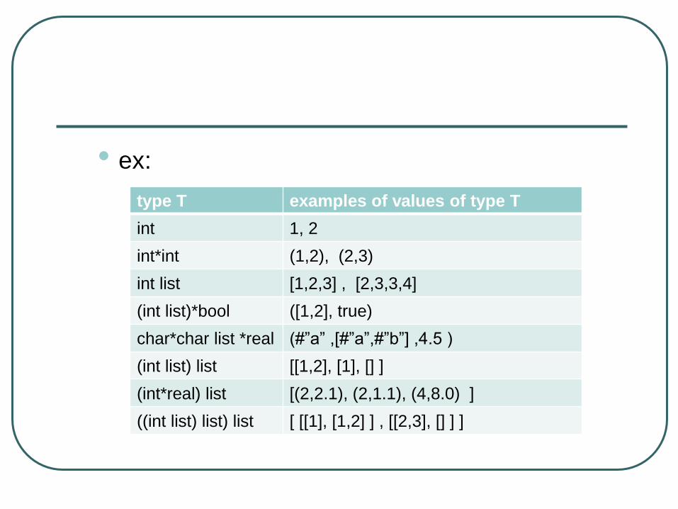
• ex:

type T examples of values of type T

int 1, 2

int*int (1,2), (2,3)

int list [1,2,3] , [2,3,3,4]

(int list)*bool ([1,2], true)

char*char list *real (#”a” ,[#”a”,#”b”] ,4.5 )

(int list) list [[1,2], [1], [] ]

(int*real) list [(2,2.1), (2,1.1), (4,8.0) ]

((int list) list) list [ [[1], [1,2] ] , [[2,3], [] ] ]

Summary of concatenations

• We have encountered 3 concatenations. Do

not confuse them.

function meaning example

^ string concatenation “ab”^”cd” =“abcd”

@ list concatenation [1,2]@[3,4] =

[1,2,3,4]

concat concatenate strings in a

list into a (new) string

concat [“ab”, “cd”]

= “abcd”

Chapter 3 Defining Functions

1. Overview -- How to define

functions?

There are at least 3 ways to define

functions in ML.

• “fun” way:

• Ex: fun f(x) = x+1;

• “value-binding” way:

• Ex: val f = fn x => x+1;

• “𝜆-way” (anonymous way)

• Ex: fn x => x+1; (𝜆𝑥. 𝑥 + 1)

• The “fun” way is what we are familiar with, and is

consistent w/ usual math notations. It is also

widely used in other programming languages. We

will primarily focus on this way (in this section).

• The “value-binding” way emphasizes the fact that

in FP paradigm a function is nothing but a value

(just like 3 is a value) that can be bound to an

identifier. (3 can be bound to an identifier too, of

course)

• The first 2 ways all give a name to a function when

defining that function. But, a function does not

need a name to exist. (or does it? What is exactly a

function anyway?) The lambda way to define

functions illustrates this point; it is a direct

rephrase of the 𝜆-abstraction in 𝜆-calculus (which is

an alternative direct study on functions).

prominent appearance of the

symbol lambda

1. How to define functions?

• Syntax: fun <id> (list of para) = <exp>

• ex:

• Write a function that converts a lowercase letter to

an upper-case one.

fun upper c = chr (ord c -32)

note: you don’t need to

specify the type of

parameters in function

definition; ML will do its

best to detect its type

(when it can).

• ex: write a ML function that implements

𝑓 𝑥 = 𝑥2 for real numbers x.

• fun sq(x:real) = x*x;

Q: why need

the “real”

after x?

What if it is

not there?

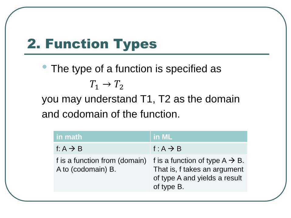
2. Function Types

• The type of a function is specified as

𝑇1 → 𝑇2

you may understand T1, T2 as the domain

and codomain of the function.

in math in ML

f: A B f : A B

f is a function from (domain)

A to (codomain) B.

f is a function of type A B.

That is, f takes an argument

of type A and yields a result

of type B.

Question: OK, do we see a new type

constructor here? If yes, how do we

describe it mathematically (i.e. regard it

as a function w/ domain and codomain)

Answer: ???

ex:

ex: the following are all function types.

int int

(real * real) int

int (int int) (what is this?)

(Is the writing int -> int -> int potentially confusing?)

int list int

‘a ‘a (what is this?)

the type of sq is

real real. That is,

sq: R R in math.

• note: “” is right-associative (in ML). That is,

ML stipulates that

𝑇1 → 𝑇2 → 𝑇3 ≡ 𝑇1 → (𝑇2→ 𝑇3)

for any types 𝑇1, 𝑇2, 𝑎𝑛𝑑 𝑇3.

Q: how ML denote the type Type equation here. (𝑇1→ 𝑇2) → 𝑇3 then?

3. Type annotations

• ML will try its best to deduce the type of

everything (by its well-known type inference

algorithm). But, when what given by ML is not

what you want, you may have to specify the

types explicitly.

• ex: no type

annotation for x

Since you didn’t

tell ML the type of

x, ML infers type

int -> int for sq

by itself.

• ex:

• ex:

This time, x is clearly

specified to be of type

real. So ML recognizes

it.

This is an identify

function on integers, i.e.,

id takes an integer and

returns that integer

immediately. (note the

type of id is int -> int

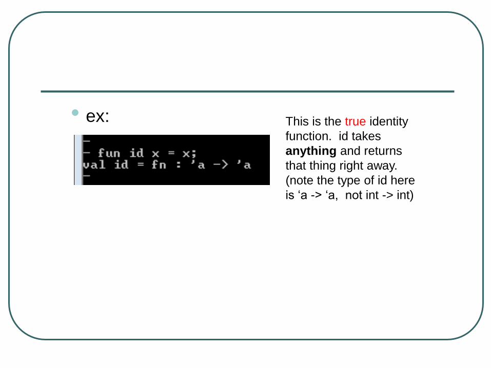
• ex: This is the true identity

function. id takes

anything and returns

that thing right away.

(note the type of id here

is ‘a -> ‘a, not int -> int)

4. Comments

• (* ….. *)

• Anything in between (* and *) will be ignored

by ML compiler.

• Comments are used for the purposed of

documentation.

5. Functions w/ more than one

parameters

A

B

C C A x B ≅

Conceptually, in math, functions that take

TWO arguments (one from set A and one

from set B) can be regarded as a function that

takes ONE argument from the set AxB.

Ex: a function that takes two arguments

f(x,y) = x + y

can be isomorphically regarded as a function that take

one argument (an order pair)

f ((x,y)) = (x,y)1 + (x,y)2

(where (x,y)i means the i-th component of the pair)

Why don’t we just write f ((x,y)) = x + y? (left as a hw)

• In ML, the fact that functions taking two

arguments are regarded as functions taking

one argument can be seen from the types.

Note this is the type of one element –-

a 2-tuple (pair)

This verifies that f takes one

argument (a 2-tuple)

• Ex: find the largest among 3 integers.

Note: this is literally just

one argument, not 3

arguments

6. External Variables in Function

Definitions

• When a function is defined, the reference to

external variables (variables not defined in the

body of the function) is determined by the

current environment at the defining time, and

will not be affected by subsequent changes to

the environment.

• Ex:

x is external to f, and x=3

when f is defined

x has now a new binding

f 2 is 5 not 12, which shows the

x used in f is still 3.

but x has value 10 (the

new value).

• Note that in imperative languages, this would

be a different situation. A piece of Java code

that does similar thing is given below (next

slide). C or Pascal would do the same thing

as Java does. (This would be an example

illustrating the difference between variable

binding in FP and variable assignment in

imperative programming)

Value of x used in f(2)

is 10, not 3.

(Remember, ML’s

response is 5)

Current value of x is 10

see also slides 7 – 8 for Python vs ML example

7. Recursive Functions

• Idea: recursion (or induction) in math. (You

might want to review the mechanism of

mathematical inductions….)

• There are two things you need to know about

recursion:

• Basis: this is where the recursion stops.

• Inductive step: the computation w/ “large”

arguments is reduced to computations w/ “smaller”

arguments. (one step backward toward basis)

7. Recursion vs. Induction

Recursion

• Basis: this is where the

recursion stops (ending

point)

• Recursive step: the

computation w/ “large”

arguments is reduced to

computations w/ “smaller”

arguments. (one step

backward toward basis)

Induction

• Basis: this is where the

induction starts (staring

point)

• Inductive step: the validity

of a property w/ “large”

value depends on the

validity w/ “smaller” value.

(one step forward)

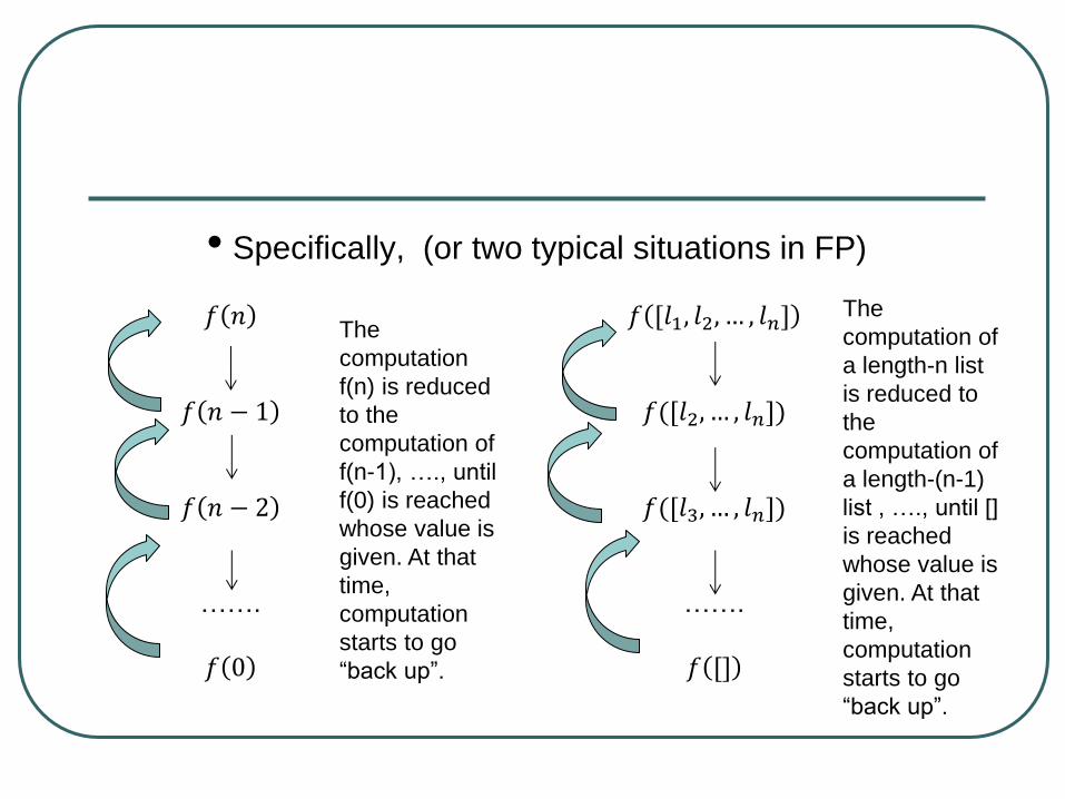
• Specifically, (or two typical situations in FP)

𝑓 𝑛

𝑓 𝑛 − 1

𝑓 𝑛 − 2

…….

𝑓 0

𝑓 [𝑙1, 𝑙2, … , 𝑙𝑛]

𝑓([𝑙2, … , 𝑙𝑛])

𝑓([𝑙3, … , 𝑙𝑛])

…….

𝑓 []

The

computation

f(n) is reduced

to the

computation of

f(n-1), …., until

f(0) is reached

whose value is

given. At that

time,

computation

starts to go

“back up”.

The

computation of

a length-n list

is reduced to

the

computation of

a length-(n-1)

list , …., until []

is reached

whose value is

given. At that

time,

computation

starts to go

“back up”.

• Ex: (classical ex) write a function f that reverses

any list. E.g.,

• f [1,2,3] => [3, 2, 1]

• f [“a”, “b”, “c”] => [“c”, “b”, “a”]

• analysis: the reversal of a length-n list can be

reduced to the reversal of a length-(n-1) list (see

the picture on the previous slide)

• basis: easy, the reversal of [] is just [] itself.

• inductive step: the reversal of the list 𝑙1, 𝑙2, … , 𝑙𝑛

can be computed as the reversal of 𝑙2, … , 𝑙𝑛

concatenated w/ 𝑙1

• ML code for f (just one line)

note the type of f. (the textbook has an error/typo

regarding this example: the type variable is ‘’a, not

‘a, in this case.

‘a means any type, ‘’a means those types whose

values can be compared by the = operator. Read

textbook for more details/explanations if you would

like.

Warning does

not mean the

code will not

work; instead, it

means the code

may have some

limitations. We

will learn a better

way of writing

the same

function later on.

execution of f on

different lists

But, does not work on real list (note: the

‘’Z list type)

• detailed exposition of the evaluation (or reduction)

of f [1,2,3]. (“=>” means evaluates; “->” means “is

bound to”) (Please read the following

computation carefully.)

• recursive call expansion is in red

• actual “build-up” (which occurs “on the way back”

of the recursive call) of list is in blue

f [1,2,3]

(if L=nil then nil else f(tl L) @ [hd L] | L -> [1,2,3])

f [1,2,3]


( f(tl L)@[hd L] | L -> [1,2,3])

f [1,2,3]


( f(tl L)@[hd L] | L -> [1,2,3])

f [2,3] @ ([hd L] | L -> [1,2,3])

f [1,2,3]


( f(tl L)@[hd L] | L -> [1,2,3])

f [2,3] @ ([hd L] | L -> [1,2,3])

(if L=nil then nil else f(tl L)@[hd L] | L -> [2,3])

@ ([hd L] | L -> [1,2,3])

f [1,2,3]


( f(tl L)@[hd L] | L -> [1,2,3])

f [2,3] @ ([hd L] | L -> [1,2,3])


@ ([hd L] | L -> [1,2,3])

( f(tl L) @ [hd L] | L -> [2,3] )

@ ([hd L] | L -> [1,2,3])

f [1,2,3]


( f(tl L)@[hd L] | L -> [1,2,3])

f [2,3] @ ([hd L] | L -> [1,2,3])


@ ([hd L] | L -> [1,2,3])

( f(tl L) @ [hd L] | L -> [2,3] )

@ ([hd L] | L -> [1,2,3])

(f [3] @ ([hd L] | L -> [2,3]) )

@ ([hd L] | L -> [1,2,3])

( (if L=nil then nil else f(tl L)@ [hd L] | L -> [3])

@ ([hd L] | L -> [2,3]) )

@ ([hd L] | L -> [1,2,3])

=> ( (f(tl L) @ [hd L] | L -> [3])

@ ([hd L] | L -> [2,3]) )

@ ([hd L] | L -> [1,2,3])

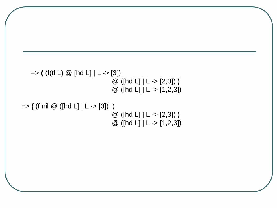
=> ( (f(tl L) @ [hd L] | L -> [3])

@ ([hd L] | L -> [2,3]) )

@ ([hd L] | L -> [1,2,3])

=> ( (f nil @ ([hd L] | L -> [3]) )

@ ([hd L] | L -> [2,3]) )

@ ([hd L] | L -> [1,2,3])

=> ( (f(tl L) @ [hd L] | L -> [3])

@ ([hd L] | L -> [2,3]) )

@ ([hd L] | L -> [1,2,3])

=> ( (f nil @ ([hd L] | L -> [3]) )

@ ([hd L] | L -> [2,3]) )

@ ([hd L] | L -> [1,2,3])

=> ( ( (if L=nil then nil else f(tl L)@[hd L] | L -> [])

@ ([hd L] | L -> [3]) )

@ ([hd L] | L -> [2,3]) )

@ ([hd L] | L -> [1,2,3])

stack

=> ( ( nil @ ([hd L] | L -> [3]) )

@ ([hd L] | L -> [2,3]) )

@ ([hd L] | L -> [1,2,3])

=> ( ( nil @ ([hd L] | L -> [3]) )

@ ([hd L] | L -> [2,3]) )

@ ([hd L] | L -> [1,2,3])

( ( nil @ [3] )

@ ([hd L] | L -> [2,3]) )

@ ([hd L] | L -> [1,2,3])

“pop up” the

stack

=> ( ( nil @ ([hd L] | L -> [3]) )

@ ([hd L] | L -> [2,3]) )

@ ([hd L] | L -> [1,2,3])

( ( nil @ [3] )

@ ([hd L] | L -> [2,3]) )

@ ([hd L] | L -> [1,2,3])

( [3] @ ([hd L] | L -> [2,3]) )

@ ([hd L] | L -> [1,2,3])

“pop up” the

stack

=> ( ( nil @ ([hd L] | L -> [3]) )

@ ([hd L] | L -> [2,3]) )

@ ([hd L] | L -> [1,2,3])

( ( nil @ [3] )

@ ([hd L] | L -> [2,3]) )

@ ([hd L] | L -> [1,2,3])

( [3] @ ([hd L] | L -> [2,3]) )

@ ([hd L] | L -> [1,2,3])

( [3] @ [2] ) @ ([hd L] | L -> [1,2,3])

“pop up” the

stack

=> ( ( nil @ ([hd L] | L -> [3]) )

@ ([hd L] | L -> [2,3]) )

@ ([hd L] | L -> [1,2,3])

( ( nil @ [3] )

@ ([hd L] | L -> [2,3]) )

@ ([hd L] | L -> [1,2,3])

( [3] @ ([hd L] | L -> [2,3]) )

@ ([hd L] | L -> [1,2,3])

( [3] @ [2] ) @ ([hd L] | L -> [1,2,3])

[3,2] @ ([hd L] | L -> [1,2,3])

“pop up” the

stack

=> ( ( nil @ ([hd L] | L -> [3]) )

@ ([hd L] | L -> [2,3]) )

@ ([hd L] | L -> [1,2,3])

( ( nil @ [3] )

@ ([hd L] | L -> [2,3]) )

@ ([hd L] | L -> [1,2,3])

( [3] @ ([hd L] | L -> [2,3]) )

@ ([hd L] | L -> [1,2,3])

( [3] @ [2] ) @ ([hd L] | L -> [1,2,3])

[3,2] @ ([hd L] | L -> [1,2,3])

[3,2] @ [1]

“pop up” the

stack

=> ( ( nil @ ([hd L] | L -> [3]) )

@ ([hd L] | L -> [2,3]) )

@ ([hd L] | L -> [1,2,3])

( ( nil @ [3] )

@ ([hd L] | L -> [2,3]) )

@ ([hd L] | L -> [1,2,3])

( [3] @ ([hd L] | L -> [2,3]) )

@ ([hd L] | L -> [1,2,3])

( [3] @ [2] ) @ ([hd L] | L -> [1,2,3])

[3,2] @ ([hd L] | L -> [1,2,3])

[3,2] @ [1]

[3,2,1]

(it takes a longongongongongong….. process to get the job done)

“pop up” the

stack

8. more recursion examples

• 𝑛𝑚

means the number of ways of choosing m

items out of n items.

• we know, from math, that

𝑛𝑚

= 𝑛−1𝑚

+ 𝑛−1𝑚−1

(can you prove it?)

Write a ML function that computes 𝑛𝑚

with n ≥ m.

4

2

32

31

22

21

21

20

11

10

11

10

Above: ML code.

Right: recursive calls of

c(4,2). Recursions stop

at each leaf and return

values “backward” the

tree.

4

2

32

31

22

21

21

20

11

10

11

10

Above: ML code.

Right: order of calls

being returned

9

6 7 3 2

1

10

4

5

11

8

9. Mutual Recursion

• Idea:

• syntax:

f = …. g.....

g = ….f….

f is defined using g

g is defined using f

fun <def of f>

and <def of g>

(note: and is a keyword here.)

• Ex: write functions odd and even that work in the

following way:

• odd L = list of odd-numbered (old-positioned) items

of L

• even L = list of eve-numbered (even-positioned)

items of L

• e.g.

odd [1,2,3] = [1,3]

even [1,2,3,4] = [2,4]

odd [] = [], even [] = []

odd [1] = [1], even [1] =[]

x o x …………

- How to express odd (L) in terms of even on a shorter list

than L?

- “o” indicates odd positions; “x” indicates even positions

o o

hd L tl L

x o x …………


than L?

- odd L = hd L :: even (tl L)


o o

hd L tl L

x o x …………


than L?


- How to express even (L) in terms of odd on a shorter list

than L?


o o

hd L tl L

x o x …………


than L?


- How to express even (L) in terms of odd on a shorter list

than L?

- even L = odd (tl L)


o o

hd L tl L

code and

execution

10. Define Functions using

Patterns

• This is a feature of that you do not see in

imperative languages.

• a pattern is roughly a structure w/ variables.

• syntax:

• fun <id><pat1> = <exp2>

| <id><pat2> = <exp2>

| …………

| <id><patn> = <expn>;

(1) the “x::xs” pattern

• Since every non-empty list can be regarded as a

head “con-ed” with a tail, so the patter x::xs matches

any non-empty list with x being bound to the head

and xs being bound to the tail.

• ex: Revisit of the list-reversal function

note the type of rev1.

Here, we have ‘a list, not

‘’a list.

x::xs

pattern

works for real list

this is the list-reversal

code we had before.

Note the type is ‘’a list,

not ‘a list. This function

does not work for list of

reals.

“a – refers to “equality types”:

types whose values can be tested

for equality. E.g., int, bool, char

are equality types, real is not.

(2) pattern “as” well as non-pattern

• syntax: <id> as <pat>

• ex: r as x::xs

when r as x::xs matches a list L, r gets the value of L

(no pattern here), x gets the head of L, and xs gets

the tail of L (patter is used).

• Ex: write a function that merges two sorted int

lists into one. For instance,

• merge ([1,2], [3,4]) = [1,2,3,4]

• merge ([1,3,4], [2,6]) = [1,2,3,4,6]

analysis: given the two sorted lists L and M,

we can carry out the desired merge recursively.

x xs

L

y ys

M

merge(L,M) would involve

inductive step:

• if x<y, then x :: merge(xs, M)

• otherwise, y :: merge(L,ys)

basis step:

and the basis would be reached when either list

becomes empty list, and in that case, just return the

other list

(note: L and M must be already sorted before

submitted to merge function)

workout the two examples to “visualize” how the

merge program works

• merge ([1,2], [3,4]) = [1,2,3,4]

• merge ([1,3,4], [2,6]) = [1,2,3,4,6]

• (3) anonymous variables

In pattern, when we need a variable but its name is not

important (or does not matter), we can use underscore (_) in

place of this variable. Roughly, _ means “anything, but we don’t

care about its name”.

Ex: write a function that always returns 1 (no matter what kind of

input given to this function.)

note: _ is not essential in the sense

that we can just replace _ by a ‘normal’

variable (say, x) but do not use x in the

body of the function. _ is just another

convenient feature provided by ML.

note, again,

the power of

ML: f can

take any kind

of arguments

(yes, even a

function) and

produce 1.

This is hard

to achieve in

Pascal or

Java.

g is a function defined

earlier.

• (4) formal definition of patterns • see pp 358-359 in textbook

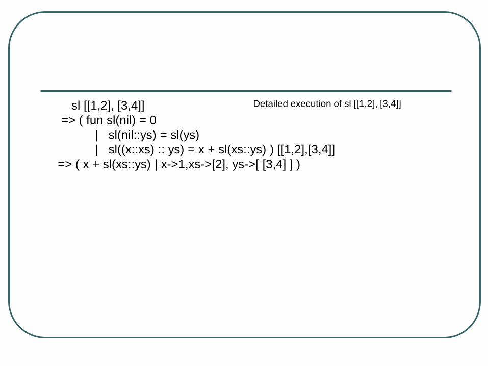
• (5) another example: What does this program sl do?

Let’s figure out its type first.

fun sl(nil) = 0

| sl(nil::ys) = sl(ys)

| sl((x::xs) :: ys) = x + sl(xs::ys);

how to deduce a type?

fun sl(nil) = 0


| sl((x::xs) :: ys) = x + sl(xs::ys);

this (nil) tells us that the

argument of sl is a list

this tells us that the

head of the arg list to sl

is also a list, from which

we (or ML) can deduce

that sl takes a list of

lists as argument.

this tells us that

the x is of type

int (default type

of + operator) since x is of type int, x::xs must

be an int list, and consequently

(x::xs)::ys must a (int list) list.

this tells us that sl

returns an integer.

Hence, sl has type:

int list list -> int

3

6

4

5

2

1

sl [[1,2], [3,4]]

Detailed execution of sl [[1,2], [3,4]]

sl [[1,2], [3,4]]

=> ( fun sl(nil) = 0


| sl((x::xs) :: ys) = x + sl(xs::ys) ) [[1,2],[3,4]]


sl [[1,2], [3,4]]



| sl((x::xs) :: ys) = x + sl(xs::ys) ) [[1,2],[3,4]]

=> ( x + sl(xs::ys) | x->1,xs->[2], ys->[ [3,4] ] )


sl [[1,2], [3,4]]



| sl((x::xs) :: ys) = x + sl(xs::ys) ) [[1,2],[3,4]]

=> ( x + sl(xs::ys) | x->1,xs->[2], ys->[ [3,4] ] )

1 + sl([2] :: [ [3,4] ])


sl [[1,2], [3,4]]



| sl((x::xs) :: ys) = x + sl(xs::ys) ) [[1,2],[3,4]]

=> ( x + sl(xs::ys) | x->1,xs->[2], ys->[ [3,4] ] )

1 + sl([2] :: [ [3,4] ])

1 + sl([ [2], [3,4] ])


sl [[1,2], [3,4]]



| sl((x::xs) :: ys) = x + sl(xs::ys) ) [[1,2],[3,4]]

=> ( x + sl(xs::ys) | x->1,xs->[2], ys->[ [3,4] ] )

1 + sl([2] :: [ [3,4] ])

1 + sl([ [2], [3,4] ])

=> 1 + ( fun sl(nil) = 0


| sl((x::xs) :: ys) = x + sl(xs::ys) ) [[2], [3,4]]


sl [[1,2], [3,4]]



| sl((x::xs) :: ys) = x + sl(xs::ys) ) [[1,2],[3,4]]

=> ( x + sl(xs::ys) | x->1,xs->[2], ys->[ [3,4] ] )

1 + sl([2] :: [ [3,4] ])

1 + sl([ [2], [3,4] ])

=> 1 + ( fun sl(nil) = 0


| sl((x::xs) :: ys) = x + sl(xs::ys) ) [[2], [3,4]]

1 + ( x + sl(xs::ys) | x->2, xs->[], ys->[ [3,4] ] )


sl [[1,2], [3,4]]



| sl((x::xs) :: ys) = x + sl(xs::ys) ) [[1,2],[3,4]]

=> ( x + sl(xs::ys) | x->1,xs->[2], ys->[ [3,4] ] )

1 + sl([2] :: [ [3,4] ])

1 + sl([ [2], [3,4] ])

=> 1 + ( fun sl(nil) = 0


| sl((x::xs) :: ys) = x + sl(xs::ys) ) [[2], [3,4]]

1 + ( x + sl(xs::ys) | x->2, xs->[], ys->[ [3,4] ] )

1 + 2 + sl([] :: [[3,4]])


sl [[1,2], [3,4]]



| sl((x::xs) :: ys) = x + sl(xs::ys) ) [[1,2],[3,4]]

=> ( x + sl(xs::ys) | x->1,xs->[2], ys->[ [3,4] ] )

1 + sl([2] :: [ [3,4] ])

1 + sl([ [2], [3,4] ])

=> 1 + ( fun sl(nil) = 0


| sl((x::xs) :: ys) = x + sl(xs::ys) ) [[2], [3,4]]

1 + ( x + sl(xs::ys) | x->2, xs->[], ys->[ [3,4] ] )

1 + 2 + sl([] :: [[3,4]])

1 + 2 + sl([ [], [3,4] ])


sl [[1,2], [3,4]]



| sl((x::xs) :: ys) = x + sl(xs::ys) ) [[1,2],[3,4]]

=> ( x + sl(xs::ys) | x->1,xs->[2], ys->[ [3,4] ] )

1 + sl([2] :: [ [3,4] ])

1 + sl([ [2], [3,4] ])

=> 1 + ( fun sl(nil) = 0


| sl((x::xs) :: ys) = x + sl(xs::ys) ) [[2], [3,4]]

1 + ( x + sl(xs::ys) | x->2, xs->[], ys->[ [3,4] ] )

1 + 2 + sl([] :: [[3,4]])

1 + 2 + sl([ [], [3,4] ])

=> 1 + 2 + ( fun sl(nil) = 0


| sl((x::xs) :: ys) = x + sl(xs::ys) ) [[], [3,4]]


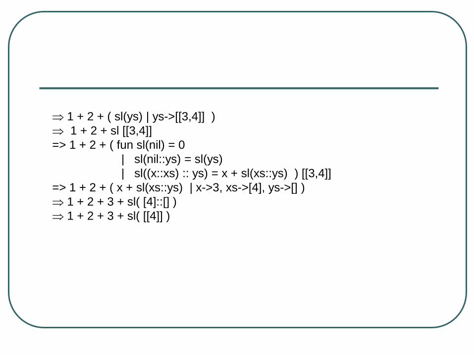
1 + 2 + ( sl(ys) | ys->[[3,4]] )

1 + 2 + ( sl(ys) | ys->[[3,4]] )

1 + 2 + sl [[3,4]]

1 + 2 + ( sl(ys) | ys->[[3,4]] )

1 + 2 + sl [[3,4]]

=> 1 + 2 + ( fun sl(nil) = 0


| sl((x::xs) :: ys) = x + sl(xs::ys) ) [[3,4]]

1 + 2 + ( sl(ys) | ys->[[3,4]] )

1 + 2 + sl [[3,4]]

=> 1 + 2 + ( fun sl(nil) = 0


| sl((x::xs) :: ys) = x + sl(xs::ys) ) [[3,4]]

=> 1 + 2 + ( x + sl(xs::ys) | x->3, xs->[4], ys->[] )

1 + 2 + ( sl(ys) | ys->[[3,4]] )

1 + 2 + sl [[3,4]]

=> 1 + 2 + ( fun sl(nil) = 0


| sl((x::xs) :: ys) = x + sl(xs::ys) ) [[3,4]]

=> 1 + 2 + ( x + sl(xs::ys) | x->3, xs->[4], ys->[] )

1 + 2 + 3 + sl( [4]::[] )

1 + 2 + ( sl(ys) | ys->[[3,4]] )

1 + 2 + sl [[3,4]]

=> 1 + 2 + ( fun sl(nil) = 0


| sl((x::xs) :: ys) = x + sl(xs::ys) ) [[3,4]]

=> 1 + 2 + ( x + sl(xs::ys) | x->3, xs->[4], ys->[] )

1 + 2 + 3 + sl( [4]::[] )

1 + 2 + 3 + sl( [[4]] )

1 + 2 + ( sl(ys) | ys->[[3,4]] )

1 + 2 + sl [[3,4]]

=> 1 + 2 + ( fun sl(nil) = 0


| sl((x::xs) :: ys) = x + sl(xs::ys) ) [[3,4]]

=> 1 + 2 + ( x + sl(xs::ys) | x->3, xs->[4], ys->[] )

1 + 2 + 3 + sl( [4]::[] )

1 + 2 + 3 + sl( [[4]] )

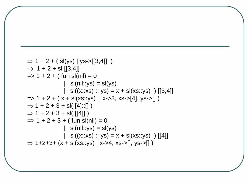
=> 1 + 2 + 3 + ( fun sl(nil) = 0


| sl((x::xs) :: ys) = x + sl(xs::ys) ) [[4]]

1 + 2 + ( sl(ys) | ys->[[3,4]] )

1 + 2 + sl [[3,4]]

=> 1 + 2 + ( fun sl(nil) = 0


| sl((x::xs) :: ys) = x + sl(xs::ys) ) [[3,4]]

=> 1 + 2 + ( x + sl(xs::ys) | x->3, xs->[4], ys->[] )

1 + 2 + 3 + sl( [4]::[] )

1 + 2 + 3 + sl( [[4]] )

=> 1 + 2 + 3 + ( fun sl(nil) = 0


| sl((x::xs) :: ys) = x + sl(xs::ys) ) [[4]]

1+2+3+ (x + sl(xs::ys) |x->4, xs->[], ys->[] )

1 + 2 + ( sl(ys) | ys->[[3,4]] )

1 + 2 + sl [[3,4]]

=> 1 + 2 + ( fun sl(nil) = 0


| sl((x::xs) :: ys) = x + sl(xs::ys) ) [[3,4]]

=> 1 + 2 + ( x + sl(xs::ys) | x->3, xs->[4], ys->[] )

1 + 2 + 3 + sl( [4]::[] )

1 + 2 + 3 + sl( [[4]] )

=> 1 + 2 + 3 + ( fun sl(nil) = 0


| sl((x::xs) :: ys) = x + sl(xs::ys) ) [[4]]

1+2+3+ (x + sl(xs::ys) |x->4, xs->[], ys->[] )

1+2+3+4 + sl([]::[])

1 + 2 + ( sl(ys) | ys->[[3,4]] )

1 + 2 + sl [[3,4]]

=> 1 + 2 + ( fun sl(nil) = 0


| sl((x::xs) :: ys) = x + sl(xs::ys) ) [[3,4]]

=> 1 + 2 + ( x + sl(xs::ys) | x->3, xs->[4], ys->[] )

1 + 2 + 3 + sl( [4]::[] )

1 + 2 + 3 + sl( [[4]] )

=> 1 + 2 + 3 + ( fun sl(nil) = 0


| sl((x::xs) :: ys) = x + sl(xs::ys) ) [[4]]

1+2+3+ (x + sl(xs::ys) |x->4, xs->[], ys->[] )

1+2+3+4 + sl([]::[])

1+2+3+4 +sl( [[]] )

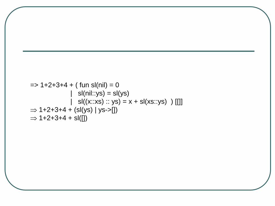
=> 1+2+3+4 + ( fun sl(nil) = 0


| sl((x::xs) :: ys) = x + sl(xs::ys) ) [[]]

=> 1+2+3+4 + ( fun sl(nil) = 0


| sl((x::xs) :: ys) = x + sl(xs::ys) ) [[]]

1+2+3+4 + (sl(ys) | ys->[])

=> 1+2+3+4 + ( fun sl(nil) = 0


| sl((x::xs) :: ys) = x + sl(xs::ys) ) [[]]

1+2+3+4 + (sl(ys) | ys->[])

1+2+3+4 + sl([])

=> 1+2+3+4 + ( fun sl(nil) = 0


| sl((x::xs) :: ys) = x + sl(xs::ys) ) [[]]

1+2+3+4 + (sl(ys) | ys->[])

1+2+3+4 + sl([])

=>1+2+3+4+ ( fun sl(nil) = 0


| sl((x::xs) :: ys) = x + sl(xs::ys) ) []

=> 1+2+3+4 + ( fun sl(nil) = 0


| sl((x::xs) :: ys) = x + sl(xs::ys) ) [[]]

1+2+3+4 + (sl(ys) | ys->[])

1+2+3+4 + sl([])

=>1+2+3+4+ ( fun sl(nil) = 0


| sl((x::xs) :: ys) = x + sl(xs::ys) ) []

1+2+3+4+0

=> 1+2+3+4 + ( fun sl(nil) = 0


| sl((x::xs) :: ys) = x + sl(xs::ys) ) [[]]

1+2+3+4 + (sl(ys) | ys->[])

1+2+3+4 + sl([])

=>1+2+3+4+ ( fun sl(nil) = 0


| sl((x::xs) :: ys) = x + sl(xs::ys) ) []

1+2+3+4+0

10

What we see with the system. (of course,

the system hides the details of the

execution of sl [[1,2], [3,4]] .

11. Pattern Matching by Trees

• Each pattern or structure is typically represented

(internally) as a tree in ML. As such,, pattern

matching is naturally done by

“comparing/matching” the relevant trees.

• Ex: match x :: y :: zs with [1, 2]

::

x ::

y zs

::

1 ::

2 nil

x bound to 1

y bound to 2

zs bound to nil

• match x :: y :: zs with [1,2,3,4]

::

x ::

y zs

::

1 ::

2 ::

3 ::

4 nil

x bound to 1

y bound to 2

zs bound to [3,4]

zs

• (try to) match x :: y :: zs with [1]

::

x ::

y zs

::

1 nil

no match

(y could not be

bound to anything,

zs neither)

12. Let-Construct

• Let-constructs allow you to make local definitions.

• syntax:

• semantics : <expr> is devalued with <id_i> bound

to the value of <exp_i>.

let

val <id_1> = <exp_1>;

………….

val <id_n> = <exp_n>

in

<expr>

end

• ex:

a is defined locally – it

is only visible from

inside the function in

which it is defined.

We will get an error if

we try to access a

outside the function f.

• Ex: write a function split such that for a given list

𝐿 = [𝑎1, 𝑎2, … , 𝑎𝑛], split L will return a pair of lists

𝑎1, 𝑎3, … , 𝑎𝑛−1 𝑜𝑟 𝑎𝑛 , 𝑎2, 𝑎4, … , 𝑎𝑛 𝑜𝑟 𝑎𝑛−1 . For instance,

split [1,2,3,4,5] = ([1,3,5],[2,4])

Two solutions:

- 1. use the even and odd functions defined before

fun split(L) = (odd L, even L)

- 2. start from scratch: key observation: for any list

L= x::y::ys

split L = (x:: (split ys)_1, y:: (split ys)_2)

x y ys

two element “taken out” each time; at the end, the

list is either empty (handled by nil) or has only one

element (handled by x::nil)

work out the following

• split [2,3]

• split [1, 2, 3, 4, 5]

to “visualize” how the program works.

• Ex: merge sort ms (a popular sorting algorithm)

• idea: given a list L

L

split

merge

ms ms

M

M’

N

N’

ms keep splitting until

small enough, then

start merging

• code

• execution

fun ms(nil) =nil

| ms(x::nil) = [x]

| ms(L) = let

val (M,N) = split L

val M = ms M

val N = ms N

in

merge (M,N)

end;

trace of ms [3,2,1,4,5]

ms [3,2,1,4,5]

trace of ms [3,2,1,4,5]

ms [3,2,1,4,5]

split [3,2,1,4,5]

M=[3,1,5]

N =[2,4]

trace of ms [3,2,1,4,5]

ms [3,2,1,4,5]

split [3,2,1,4,5]

M=[3,1,5]

N =[2,4]

ms M

ms [3,1,5]

trace of ms [3,2,1,4,5]

ms [3,2,1,4,5]

split [3,2,1,4,5]

M=[3,1,5]

N =[2,4]

ms M

ms [3,1,5]

split [3,1,5]

M=[3,5]

N =[1]

trace of ms [3,2,1,4,5]

ms [3,2,1,4,5]

split [3,2,1,4,5]

M=[3,1,5]

N =[2,4]

ms M

ms [3,1,5]

split [3,1,5]

M=[3,5]

N =[1]

ms M

ms [3,5]

trace of ms [3,2,1,4,5]

ms [3,2,1,4,5]

split [3,2,1,4,5]

M=[3,1,5]

N =[2,4]

ms M

ms [3,1,5]

split [3,1,5]

M=[3,5]

N =[1]

ms M

ms [3,5]

split [3,5]

M=[3]

N =[5]

trace of ms [3,2,1,4,5]

ms [3,2,1,4,5]

split [3,2,1,4,5]

M=[3,1,5]

N =[2,4]

ms M

ms [3,1,5]

split [3,1,5]

M=[3,5]

N =[1]

ms M

ms [3,5]

split [3,5]

M=[3]

N =[5]

ms M

ms [3]=>[3]

trace of ms [3,2,1,4,5]

ms [3,2,1,4,5]

split [3,2,1,4,5]

M=[3,1,5]

N =[2,4]

ms M

ms [3,1,5]

split [3,1,5]

M=[3,5]

N =[1]

ms M

ms [3,5]

split [3,5]

M=[3]

N =[5]

ms M

ms [3]=>[3]

ms N

ms [5]=>[5]

trace of ms [3,2,1,4,5]

ms [3,2,1,4,5]

split [3,2,1,4,5]

M=[3,1,5]

N =[2,4]

ms M

ms [3,1,5]

split [3,1,5]

M=[3,5]

N =[1]

ms M

ms [3,5]

split [3,5]

M=[3]

N =[5]

ms M

ms [3]=>[3]

ms N

ms [5]=>[5] merge

([3],[5])

trace of ms [3,2,1,4,5]

ms [3,2,1,4,5]

split [3,2,1,4,5]

M=[3,1,5]

N =[2,4]

ms M

ms [3,1,5]

split [3,1,5]

M=[3,5]

N =[1]

ms M

ms [3,5] =>[3,5]

split [3,5]

M=[3]

N =[5]

ms M

ms [3]=>[3]

ms N

ms [5]=>[5] merge

([3],[5])

trace of ms [3,2,1,4,5]

ms [3,2,1,4,5]

split [3,2,1,4,5]

M=[3,1,5]

N =[2,4]

ms M

ms [3,1,5]

split [3,1,5]

M=[3,5]

N =[1]

ms M

ms [3,5] =>[3,5]

split [3,5]

M=[3]

N =[5]

ms M

ms [3]=>[3]

ms N

ms [5]=>[5] merge

([3],[5])

ms N

ms [1]=>[1]

trace of ms [3,2,1,4,5]

ms [3,2,1,4,5]

split [3,2,1,4,5]

M=[3,1,5]

N =[2,4]

ms M

ms [3,1,5]

split [3,1,5]

M=[3,5]

N =[1]

ms M

ms [3,5] =>[3,5]

split [3,5]

M=[3]

N =[5]

ms M

ms [3]=>[3]

ms N

ms [5]=>[5] merge

([3],[5])

ms N

ms [1]=>[1] merge

([3,5],[1])

trace of ms [3,2,1,4,5]

ms [3,2,1,4,5]

split [3,2,1,4,5]

M=[3,1,5]

N =[2,4]

ms M

ms [3,1,5]=> [1,3,5]

split [3,1,5]

M=[3,5]

N =[1]

ms M

ms [3,5] =>[3,5]

split [3,5]

M=[3]

N =[5]

ms M

ms [3]=>[3]

ms N

ms [5]=>[5] merge

([3],[5])

ms N

ms [1]=>[1] merge

([3,5],[1])

trace of ms [3,2,1,4,5]

ms [3,2,1,4,5]

split [3,2,1,4,5]

M=[3,1,5]

N =[2,4]

ms M

ms [3,1,5]=> [1,3,5]

split [3,1,5]

M=[3,5]

N =[1]

ms M

ms [3,5] =>[3,5]

split [3,5]

M=[3]

N =[5]

ms M

ms [3]=>[3]

ms N

ms [5]=>[5] merge

([3],[5])

ms N

ms [1]=>[1] merge

([3,5],[1])

ms N

ms [2,4]

trace of ms [3,2,1,4,5]

ms [3,2,1,4,5]

split [3,2,1,4,5]

M=[3,1,5]

N =[2,4]

ms M

ms [3,1,5]=> [1,3,5]

split [3,1,5]

M=[3,5]

N =[1]

ms M

ms [3,5] =>[3,5]

split [3,5]

M=[3]

N =[5]

ms M

ms [3]=>[3]

ms N

ms [5]=>[5] merge

([3],[5])

ms N

ms [1]=>[1] merge

([3,5],[1])

ms N

ms [2,4]

split [2,4]

M=[2]

N =[4]

trace of ms [3,2,1,4,5]

ms [3,2,1,4,5]

split [3,2,1,4,5]

M=[3,1,5]

N =[2,4]

ms M

ms [3,1,5]=> [1,3,5]

split [3,1,5]

M=[3,5]

N =[1]

ms M

ms [3,5] =>[3,5]

split [3,5]

M=[3]

N =[5]

ms M

ms [3]=>[3]

ms N

ms [5]=>[5] merge

([3],[5])

ms N

ms [1]=>[1] merge

([3,5],[1])

ms N

ms [2,4]

split [2,4]

M=[2]

N =[4]

ms M

ms [2]=>[2]

trace of ms [3,2,1,4,5]

ms [3,2,1,4,5]

split [3,2,1,4,5]

M=[3,1,5]

N =[2,4]

ms M

ms [3,1,5]=> [1,3,5]

split [3,1,5]

M=[3,5]

N =[1]

ms M

ms [3,5] =>[3,5]

split [3,5]

M=[3]

N =[5]

ms M

ms [3]=>[3]

ms N

ms [5]=>[5] merge

([3],[5])

ms N

ms [1]=>[1] merge

([3,5],[1])

ms N

ms [2,4]

split [2,4]

M=[2]

N =[4]

ms M

ms [2]=>[2]

ms N

ms [4]=>[4]

trace of ms [3,2,1,4,5]

ms [3,2,1,4,5]

split [3,2,1,4,5]

M=[3,1,5]

N =[2,4]

ms M

ms [3,1,5]=> [1,3,5]

split [3,1,5]

M=[3,5]

N =[1]

ms M

ms [3,5] =>[3,5]

split [3,5]

M=[3]

N =[5]

ms M

ms [3]=>[3]

ms N

ms [5]=>[5] merge

([3],[5])

ms N

ms [1]=>[1] merge

([3,5],[1])

ms N

ms [2,4]

split [2,4]

M=[2]

N =[4]

ms M

ms [2]=>[2]

ms N

ms [4]=>[4]

merge

([2],[4])

trace of ms [3,2,1,4,5]

ms [3,2,1,4,5]

split [3,2,1,4,5]

M=[3,1,5]

N =[2,4]

ms M

ms [3,1,5]=> [1,3,5]

split [3,1,5]

M=[3,5]

N =[1]

ms M

ms [3,5] =>[3,5]

split [3,5]

M=[3]

N =[5]

ms M

ms [3]=>[3]

ms N

ms [5]=>[5] merge

([3],[5])

ms N

ms [1]=>[1] merge

([3,5],[1])

ms N

ms [2,4] => [2,4]

split [2,4]

M=[2]

N =[4]

ms M

ms [2]=>[2]

ms N

ms [4]=>[4]

merge

([2],[4])

trace of ms [3,2,1,4,5]

ms [3,2,1,4,5]

split [3,2,1,4,5]

M=[3,1,5]

N =[2,4]

ms M

ms [3,1,5]=> [1,3,5]

split [3,1,5]

M=[3,5]

N =[1]

ms M

ms [3,5] =>[3,5]

split [3,5]

M=[3]

N =[5]

ms M

ms [3]=>[3]

ms N

ms [5]=>[5] merge

([3],[5])

ms N

ms [1]=>[1] merge

([3,5],[1])

ms N

ms [2,4] => [2,4]

split [2,4]

M=[2]

N =[4]

ms M

ms [2]=>[2]

ms N

ms [4]=>[4]

merge

([2],[4])

merge ([1,3,5],[2,4])

trace of ms [3,2,1,4,5]

ms [3,2,1,4,5] => [1,2,3,4,5]

split [3,2,1,4,5]

M=[3,1,5]

N =[2,4]

ms M

ms [3,1,5]=> [1,3,5]

split [3,1,5]

M=[3,5]

N =[1]

ms M

ms [3,5] =>[3,5]

split [3,5]

M=[3]

N =[5]

ms M

ms [3]=>[3]

ms N

ms [5]=>[5] merge

([3],[5])

ms N

ms [1]=>[1] merge

([3,5],[1])

ms N

ms [2,4] => [2,4]

split [2,4]

M=[2]

N =[4]

ms M

ms [2]=>[2]

ms N

ms [4]=>[4]

merge

([2],[4])

merge ([1,3,5],[2,4])

trace of ms [3,2,1,4,5]

ms [3,2,1,4,5] => [1,2,3,4,5]

split [3,2,1,4,5]

M=[3,1,5]

N =[2,4]

ms M

ms [3,1,5]=>[1,3,5]

ms N

ms [2,4=>[2,4] merge ([1,3,5],[2,4])

split [3,1,5]

M=[3,5]

N =[1]

ms M

ms [3,5]=>[3,5]

ms N

ms [1]=>[1] merge

([3,5],[1])

split [2,4]

M=[2]

N =[4]

ms M

ms [2]=>[2]

ms N

ms [4]=>[4]

merge

([2],[4])

split [3,5]

M=[3]

N =[5]

ms M

ms [3]=>[3]

ms N

ms [5]=>[5] merge

([3],[5])

13. Time Complexity Analysis of

Programs

1. For the list reversal program

Let T(n) be the time (number of steps of major operations) required for

reversing a list of length n. Then,

T(0) = a

T(n) = T(n-1) + bn

where a and b are constants. (The actual values of a and b depend on the

actual machine on which the program runs and do not affect theoretical

analysis of program’s time-complexity.) The first equation comes from the

first line in the program, and the second equation the second line. Note

the

the length of xs is (n-1) and the time taken by list concatenation

operation @ is proportional to the length of the first list, or to the length

of the resulting list. Solving this recurrence equation gives us: (left as

a hw problem)

T(n) = a+bn(n+1)/2 ------------- (*)

Big-O notation:

DEF: Let N be the set of natural numbers (including 0) and 𝑅+be the

set of positive reals, and g be a function from N to 𝑅+. Then O(g) is

defined as

𝑂 𝑔(𝑛) = 𝑓:𝑁 → 𝑅+ there exist constants 𝑐 ∈ 𝑅+, 𝑛0 ∈ 𝑁,

such that 𝑓 𝑛 ≤ 𝑐𝑔 𝑛 𝑓𝑜𝑟 𝑎𝑙𝑙 𝑛 ≥ 𝑛0. }

Intuitively, the big-O notation gives an asymptotical upper bound. Note,

whenever 𝑓 ∈ 𝑂(𝑔(𝑛)) for some function f, we typically write f(n)=O(g(n))

to mean the same thing.

Ex: show that 2𝑛 + 1 = 𝑂 𝑛 . Pf: Take 𝑐 = 3 𝑎𝑛𝑑 𝑛0 = 1, 𝑡ℎ𝑒𝑛, when 𝑛 ≥ 𝑛0, 𝑤𝑒 ℎ𝑎𝑣𝑒

2𝑛 + 1 ≤ 2𝑛 + 𝑛 = 3𝑛 = 𝑐𝑛

For the T(n) in equation (*), we can show, in a similar fashion, that

T(n)=O(𝑛2). (left as a hw problem)

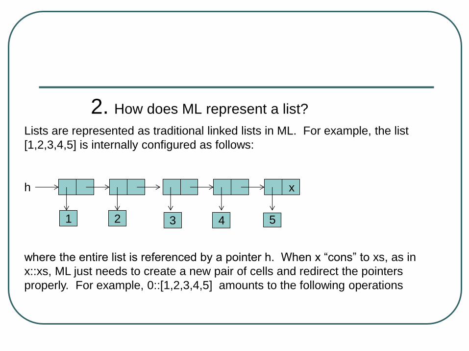
2. How does ML represent a list?

Lists are represented as traditional linked lists in ML. For example, the list

[1,2,3,4,5] is internally configured as follows:

where the entire list is referenced by a pointer h. When x “cons” to xs, as in

x::xs, ML just needs to create a new pair of cells and redirect the pointers

properly. For example, 0::[1,2,3,4,5] amounts to the following operations

x h

1 2 3 4 5

x h

1 2 3 4 5 0

s

x h

1 2 3 4 5 0

create a new pair of cells and

redirect pointer s and h

3. New list-reversal program

note that these operations (creating new cells and redirecting pointers)

take a constant amount of time and are independent of the size of the list

being “con-ed”. This observation gives rise to the following more

efficient program.

fun rev(nil, M) = M

| rev(x::xs, soFar) = rev(xs, x::soFar);

fun revIt(L) = rev(L, nil);

4. Analysis of the new reversal program

rev(x::xs, soFar) = rev(xs, x::soFar)

list of size n list of size n-1 :: takes constant amount

of time

T(0) = a, T(n) = T(n-1) + b

solving this equation leads to T(n) = O(n). That is, the time complexity of

this program is proportional to n, which is better than the time complexity

𝑛2 of the “old” reversal program.

Chapter \lambda calculus basics

(not in the textbook)

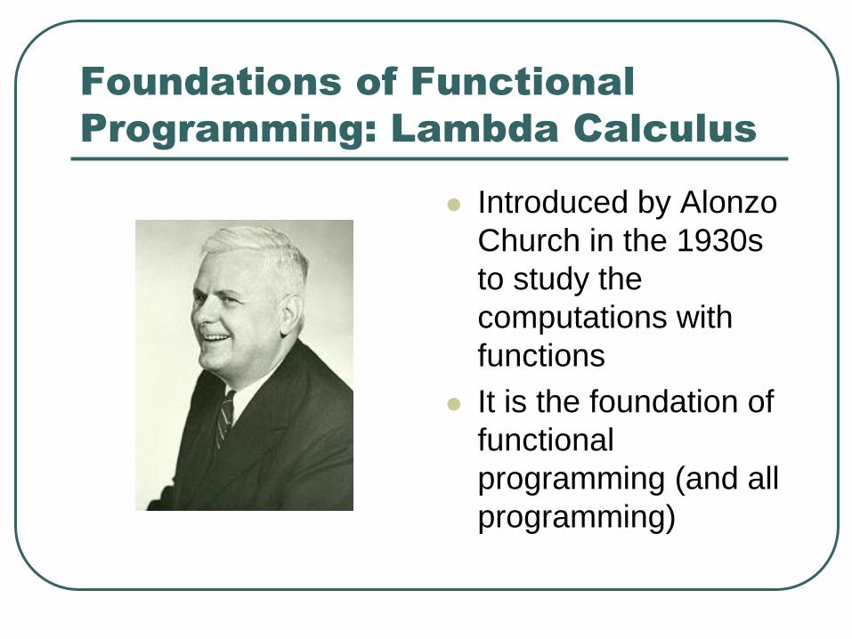
Foundations of Functional

Programming: Lambda Calculus

Introduced by Alonzo

Church in the 1930s

to study the

computations with

functions

It is the foundation of

functional

programming (and all

programming)

Syntax:

• M ::= x | MM | λx.M

• M – term,

• x – variable,

• MM – application,

• λx.M – abstraction

What do we see

here? massive

recursions

Intuitive understanding of abstraction

λ x. M

Binder. It signifies the

variable after it serves as a

parameter (i.e., it binds the

appearance of x in M).

Lambda itself has no

substantial meaning, you

may use any symbol in this

place.

The parameter,

or

bounded variable

The body of the function.

Typically, x appears in M;

but does not have to.

Ex1: x, xx, λx.x, λx.(λy.xy) (pure)

Ex2: λx.(x+1), λy.(y*y+2) (extended, i.e, assume +, 1, 2, * are all defined).

λx.(x+1) basically is the same thing as f where f(x)=x+1.

your own example?

Substitution: • [N/x]M means the result of replacing all

occurrences of x in M by N. (No part of N should be

become bounded in M when M is an abstraction.)

• [N/x]x = N

• [N/x]y = y (if x ≠ y)

• [N/x](PQ) = ([N/x]P)([N/x]Q)

• [N/x](𝜆y.M)= 𝜆𝑦. [N/x]M (𝑥 ≠ 𝑦, y not in N)

Reductions**

• α – axiom : λx.M = λz.[z/x]M (z not in M)

• β – reduction: (λx.M)N = [N/x]M

(underlying ideas of these rules?)

α – axiom says that the function parameter is

not important, we may rename it anyway we

want. (which is exactly the way in which

functions are understood in math)

β – reduction specifies how computation

(using functions) can be carried out.

That’s it. This is all we need. (really?)

Q: do you feel any difference at this

point in terms of the nature of functions

between math and this lambda

calculus?

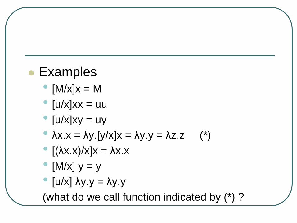
Examples

• [M/x]x = M

• [u/x]xx = uu

• [u/x]xy = uy

• λx.x = λy.[y/x]x = λy.y = λz.z (*)

• [(λx.x)/x]x = λx.x

• [M/x] y = y

• [u/x] λy.y = λy.y

(what do we call function indicated by (*) ?

• Conventions:

• Applications associate to the left. That is: MNP

abbreviates (MN)P

• Bodies of abstractions are as far as possible to

the right. E.g.:

λx. λy. xyx stands for λx.(λy.(xyx))

• λxy.M is an abbreviation for λx.λy.M

What does λx.λy.M mean intuitively?

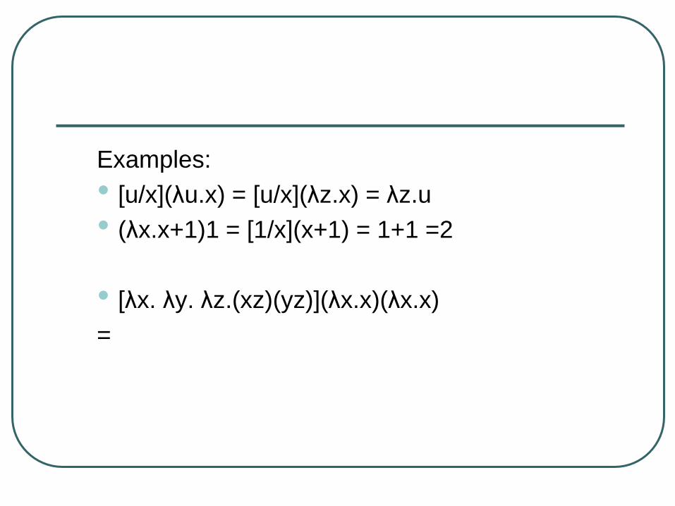
Examples:

• [u/x](λu.x) = [u/x](λz.x) = λz.u

• (λx.x+1)1 = [1/x](x+1) = 1+1 =2

• [λx. λy. λz.(xz)(yz)](λx.x)(λx.x)

=

Examples:

• [u/x](λu.x) = [u/x](λz.x) = λz.u

• (λx.x+1)1 = [1/x](x+1) = 1+1 =2


= (λy.λz.((λx.x)z)(yz))(λx.x) (𝛽 rule, abc=(ab)c)

Examples:

• [u/x](λu.x) = [u/x](λz.x) = λz.u

• (λx.x+1)1 = [1/x](x+1) = 1+1 =2


= (λy.λz.((λx.x)z)(yz))(λx.x)

= (λy.λz.(z)(yz))(λx.x) (𝛽 rule)

Examples:

• [u/x](λu.x) = [u/x](λz.x) = λz.u

• (λx.x+1)1 = [1/x](x+1) = 1+1 =2



= (λy.λz.(z)(yz))(λx.x)

= λz.z((λx.x)z) (𝛽 rule)

Examples:

• [u/x](λu.x) = [u/x](λz.x) = λz.u

• (λx.x+1)1 = [1/x](x+1) = 1+1 =2



= (λy.λz.(z)(yz))(λx.x)

= λz.z((λx.x)z)

= λz.zz

what does this mean?

z applied to itself?


evaluate it in

another way





= λz. ((λx.x)z) ((λx.x)z)



= λz. ((λx.x)z) ((λx.x)z)

= λz. zz

note: two computations have different order but

have the same result. (<diamond property> as

shown on the next slide)

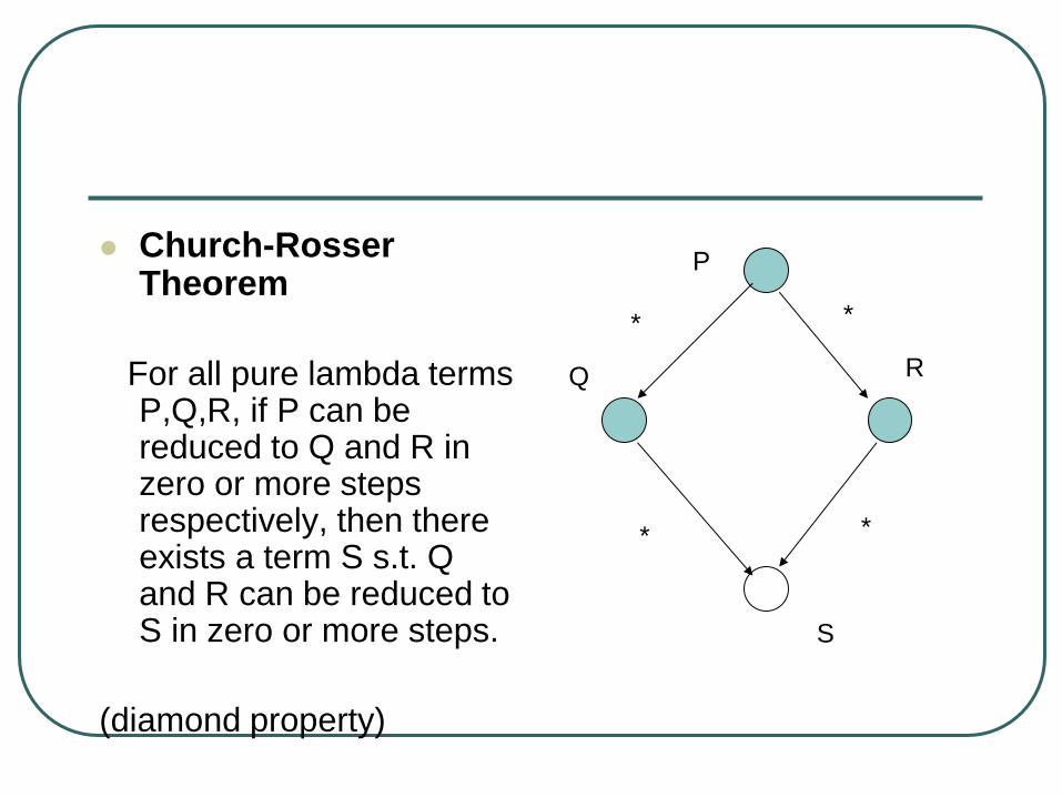
Church-Rosser Theorem

For all pure lambda terms P,Q,R, if P can be reduced to Q and R in zero or more steps respectively, then there exists a term S s.t. Q and R can be reduced to S in zero or more steps.

(diamond property)

P

Q R

S

*

* *

*

Non-terminating reductions

• ex1: (λx.xx)(λx.xx)

= (λx.xx)(λx.xx)

= …….

Def: if a value v satisfies f(v)=v for a function f,

then v is called a “fix point” (or fixed point) of f.

• ex2: let Y = λf. (λx.f(xx)) (λx.f(xx))

then, Yf = (λx.f(xx)) (λx.f(xx))

= f ((λx.f(xx)) (λx.f(xx)))

= f (Yf)

so, Yf is a fix point of f. Y is called the fix

point operator (of f, for any f).

Ex: evaluate the lambda term

[λf.λx.f(f(fx))] [λg.λy.g(gy)] [λz.z+1] 0

Let P = λf.λx.f(f(fx))

Q = λg.λy.g(gy)

S = λz.z+1

Then, we need to evaluate the term PQS0

PQS0

= Q(Q(QS))0 (why?) -------- (1)

Let M = Q(QS), then

(1) = QM0

= M(M0) (why?) ----------- (2)

(ok, let’s figure out what M0 is)

M0 = Q(QS)0

= (QS)(QS0)

= (QS)(S(S0))

= (QS)(S1) (S0 = (λz.z+1)0 = 1)

= (QS)2

= S(S2)

= S3

=4

So, (2) = M4

= Q(QS)4

= (QS)(QS4)

= (QS)(S(S4))

= (QS)6

= S(S6)

= 8

Hence, PQS0 = 8

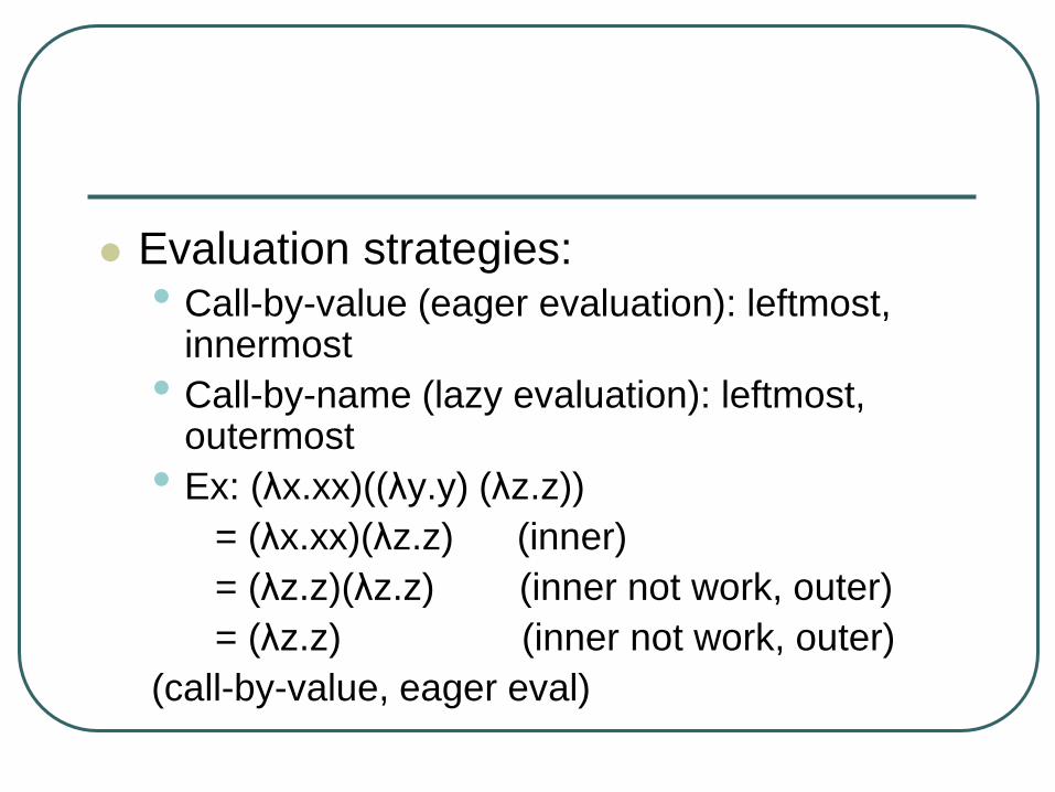
Evaluation strategies: • Call-by-value (eager evaluation): leftmost,

innermost

• Call-by-name (lazy evaluation): leftmost, outermost

• Ex: (λx.xx)((λy.y) (λz.z))

= (λx.xx)(λz.z) (inner)

= (λz.z)(λz.z) (inner not work, outer)

= (λz.z) (inner not work, outer)

(call-by-value, eager eval)

• (λx.xx)((λy.y) (λz.z))

= ((λy.y)(λz.z)) ((λy.y)(λz.z)) (outer)

= (λz.z)((λy.y)(λz.z)) (outer not work, inner)

= (λy.y)(λz.z) (outer)

= λz.z (outer)

(call-by-name, lazy eval)

An applied Lambda Calculus

• M ::= c | x | M1M2 | λx.M ( c – constants)

• c ::= true | false | if | 0 | iszero | pred | succ |fix

• Ex: as such, a term of applied λ calculus is

( ( ( if x) y) true )

which can be abbreviated as

if x y true

Q: by the grammar of applied lambda

calculus, is

true false

a legitimate term? If so, what does it

mean?

Reduction rules for constants

• if true M N = M

• if false M N = N

• fix M = M (fix M) (strange?)

• iszero 0 = true

• iszero (succk 0) = false (k >=1)

• iszero (predk 0) = false (k >= 1)

• (see next slide for this “power” notation)

• succk M is an abbreviation for

succ(succ(….(succ M))))..))

where succ is applied k times to M. (Note: There is

actually no such a “power” construct in the applied

lambda calculus we study. ) We choose to use such

an abbreviation b/c otherwise we will be running out

of the edge of the paper when writing long lambda

terms……

Ex: succ2M means succ(succ M)

succ3M means succ(succ(succ M))

• pred(succ M) = M

• succ(pred M) = M

Moreover, we can intuitively regard:

• 0 0

• succ 0 1

• succ (succ 0) = succ2 0 2

• pred 0 -1

• pred(pred 0) = pred2 0 -2

Ex:

(λx. if x 0 (succ 0) ) false

= if false 0 (succ 0)

= succ 0

= 1 (informally)

ML core (ML0) is a syntactically sugared applied

lambda calculus

Lambda Cal ML0

x x

c c

MN MN

λx.M fn x => M

succk 0 k

predk 0 -k

if P M N if P then M else N

(λx.M)N let val x=N in M

(λf.M)(fix (λf.λx.N)) let rec fun f(x)=N in

M

Relationship between recursive

functions and fixed point

f(x) = ….f… f recursively defined

f(x) = M[f] syntactic hole

f = λx.M[f] writing f in lambda notion

= (λg.λx.[g/f]M)f

f = Ff f is the fix pt of F, where

F = λg.λx.[g/f]M

f or f(x)

Note: f is not the same as f(x)

(recall the one of the hw problems we did

before)

e.g. given f(x) = x+1

how to appreciate the difference among f, f(x),

and x+1?

why?why?why?why?

f is the function (itself)

f(x) is the element in the codomain to

which x is mapped under f (not the f

itself), in terms of math.

in terms of programming, f(x) is the value

returned by the function f (not the

function itself) when x is submitted to f

ex: A = {1,2,3}, B = {2,3,4}

f is a function from A to B, (and its

behavior) is specified by

f(x) = x+1 x in A

then,

f(1) = 2, f(2) = 3, f(3) =4

Can we derive the meaning of f(k) or f(x)?

Can we write out f (again, the function

itself, not f(x) or f x) directly/indirectly?

• In traditional math?

• In lambda calculus?

• (left as hw?)

How to “define” recursive functions

w/o using function names?

Fixed pt answers the question

Ex: x + y =

y if x=0

(one less then x) + (one more than y) ,

otherwise

+ is defined recursively (why?)

define the operation + using fix point

notation

plus x y =

y if iszero x

plus (pred x) (succ y) otherwise

plus = λxy. if (iszero x) y (plus (pred x) (succ y))

= (λf. λxy. if (iszero x) y (f (pred x) (succ y)) ) plus

then plus = fix (λf. λxy. if (iszero x) y (f (pred x) (succ y)) )

This is the definition of plus w/o using any name.

Rewriting plus, we have

Understand how the reduction

rule fix M=M(fix M) works

The rule fix M = M (fix M) is natural, b/c it

just says t = M t where t = fix M, which is

the def of fixed pt.

a concrete example to how this rule

really works

let f(n) = if n=0 then 1 else n*f(n-1)

= if n=0 1 n*f(n-1) (simplified a bit w/o syntactic sugar)

i.e. f = 𝜆n. if n=0 1 n*f(n-1)

f = fix (𝜆d. 𝜆n. if n=0 1 n*d(n-1)) = fix M

where M = 𝜆d. 𝜆n. if n=0 1 n*d(n-1)

f 2 = (fix M) 2

= M (fix M) 2

= if 2=0 1 2*[(fix M)(1)] (recall M= 𝜆d. 𝜆n. if n=0 1 n*d(n-1) )

= 2*[(fix M)(1)]

= 2*[ M (fix M) 1]

= 2*[ if 1=0 1 1*(fix M)(0) ]

= 2*[ 1* [(fix M)(0)] ]

= 2*[ 1* [M (fixM) 0] ]

= 2*[ 1* [if 0=0 1 0*(fix M)(-1) ] ]

= 2*[ 1* 1]

= 2

assuming all relevant operations and numbers are defined in the applied

lambda calculus in this example)

Typed Lambda Calculus

Syntax for types

• 𝜏 ∷= 𝑘 | 𝜏1 → 𝜏2

k: ground types (such as, int, bool, real, etc.)

𝜏1 → 𝜏2 : function type (as we see in ML)

Function type example: int -> int, int->(int->bool)

Syntax for terms:

•𝑀 ∷= 𝑥 𝑀𝑁 𝜆 𝑥: 𝜏 .𝑀

note the appearance of type after the binder

Type Checking Rules

• Γ is the type assignment context/environment

• Γ = {𝑥1: 𝜎1, 𝑥2: 𝜎2, … , 𝑥𝑛: 𝜎𝑛}

Γ ∪ 𝑥 ∶𝜎 ⊢ 𝑥 ∶ 𝜎 (variable)

Γ ⊢ 𝑀∶ 𝜎→𝜏 Γ ⊢ 𝑁∶𝜎

Γ ⊢ 𝑀𝑁 ∶ 𝜏 (application)

Γ∪ 𝑥:𝜎 ⊢ 𝑀 ∶ 𝜏

Γ ⊢ 𝜆 𝑥:𝜎 .𝑀 ∶ 𝜎→𝜏 (abstraction)

How to read these rules?

• 𝐴 ⊢ 𝐵 means “A implies B.”

• 𝐴

𝐵 means “if A holds, then B holds”.

• So we have two different levels of

implications. They are standard first-order

logical implications. (what we learned in

discrete math.)

• Ex: show ∅ ⊢ 𝜆 𝑥: 𝑖𝑛𝑡 . 𝑥 ∶ 𝑖𝑛𝑡 → 𝑖𝑛𝑡

∅ ∪ 𝑥: 𝑖𝑛𝑡 ⊢ 𝑥: 𝑖𝑛𝑡 𝑣𝑎𝑟

∅ ⊢ 𝜆 𝑥: 𝑖𝑛𝑡 . 𝑥 ∶ 𝑖𝑛𝑡 → 𝑖𝑛𝑡(abs)

• Ex: show ∅ ⊢ 𝜆 𝑥: 𝑎 . 𝜆 𝑦: 𝑏 . 𝑥 ∶ 𝑎 → (𝑏 → 𝑎)

∅ ∪ 𝑥: 𝑎 ∪ 𝑦: 𝑏 ⊢ 𝑥: 𝑎(𝑣𝑎𝑟)

∅ ∪ 𝑥: 𝑎 ⊢ 𝜆 𝑦: 𝑏 . 𝑥 ∶ 𝑏 → 𝑎 𝑎𝑏𝑠

∅ ⊢ 𝜆 𝑥: 𝑎 . 𝜆 𝑦: 𝑏 . 𝑥 ∶ 𝑎 → (𝑏 → 𝑎)(abs)

Polymorphic Types (2nd

order

Typed Lambda Calculus)

Motivation

• For the identity function 𝜆𝑥. 𝑥

𝜆𝑥. 𝑥 1 = 1

𝜆𝑥. 𝑥 𝜆𝑥. 𝑥 + 1 = 𝜆𝑥. 𝑥 + 1

Then, how do we type this thing 𝜆𝑥. 𝑥?

(assume 1, 2, …, +, -, … are part of the syntax)

Syntax:

• Types:

𝑃𝑇 ∷= 𝜏 | type expression

∀𝑡. 𝑃𝑇 polymorphic type

𝜏 ∷= 𝑏 | ground type

𝑡 | type variable

𝜏 → 𝜏 function type

• Terms:

•𝑀 ∷= 𝑥 | variable

𝑀𝑁 | application

𝜆 𝑥: 𝜎 .𝑀 | abstraction

𝑀𝜎 | type application

Λ𝑡.𝑀 type abstraction

(note that types can be abstracted and instantiated

now. In a sense, types are gaining an “equivalent”

status w/ terms)

• Corresponding to the two new terms type

application and type abstraction, we have the

following typing rules

• Γ ⊢ 𝑀 ∶ ∀𝑡.𝑃𝑇

Γ ⊢ 𝑀𝜏 ∶ 𝜏 /𝑡 𝑃𝑇 ( type application)

• Γ ⊢ 𝑀 ∶ 𝑃𝑇

Γ ⊢ Λ𝑡.𝑀 ∶ ∀𝑡.𝑃𝑇 (type abstraction)

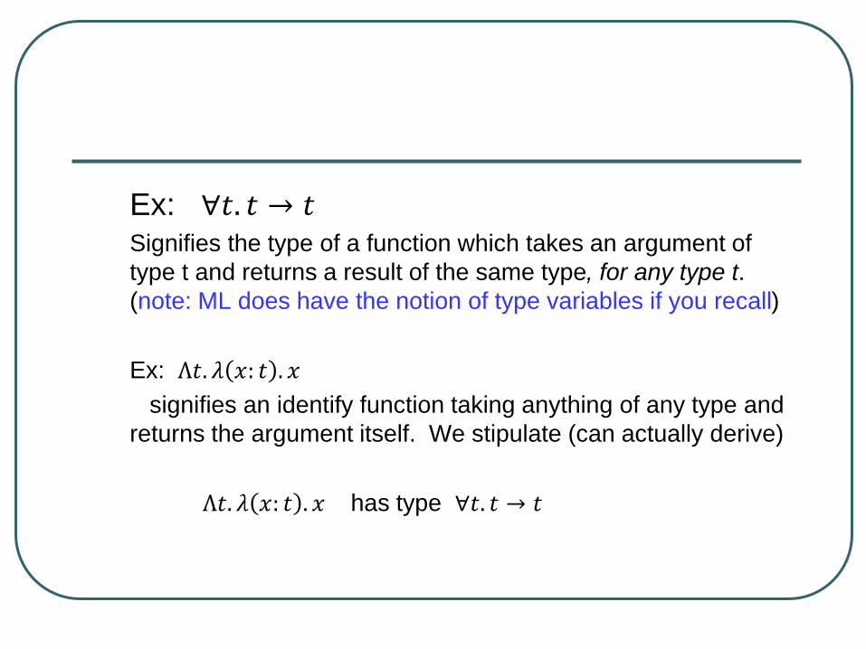
Ex: ∀𝑡. 𝑡 → 𝑡 Signifies the type of a function which takes an argument of

type t and returns a result of the same type, for any type t.

(note: ML does have the notion of type variables if you recall)

Ex: Λ𝑡. 𝜆 𝑥: 𝑡 . 𝑥

signifies an identify function taking anything of any type and

returns the argument itself. We stipulate (can actually derive)

Λ𝑡. 𝜆 𝑥: 𝑡 . 𝑥 has type ∀𝑡. 𝑡 → 𝑡

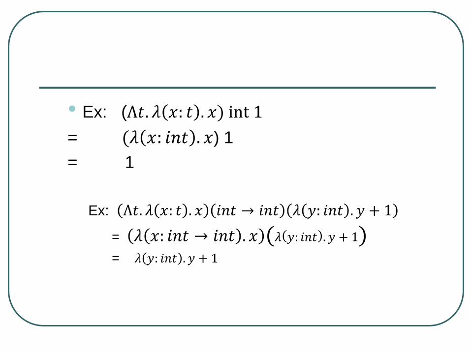
• Ex: (Λ𝑡. 𝜆 𝑥: 𝑡 . 𝑥) int 1

= (𝜆 𝑥: 𝑖𝑛𝑡 . 𝑥) 1

= 1

Ex: Λ𝑡. 𝜆 𝑥: 𝑡 . 𝑥 𝑖𝑛𝑡 → 𝑖𝑛𝑡 𝜆 𝑦: 𝑖𝑛𝑡 . 𝑦 + 1

= 𝜆 𝑥: 𝑖𝑛𝑡 → 𝑖𝑛𝑡 . 𝑥 𝜆 𝑦: 𝑖𝑛𝑡 . 𝑦 + 1

= 𝜆 𝑦: 𝑖𝑛𝑡 . 𝑦 + 1

Ex: Λ𝑡. 𝜆 𝑓: 𝑡 → 𝑡 . 𝜆 𝑥: 𝑡 . 𝑓(𝑓𝑥) : ∀𝑡. 𝑡 → 𝑡 → (𝑡 → 𝑡)

Λ𝑡. 𝜆 𝑓: 𝑡 → 𝑡 . 𝜆 𝑥: 𝑡 . 𝑓(𝑓𝑥) 𝑖𝑛𝑡 𝑠𝑢𝑐𝑐 0

= 𝜆 𝑓: 𝑖𝑛𝑡 → 𝑖𝑛𝑡 . 𝜆 𝑥: 𝑖𝑛𝑡 . 𝑓(𝑓𝑥) 𝑠𝑢𝑐𝑐 0

= 𝜆 𝑥: 𝑖𝑛𝑡 . 𝑠𝑢𝑐𝑐 𝑠𝑢𝑐𝑐 𝑥 0

= 𝑠𝑢𝑐𝑐 𝑠𝑢𝑐𝑐 0

(= 2)

Denotational/Mathematical

Semantics of Lambda Calculus

Dana Scott: founder of

denotational/mathematica

l semantics of

programming languages.

Frist person who

successfully gives a

mathematical

interpretation of

programming language

meanings.

Idea: (we only scratch the surface of it)

Syntactic domain Semantic domain

Language

constructs,

programs

Mathematical

meanings of those

“symbols” on the left

Semantic function maps

syntax to semantics

For the simply typed lambda calculus

covered before

Syntax for types

𝜏 ∷= 𝑘 | 𝜏1 → 𝜏2

Syntax for terms:

𝑀 ∷= 𝑥 𝑀𝑁 𝜆 𝑥: 𝜏 .𝑀

Its “set-and-function” semantics is given

as follows:

• For types

• 𝑘 = 𝐴 where 𝐴 is a (non-empty) set.

• 𝜏1 → 𝜏2 = 𝜏2𝜏1

( i.e., the set of all functions from

the set 𝜏1 to the set 𝜏2 . )

Ex: (given 𝑘 = 𝐴 )

• 𝑘 → (𝑘 → 𝑘)

is the set of functions which map an element in A to

a function from A to A.

• (𝑘 → 𝑘) → 𝑘

is the set of functions which map a function from A to

A to an element in A.

• For terms,

• let 𝜌 be a function from the set of all variables to

the union of their semantic domains.

•𝜌[𝑥 ↦ 𝑑] means a function that works just like 𝜌 if the argument to it is not x; if the argument is x, then

it returns d. That is,

• 𝜌 𝑥 ↦ 𝑑 𝑦 = 𝑑 𝑦 = 𝑥

𝜌 𝑦 𝑜𝑡ℎ𝑒𝑟𝑤𝑖𝑠𝑒

• Then, terms are interpreted under 𝜌

• 𝑥 𝜌 = 𝜌 𝑥 ∈ 𝜏 where 𝜏 is the type of 𝑥

• 𝜆 𝑥: 𝜏 .𝑀 𝜌 = 𝑓: 𝜏 → 𝜎

where 𝜏 → 𝜎 is the type of 𝜆 𝑥: 𝜏 .𝑀 and 𝑓 is

given by, for any 𝑑 ∈ 𝜏 ,

𝑓 𝑑 = 𝑀 (𝜌 𝑥 ↦ 𝑑 )

• 𝑀𝑁 𝜌 = 𝑀 𝜌 ( 𝑁 𝜌)

where 𝜏 is the type of N

Ex: • 𝜆 𝑥: 𝜏 . 𝑥 ∶ 𝜏 → 𝜏 𝜌 is function 𝑓 ∶ 𝜏 → 𝜏

where

𝑓 𝑑 = 𝑥: 𝜏 (𝜌 𝑥 ↦ 𝑑 )

= (𝜌[𝑥 ↦ 𝑑]) 𝑥

= d

that is, the semantics of this lambda expression is

the identify function from some set to the same set.

Ex: • 𝜆 𝑥: 𝜏 . 𝑥 𝑥 ∶ 𝜏 𝜌

= ( 𝜆 𝑥: 𝜏 . 𝑥: 𝜏 → 𝜏 𝜌) ( 𝑥: 𝜏 𝜌)

= 𝑓 ( 𝑥: 𝜏 𝜌) (f is the identify function from previous example)

= 𝑓(𝜌 𝑥 )

= 𝜌 𝑥

That is, the meaning of this program is whatever the

meaning of the variable x. (which is, indeed, the way

the program works)

Chapter 4

Input and output

1 . Type unit

unit is an ad hoc and “man-made” type in ML. It

was created to solve some purely technical issues.

Its sole value is (). Most side-effect functions are

typed using unit.

2. The print function

• Syntax: print<string>

• Type: string -> unit

• Semantics: send the value of the string to the

“standard out” (in the sense of Unix) which is the

terminal by default.

• Ex:

or,

Q: When submitting an argument to the

function print, does ML allow us an option to

either put the argument inside () or not? Or,

ML always takes a “naked” argument when it

is submit to a function?

What do you think?

Q2 (about the print function)

• what does it return?

• what does it do?

3. Sequencing

• This construct has a strong flavor of

imperative programming; but it is still an

expression.

• Syntax:

• ( <exp1>;

<exp2>;

….

<expn>)

• Semantics:

each <exp_i> is evaluated in turn. The value of the

last expression is used as the value of the entire

expression. (This has a “being forced” flavor.)

Ex:

• Ex:

Q: what is the value of the expression above?

Another question:

• Isn’t ( ) the operator for constructing tuples? If

so, how come it is used to make sequences

here?

4. Reading From a File • Note: some of the facilities regarding the reading

from files are changed in newer versions of

SML/NJ. The text was written with its “current-

time” version of SML/NJ.

• Open the TextIO structure

• Syntax: open TextIO;

• Semantics: It brings up all the functions in TextIO to

the top level environment so that they can be called

w/o “dot” through the structure name.

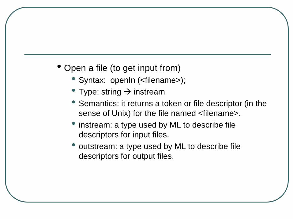
• Open a file (to get input from)

• Syntax: openIn (<filename>);

• Type: string instream

• Semantics: it returns a token or file descriptor (in the

sense of Unix) for the file named <filename>.

• instream: a type used by ML to describe file

descriptors for input files.

• outstream: a type used by ML to describe file

descriptors for output files.

• ex:

• Ways to read from a file

• read 1 character

• syntax:

• input1 (<fileid>)

• type

• instream elem option

• (here, elem is the same as char)

• semantics

• consumes one character from the file (specified by

<fileid>), returns that character with type elem

option, and move the pointer one position to the

right (towards the end of the file).

• ex: suppose “t.txt” contains

[23,34)

123, 45

• Here, option is a very interesting (new) type

constructor: it takes some type, say T, and gives

you back another type: T option. It works, in a

sense, in the similar way as the list type

constructor. Its values are either SOME

<something> or NONE, where SOME and NONE

are data constructors. In particular, SOME takes

some argument, but NONE takes no argument.

more ex:

Q: how these are

connected to the

theory of 2nd order

typed lambda

calculus? Do you see

the connection?

• read a few char

• syntax:

• inputN(<fileid>, n)

• type: instream * int vector

• (here, vector is the same as string)

• semantics: consumes the next n characters from

the file and return them as a string.

• ex:

• read an entire line

• syntax:

• inputLine(<fileid>)

• type: instream vector option


• semantics: consumes the entire line and returns it

as a string option.

• ex:

• read the entire file

• syntax:

• input(<fileid>)

• type: instream vector


• semantics: consumes the entire file and returns it

as a string.

• ex:

Chapter 5 Functions Again

Matches

• Syntax

<p1> => <e1> | <p2> => <e2> |… | <pn> => <en>

where <pi> are patterns and <ei> are expressions.

• Semantics

• when a match is applied to some value, all patterns

will be checked in the existing order, until a match

is found. Then the corresponding exp will be

evaluated and (under the bindings of the match)

and the result is the result of this match

expression. Match should/must be exhaustive.

• ex: define anonymous functions

or

this gives the 𝜆-way to define functions. The

primary use of matches is w/ case expressions.

ex:

Case expressions

• Syntax:

• case <exp> of <match>

• Semantics

• <exp> is evaluated to a value. <match> is applied

to the ensuing value, and the result of <match>

expression is the result of the case expression.

• ex: (next slide)

• Ex:

Exceptions

• Exceptions provide structured way of handling

“bad” situations. For some of what can be

done by exceptions, they can also be done

w/o exceptions, but exceptions give a more

“elegant” way out.

• Exceptions are treated as values in ML and

have type exn.

• Define exceptions

• Syntax

• exception <identifier> [ of <type>]

• Semantics

• declares <identifier> to be an exception; or, we say

that <identifier> constructs an exception.

• In case w/ <type>, the <identifier> constructs an

exception taking a parameter of type <type>. That

is, the <identifier> is an exception constructor in this

case.

• Ex:

• Raise exception

• syntax

• raise <exn-id> [value]

• semantics

• signals that exception <exn-id> [value] has

occurred.

• ex:

• see next example

• Handle exceptions

• Syntax

• <exp> handle <match>

where <exp> is the place where possible exception

might occur.

• Semantics

• if no exception is raised in <exp>, then the value returned

by <exp> is the value of this handling expression;

otherwise, the exception raised in <exp> is submitted to

<match>, and the value returned by <match> is the result

of this exception-handling expression. As such, the type of

<exp> and the type of expressions in <match> must be

the same.

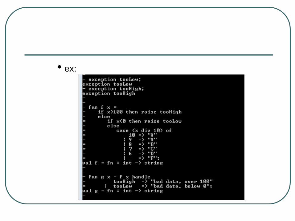
• ex:

Polymorphic Functions

• We say a function is polymorphic is it can take

many different types of arguments as inputs.

• Polymorphism is natural and “easy” and

powerful in functional programming; but it may

not be the case in imperative programming.

(Does C support polymorphism? What about

Java?...)

Polymorphic Functions

• Polymorphism may be best understood with

the framework of lambda calculus in your

mind. That is, if you understand lambda

calculus well, then ML polymorphism would

seem to be just natural and automatic.

• Therefore, theory is important.

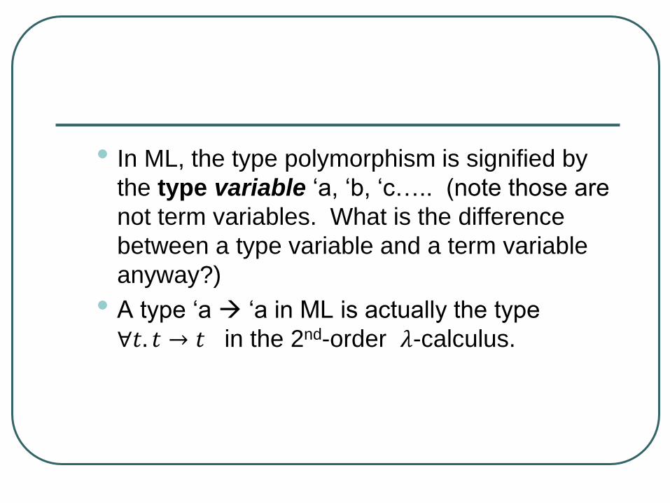
• In ML, the type polymorphism is signified by

the type variable ‘a, ‘b, ‘c….. (note those are

not term variables. What is the difference

between a type variable and a term variable

anyway?)

• A type ‘a ‘a in ML is actually the type

∀𝑡. 𝑡 → 𝑡 in the 2nd-order 𝜆-calculus.

Ex:

• The well-known identity function. It takes

anything (of any type) and returns that same

thing (of the same type).

• Ex: the list reversal function we studied

before. Its type is ‘a list ‘a list

But, there are issues

• Ex: how about id applied to itself since id has

a polymorphic type?

• To understand this, we need to know the

following

• In ML, the fine meanings of type variables can

be distinguished by so called generalizable

and non-generalizable type variables. Also,

there are expansive and non-expansive

expressions in ML which are coined to deal

with typing issue – determination of types at

compile time. (see p145 for explanation of

these concepts)

• In summary,

• Stipulation: type variables (if any) in the type of top-

level expressions must be generalizable.

• If the expression is non-expansive, then things are

fine in the sense that type variables are allowed in

the type of the expression, and they are all

generalized.

• If the expression is expansive, then be careful

about those type variables that are non-

generalizable, which cannot be allowed to appear

in the type the final result.

• Nonetheless, the problem with id(id) in ML

can be better understood using lambda

calculus (left as part of hw).

• The rest examples in the book are all

centralized around this “id(id)” issue. Once

you truly understand why “id(id)” gives an

error, you will understand these instances

with an ease.

Higher order functions

• A function is said to be of higher order if

functions can be served as input and/or

output of this function.

• Again, higher-order functions can be best

understood w/ the lambda calculus

framework in your mind.

• In lambda calculus, anything can be used as

an input to a function; so of course, a function

can be an input to a function. Output is in a

similar situation.

Three exemplifying higher-order

functions

• mapall: it takes a function f and list

[𝑣1, 𝑣2, … , 𝑣𝑛] as inputs (in a rough, or

inaccurate sense) and returns

[𝑓𝑣1, 𝑓𝑣2, … , 𝑓𝑣𝑛] as the result.

Q: regarding the “rough” or “inaccurate”

remark for mapall, what would be the

“accurate” explanation?

Connection to lambda calculus?

• ex:

• ex:

• ex:

• doitall: it takes a binary function f and list of

elements [𝑣1, 𝑣2, … , 𝑣𝑛] and returns

𝑓(𝑣1, … 𝑓 𝑣𝑛−2, 𝑓 𝑣𝑛−1, 𝑣𝑛 …) as the result.

• Ex

• Ex

• filter: it takes a predicate p and a list of

elements and returns the list of elements

obtained by deleting those elements that do

not satisfy p.

• Ex:

• Ex:

Curried functions

• This term, again, comes from lambda

calculus.

• In (pure) lambda calculus, there is no notion of

pairs, and there is always one variable after the

binder lambda. So, it seems that there is a

“trouble” to express the situation of functions that

take more than one parameters.

• But, functions of multiple parameters can be

regarded or “encoded” equivalently as (higher)

order functions that take only one parameter.

• ex: Let f be defined by f(x,y)=x+y. The f can be

encoded as 𝜆𝑥. 𝜆𝑦. 𝑥 + 𝑦 (assume + operation is

defined here. Also note that this is a higher order

function). To see this encoding is right, note the

fact that

f(k,m) = k+m

𝜆𝑥. 𝜆𝑦. 𝑥 + 𝑦 𝑘𝑚 = k + m

(note the rightmost is the result of two beta

reductions. That is, two applications occur)

In ML, the actual code would be

Note: although f and f1 can work equivalently (to some extent), they

DO have different types. The type of f is int*int -> int whereas the

type of f1 is int -> (int->int), and f1 3 is a partially instantiated

function from int to int.

• ML style of function application is to drop the

() around the argument. E.g. , write f x instead

of f(x).

• Again, this style is influenced by lambda

calculus. In lambda calculus, we typically

write MN for application, not M(N). (right?)

Built-in Higher Order Function

The only thing that is new to us is probably the

function foldr (foldl is his “sister”), which is

defined as

foldr takes three arguments: a binary function f,

an initial value b, and a list [𝑣1, 𝑣2, … , 𝑣𝑛−1, 𝑣𝑛], and returns

𝑓(𝑣1, … , 𝑓 𝑣𝑛−1, 𝑓 𝑣𝑛, 𝑏 …)

It is somehow similar to the “doitall” function

covered before, but takes a different number of

arguments.

Ex: sum of an int list

• Length of a list

Chapter 6 Defining Your Own Types

Type Synonyms

Syntax

• type (list of para) <new id> = <old ty exp>

Semantics:

• give an existing type a new name. (and this

feature is not very exciting, (my opinion))

ex:

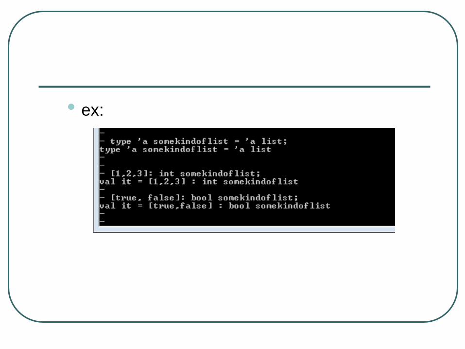
• ex:

Datatype

• Note: the book deliberately groups the two

words “data” and “type” into one word.

Consequently, the phrase “datatype” and

“data type” have (subtle) different meanings.

Do not confuse them, (at least in the study of

the ML language).

• Here, the term “datatype” involves two layers

of meanings: (1) data and (2) type. The the

definition of a datatype in ML correspondingly

• gives you the meanings on these two aspects.

Syntax

• datatype (list of para) <id> =

<constructor exp1> |

<constructor exp2> |

….

<constructor expn> ;

Semantics:

• a new type (or type constructor) <id> is

defined.

• the values (i.e. data) which are of this newly

defined type are given in the group of

<constructor expi> through data constructors.

ex:

• here, myFamily is the newly defined type and

its value set is {Mom, Dad, Al, Mary}.

• things become more interesting when type

parameters are involved in datatype

definitions. And the role of type constructor and

data constructor can be seen clearly in this

case.

ex:

in this example, family is the type constructor

(taking a type and returns another type) and Al,

Mary, Dad, Mom are all data constructors

(taking some data and return some data).

another ex:

type constructor: slT;

data constructors: S and L

Recursive datatypes

• The typical and most useful example here is

the coding of binary trees.

• Binary trees are defined regularly (i.e. in the

inductive manner as we see in data structures

– empty tree, left subtree, right subtree…)

• the type for binary can be defined as

• Then, the following are binary trees:

• (1)

which can be pictured as (the empty tree)

• (2)

which can be pictured as

0

• (3)


0

/ \

1 2

• (4)


0

/ \

1 2

/ \

3 4

Binary Search Trees (BSTs)

DEF:

For any node in the tree, its value is

larger than the value of every node in the

left subtree, and less than the value of

every node in the right subtree

Binary Search Trees (BSTs)

DEF: For any node in the tree, its value is

larger than the value of every node in the left

subtree, and less than the value of every

node in the right subtree

Ex: 4

2 6

1 3 5 7

def of binary

tree type

the “<“ function

the lookup

function

an int BST

search the

BST for 4

and 9

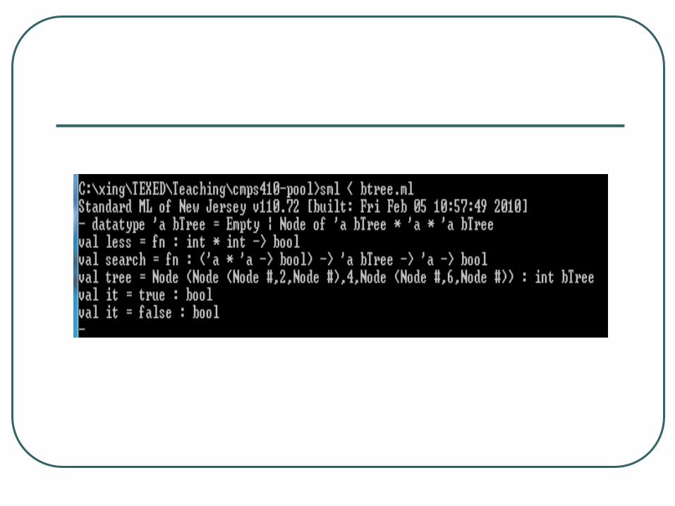
Ch 7: Imperative Features of ML

Arrays

• Array is an imperative notion. It does not

directly “fit” into functional programming style.

• As an additional data structure, arrays is

added to ML due to efficiency reasons. (That

is, there are some situations where no

adequately efficient programs can be done w/

ML’s list, so we have to resort to arrays.)

Three basic things to know:

• How to create an array?

• How to access an array element?

• How to change an array element?

• There is an Array structure in ML where all array

facilities can be found. So open this structure first.

• From the resulting list of opening Array structure,

note particularly the following functions

• array : int * ‘a ‘a array

• sub : ‘a array * int ‘a

• update : ‘a array * int * ‘a unit

• These three functions are the solutions to the three

issues : how to create/access/change an array

(element)?

• Note: interestingly, everything about array is done

via functions.

• examples

yes, array is a function. It takes two parameters n of int and x of

any type and returns an array of size n w/ every element in the

array initialized to x. Note the notation of the type of an array is

similar to that of a list.

• a subtle point: since ‘a array represents the

type of an array, we can regard array as a

type constructor in the same sense that list is

a type constructor b/c ‘a list means the type of

a list. However, array, as we have seen, is

indeed an array-constructing function, while

list cannot be used a list-constructing function.

• although ML uses [| …. |] in its response to creation

of an array, it does appear that [|…|] is actually an

array constructor. That is, things like [| 2, 3 |] may

not give you an array.

The fact that arrays can’t be easily constructed as

lists suggest that they may not be used in the way

lists are used. In particular, you may not want to

return an array in a function as the result; instead,

you may want to pass arrays as parameters around,

and make changes to the array as side effects.

• ex (cont.)

ch 8 Structures

Structures

same idea as ADT

allows information hiding

close to the notion of object (but not the

same)

a combination of data, types, and

operations; a package of elements

needed for some programming

ex:

create a point (0,0)

set this point’s x field (the

result is another point)

set this point’s y data field

(the result is another new

point)

syntax: structure is declared by

structure <id> =

struct

some def;

some def;

…..

some def;

end

Signature

signature is the “type” a structure

signature could be defined

independently of structures

can be used to restrict structures

Documents

Introduction to Functional Programming with SML to Functional Programming with SML Dr. Cong-Cong Xing Dept of Mathematics and Computer Science . ... If there are any issues that need