Introduction to Financial Engineering Aashish Dhakal Week 5: Black Scholes Model

Introduction to Financial Engineering

Aashish Dhakal

Week 5: Black Scholes Model

Pricing of Option : Black – Scholes Model

B & S give the valuation model of call option.

Before moving into the valuation of CALL using B & S and use of same for deriving the value of PUT lets see traditionally, how we calculate the Gross PAY Off (gross value) in CALL.

CALL Right to BUY

And, We always BUY at LOW.

So, For us to exercise a CALL option, Option must provide us an offer to buy at LOW.

I.e. Option must be In The Money.

And, our Gain = Market Price – Strike Price = (S – E)


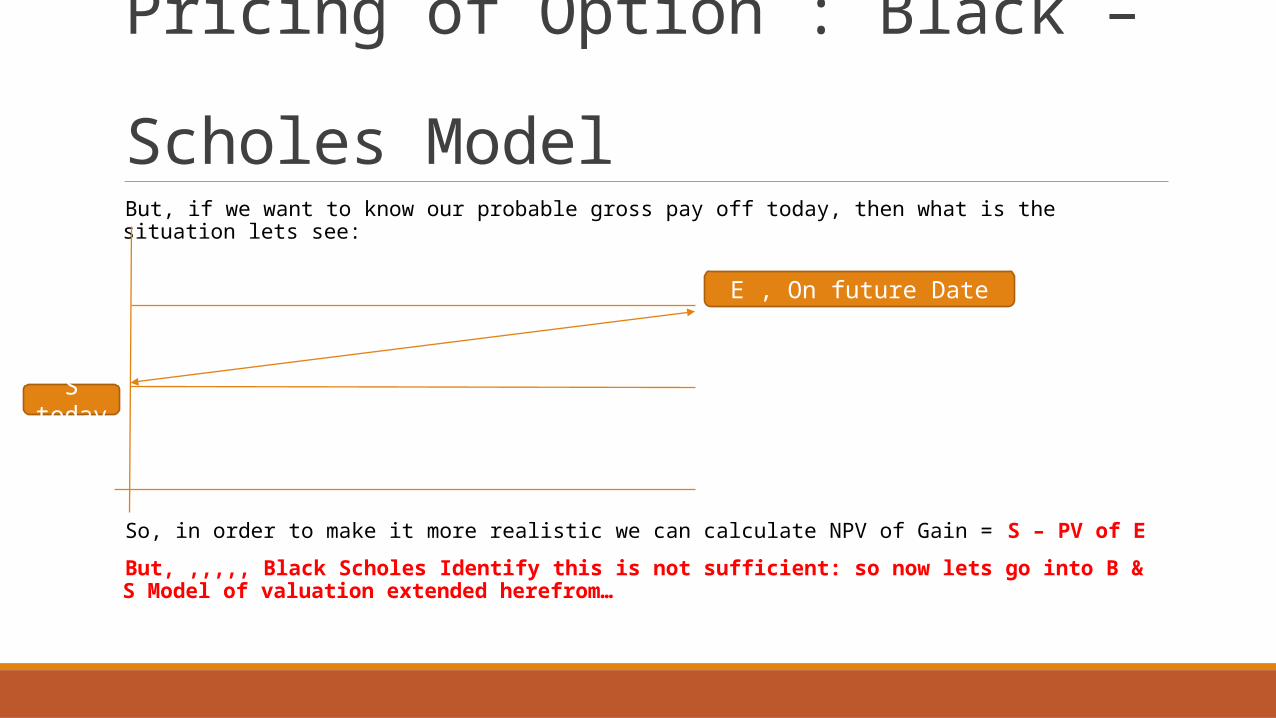
But, if we want to know our probable gross pay off today, then what is the situation lets see:

So, in order to make it more realistic we can calculate NPV of Gain = S – PV of E

But, ,,,,, Black Scholes Identify this is not sufficient: so now lets go into B & S Model of valuation extended herefrom…

E , On future Date

S today


The Black-Scholes formula is an expression for the current value of a European call option on a stock which pays no dividends before expiration of the option.

The formula expresses the call value as the current stock price times a probability factor N(d1), minus the discounted exercise payment times a second probability factor N(d2).

Value = Current MP x N(d1) – PV of Exercise Price x N(d2)

= So x N(d1) – (E x e-rt ) x N(d2)

Here,d = standardized normal random variable &N(d) = Cumulative standardized normal probability distribution.


Initial to Black Scholes Model, two model of valuation of Option came in existence:

A. Risk Neutral Model: assumed that option with one year life, price changes in stock happens only once a year

B. Binomial Model: It is an advancement of Risk Neutral Model. It kept the life of option as similar ONE YEAR but Assumed That Price Change TWICE ( every 6 mth).

BUT, We know that the price of the stock are volatile and keeps changing continuously.

So considering the said fact, there came an existence of new Model, DRAFTED Out by FISHER BLACK & MYRON SCHOLES named as Black Scholes Model.

Value = Current MP x N(d1) – PV of Exercise Price x N(d2) = So x N(d1) – (E x e-rt ) x N(d2)


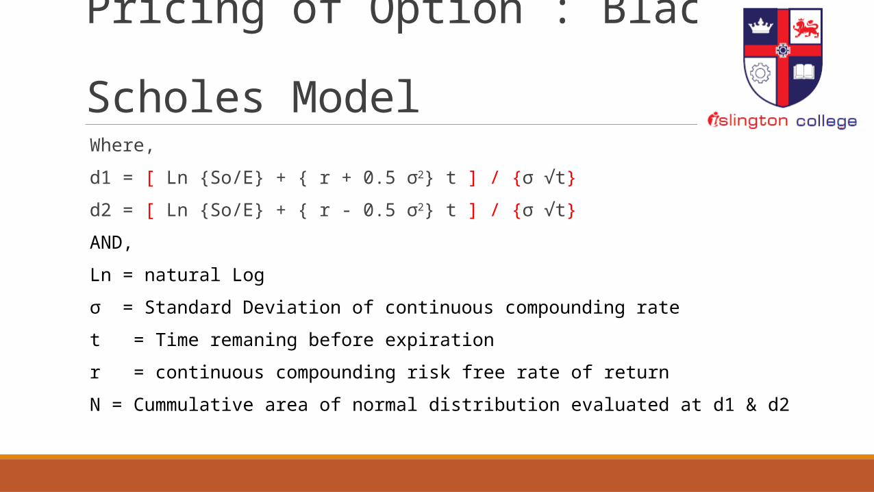
Where,

d1 = [ Ln {So/E} + { r + 0.5 σ2} t ] / {σ √t}

d2 = [ Ln {So/E} + { r - 0.5 σ2} t ] / {σ √t}

AND,

Ln = natural Log

σ = Standard Deviation of continuous compounding rate

t = Time remaning before expiration

r = continuous compounding risk free rate of return

N = Cummulative area of normal distribution evaluated at d1 & d2

Understanding N(d1) & N(d2)

However no more explanation were found in the research paper of B & S regarding this N(d1) &

N(d2).

As the valuation principle is only for In the money call, so we might have some probability that

the option may by ITM or ATM/OTM.

we know PV of E = E x e ^ rt.

But, are we sure that this is going to happen. I.e. the call is going to be exercised in future?

The answer comes, NO….. It might be exercised or it might not be.

So what is the probability that it might be exercised??

The answer is N(d2)….

Therefore N(d2) reflects the risk adjusted probability that the option will be exercised.


N(d1) is the factor by which the present value of contingent receipt of the stock

exceeds the current stock price.


We know:

Pay Off = St - E,

Where , St = Value of Stock at expiration & E = exercise price.

Now, if we want to derive the pay off right now at current date then in simple term we may

calculate the PV of each component (i.e. St & E) and say that the pay off at todays date is NPV of

pay off at time “t”.

BUT, aren’t we missing some thing?


WHAT?

Q1. Is it sure that the option tomorrow will be In the Money? As if the option tomorrow will not

end as ITM than there is no worth of doing all these as we wont be exercising the option in

future.

Q2. While calculating PV of St, how are we going to calculate the same? As we don’t know St

today.

So,,, How are we going to move?


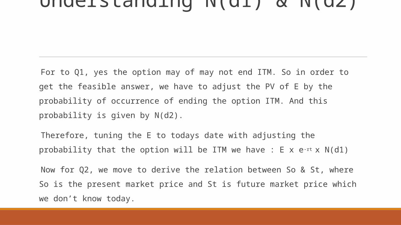
For to Q1, yes the option may of may not end ITM. So in order to get the feasible answer, we

have to adjust the PV of E by the probability of occurrence of ending the option ITM. And this

probability is given by N(d2).

Therefore, tuning the E to todays date with adjusting the probability that the option will be ITM

we have : E x e-rt x N(d1)

Now for Q2, we move to derive the relation between So & St, where So is the present market

price and St is future market price which we don’t know today.

We know, if we have a Rs So today, we can invest the same in risk free investment and get Sf in time t. where Sf is the FV of risk free investment.

OR, Buy a stock at So and let it convert to St in time t.

Here, at the expiration of time “t”, return we get in two situation may or may not be similar.

Lets see how “So” gets converted into “Sf” and “St”

Sf = So ( 1 + r ) ^ n

St = So ( 1 + r ) ^ n X Risk Factor

This risk factor denotes return rate which we get by taking the risk.

Now we get, a relation between St & So , didn’t we. St = So x “FVF” x Risk Factor

Or, St/ FVF = So x Risk Factor

Or, St x e-rt = So x Risk Factor

Now this risk factor is denoted as N(d1), and relates to the factor by which the present value of contingent receipt of the stock exceeds the current stock price.

St x e-rt = So x N(d1)

Example: Consider the following for call option Current Share Price : Rs 120 Exercise Price : Rs 115 Time period : 3 mth Stand Deviation of CCRFI : 0.6 CCRFI : 10% Compute the value of Call using Black Scholes

Call Price = S x N(d1) – (E x e ^-rt x N(d2)Terms Calculation Results

S Given 120

E Given 115

PV of E E x e ^-rt = 115 x e^(-0.10*0.25) = 115 x 0.97533 112.16

Log(S/E) Log(120/115) 0.03922

d1 [ Ln {So/E} + { r + 0.5 σ2} t ] / {σ √t} = { 0.03922 + (0.1+0.18)*0.25} / 0.3

0.3641

d2 d2 = [ Ln {So/E} + { r - 0.5 σ2} t ] / {σ √t} 0.064

N(d1) D1 is positive hence thevalue will fall on Rt hand side.Table value for 0.3641 = 0.1406Cummulative value = 0.5 + table value = 0.5 +0.1406

0.6406

N(d2) Cummulative Value = 0.5 + table value = 0.5 +0.0239 0.5239

Call value (120 x 0.6406) – (112.16 x 0.5239) 18.112

BEST REGARDS

Documents

Introduction to Financial Engineering Aashish Dhakal Week 5: Black Scholes Model