Embed Size (px)
Citation preview

Introduction to Electricity
Network Modelling
Daniel Huppmann & Friedrich Kunz
PhD Winterschool, Oppdal March 2011
- 2 -
Agenda
1. Introduction to Electricity Markets
2. The Electricity Market Model (ELMOD)
3. Congestion Management
4. Exercise: 3-Node Network
5. Introducing Wind Power
6. Exercise: Stochastic Multi-Period European Network
7. Outlook and further developments
Literature

- 3 -
• Non storable
• Grid-bound
• High fix cost ratio
• Economies of scale in generation and transmission
• Daily and seasonal demand patterns
• Power flows according to physical laws (Kirchhoff)
Value added chain
1. Generation
2. Transmission/Distribution
3. Supply
Electricity
- 4 -
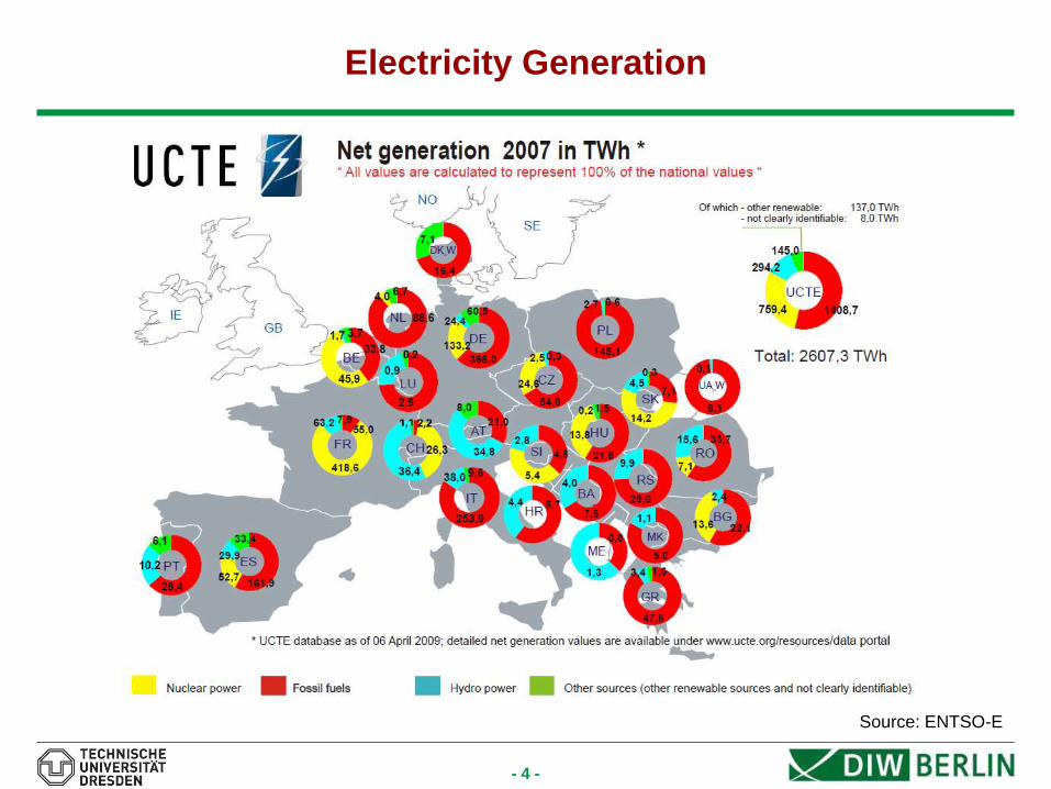
Electricity Generation
Source: ENTSO-E
- 5 -
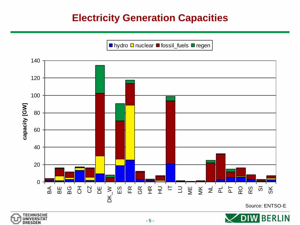
Electricity Generation Capacities
0
20
40
60
80
100
120
140
BA
BE
BG
CH
CZ
DE
DK
_W ES
FR
GR
HR
HU IT LU
ME
MK
NL
PL
PT
RO
RS SI
SK
cap
acit
y [
GW
]
hydro nuclear fossil_fuels regen
Source: ENTSO-E

- 6 -
77,886,2
7,9
6,4
23,8
0
20
40
60
80
100
120
140
Planttype Power Banlance Peak Load
Po
wer
[GW
]Plant Capacity and Peak Load in Germany 2006
Hydro
Lignite
Nuclear
Coal
Gas
Oil
PSP.
Renewable thereof
has to be covered
non available capacity
outages and revision
reserve capacities
available capacity
Source: VDN 2006
At time of peak load an export surplus of 2.1GW occured
Sufficient capacity to supply Germany and still export:

- 7 -
The Merit-Order Cost Curve and
Pricing under Competition
Quantity
[MWh]
Price
[€/MWh]
Demand
Competiton
Competiton
Merit Order
- 8 -
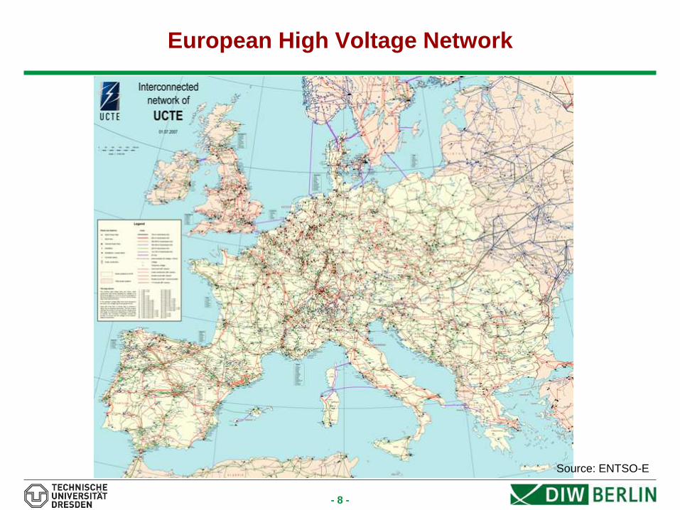
European High Voltage Network
Source: ENTSO-E
- 9 -
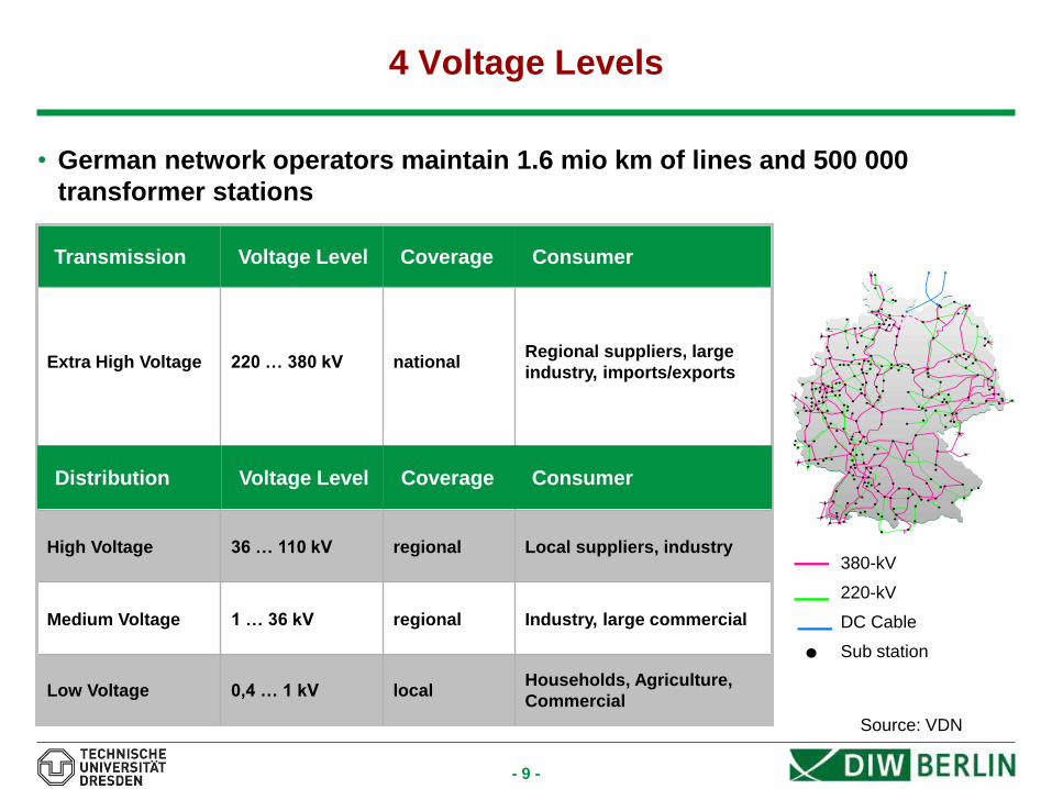
4 Voltage Levels
• German network operators maintain 1.6 mio km of lines and 500 000
transformer stations
Source: VDN
380-kV
220-kV
DC Cable
Sub station
local
regional
regional
national
•Coverage
Households, Agriculture,
Commercial 0,4 … 1 kV Low Voltage
Industry, large commercial 1 … 36 kV Medium Voltage
Local suppliers, industry 36 … 110 kV High Voltage
Regional suppliers, large
industry, imports/exports 220 … 380 kV Extra High Voltage
•Consumer •Voltage Level •Transmission
•Coverage •Consumer •Voltage Level •Distribution
- 10 -
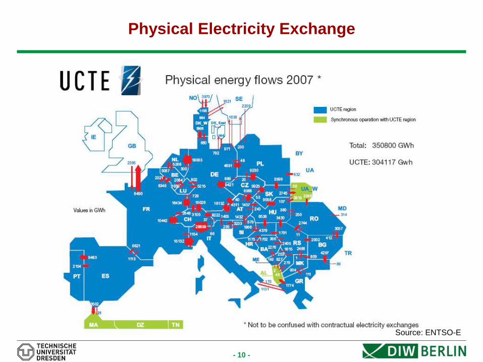
Physical Electricity Exchange
Source: ENTSO-E
- 11 -
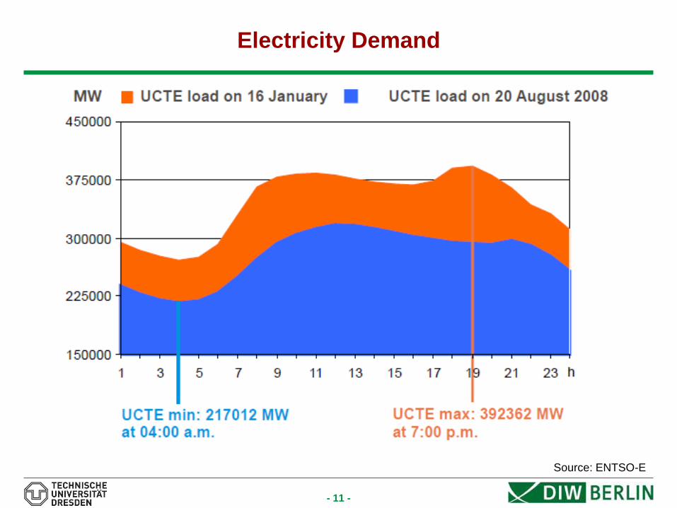
Electricity Demand
Source: ENTSO-E

- 12 -
Agenda
1. Introduction to Electricity Markets
2. The Electricity Market Model (ELMOD)
3. Congestion Management
4. Exercise: 3-Node Network
5. Introducing Wind Power
6. Exercise: Stochastic Multi-Period European Network
7. Outlook and further developments
Literature
- 13 -
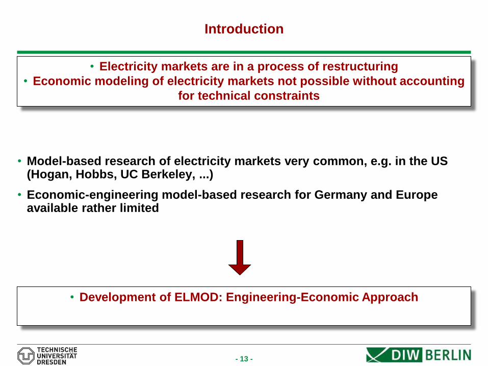
Introduction
• Model-based research of electricity markets very common, e.g. in the US (Hogan, Hobbs, UC Berkeley, ...)
• Economic-engineering model-based research for Germany and Europe available rather limited
• Electricity markets are in a process of restructuring
• Economic modeling of electricity markets not possible without accounting
for technical constraints
• Development of ELMOD: Engineering-Economic Approach
- 14 -
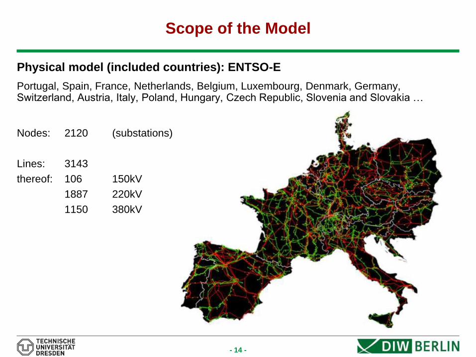
Scope of the Model
Physical model (included countries): ENTSO-E
Portugal, Spain, France, Netherlands, Belgium, Luxembourg, Denmark, Germany, Switzerland, Austria, Italy, Poland, Hungary, Czech Republic, Slovenia and Slovakia …
Nodes: 2120 (substations)
Lines: 3143
thereof: 106 150kV
1887 220kV
1150 380kV
- 15 -
Market Assumptions and Data
• Market: - No strategic players Perfect competition
- Perfect market bidding (marginal cost bids, no market power)
- Independent SO optimizes generation dispatch and network usage simultaneously
• Node demand: - Linear inverse demand function constructed using
- a reference demand,
- a reference price, and
- a point demand elasticity
- Reference demands are based on ENTSO-E data and distributed to system nodes
according to regional population and/or gross domestic product
- Reference prices are based on the spot prices of the national energy exchange
• Wind input: - Given as external parameter based on wind distributions derived from historic data
• Reference: Leuthold et al. (2010)
- 16 -
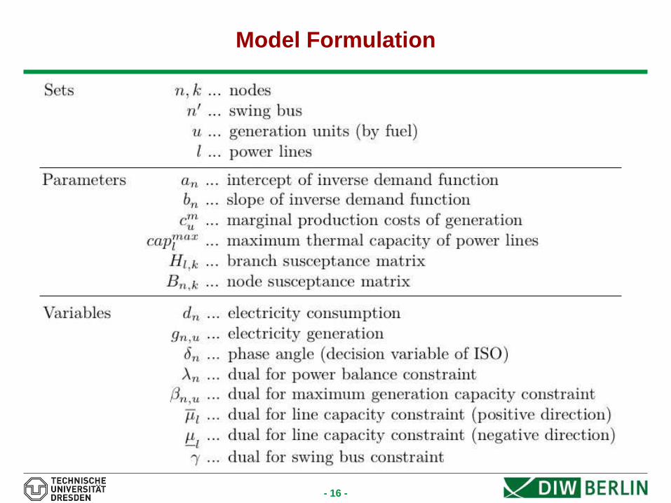
Model Formulation

- 17 -
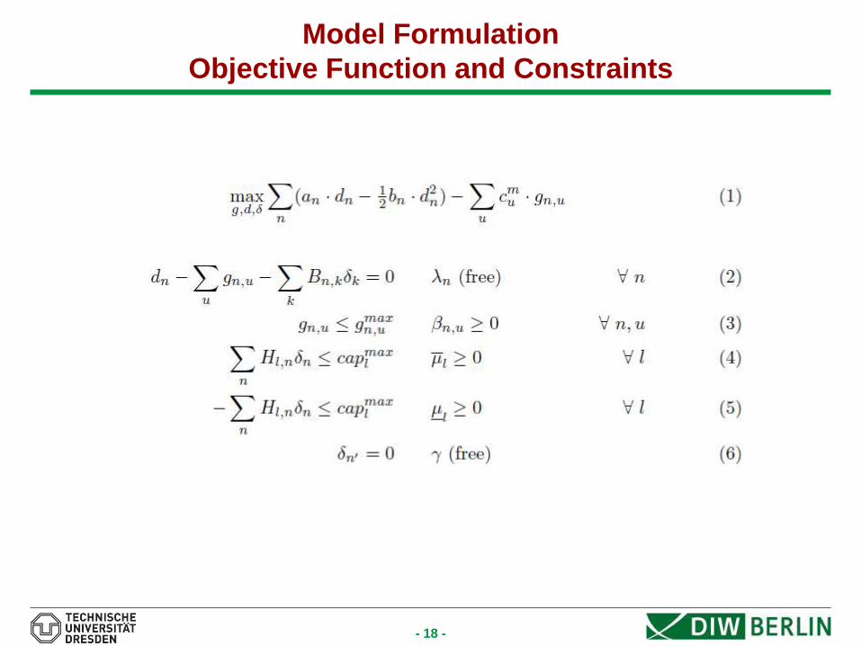
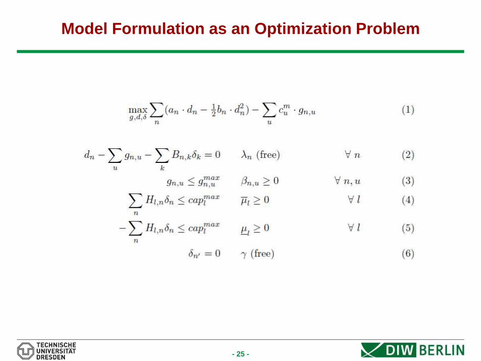
Model Formulation
Objective Function and Constraints
Given: generation capacities, network, demand function, wind
Decide about: generation, demand
max (Social Welfare)
subject to:
demand = generation + netinput
generation <= installed capacity
ABS(loadflow) <= thermal limit
- 18 -
Model Formulation
Objective Function and Constraints
- 19 -
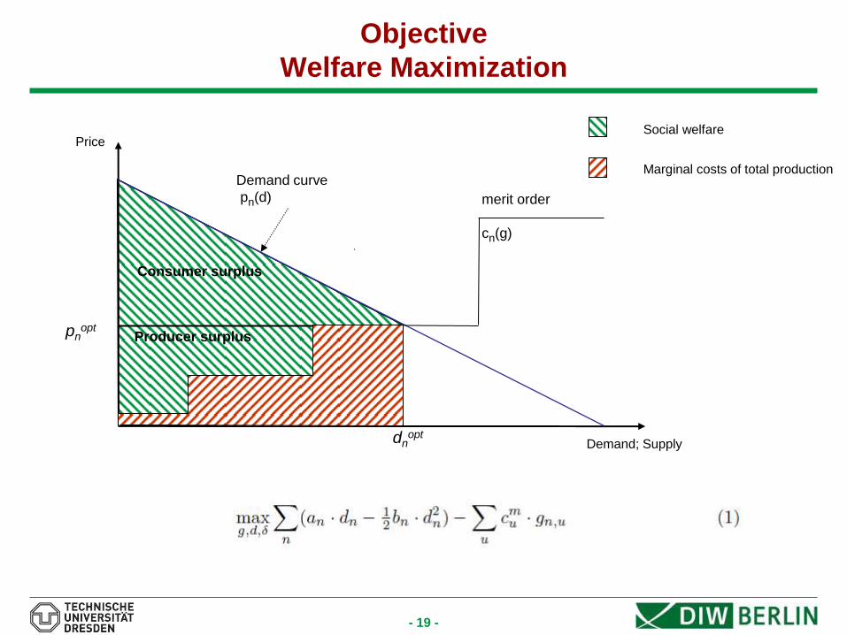
Objective
Welfare Maximization
Price
Demand; Supply
merit order
cn(g)
Marginal costs of total production
Social welfare
Demand curve
pn(d)
Consumer surplus
Producer surplus pnopt
dnopt

- 20 -
Market Clearing Constraint
or Nodal Energy Balance
• Main characteristics of electricity
- Non storable
- Grid-bounded
Supply has to be equal to demand
Exchange between system nodes through transmission network
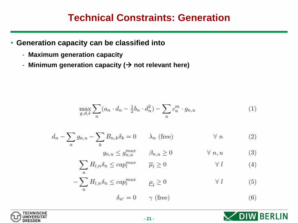
- 21 -
Technical Constraints: Generation
• Generation capacity can be classified into
- Maximum generation capacity
- Minimum generation capacity ( not relevant here)
- 22 -
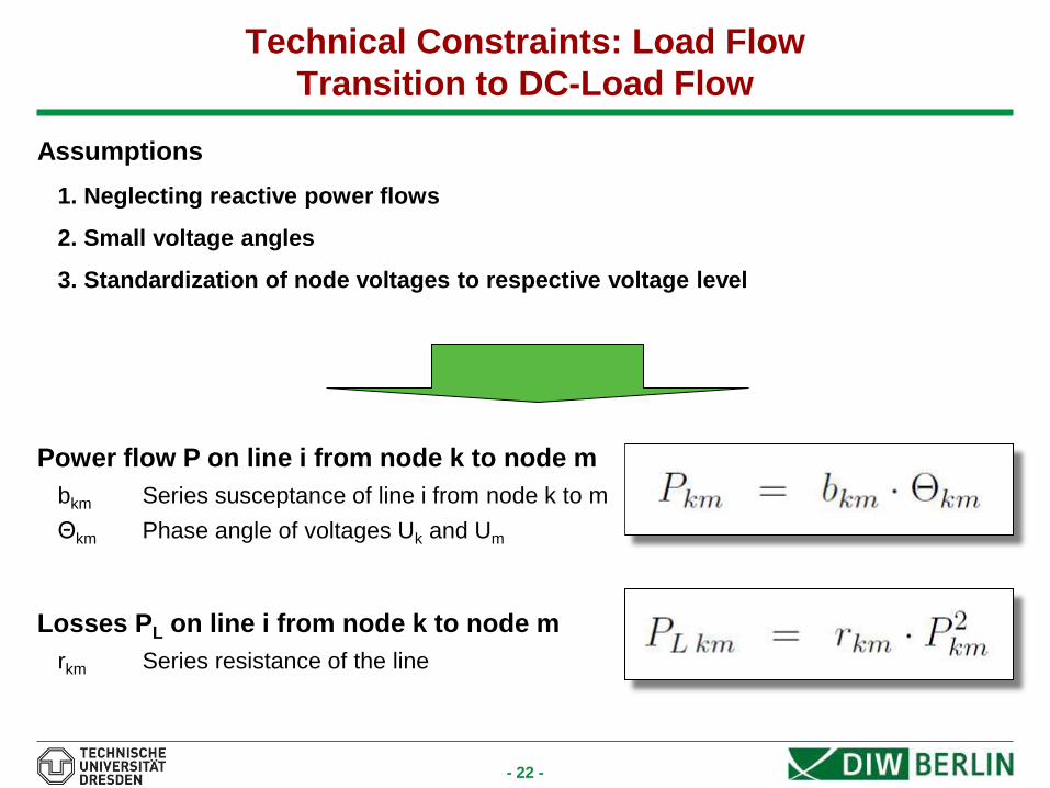
Technical Constraints: Load Flow
Transition to DC-Load Flow
Assumptions
1. Neglecting reactive power flows
2. Small voltage angles
3. Standardization of node voltages to respective voltage level
Power flow P on line i from node k to node m
bkm Series susceptance of line i from node k to m
Θkm Phase angle of voltages Uk and Um
Losses PL on line i from node k to node m
rkm Series resistance of the line

- 23 -
Technical Constraints: Load Flow
Summary
- 24 -
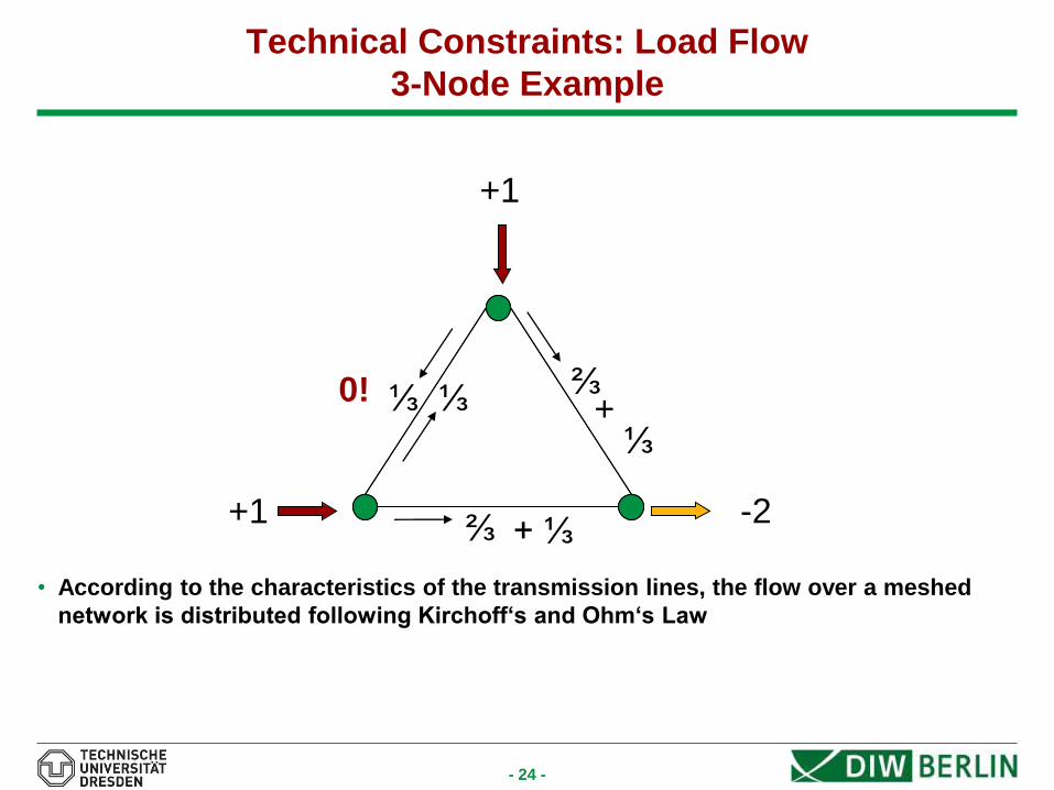
Technical Constraints: Load Flow
3-Node Example
⅓
⅔ +1
• According to the characteristics of the transmission lines, the flow over a meshed
network is distributed following Kirchoff‘s and Ohm‘s Law
⅓ ⅔
+1
+ ⅓
+ ⅓
0!
-2
- 25 -
Model Formulation as an Optimization Problem
- 26 -
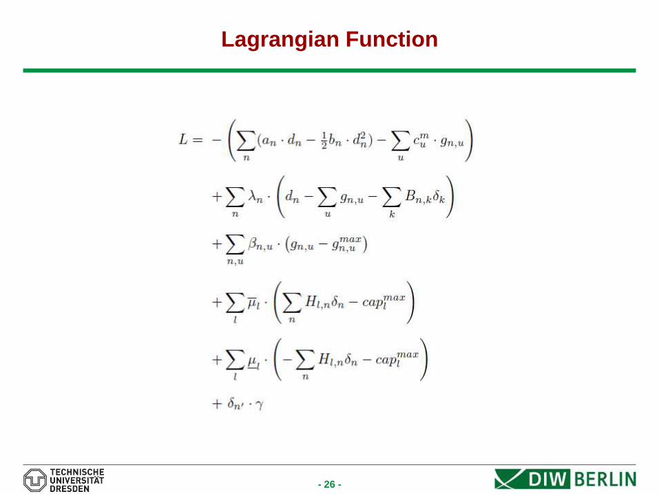
Lagrangian Function

- 27 -
Karush-Kuhn-Tucker Conditions

- 28 -
Agenda
1. Introduction to Electricity Markets
2. The Electricity Market Model (ELMOD)
3. Congestion Management
4. Exercise: 3-Node Network
5. Introducing Wind Power
6. Exercise: Stochastic Multi-Period European Network
7. Outlook and further developments
Literature
- 29 -
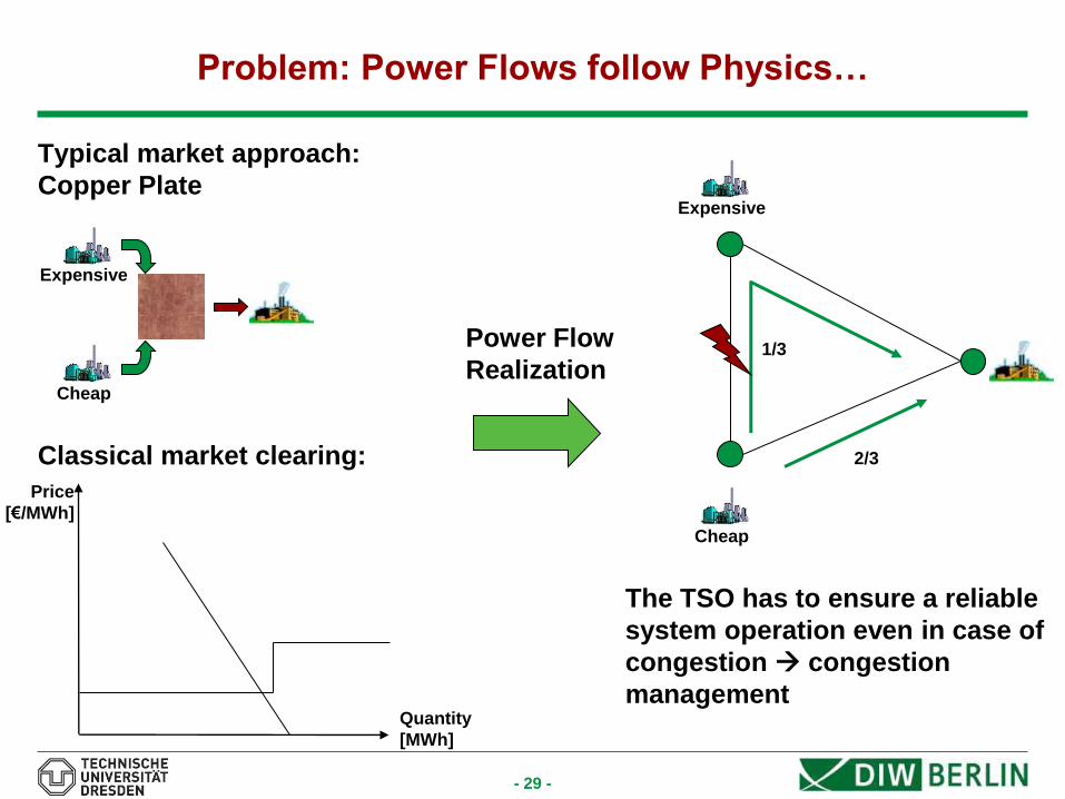
Problem: Power Flows follow Physics…
Typical market approach:
Copper Plate
Classical market clearing:
Quantity
[MWh]
Price
[€/MWh]
Cheap
Expensive
Power Flow
Realization
Cheap
Expensive
2/3
1/3
The TSO has to ensure a reliable
system operation even in case of
congestion congestion
management

- 30 -
The Theory of Nodal Pricing
• Nodal Pricing (often also referred to as Locational Marginal Pricing (LMP)):
- there is a separate price for energy for each node in the network
- containing cost of generation, losses and transmission (“implicit auction“)
• Nodal Prices result from the cost:
- for the supply of an additional MW(h) energy
- at a specific node in the grid
- while using the available least-cost generation unit(s)
- subject to network constraints
Nodal Price Marginal Cost
of Generation
Cost of
Congestion
Cost of
Marginal
Losses = + +

- 31 -
Impact on Objective Function
Price
Demand; Supply
merit order
cn(g)
Marginal costs of total production
Social welfare
Demand curve
pn(d)
Consumer surplus
Producer surplus
pncong
pnopt
dncong dn
opt
pncong In the case of congestion the nodal
price deviates from the optimum
- 32 -
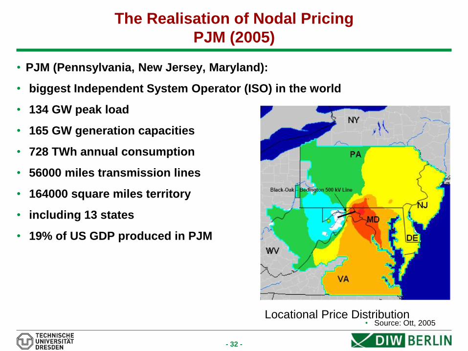
The Realisation of Nodal Pricing
PJM (2005)
• PJM (Pennsylvania, New Jersey, Maryland):
• biggest Independent System Operator (ISO) in the world
• 134 GW peak load
• 165 GW generation capacities
• 728 TWh annual consumption
• 56000 miles transmission lines
• 164000 square miles territory
• including 13 states
• 19% of US GDP produced in PJM
Locational Price Distribution • Source: Ott, 2005

- 33 -
Nodal vs Zonal Pricing
• Nodal Pricing not applied in Europe
• European countries use zonal pricing
- Price zones fixed and equal to country (e.g. Germany, Belgium, France)
- Price zones fixed, but several zones within a country (e.g. Italy, Norway)
- Price zones flexible according to network congestion Nodal Pricing
• Implementation of zonal pricing in ELMOD
- Additional restriction which ensures equality of prices with a price zone
- a(n) + b(n)*q(n) =e= p(z) forall nodes n in zone z

- 34 -
Agenda
1. Introduction to Electricity Markets
2. The Electricity Market Model (ELMOD)
3. Congestion Management
4. Exercise: 3-Node Network
5. Introducing Wind Power
6. Exercise: Stochastic Multi-Period European Network
7. Outlook and further developments
Literature
- 35 -
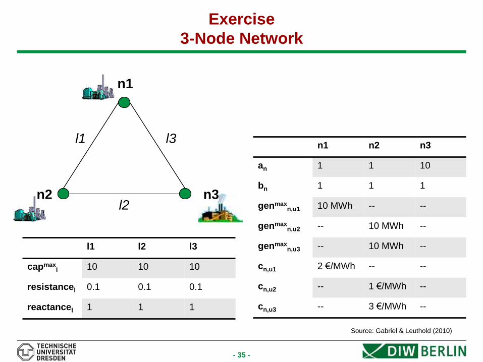
Exercise
3-Node Network
l2 n3
n1
l1 l3
n2
Source: Gabriel & Leuthold (2010)
n1 n2 n3
an 1 1 10
bn 1 1 1
genmaxn,u1 10 MWh -- --
genmaxn,u2 -- 10 MWh --
genmaxn,u3 -- 10 MWh --
cn,u1 2 €/MWh -- --
cn,u2 -- 1 €/MWh --
cn,u3 -- 3 €/MWh --
l1 l2 l3
capmaxl 10 10 10
resistancel 0.1 0.1 0.1
reactancel 1 1 1

- 36 -
Exercise
3-Node Network
OPEN GAMS
OPEN OWS_3N_elmod.gms
- 37 -
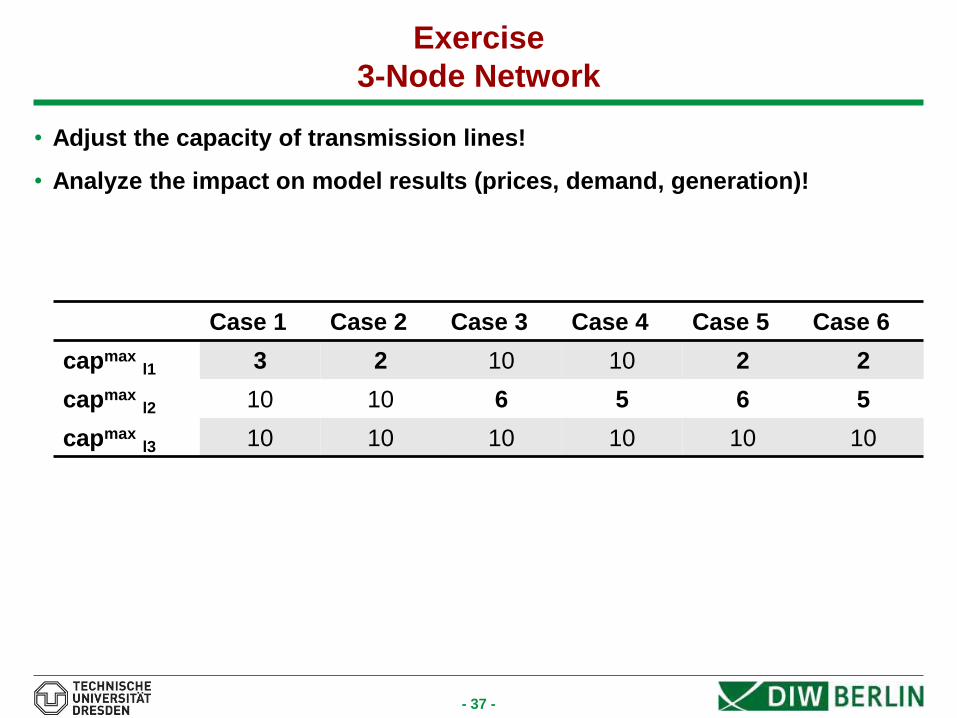
Exercise
3-Node Network
• Adjust the capacity of transmission lines!
• Analyze the impact on model results (prices, demand, generation)!
Case 1 Case 2 Case 3 Case 4 Case 5 Case 6
capmax l1 3 2 10 10 2 2
capmax l2 10 10 6 5 6 5
capmax l3 10 10 10 10 10 10
- 38 -
Exercise
3-Node Network
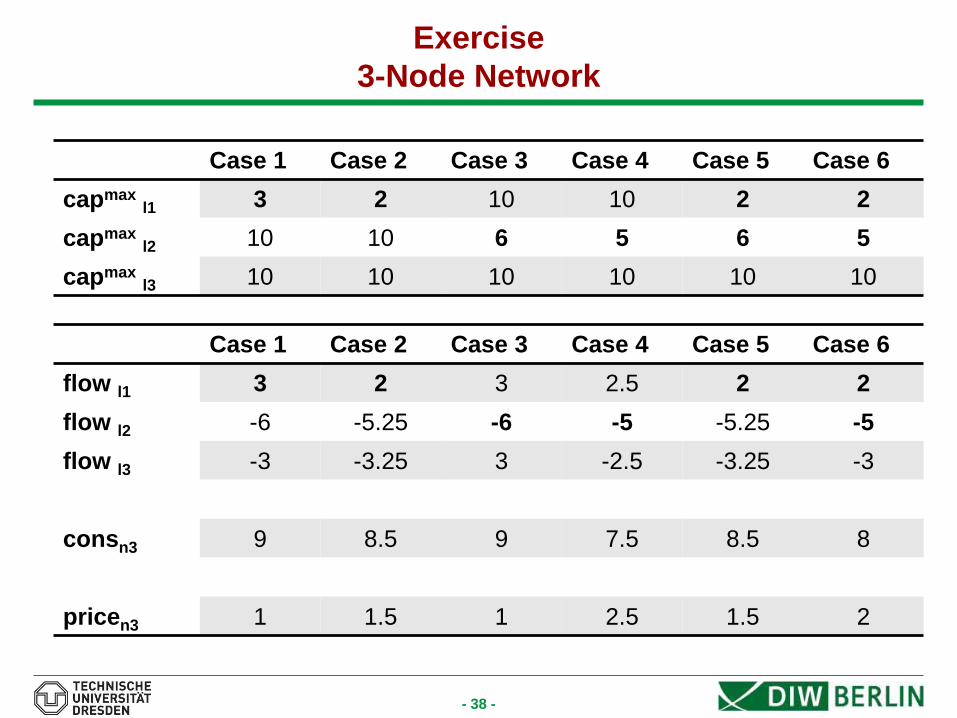
Case 1 Case 2 Case 3 Case 4 Case 5 Case 6
capmax l1 3 2 10 10 2 2
capmax l2 10 10 6 5 6 5
capmax l3 10 10 10 10 10 10
Case 1 Case 2 Case 3 Case 4 Case 5 Case 6
flow l1 3 2 3 2.5 2 2
flow l2 -6 -5.25 -6 -5 -5.25 -5
flow l3 -3 -3.25 3 -2.5 -3.25 -3
consn3 9 8.5 9 7.5 8.5 8
pricen3 1 1.5 1 2.5 1.5 2
- 39 -
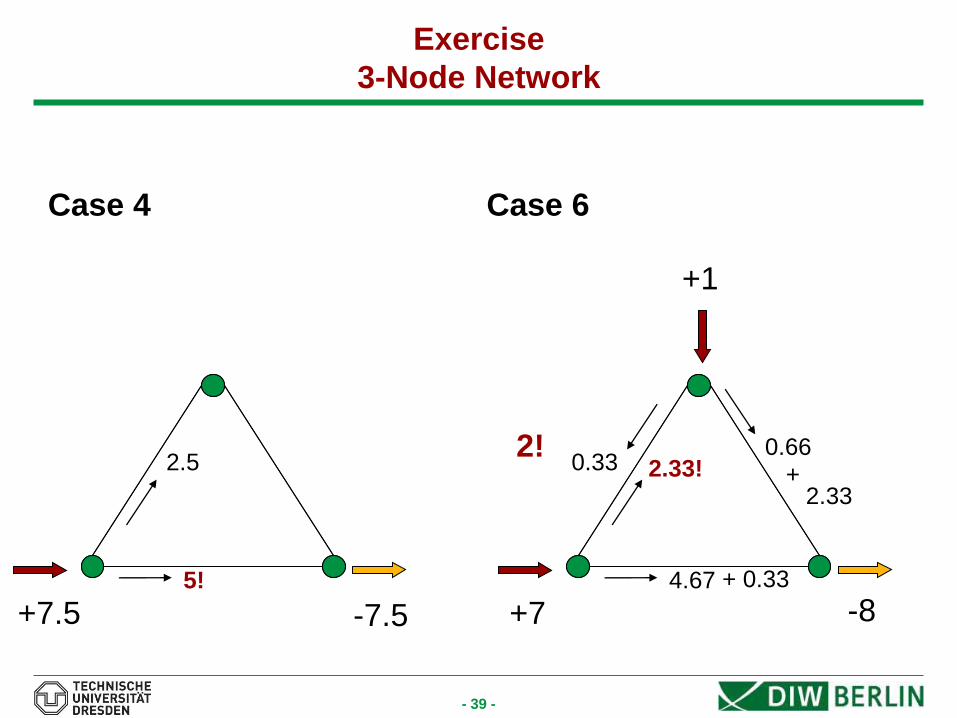
Exercise
3-Node Network
Case 4 Case 6
2.5
5!
+7.5 -7.5
2.33!
4.67
+7
0.33 0.66
+1
+ 0.33
+ 2.33
2!
-8

- 40 -
Agenda
1. Introduction to Electricity Markets
2. The Electricity Market Model (ELMOD)
3. Congestion Management
4. Exercise: 3-Node Network
5. Introducing Wind Power
6. Exercise: Stochastic Multi-Period European Network
7. Outlook and further developments
Literature

- 41 -
Wind mills in medieval times
14th century windmill; http://en.wikipedia.org/wiki/History_of_wind_power

- 42 -
Charles F. Brush's windmill (built in 1887)
12kW, 17 meter diameter rotor; http://en.wikipedia.org/wiki/History_of_wind_power
- 43 -
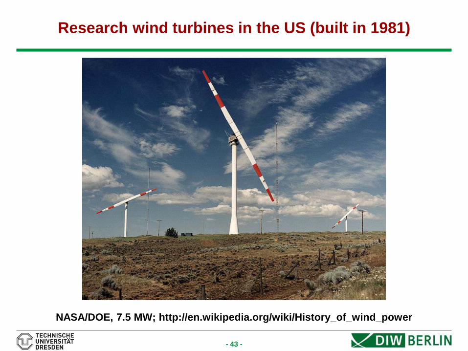
Research wind turbines in the US (built in 1981)
NASA/DOE, 7.5 MW; http://en.wikipedia.org/wiki/History_of_wind_power

- 44 -
Probability distribution of wind speed
Weibull distribution (two parameters)
- Probability distribution function
x...wind speed
β...shape parameter
η...scale parameter
- Cumulative distribution function
- Mean
• The Weibull distribution is commonly used for wind speed probability
using a shape parameter β = 2 for Europe and North America
Probability distribution function
β = 2, η = 8
f (x)
x
1
exp x
, x 0
F(x) 1 exp x
, x 0
mean 1
1
- 45 -
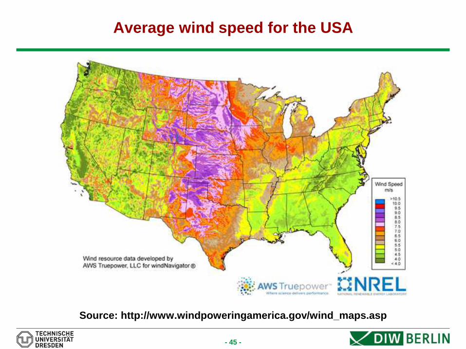
Average wind speed for the USA
Source: http://www.windpoweringamerica.gov/wind_maps.asp

- 46 -
Power of wind
• Newtons second law of motion:
P...power of wind
ρ...density of dry air
x...wind speed
r...radius of the rotor
• Betz law:
Formulated by German physicist Albert Betz in 1919
Published „Wind-Energie“ in 1926
„you can only convert less than 16/27 (or 59%) of the
kinetic energy in the wind to mechanical energy
using a wind turbine“
Danish Wind Industry Association – http://guidedtour.windpower.org/
P 1
2x3r2
- 47 -
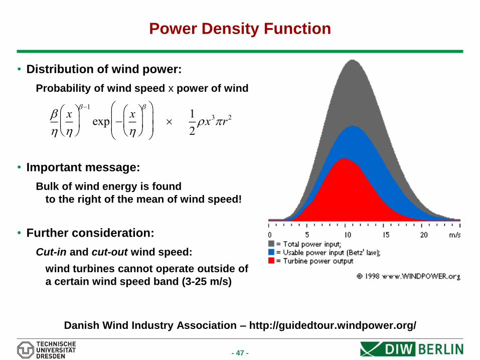
Power Density Function
• Distribution of wind power:
Probability of wind speed x power of wind
• Important message:
Bulk of wind energy is found
to the right of the mean of wind speed!
• Further consideration:
Cut-in and cut-out wind speed:
wind turbines cannot operate outside of
a certain wind speed band (3-25 m/s)
Danish Wind Industry Association – http://guidedtour.windpower.org/
x
1
exp x
1
2x3r2

- 48 -
Some References on Electricity Data, Wind, etc.
• References for Electricity Data
- European Network of Transmission System Operators for Electricity
- https://www.entsoe.eu/resources/data-portal/
- EUROSTAT
- http://epp.eurostat.ec.europa.eu/portal/page/portal/eurostat/home/
• References for Wind Power Generation
- Danish Wind Industry Association
- http://guidedtour.windpower.org
- http://www.talentfactory.dk/
- US Department of Energy
- http://www.windpoweringamerica.gov/
- http://www.eere.energy.gov/

- 49 -
Agenda
1. Introduction to Electricity Markets
2. The Electricity Market Model (ELMOD)
3. Congestion Management
4. Exercise: 3-Node Network
5. Introducing Wind Power
6. Exercise: Stochastic Multi-Period European Network
7. Outlook and further developments
Literature
- 50 -
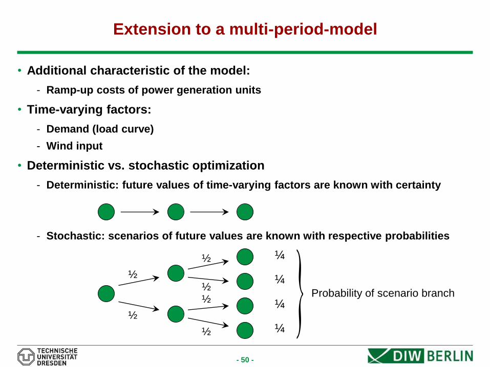
Extension to a multi-period-model
• Additional characteristic of the model:
- Ramp-up costs of power generation units
• Time-varying factors:
- Demand (load curve)
- Wind input
• Deterministic vs. stochastic optimization
- Deterministic: future values of time-varying factors are known with certainty
- Stochastic: scenarios of future values are known with respective probabilities
½
½
½
½ ½
½
¼
¼
¼
¼
Probability of scenario branch }
- 51 -
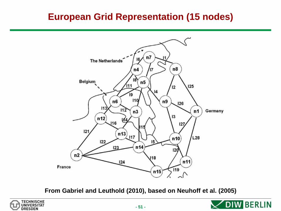
European Grid Representation (15 nodes)
From Gabriel and Leuthold (2010), based on Neuhoff et al. (2005)
- 52 -
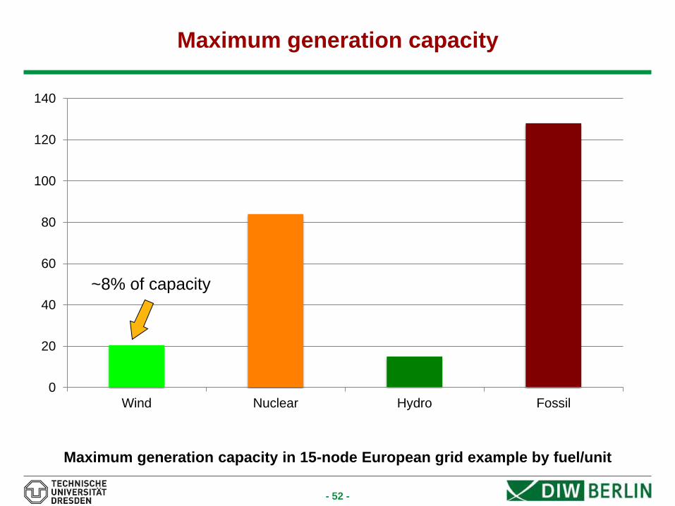
Maximum generation capacity
Maximum generation capacity in 15-node European grid example by fuel/unit
0
20
40
60
80
100
120
140
Wind Nuclear Hydro Fossil
~8% of capacity
- 53 -
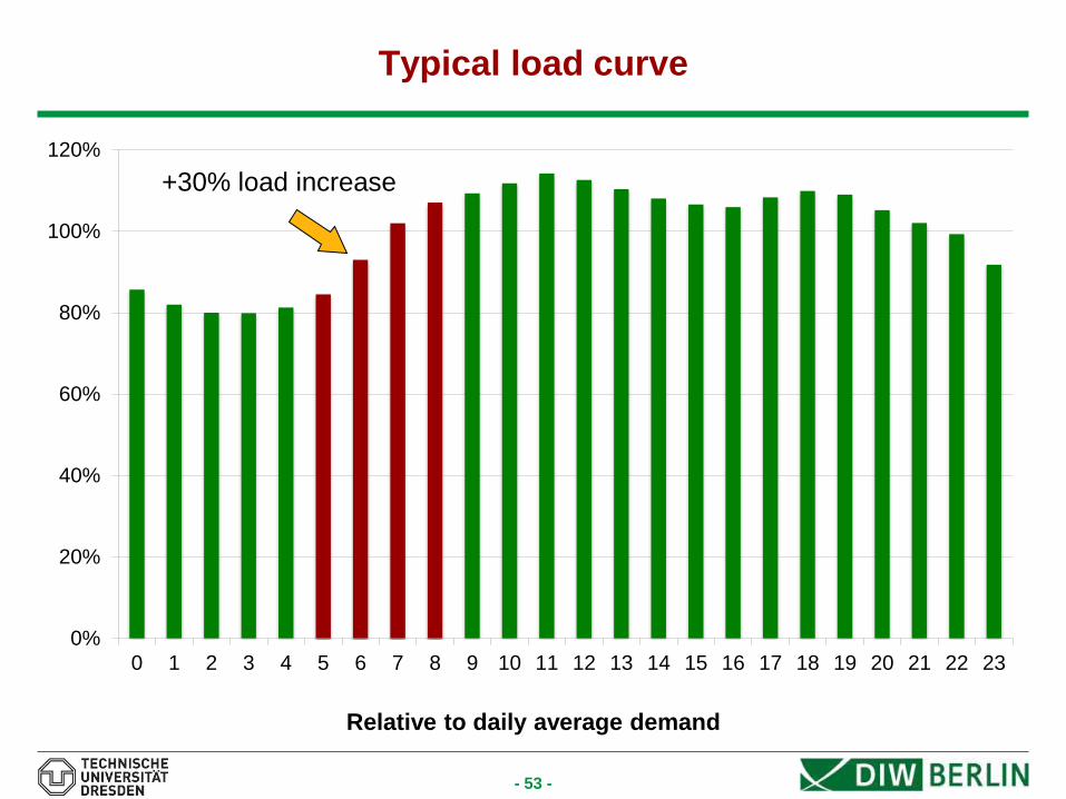
Typical load curve
0%
20%
40%
60%
80%
100%
120%
0 1 2 3 4 5 6 7 8 9 10 11 12 13 14 15 16 17 18 19 20 21 22 23
Relative to daily average demand
+30% load increase
- 54 -
GAMS Exercise: 15 Node European Network
• Focus: time period 5 am – 9 am
- Determine the optimal ramp-up decisions from the point of the ISO
• Assumptions:
- Load curve exogenously given (deterministic)
- Ramp-up at no cost in first period
- Wind power must be fed into the grid
- No wind generation at 5 am
- Wind generation jumps discretely at the full hour
- Wind generation relative to total capacity identical at each node
- 55 -
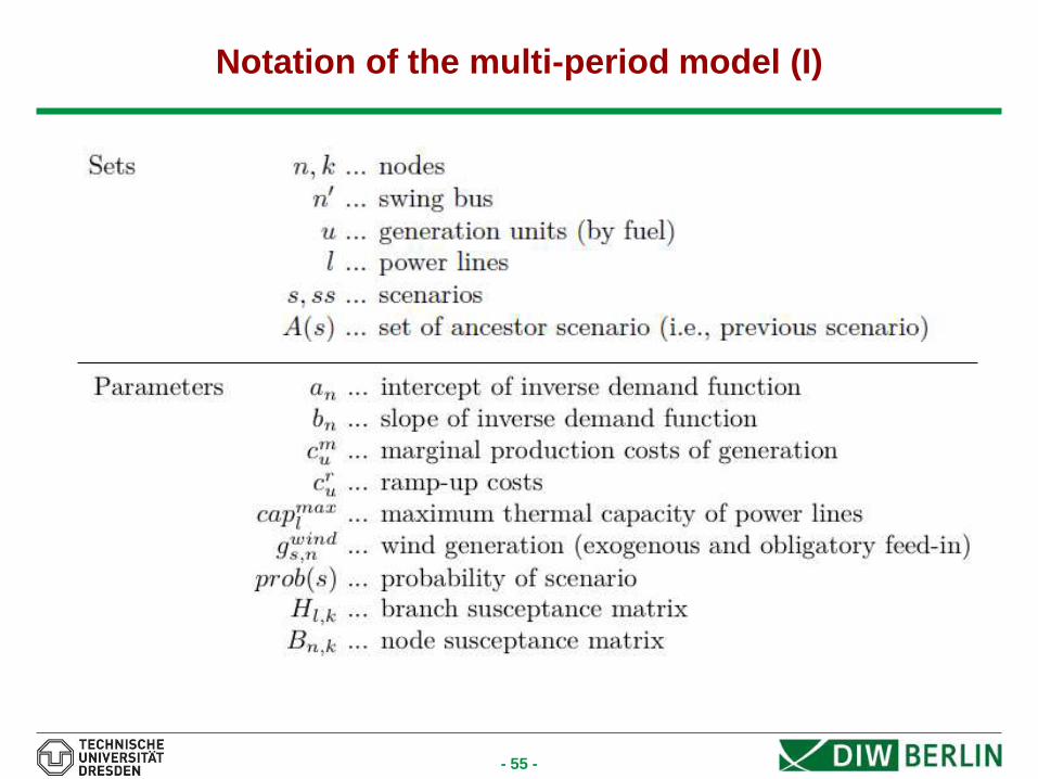
Notation of the multi-period model (I)
- 56 -
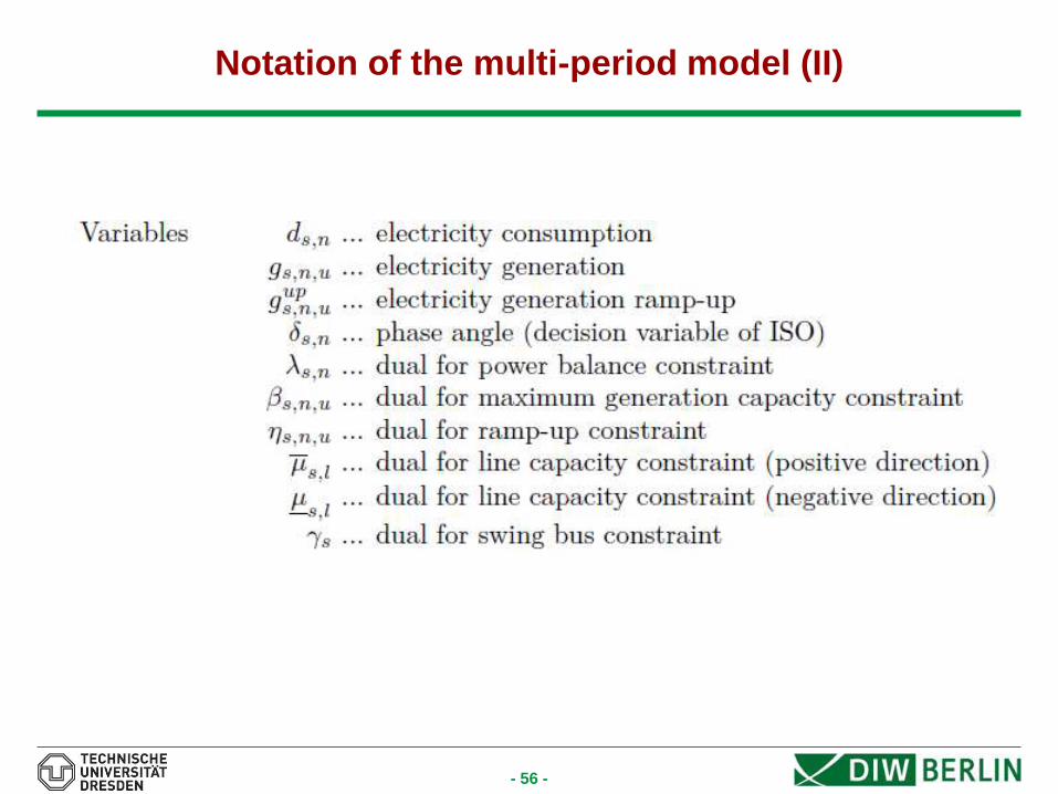
Notation of the multi-period model (II)
- 57 -
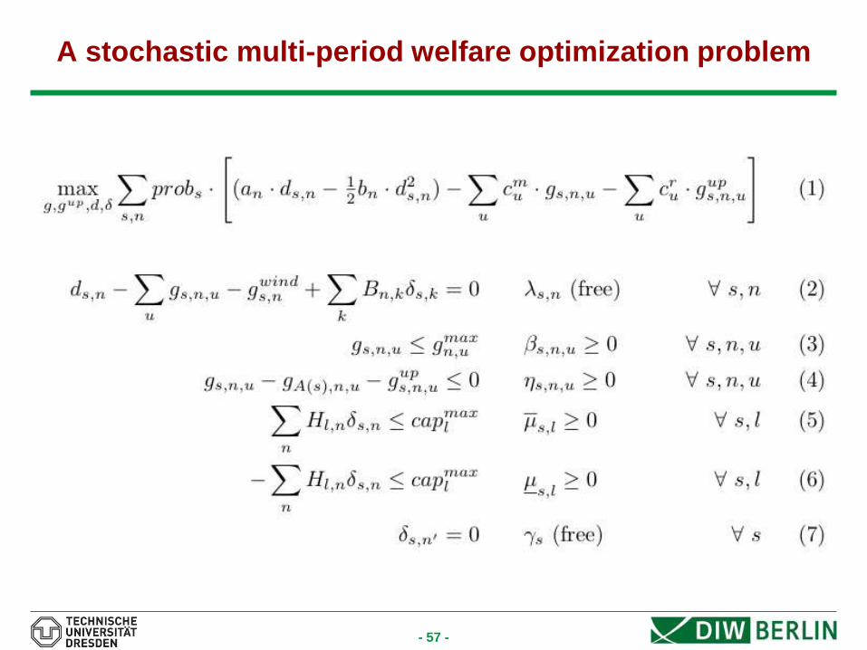
A stochastic multi-period welfare optimization problem
- 58 -
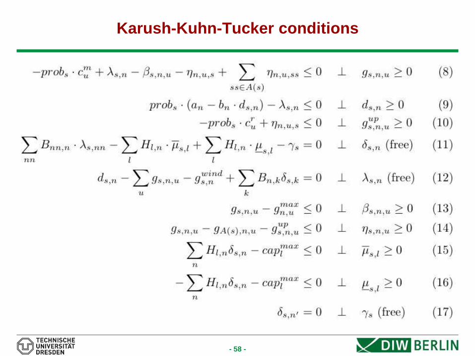
Karush-Kuhn-Tucker conditions

- 59 -
Scenario tree – stochastic wind power generation
Scenario tree and respective wind power relative to maximum capacity
s1
s2
s3
0.25
0
0
s4
s5
0.6
0.2
s6
s7
0.3
0
s8
s9
1.0
0.4
s10
s11
0.8
0.1
s12
s13
0.6
0.2
s14
s15
0.3
0
5 am 6 am 7 am 8 am
- 60 -
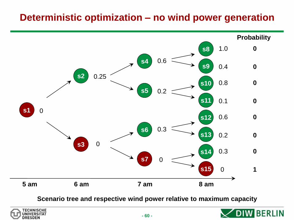
Deterministic optimization – no wind power generation
Scenario tree and respective wind power relative to maximum capacity
s1
s2
s3
0.25
0
0
s4
s5
0.6
0.2
s6
s7
0.3
0
s8
s9
1.0
0.4
s10
s11
0.8
0.1
s12
s13
0.6
0.2
s14
s15
0.3
0
5 am 6 am 7 am 8 am
0
0
0
0
0
0
0
1
Probability
- 61 -
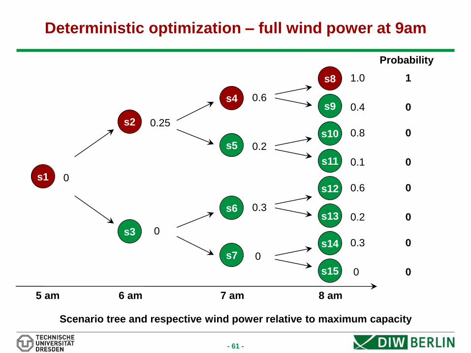
Deterministic optimization – full wind power at 9am
Scenario tree and respective wind power relative to maximum capacity
s1
s2
s3
0.25
0
0
s4
s5
0.6
0.2
s6
s7
0.3
0
s8
s9
1.0
0.4
s10
s11
0.8
0.1
s12
s13
0.6
0.2
s14
s15
0.3
0
5 am 6 am 7 am 8 am
1
0
0
0
0
0
0
0
Probability
- 62 -
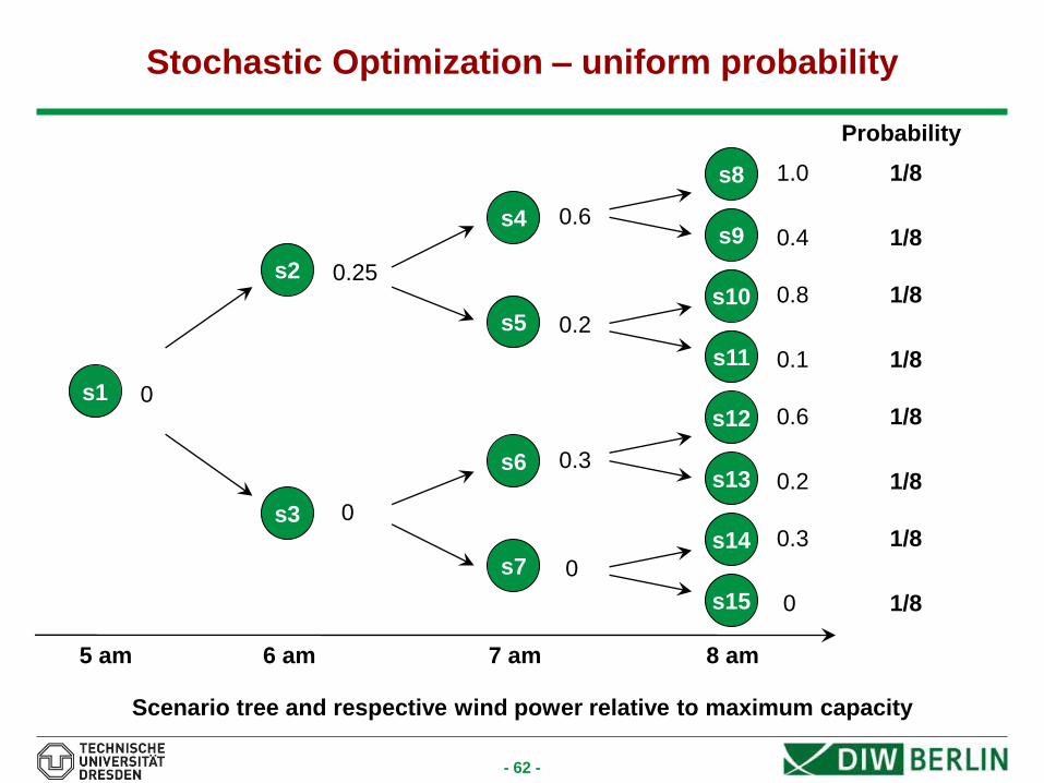
Stochastic Optimization – uniform probability
Scenario tree and respective wind power relative to maximum capacity
s1
s2
s3
0.25
0
0
s4
s5
0.6
0.2
s6
s7
0.3
0
s8
s9
1.0
0.4
s10
s11
0.8
0.1
s12
s13
0.6
0.2
s14
s15
0.3
0
5 am 6 am 7 am 8 am
1/8
1/8
1/8
1/8
1/8
1/8
1/8
1/8
Probability
- 63 -
How to compare scenario simulation results?
• Objective value of optimization problem: welfare
- Difficult to grasp this value intuitively
• Final demand or wholesale prices
- The model is built on locational marginal prices, so there are no „prices“ similar
to the prices observed in the real world
• Dual variables (shadow prices) to the energy balance constraint (λ)
- Which nodes to compare?
- How to weight results from different nodes?
• Consumption-weighted average of energy balance constraint duals
- This is only an index and may hide big variations in welfare/shadow prices
- 64 -
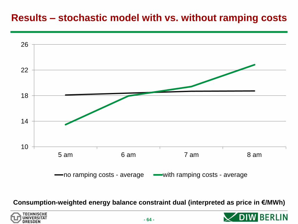
Results – stochastic model with vs. without ramping costs
10
14
18
22
26
5 am 6 am 7 am 8 am
no ramping costs - average with ramping costs - average
Consumption-weighted energy balance constraint dual (interpreted as price in €/MWh)
- 65 -
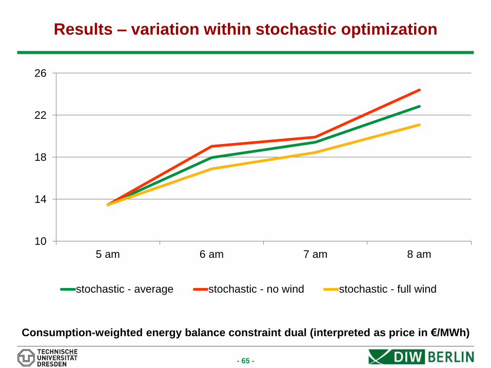
Results – variation within stochastic optimization
10
14
18
22
26
5 am 6 am 7 am 8 am
stochastic - average stochastic - no wind stochastic - full wind
Consumption-weighted energy balance constraint dual (interpreted as price in €/MWh)
- 66 -
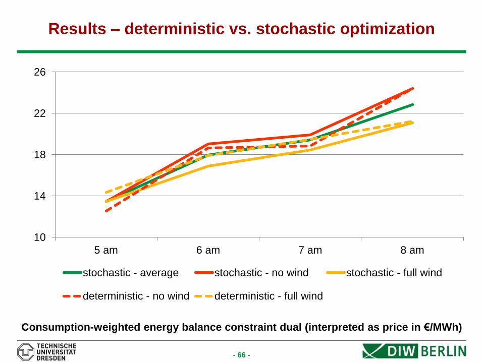
Results – deterministic vs. stochastic optimization
10
14
18
22
26
5 am 6 am 7 am 8 am
stochastic - average stochastic - no wind stochastic - full wind
deterministic - no wind deterministic - full wind
Consumption-weighted energy balance constraint dual (interpreted as price in €/MWh)
- 67 -
Conclusions: stochastic vs. deterministic optimization
• Ramp-up costs lead to lower costs at the beginning of the time horizon, as
power plants are ramped up earlier
- Watch out: there is a bias in this model due to zero ramp-up costs
in the first period by assumption
• This effect is stronger in a deterministic no-wind scenario
• Higher wind input reduces prices (shadow prices to energy balance)
• Uncertainty leads to hedging by the ISO
• Prices converge in last period of deterministic vs. stochastic optimization
- 68 -
Exercise: Stochastic Multi-Period European Network
OPEN GAMS
OPEN OWS_EUR_elmod.gms
- 69 -
Possible Projects
• Nice and easy start
- Variation of ramping-costs
- Variation of probabilities/wind power generation of scenarios
- Analysing the impact of stochasticity on market results (determinisitic vs.
Stochastic model setup, EVPI)
• Investment analysis (policy evaluation)
- Expansion of wind generation capacity
- Investment in new power lines
• Model horizon and data
- Extension of observation period
- Extension of scenario tree
- Norwegian grid representation
• Model developments
- Implementation of endogenous pumped-hydro storage dispatch
- Implementation of zonal pricing

- 70 -
Agenda
1. Introduction to Electricity Markets
2. The Electricity Market Model (ELMOD)
3. Congestion Management
4. Exercise: 3-Node Network
5. Introducing Wind Power
6. Exercise: Stochastic Multi-Period European Network
7. Outlook and further developments
Literature
- 71 -
A better representation of ramping
• In our example, ramping costs are...
- Proportional to the level of ramped-up generation
- Not related to the duration of down-time (i.e., cold-start vs. hot start)
• A more realistic representation would be possible using binary variables
- Introduce a variable to indicate whether unit u is running in period t
- Associate costs with this binary variable in the objective function
- May introduce further technical/operational constraints
such as minimum up-time requirement after ramping
• Mathematically, this leads to a Mixed Integer Problem (MIP)
- More sophisticated and complex, considerably longer run-time of computation
# binary variables = # time steps x # units x # nodes ...

- 72 -
Market Power
• In our example, we assumed perfect competition as well as
welfare-optimal dispatch and congestion management
• One could consider Cournot market power...
- Simultaneous-move game by all generators
- Easily applicable in a Mixed Complementarity Problem (MCP) framework by
adding the conjectural variation in the KKT‘s of the suppliers
• One could consider Stackelberg market power...
- Sequential-move game: a Stackelberg leader optimizes under the constraint of an
equilibrium in the market
- Mathematically leads to a Mathematical Problem under Equilibrium Constraints
(MPEC)
- 73 -
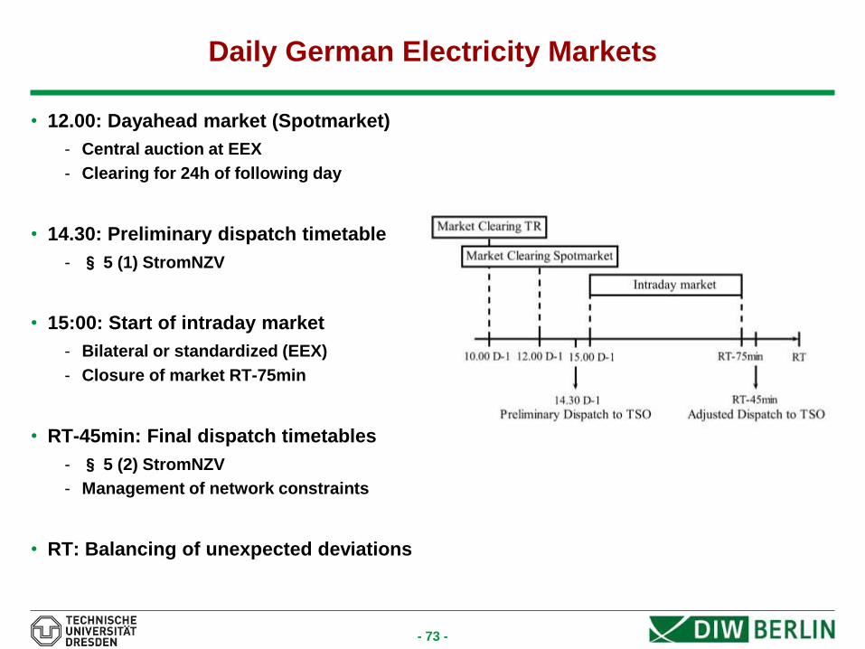
Daily German Electricity Markets
• 12.00: Dayahead market (Spotmarket)
- Central auction at EEX
- Clearing for 24h of following day
• 14.30: Preliminary dispatch timetable
- § 5 (1) StromNZV
• 15:00: Start of intraday market
- Bilateral or standardized (EEX)
- Closure of market RT-75min
• RT-45min: Final dispatch timetables
- § 5 (2) StromNZV
- Management of network constraints
• RT: Balancing of unexpected deviations
- 74 -
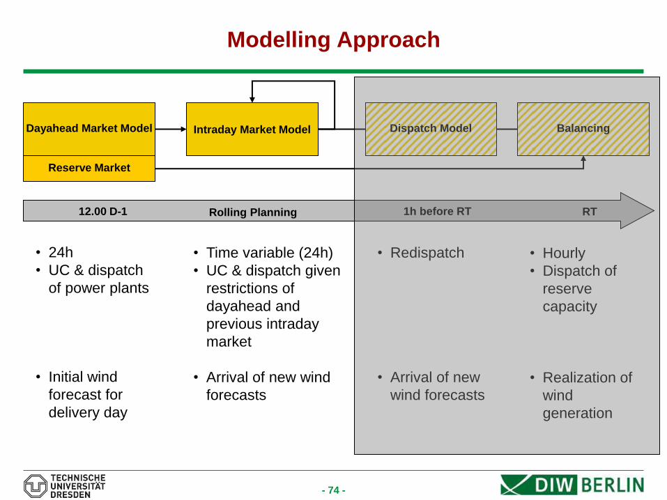
Modelling Approach
Dayahead Market Model Intraday Market Model
• 24h
• UC & dispatch
of power plants
• Initial wind
forecast for
delivery day
• Time variable (24h)
• UC & dispatch given
restrictions of
dayahead and
previous intraday
market
• Arrival of new wind
forecasts
• Redispatch
• Arrival of new
wind forecasts
• Hourly
• Dispatch of
reserve
capacity
• Realization of
wind
generation
12.00 D-1 1h before RT RT Rolling Planning
Reserve Market
Dispatch Model Balancing

- 75 -
Dayahead Market Model
Given: wind forecast, (past power plant plans)
Decide about: plant status, generation, reserve provision, storage use
min (Generation Cost + Startup Cost)
subject to:
Generation = Demand
Reserve Capacity = Reserve Demand
Generation <= Installed Capacity
Generation >= Minimum Generation (if online)
Offline Time >= Minimum Offline Time
Online Time >= Minimum Online Time
+ Storage restrictions, Wind Shedding
- 76 -
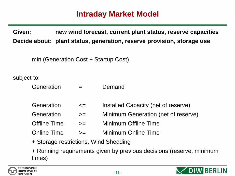
Intraday Market Model
Given: new wind forecast, current plant status, reserve capacities
Decide about: plant status, generation, reserve provision, storage use
min (Generation Cost + Startup Cost)
subject to:
Generation = Demand
Generation <= Installed Capacity (net of reserve)
Generation >= Minimum Generation (net of reserve)
Offline Time >= Minimum Offline Time
Online Time >= Minimum Online Time
+ Storage restrictions, Wind Shedding
+ Running requirements given by previous decisions (reserve, minimum
times)
- 77 -
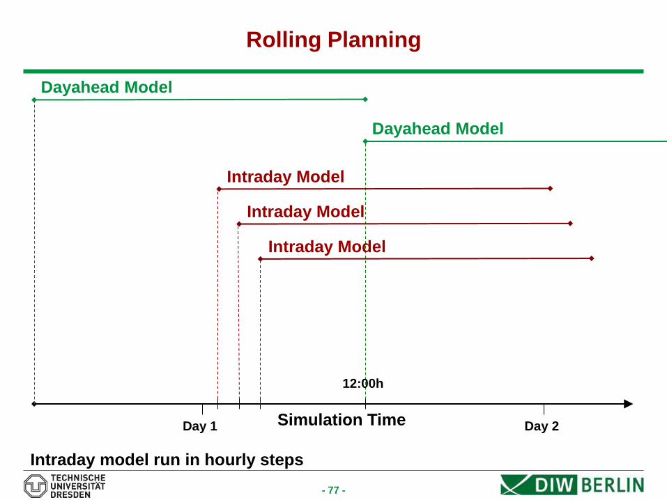
Rolling Planning
Simulation Time
Dayahead Model
Day 1 Day 2
12:00h
Dayahead Model
Intraday Model
Intraday Model
Intraday Model
Intraday model run in hourly steps

Thank you very much
for your attention!
Any questions or comments?
- 79 -
Literature
• S.A. Gabriel and F.U. Leuthold. Solving discretely-constrained MPEC
problems with applications in electric power markets. Energy Economics,
32(1):3–14, 2010.
• F.U. Leuthold, H. Weigt, and C. von Hirschhausen. A Large-Scale Spatial
Optimization Model of the European Electricity Market. Networks and Spatial
Economics, 2010.
• K. Neuhoff, J. Barquin, M.G. Boots, A. Ehrenmann, B.F. Hobbs, F.A. Rijkers,
and M. Vázquez. Network-constrained cournot models of liberalized
electricity markets: the devil is in the details. Energy Economics, 27(3):495 –
525, 2005.
• F.C. Schweppe, M.C. Caramanis, R.D. Tabors, and R. E. Bohn: Spot Pricing
of Electricity. Kluwer, Boston, 1988.
• H. Stigler and C. Todem. Optimization of the Austrian Electricity Sector
(Control Zone of VERBUND APG) under the Constraints of Network
Capacities by Nodal Pricing. Central European Journal of Operations
Research, 13:105–125, 2005.