Embed Size (px)
Citation preview

IntroductiontodiffusionNMR
MathiasNilsson
NMRMethodologyGroupUniversityofManchester
UNICAMP.Campinas,BrazilApril17th ,2018
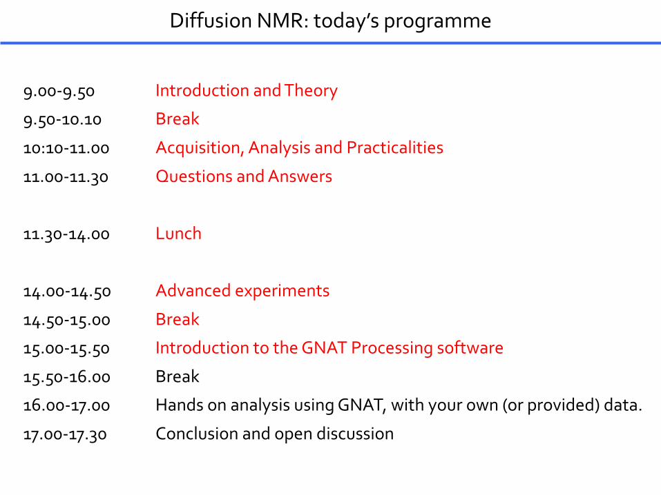
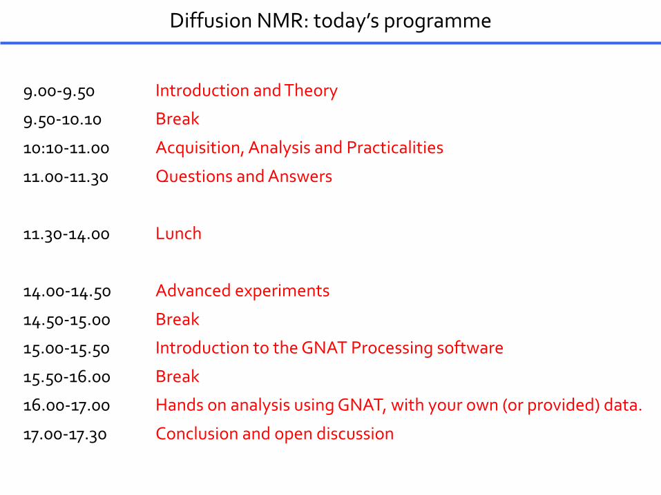
Diffusion NMR: today’s programme
9.00-9.50 Introduction and Theory
9.50-10.10 Break
10:10-11.00 Acquisition, Analysis and Practicalities
11.00-11.30 Questions and Answers
11.30-14.00 Lunch
14.00-14.50 Advanced experiments
14.50-15.00 Break
15.00-15.50 Introduction to the GNAT Processing software
15.50-16.00 Break
16.00-17.00 Hands on analysis using GNAT, with your own (or provided) data.
17.00-17.30 Conclusion and open discussion
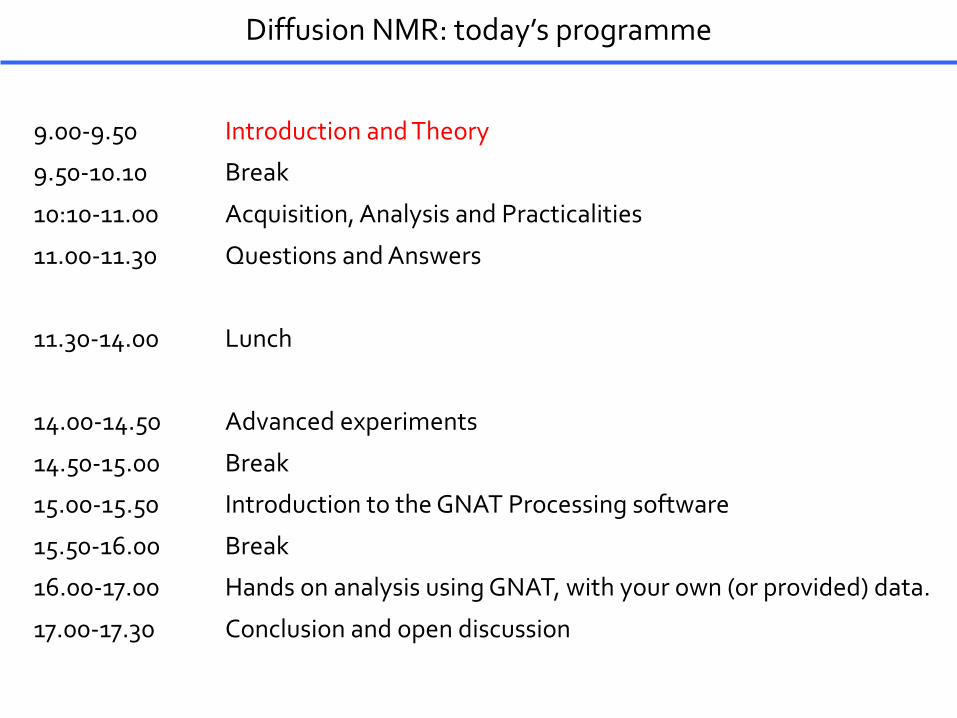
9 8 7 6 5 4 3 2 1 ppm
applicationsmetabolomicsdrug developmentprocess chemistryfood sciencenatural products chemistryorganic synthesis
500 MHz proton spectrum of port wine
pros/cons+ structural information + nondestructive− low(ish) sensitivity− usually needs separation (e.g. LC-NMR)
mixture analysis by NMR
789 ppm
J. Agric. Food Chem. 2004, 52, 3736
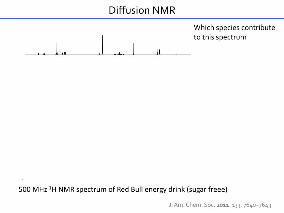
J. Am. Chem. Soc. 2011. 133, 7640–7643
By encoding diffusion into an NMR experiment, the individual component spectra can be identified.
tartrazineephedrine TSPnicotinic acid
ethanol
HOD
dextran
Diffusion NMRWhich species contribute to this spectrum
500MHz1HNMRspectrumofRedBullenergydrink(sugarfreee)
Diffusion NMR: information
Diffusion is central in much of chemistry and science in general. It is important in a
large variety of topics including mass transport, reactivity, kinetics, separation
science, nano-technology, hydrodynamics, inter-molecular dynamics, motional
restriction etc.
In this course we will focus directly on how to measure diffusion by NMR, how to
process the data and some of its applications:
Relative diffusion information -> separation/identification of NMR spectra from
different components in a mixture. Diffusion-ordered spectroscopy (DOSY)
Absolute diffusion information -> size estimation of molecules and aggregates
Manipulating diffusion -> identification of components and binding/interaction
RecommendedTexts
Claridge, High-Resolution NMR Techniques in Organic Chemistry, 3rd ed.,Elsevier, 2016 (Chapter 10 on Diffusion NMR)Callaghan, Translational Dynamics and Magnetic Resonance. Principles of Pulsed Gradient Spin Echo NMR. Oxford, 2011
Advancedtopics
Price,NMRStudiesofTranslationalMotion:PrinciplesandApplications,CambridgeUniversityPress,2009
Andreferencesgivenonslides
Diffusion NMR: suggested reading

Brownian motion
Molecules in solution move at random because of collisions. How far they move on
average in a given length of time t depends on the diffusion coefficient D: the root-
mean-square displacement for diffusion in three dimensions is 6Dt
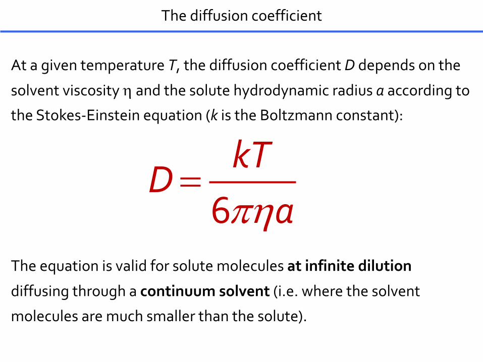
The diffusion coefficient
At a given temperature T, the diffusion coefficient D depends on the
solvent viscosity h and the solute hydrodynamic radius a according to
the Stokes-Einstein equation (k is the Boltzmann constant):
The equation is valid for solute molecules at infinite dilution
diffusing through a continuum solvent (i.e. where the solvent
molecules are much smaller than the solute).
ph=6kT
Da

the diffusion coefficient
The hydrodynamic radius a is the effective average radius of the solvated solute
molecules, and will depend on the molar mass MW. Assuming similar chemistries
(i.e. constant density)
• for a spherical molecule such as a globular protein,
• for a ‘random coil’ polymer or a flat disk,
• for a rigid linear molecule
In practice D will also depend on concentration, molecular shape, interactions etc.
ph=6kT
Da
( )-µ 1/3D MW
( )-µ 1/2D MW
( )-µ 1D MW
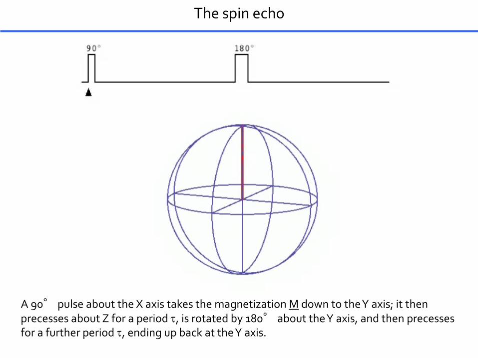
The spin echo
A 90° pulse about the X axis takes the magnetization M down to the Y axis; it then precesses about Z for a period t, is rotated by 180° about the Y axis, and then precessesfor a further period t, ending up back at the Y axis.
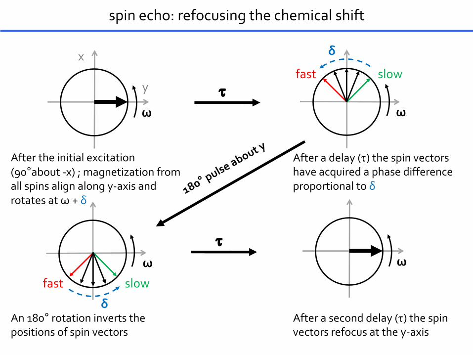
spin echo: refocusing the chemical shift
ω
ω
δ
ω
δ
After the initial excitation (90°about -x) ; magnetization from all spins align along y-axis and rotates at ω + δ
t
An 180° rotation inverts the positions of spin vectors
t
fast slow
fast slow
After a delay (t) the spin vectors have acquired a phase difference proportional to δ
ω
After a second delay (t) the spin vectors refocus at the y-axis
y
x
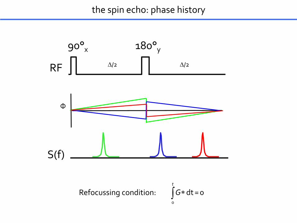
RF
S(f)
90°x 180°y
Φ
Refocussing condition:0
dt 0t
G =*ò
D/2 D/2
the spin echo: phase history

magnetic field gradients
direction of B0
magnitude of B0
low Larmorfrequency
The strength of the magnetic field is varied so that the Larmorfrequency is [linearly] dependent on z position.
gradient coils0
L zB= + G z
2gnp
high Larmorfrequency
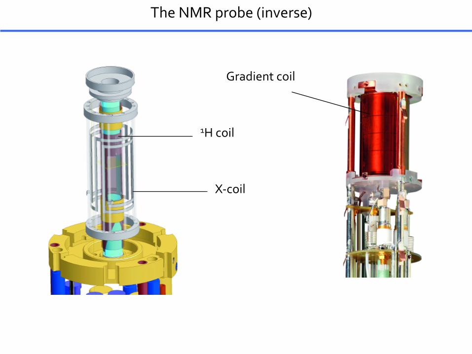
The NMR probe (inverse)
1H coil
X-coil
Gradient coil
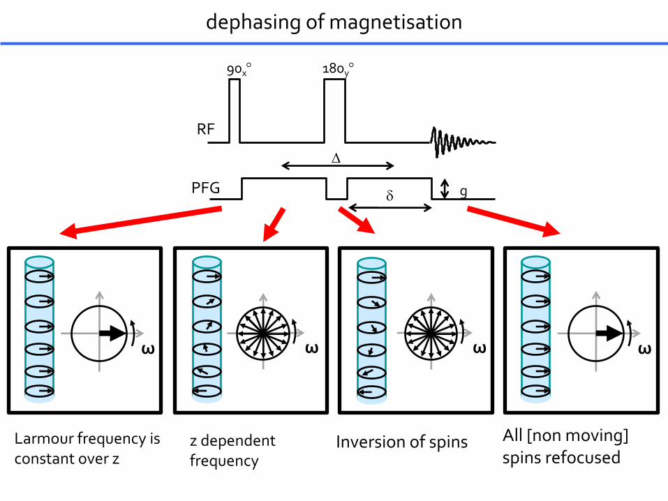
dephasing of magnetisation
RF
D
PFG d g
90x° 180y°
ω ω ω ω
Larmour frequency is constant over z
z dependent frequency
Inversion of spins All [non moving] spins refocused
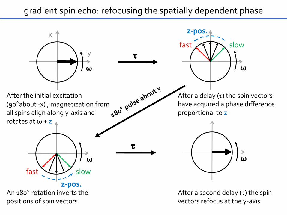
gradient spin echo: refocusing the spatially dependent phase
ω
ω
z-pos.
ω
z-pos.
After the initial excitation (90°about -x) ; magnetization from all spins align along y-axis and rotates at ω + z
t
An 180° rotation inverts the positions of spin vectors
t
fast slow
fast slow
After a delay (t) the spin vectors have acquired a phase difference proportional to z
ω
After a second delay (t) the spin vectors refocus at the y-axis
y
x
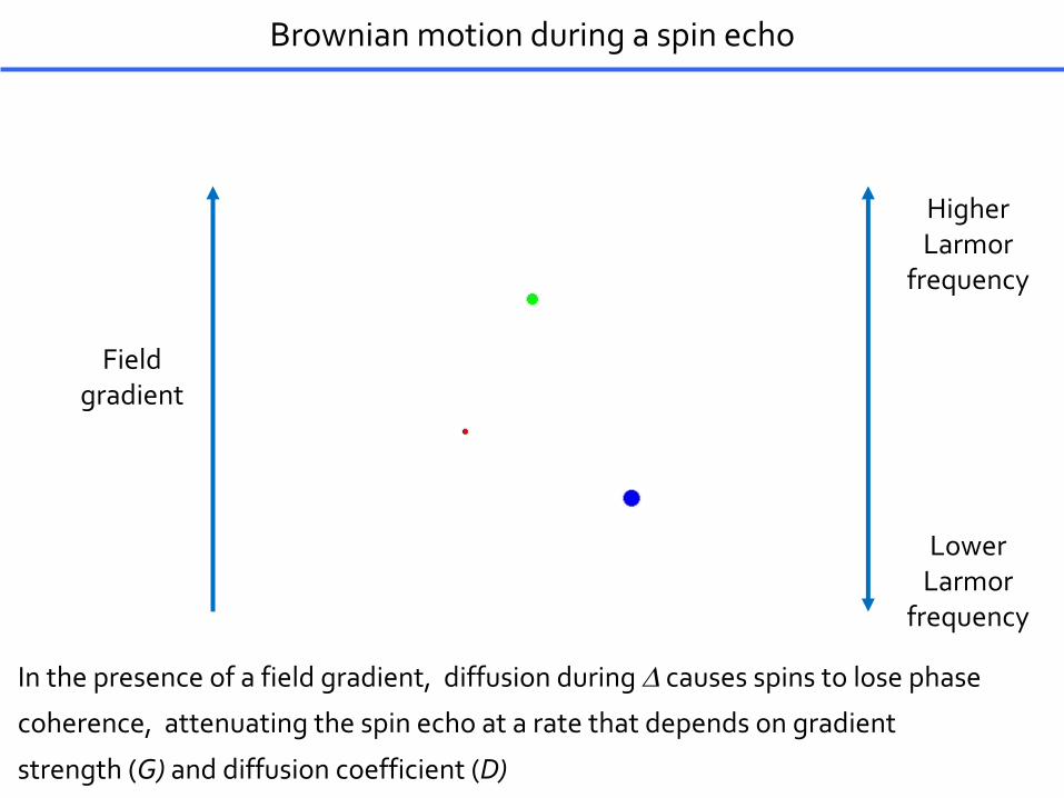
Brownian motion during a spin echo
Fieldgradient
HigherLarmor
frequency
LowerLarmor
frequency
In the presence of a field gradient, diffusion during D causes spins to lose phase
coherence, attenuating the spin echo at a rate that depends on gradient
strength (G) and diffusion coefficient (D)
Fieldgradient
higher Larmorfrequency
lower Larmorfrequency
f
f
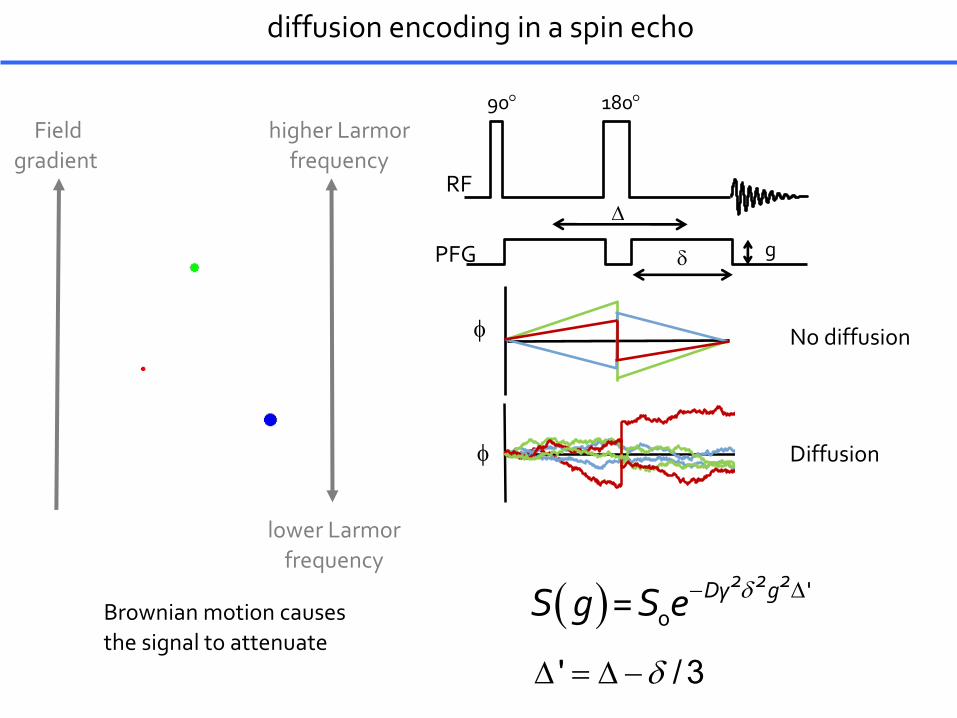
diffusion encoding in a spin echo
Brownian motion causes the signal to attenuate
Diffusion
No diffusion
( ) d- D'0
2 2 2Dγ gS g =S e
RFD
PFG d g
90° 180°
' / 3dD = D -
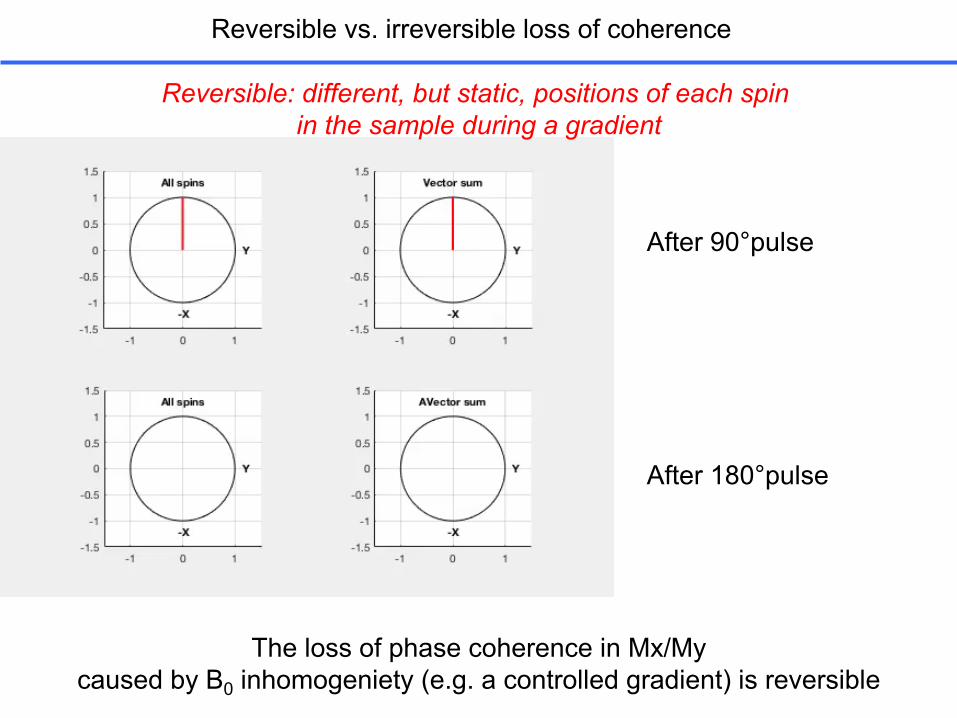
Reversible vs. irreversible loss of coherence
The loss of phase coherence in Mx/My caused by B0 inhomogeniety (e.g. a controlled gradient) is reversible
After 90°pulse
After 180°pulse
Reversible: different, but static, positions of each spin in the sample during a gradient
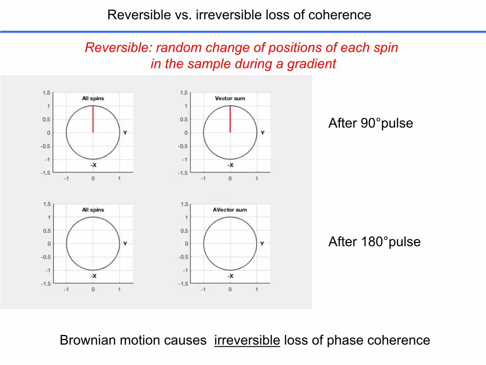
Brownian motion causes irreversible loss of phase coherence
Reversible vs. irreversible loss of coherence
After 90°pulse
After 180°pulse
Reversible: random change of positions of each spin in the sample during a gradient
Reversible vs. irreversible loss of coherence
After 90°pulse
After 180°pulse
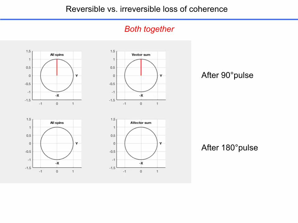
Both together
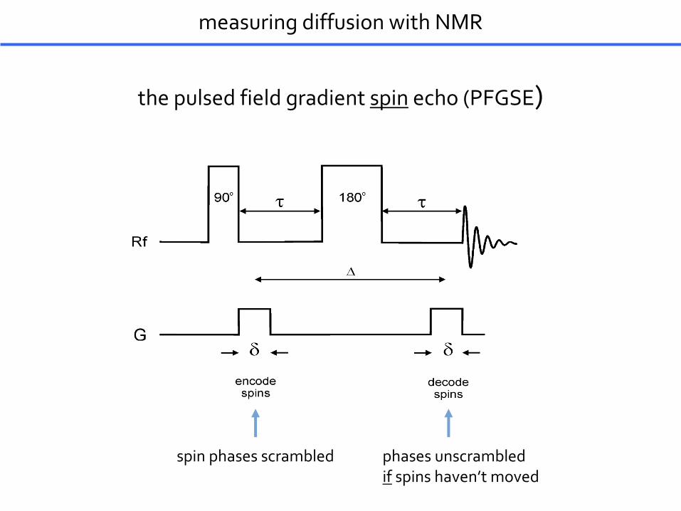
measuring diffusion with NMR
spin phases scrambled phases unscrambledif spins haven’t moved
the pulsed field gradient spin echo (PFGSE)

pulse sequences
A practical pulse sequence: “Oneshot”
needs only 1 transient per increment; minimum time < 1 min
( ) d- D '0
2 2 2Dγ gS g =S e
Magn. Reson. Chem. 2002, 40, S147
2 2( 2) ( 1)' 6 2
d a t a- -D = D - -
D
90° 180°
1+α
1-α 2αd/2

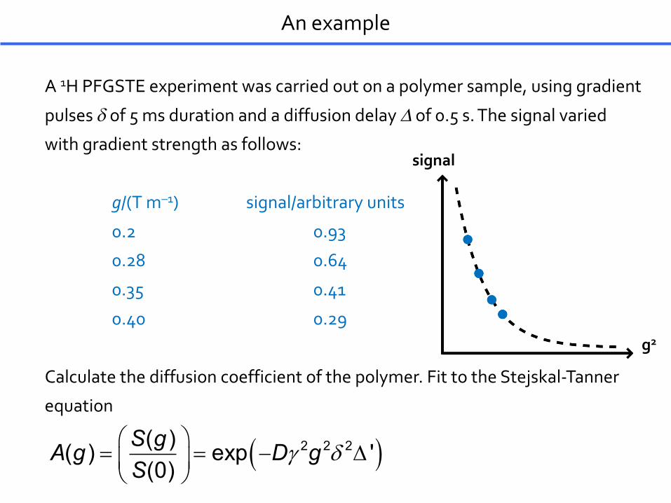
A 1H PFGSTE experiment was carried out on a polymer sample, using gradient
pulses d of 5 ms duration and a diffusion delay D of 0.5 s. The signal varied
with gradient strength as follows:
g/(T m–1) signal/arbitrary units
0.2 0.93
0.28 0.64
0.35 0.41
0.40 0.29
Calculate the diffusion coefficient of the polymer. Fit to the Stejskal-Tanner
equation
An example
( )2 2 2( )( ) exp '(0)S gA g D gS
g dæ ö= = - Dç ÷è ø
g2
signal
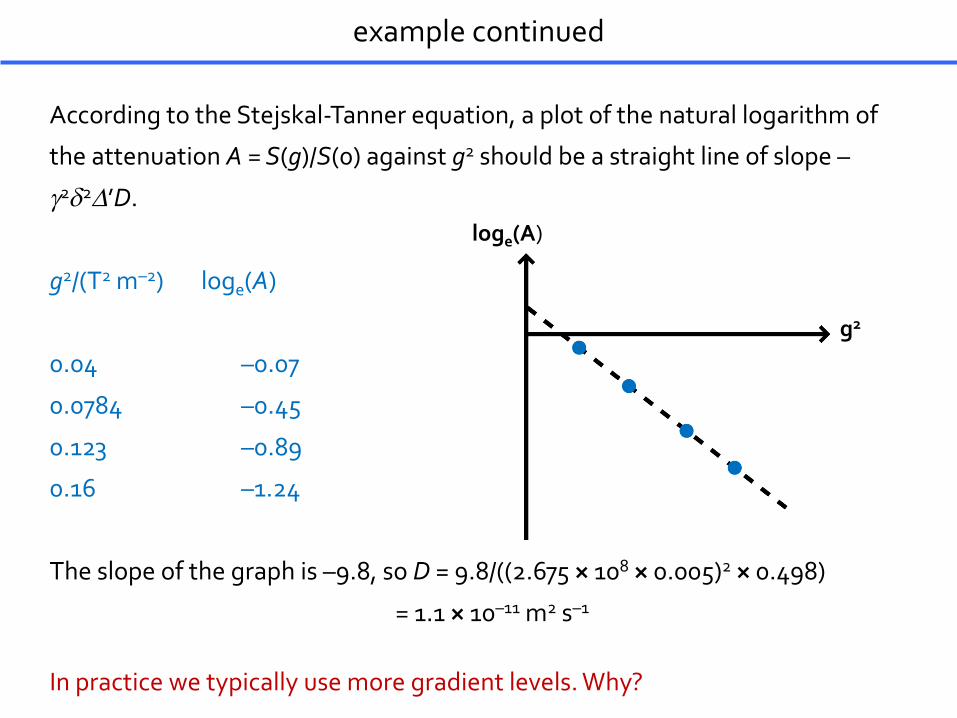
According to the Stejskal-Tanner equation, a plot of the natural logarithm of
the attenuation A = S(g)/S(0) against g2 should be a straight line of slope –
g2d2D’D.
g2/(T2 m–2) loge(A)
0.04 –0.07
0.0784 –0.45
0.123 –0.89
0.16 –1.24
The slope of the graph is –9.8, so D = 9.8/((2.675 × 108 × 0.005)2 × 0.498)
= 1.1 × 10⁻¹¹ m2 s–1
In practice we typically use more gradient levels. Why?
example continued
loge(A)
g2
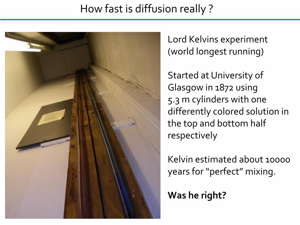
How fast is diffusion really ?
Lord Kelvins experiment(world longest running)
Started at University of Glasgow in 1872 using5.3 m cylinders with one differently colored solution in the top and bottom half respectively
Kelvin estimated about 10000 years for “perfect” mixing.
Was he right?
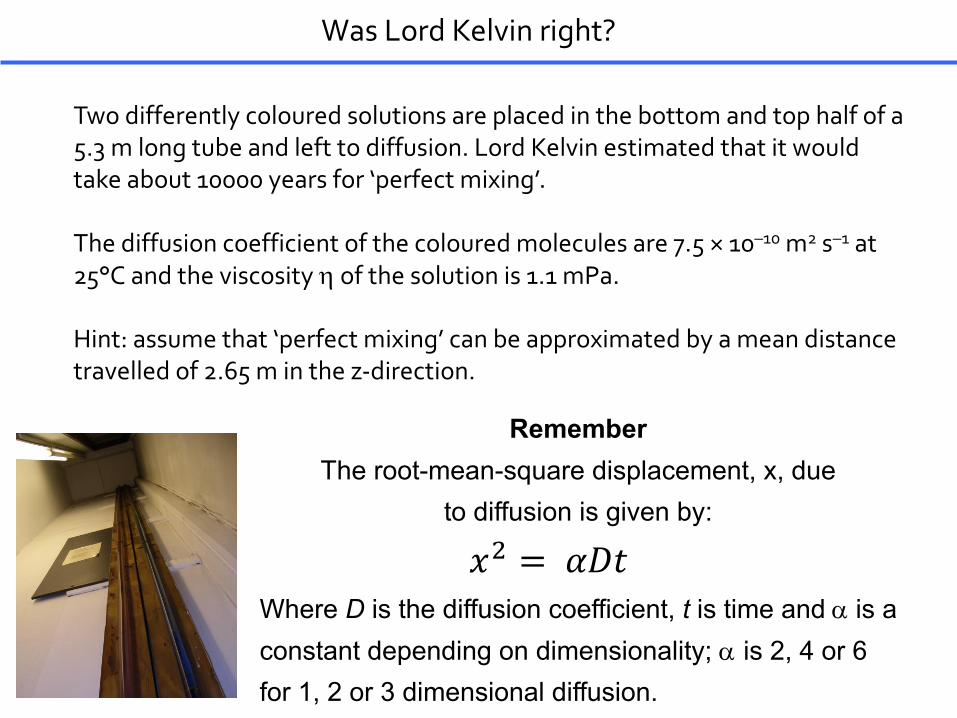
Two differently coloured solutions are placed in the bottom and top half of a 5.3 m long tube and left to diffusion. Lord Kelvin estimated that it would take about 10000 years for ‘perfect mixing’.
The diffusion coefficient of the coloured molecules are 7.5 × 10⁻¹⁰ m2 s–1 at 25°C and the viscosity h of the solution is 1.1 mPa.
Hint: assume that ‘perfect mixing’ can be approximated by a mean distance travelled of 2.65 m in the z-direction.
Was Lord Kelvin right?
RememberThe root-mean-square displacement, x, due
to diffusion is given by:
𝑥" = 𝛼𝐷𝑡Where D is the diffusion coefficient, t is time and a is a constant depending on dimensionality; a is 2, 4 or 6 for 1, 2 or 3 dimensional diffusion.
Was Lord Kelvin right?
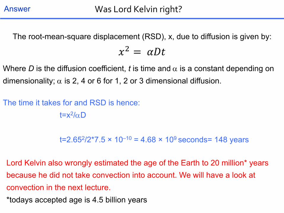
The root-mean-square displacement (RSD), x, due to diffusion is given by:
𝑥" = 𝛼𝐷𝑡Where D is the diffusion coefficient, t is time and a is a constant depending on dimensionality; a is 2, 4 or 6 for 1, 2 or 3 dimensional diffusion.
The time it takes for and RSD is hence:t=x2/aD
t=2.652/2*7.5 × 10–10 = 4.68 × 10⁹ seconds= 148 years
Answer
Lord Kelvin also wrongly estimated the age of the Earth to 20 million* years because he did not take convection into account. We will have a look at convection in the next lecture.*todays accepted age is 4.5 billion years
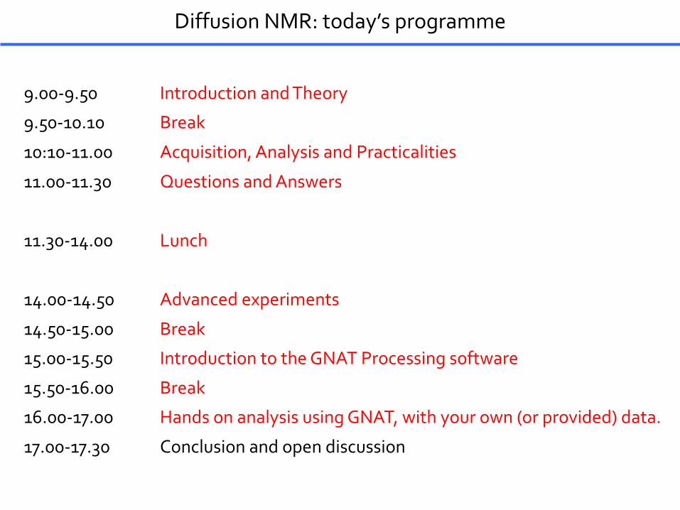
Diffusion NMR: today’s programme
9.00-9.50 Introduction and Theory
9.50-10.10 Break
10:10-11.00 Acquisition, Analysis and Practicalities
11.00-11.30 Questions and Answers
11.30-14.00 Lunch
14.00-14.50 Advanced experiments
14.50-15.00 Break
15.00-15.50 Introduction to the GNAT Processing software
15.50-16.00 Break
16.00-17.00 Hands on analysis using GNAT, with your own (or provided) data.
17.00-17.30 Conclusion and open discussion
A 1H PFGSTE experiment was carried out on a polymer sample, using gradient
pulses d of 5 ms duration and a diffusion delay D of 0.5 s. The signal varied
with gradient strength as follows:
g/(T m–1) signal/arbitrary units
0.2 0.93
0.28 0.64
0.35 0.41
0.40 0.29
Calculate the diffusion coefficient of the polymer. Fit to the Stejskal-Tanner
equation
An example
( )2 2 2( )( ) exp '(0)S gA g D gS
g dæ ö= = - Dç ÷è ø
g2
signal
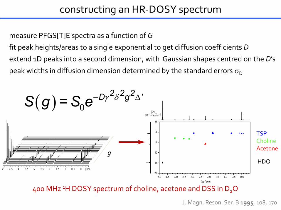
measure PFGS[T]E spectra as a function of G
fit peak heights/areas to a single exponential to get diffusion coefficients D
extend 1D peaks into a second dimension, with Gaussian shapes centred on the D’s
peak widths in diffusion dimension determined by the standard errors sD
400 MHz 1H DOSY spectrum of choline, acetone and DSS in D2O
TSPCholineAcetone
gHDO
constructing an HR-DOSY spectrum
J. Magn. Reson. Ser. B 1995, 108, 170
( ) '0
2 2 2D gS g = S e g d- D
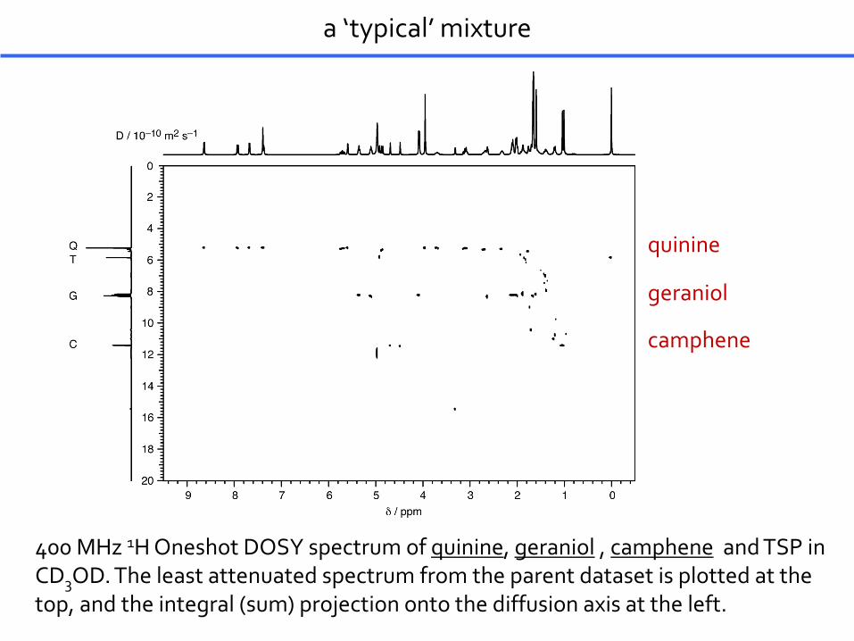
400 MHz 1H Oneshot DOSY spectrum of quinine, geraniol , camphene and TSP in CD3OD. The least attenuated spectrum from the parent dataset is plotted at the top, and the integral (sum) projection onto the diffusion axis at the left.
quinine
camphene
geraniol
a ‘typical’ mixture
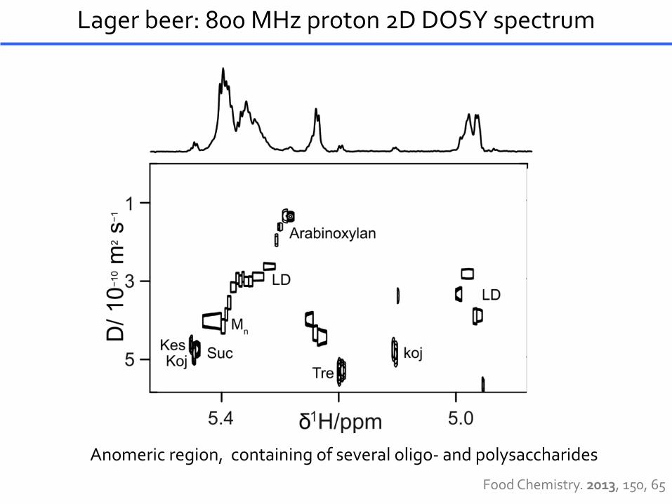
Anomeric region, containing of several oligo- and polysaccharides
Lager beer: 800 MHz proton 2D DOSY spectrum
Food Chemistry. 2013, 150, 65
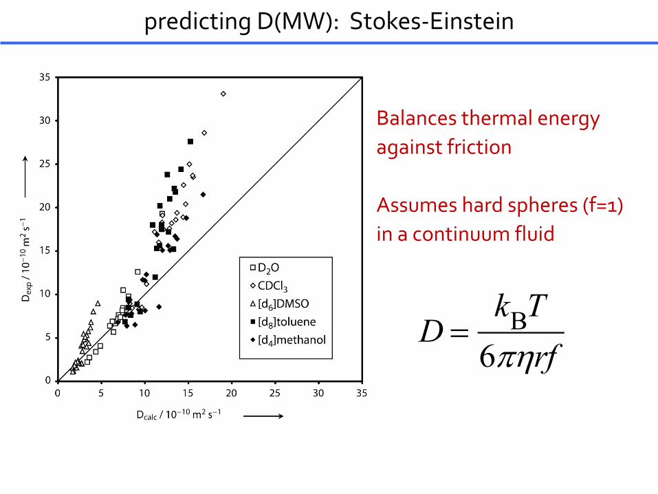
Balances thermal energy against friction
Assumes hard spheres (f=1) in a continuum fluid
D =
kBT6phrf
predicting D(MW): Stokes-Einstein

A constant effective density for all solutes
Combines theoretical and empirical approaches
Relatives sizes of solvent and solute molecules are used
D =kBT 3a
2+
11+a
æèç
öø÷
6ph 3MW4preff N A
3
, where a =MWsMW
3
predicting D(MW): proposed alternative
Angew. Chem. Int. Ed. 2013, 52, 3199
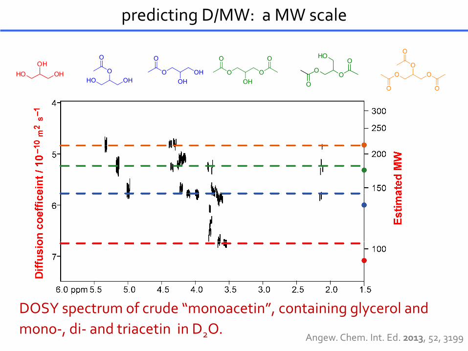
DOSY spectrum of crude “monoacetin”, containing glycerol and mono-, di- and triacetin in D2O.
predicting D/MW: a MW scale
OHOH
HO OO
HOO
O
Angew. Chem. Int. Ed. 2013, 52, 3199
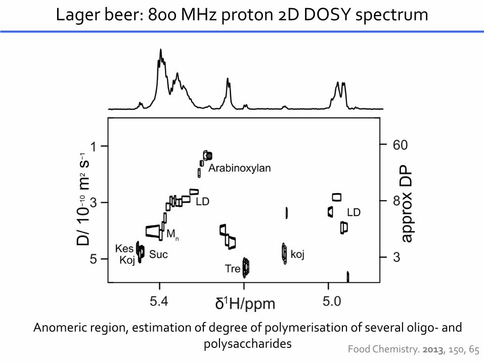
Anomeric region, estimation of degree of polymerisation of several oligo- and polysaccharides
Lager beer: 800 MHz proton 2D DOSY spectrum
Food Chemistry. 2013, 150, 65
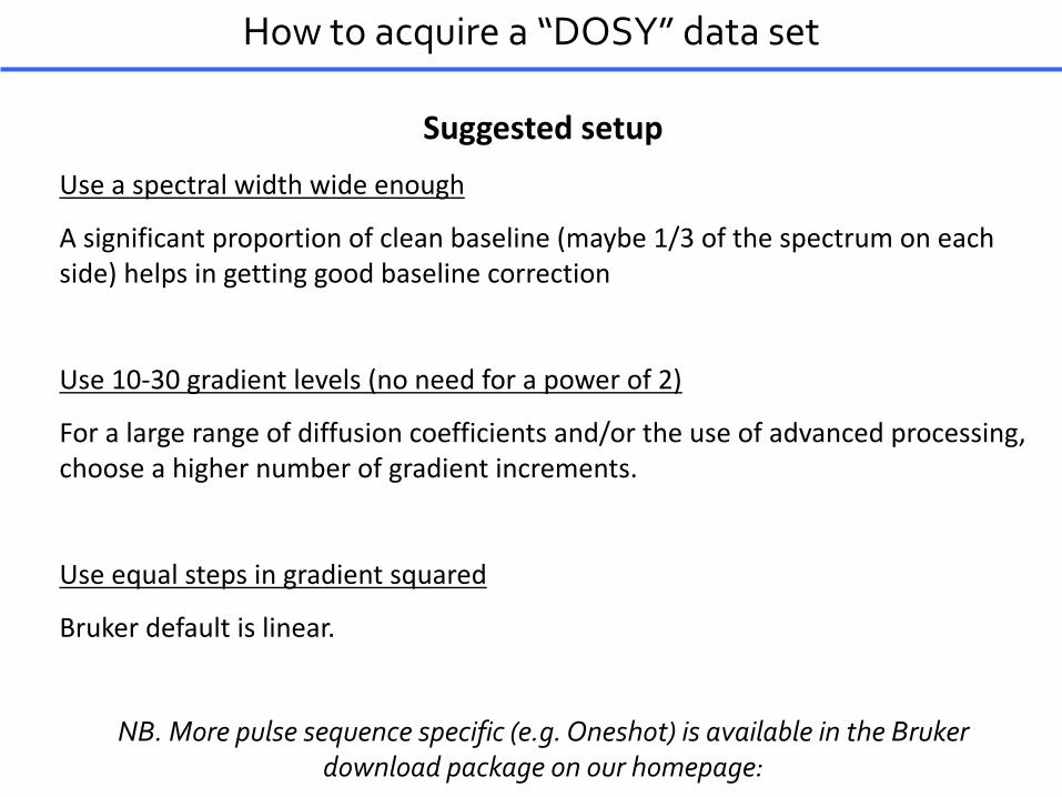
How to acquire a “DOSY” data set
NB. More pulse sequence specific (e.g. Oneshot) is available in the Bruker download package on our homepage:
SuggestedsetupUseaspectralwidthwideenough
Asignificantproportionofcleanbaseline(maybe1/3ofthespectrumoneachside)helpsingettinggoodbaselinecorrection
Use10-30gradientlevels(noneedforapowerof2)
Foralargerangeofdiffusioncoefficientsand/ortheuseofadvancedprocessing,chooseahighernumberofgradientincrements.
Useequalstepsingradientsquared
Brukerdefaultislinear.
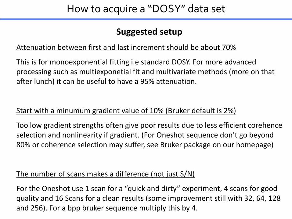
How to acquire a “DOSY” data set
SuggestedsetupAttenuationbetweenfirstandlastincrementshouldbeabout70%
Thisisformonoexponential fittingi.e standardDOSY.Formoreadvancedprocessingsuchasmultiexponetial fitandmultivariatemethods(moreonthatafterlunch)itcanbeusefultohavea95%attenuation.
Startwithaminumum gradientvalueof10%(Brukerdefaultis2%)
Toolowgradientstrengthsoftengivepoorresultsduetolessefficientcorehenceselectionandnonlinearityifgradient.(ForOneshot sequencedon’tgobeyond80%orcoherenceselectionmaysuffer,seeBrukerpackageonourhomepage)
Thenumberofscansmakesadifference(notjustS/N)
FortheOneshot use1scanfora“quickanddirty”experiment,4scansforgoodqualityand16Scansforacleanresults(someimprovementstillwith32,64,128and256).Forabpp bruker sequencemultiplythisby4.
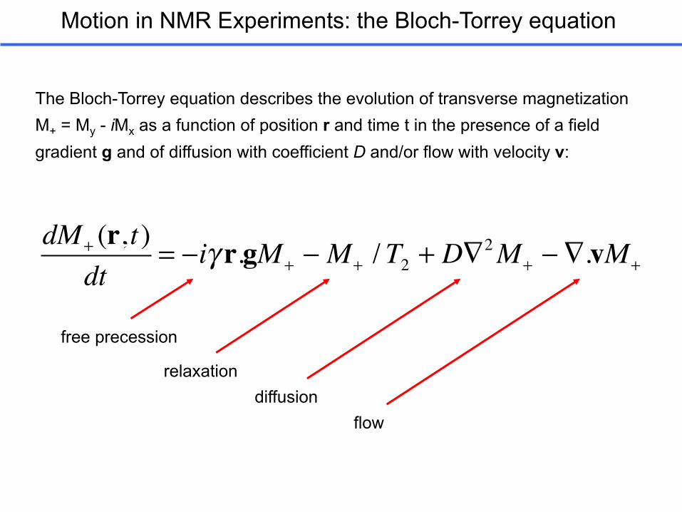
Motion in NMR Experiments: the Bloch-Torrey equation
dM + (r, t)dt
= −iγ r.gM + − M+ / T2 + D∇2M+ − ∇.vM+
The Bloch-Torrey equation describes the evolution of transverse magnetization M+ = My - iMx as a function of position r and time t in the presence of a field gradient g and of diffusion with coefficient D and/or flow with velocity v:
free precession
relaxationdiffusion
flow
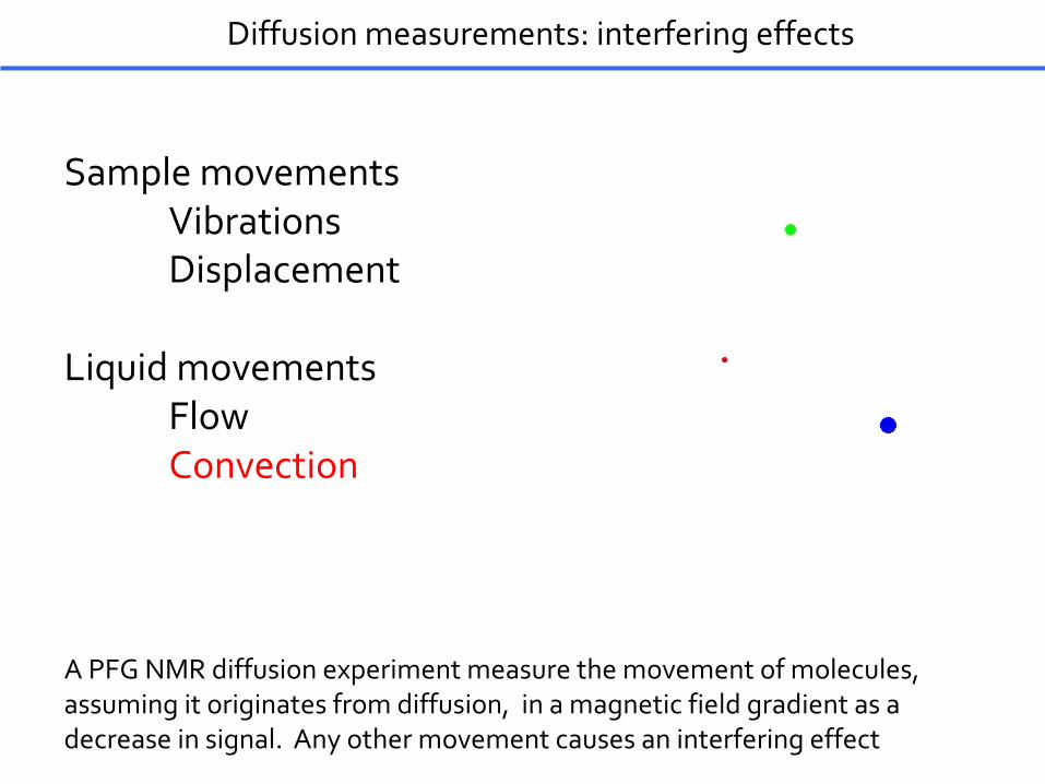
Sample movementsVibrationsDisplacement
Liquid movementsFlowConvection
Diffusion measurements: interfering effects
A PFG NMR diffusion experiment measure the movement of molecules, assuming it originates from diffusion, in a magnetic field gradient as a decrease in signal. Any other movement causes an interfering effect

Diffusion measurements: convection
Convection can occur when a system has different temperatures in different parts and the system strives towards equilibrium.
Convection in a heated pot
Convection at the sea/land interface
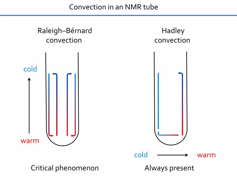
cold
warm
cold warm
Raleigh–Bérnardconvection
Critical phenomenon
Hadleyconvection
Always present
Convection in an NMR tube

Stejskal-Tanner equation modified for convection flow in an NMR tube
Where g is the magnetogyric ratio, g is the gradient pulse amplitude, and d is the gradient pulse width. D’ is the effective diffusion and flow time and v is the flow velocity
Convection in an NMR tube
𝑆(𝑔) = 𝑆,𝑒./01213145 cos𝐷𝛾𝛿𝑔Δ<𝑣
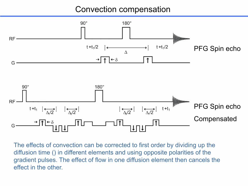
Convection compensation
PFG Spin echo
PFG Spin echo
Compensated
The effects of convection can be corrected to first order by dividing up the diffusion time () in different elements and using opposite polarities of the gradient pulses. The effect of flow in one diffusion element then cancels the effect in the other.

Convection compensation: pulse sequences
Double stimulated echo: lose 50% of signal and more phase cycling
Spin echo: no loss of signal or increased need for phase cycling
2DJ-IDOSY
PFGDSTE - CompensatedOneshot
2DJ-IDOSY - CompensatedJ. Magn. Reson. 177, 203 (2005)
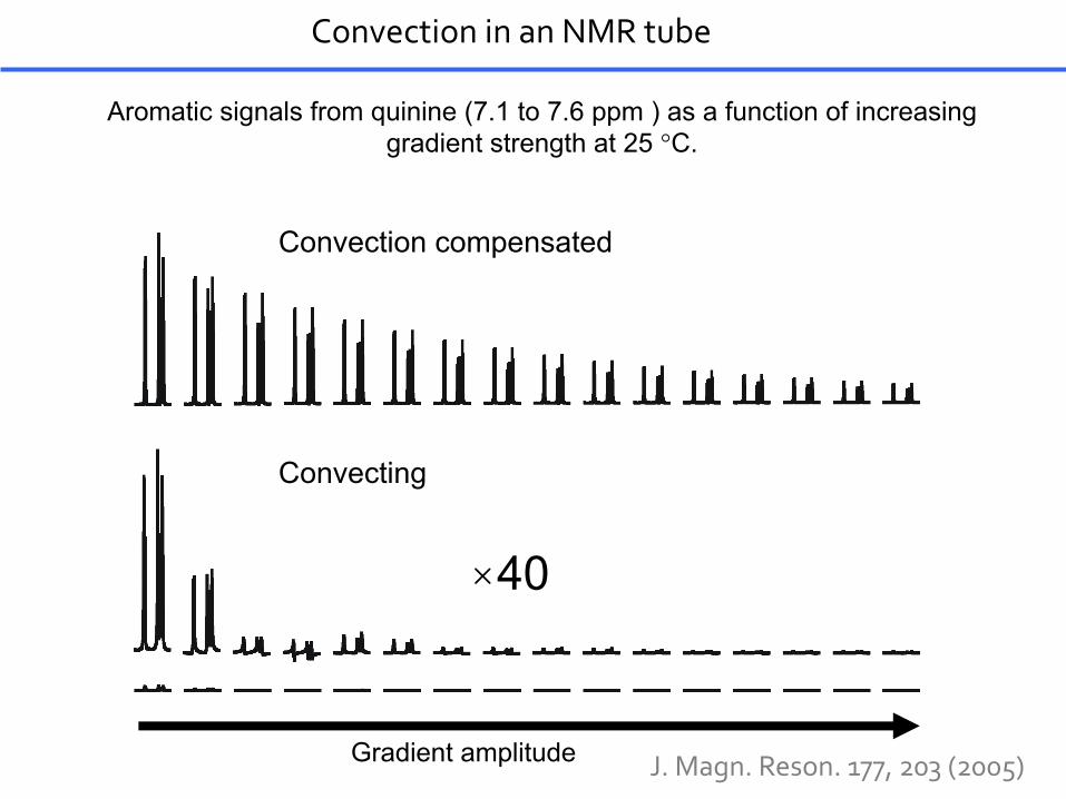
Aromatic signals from quinine (7.1 to 7.6 ppm ) as a function of increasing gradient strength at 25 °C.
Convection compensated
×40
Convecting
Gradient amplitude
Convection in an NMR tube
J. Magn. Reson. 177, 203 (2005)
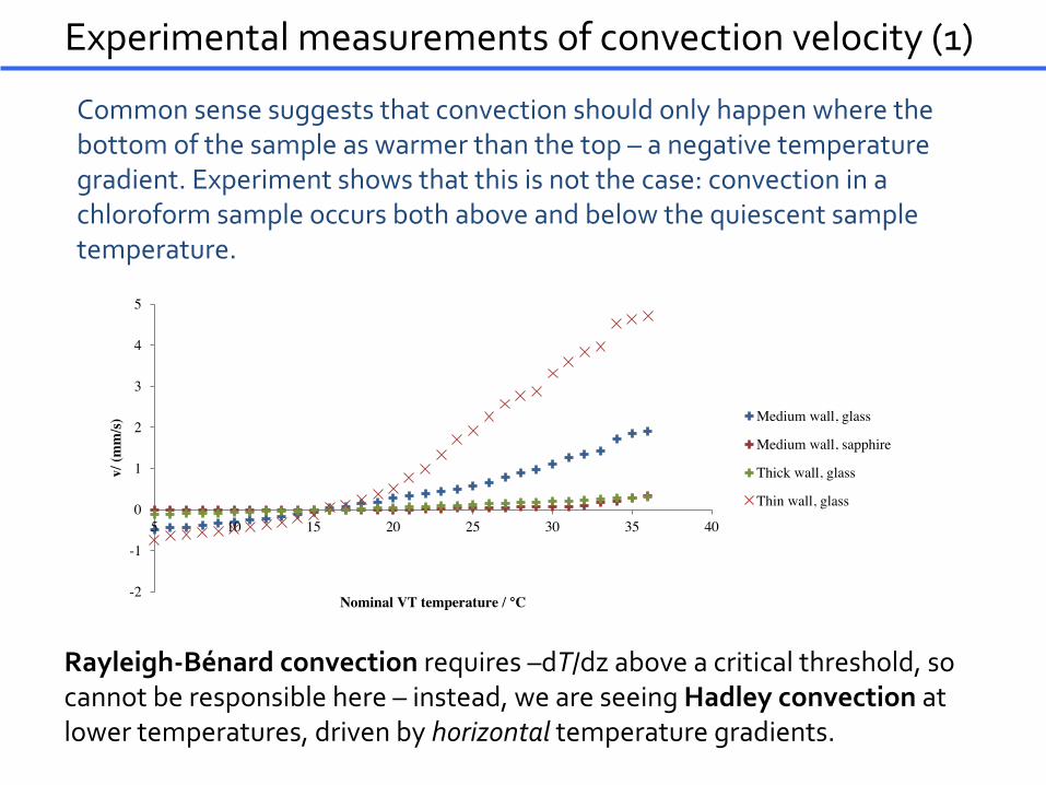
Experimental measurements of convection velocity (1)
Common sense suggests that convection should only happen where the bottom of the sample as warmer than the top – a negative temperature gradient. Experiment shows that this is not the case: convection in a chloroform sample occurs both above and below the quiescent sample temperature.
Rayleigh-Bénard convection requires –dT/dz above a critical threshold, so cannot be responsible here – instead, we are seeing Hadley convection at lower temperatures, driven by horizontal temperature gradients.
-2
-1
0
1
2
3
4
5
5 10 15 20 25 30 35 40
v/ (m
m/s)
Nominal VT temperature / °C
Medium wall, glass
Medium wall, sapphire
Thick wall, glass
Thin wall, glass
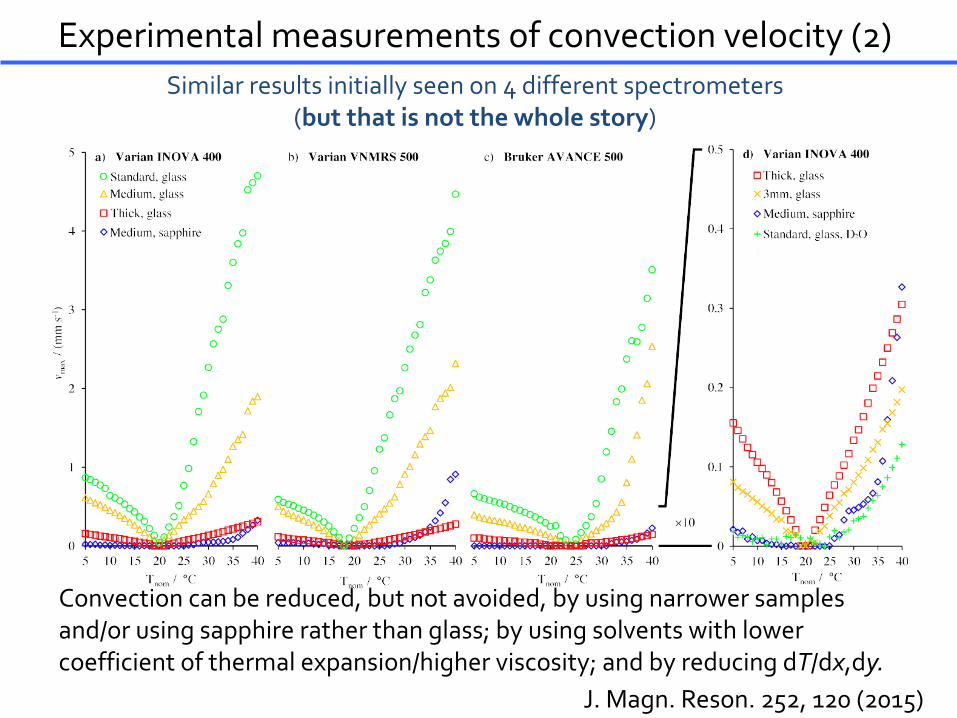
Experimental measurements of convection velocity (2)Similar results initially seen on 4 different spectrometers
(but that is not the whole story)
Convection can be reduced, but not avoided, by using narrower samples and/or using sapphire rather than glass; by using solvents with lower coefficient of thermal expansion/higher viscosity; and by reducing dT/dx,dy.
J. Magn. Reson. 252, 120 (2015)

Other probes/spectrometers show more florid behavior(all chloroform samples)
In some probes convection is always present at a problematic level (for a standard 5 mm tube using chloroform as solvent). It is still obvious that using a a restricted sample diameter suppresses convection very efficiently.
Experimental measurements of convection velocity (3)
RSC Advances. 6, 95173 (2016)
How to minimise convection
Useasmall(inner)diametertube
Thisisprobablythemosteffectivemethod,butcostsyou(typically50%)insensitivity.A3mmtubeorathick-walled5mmtubearegoodchoices.
Useamoreviscoussolvent
D2OandDMSOaregoodchoice.Solventlikechloroformconvects very easily
TurnoftheVTcontrol(Notforcryoprobes!)
Leavingtheprobetoequilibrateaquiescenttemperatureminimizestemperaturegradients.
Restrictthesampleheight
E.g.usingaShigemi tube.Significantlylesseffectivethanasmalldiameterbutpreservesmoresignal.
How to minimise convection
Useasapphiretube
Expensivebutthehighheatconductivityhelpsreducetemperaturegradients.
IncreasetheVTairflow
Helpsreducetemperaturegradients,butvibrationscandisturbthemeasurements.
Spinthesample
Veryefficient(reducestemperaturegradients),butoftengivesmessyresultsifthesequencetimingisnotmatchedwiththerotationfrequency.
Useconvectioncompensatedsequences
“Lastresort”e.g.forhighandlowtemperatureexperiments.Goodbutnotperfectcompensation.Costs50%insensitivityandrequiresalot(64scans)phasecycling.
Diffusion NMR: today’s programme
9.00-9.50 Introduction and Theory
9.50-10.10 Break
10:10-11.00 Acquisition, Analysis and Practicalities
11.00-11.30 Questions and Answers
11.30-14.00 Lunch
14.00-14.50 Advanced experiments
14.50-15.00 Break
15.00-15.50 Introduction to the GNAT Processing software
15.50-16.00 Break
16.00-17.00 Hands on analysis using GNAT, with your own (or provided) data.
17.00-17.30 Conclusion and open discussion

Anomeric region, estimation of degree of polymerisation of several oligo- and polysaccharides
Lager beer: 800 MHz proton 2D DOSY spectrum
Food Chemistry. 2013, 150, 65

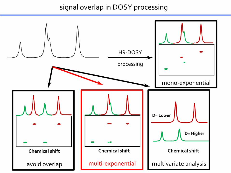
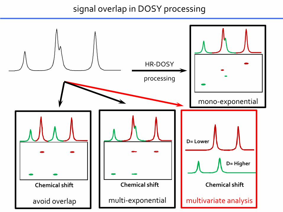
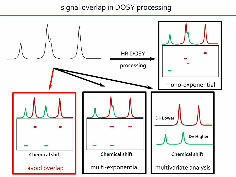
signal overlap in DOSY processing
HR-DOSY
processing
avoid overlap
Chemical shift
multivariate analysis
D= Lower
D= Higher
Chemical shiftChemical shift
multi-exponential
mono-exponential
signal overlap in DOSY processing
HR-DOSY
processing
avoid overlap
Chemical shift
multivariate analysis
D= Lower
D= Higher
Chemical shiftChemical shift
multi-exponential
mono-exponential

Resolving superimposed exponentials
Experimental (noisy) biexponential decay
Superimposed exponentials is a very difficult mathematical problem (ill-posed and numerically unstable). It is only practically feasible with high signal to noise ratio and for a limited (2-3) number of exponentials.
Residuals:
monoexponential fit
biexponential fitonly noise remaining
Chemical shift
Residuals (E) are the fit (F) subtracted from the experimental data (X)
R = X-F
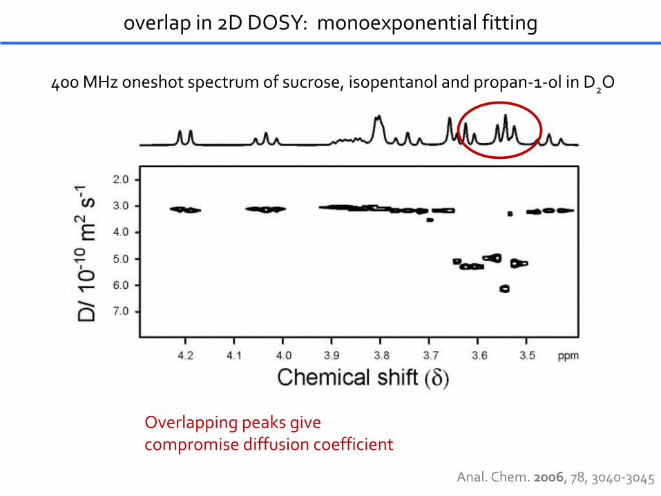
400 MHz oneshot spectrum of sucrose, isopentanol and propan-1-ol in D2O
overlap in 2D DOSY: monoexponential fitting
Anal. Chem. 2006, 78, 3040-3045
Overlapping peaks give compromise diffusion coefficient
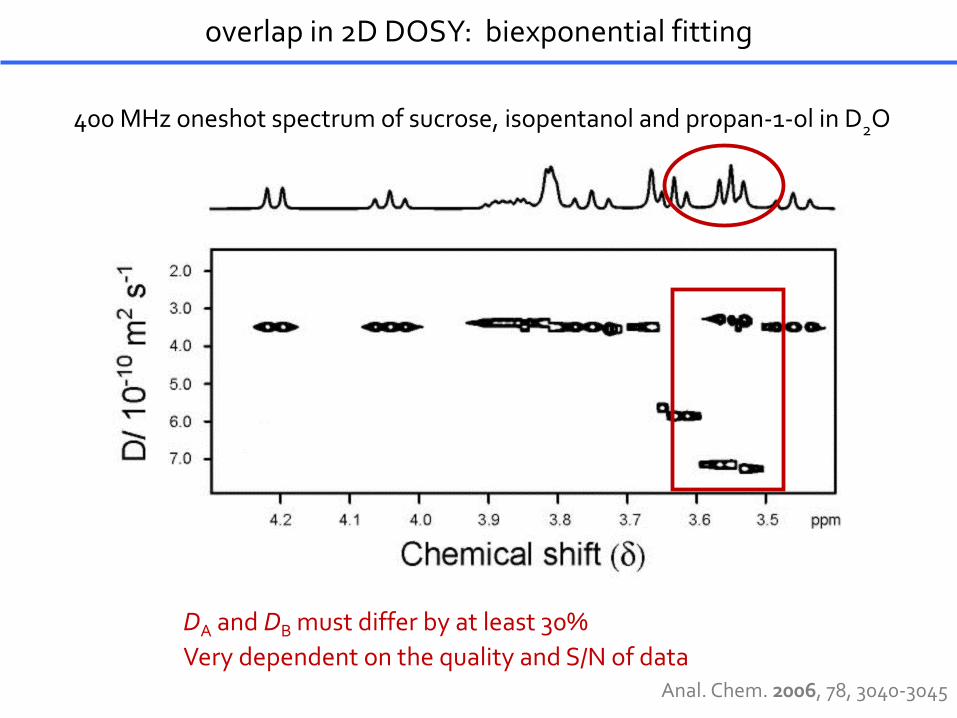
DA and DB must differ by at least 30%Very dependent on the quality and S/N of data
overlap in 2D DOSY: biexponential fitting
Anal. Chem. 2006, 78, 3040-3045
400 MHz oneshot spectrum of sucrose, isopentanol and propan-1-ol in D2O
signal overlap in DOSY processing
HR-DOSY
processing
avoid overlap
Chemical shift
multivariate analysis
D= Lower
D= Higher
Chemical shiftChemical shift
multi-exponential
mono-exponential
multivariate
decomposition
DOSY data (X) decays (C) spectra (S)
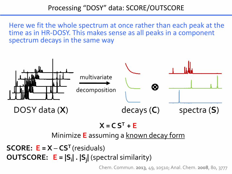
Processing“DOSY”data:SCORE/OUTSCORE
Chem. Commun. 2013, 49, 10510; Anal. Chem. 2008, 80, 3777
X = C ST + E Minimize E assuming a known decay form
Ä
SCORE: E = X – CST (residuals)OUTSCORE: E = |Si| . |Sj| (spectral similarity)
HerewefitthewholespectrumatonceratherthaneachpeakatthetimeasinHR-DOSY.Thismakessenseasallpeaksinacomponentspectrumdecaysinthesameway
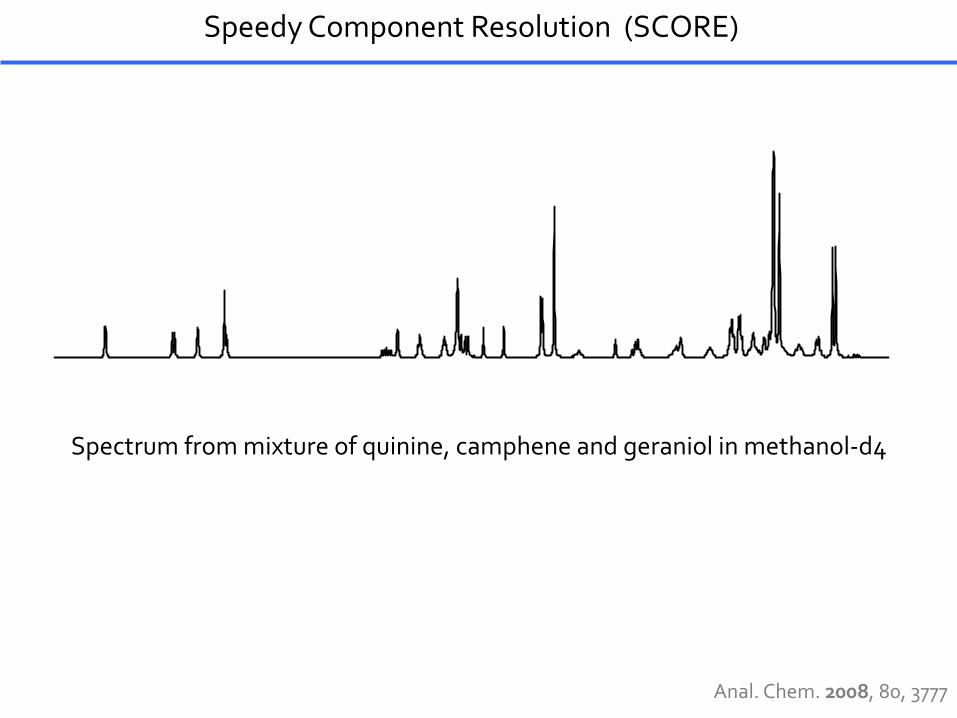
Spectrum from mixture of quinine, camphene and geraniol in methanol-d4
Speedy Component Resolution (SCORE)
Anal. Chem. 2008, 80, 3777
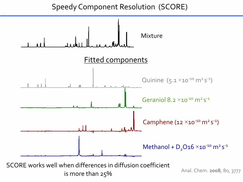
Quinine (5.1 ×10⁻¹⁰ m2 s-1)
Geraniol 8.2 ×10⁻¹⁰ m2 s-1
Camphene (12 ×10-10 m2 s-1)
Methanol + D2O16 ×10-10 m2 s-1
Speedy Component Resolution (SCORE)
Anal. Chem. 2008, 80, 3777SCORE works well when differences in diffusion coefficient
is more than 25%
Mixture
Fitted components
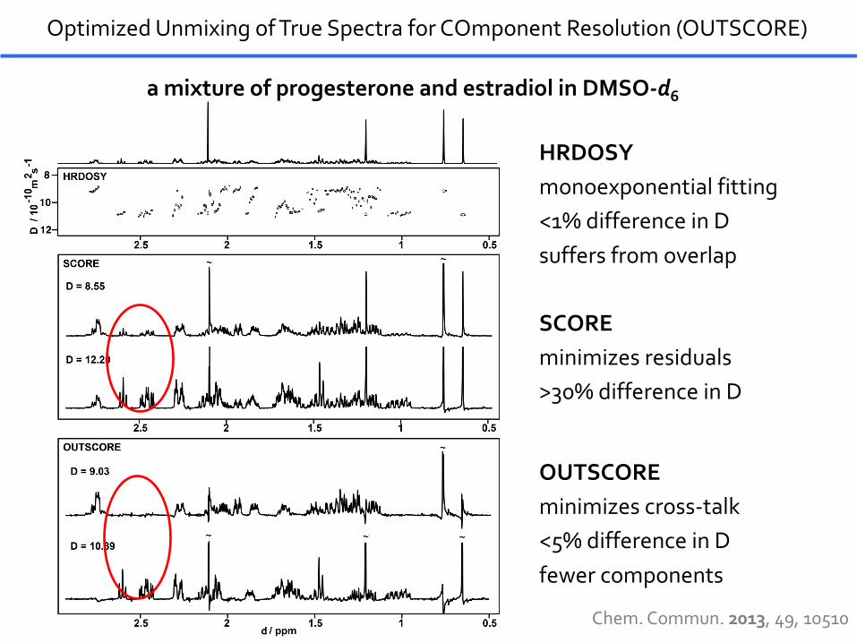
Optimized Unmixing of True Spectra for COmponent Resolution (OUTSCORE)
OUTSCOREminimizes cross-talk<5% difference in Dfewer components
SCOREminimizes residuals>30% difference in D
HRDOSYmonoexponential fitting<1% difference in Dsuffers from overlap
a mixture of progesterone and estradiol in DMSO-d6
Chem. Commun. 2013, 49, 10510
signal overlap in DOSY processing
HR-DOSY
processing
avoid overlap
Chemical shift
multivariate analysis
D= Lower
D= Higher
Chemical shiftChemical shift
multi-exponential
mono-exponential
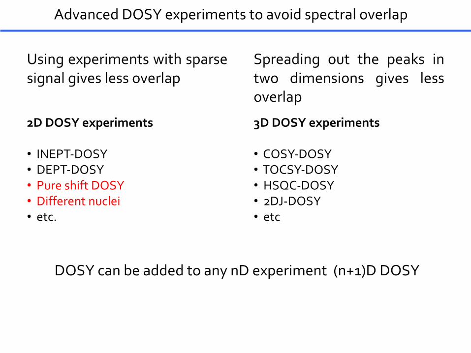
DOSY can be added to any nD experiment (n+1)D DOSY
Advanced DOSY experiments to avoid spectral overlap
Spreading out the peaks intwo dimensions gives lessoverlap
Using experiments with sparsesignal gives less overlap
2D DOSY experiments
• INEPT-DOSY• DEPT-DOSY• Pure shift DOSY• Different nuclei• etc.
3D DOSY experiments
• COSY-DOSY• TOCSY-DOSY• HSQC-DOSY• 2DJ-DOSY• etc
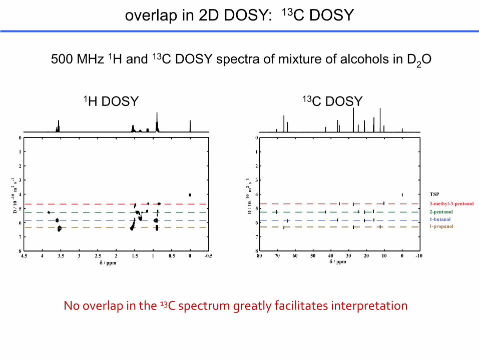
500 MHz 1H and 13C DOSY spectra of mixture of alcohols in D2O
overlap in 2D DOSY: 13C DOSY
No overlap in the 13C spectrum greatly facilitates interpretation
1H DOSY 13C DOSY
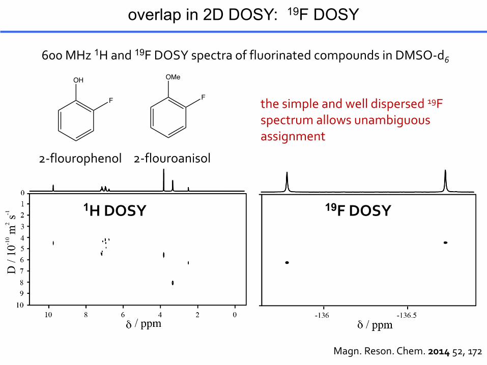
600 MHz 1H and 19F DOSY spectra of fluorinated compounds in DMSO-d6
overlap in 2D DOSY: 19F DOSY
the simple and well dispersed 19F spectrum allows unambiguous assignment
OH
F
OMe
F
2-flourophenol 2-flouroanisol
1H DOSY 19F DOSY
Magn. Reson. Chem. 2014 52, 172
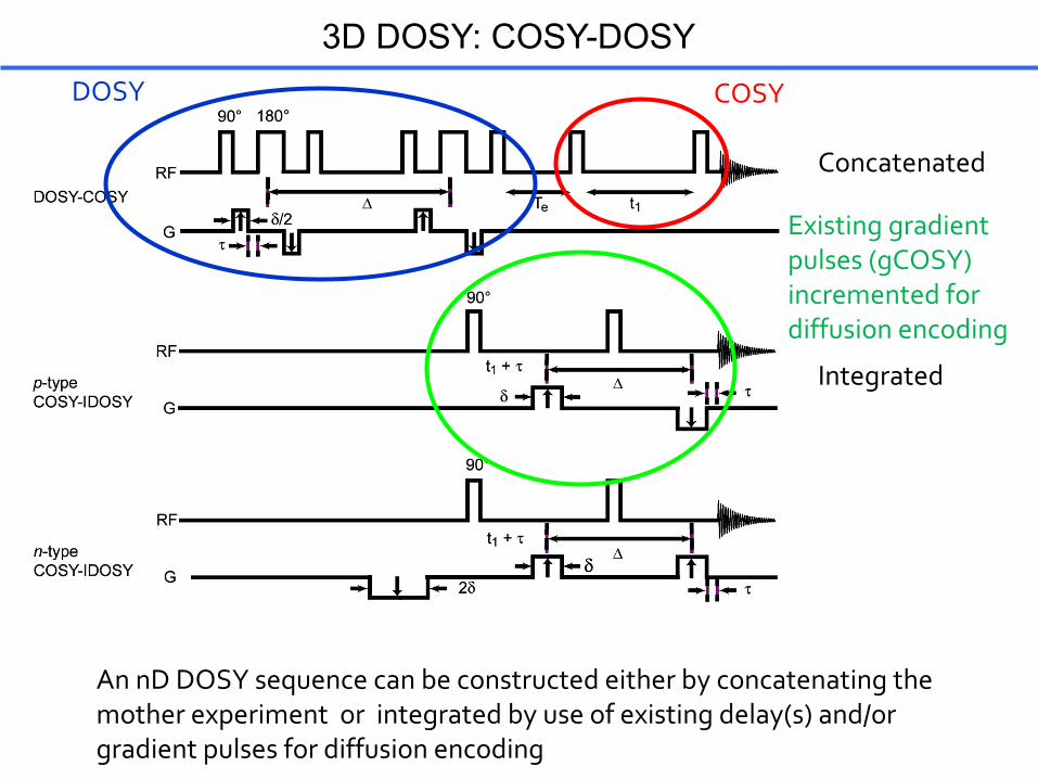
An nD DOSY sequence can be constructed either by concatenating the mother experiment or integrated by use of existing delay(s) and/or gradient pulses for diffusion encoding
3D DOSY: COSY-DOSY
Concatenated
COSYDOSY
Integrated
Existing gradient pulses (gCOSY) incremented for diffusion encoding
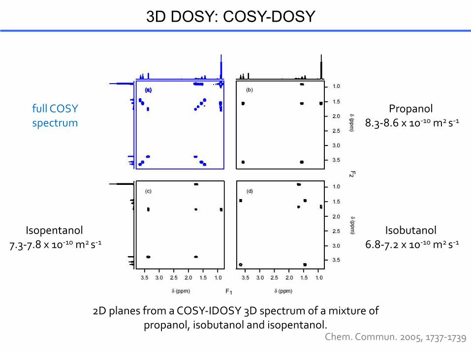
Propanol8.3-8.6 х 10-10 m2 s-1
Isobutanol6.8-7.2 х 10-10 m2 s-1
Isopentanol7.3-7.8 х 10-10 m2 s-1
2D planes from a COSY-IDOSY 3D spectrum of a mixture of propanol, isobutanol and isopentanol.
full COSYspectrum
Chem. Commun. 2005, 1737-1739
3D DOSY: COSY-DOSY
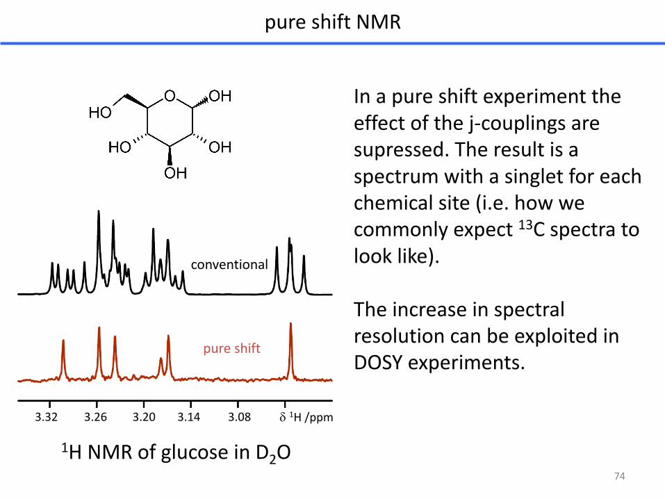
pureshiftNMR
1HNMRofglucoseinD2O
pureshift
conventional
Inapureshiftexperimenttheeffectofthej-couplingsaresupressed.Theresultisaspectrumwithasingletforeachchemicalsite(i.e.howwecommonlyexpect13Cspectratolooklike).
TheincreaseinspectralresolutioncanbeexploitedinDOSYexperiments.
d 1H/ppm3.26 3.143.20 3.083.32
74
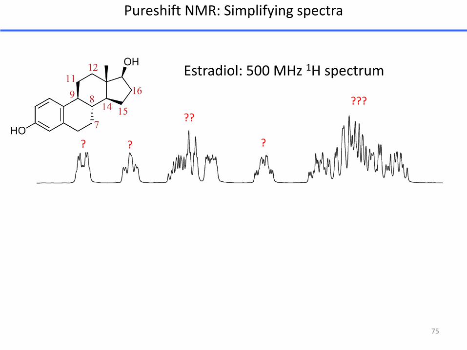
Pureshift NMR:Simplifyingspectra
Angew.Chem.Int.Ed.2014,53,6990
Estradiol: 500 MHz 1H spectrum
?
?????
??
75
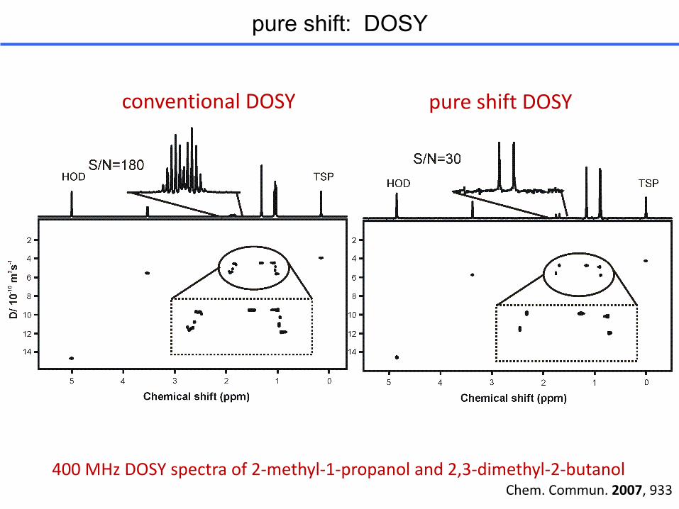
pure shift: DOSY
400MHzDOSYspectraof2-methyl-1-propanoland2,3-dimethyl-2-butanol
pureshiftDOSYconventionalDOSY
Chem.Commun.2007,933
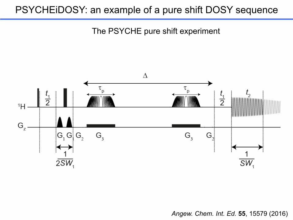
PSYCHEiDOSY: an example of a pure shift DOSY sequence
Angew. Chem. Int. Ed. 55, 15579 (2016)
The PSYCHE pure shift experiment

PSYCHEiDOSY: an example of a pure shift DOSY sequence
Diffusion encoding gradients
Variable diffusion delay
Angew. Chem. Int. Ed. 55, 15579 (2016)
The PSYCHE pure shift experimentcan easily be adapted for diffusion encoding
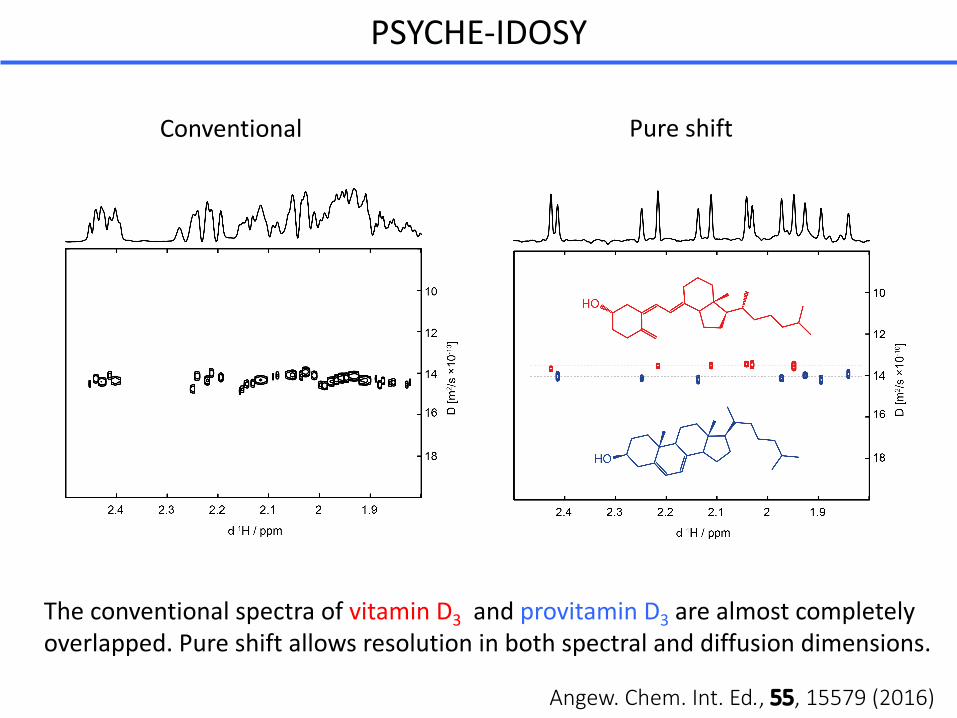
TheconventionalspectraofvitaminD3 andprovitamin D3 arealmostcompletelyoverlapped.Pureshiftallowsresolutioninbothspectralanddiffusiondimensions.
PSYCHE-IDOSY
PureshiftConventional
Angew.Chem.Int.Ed.,55,15579(2016)
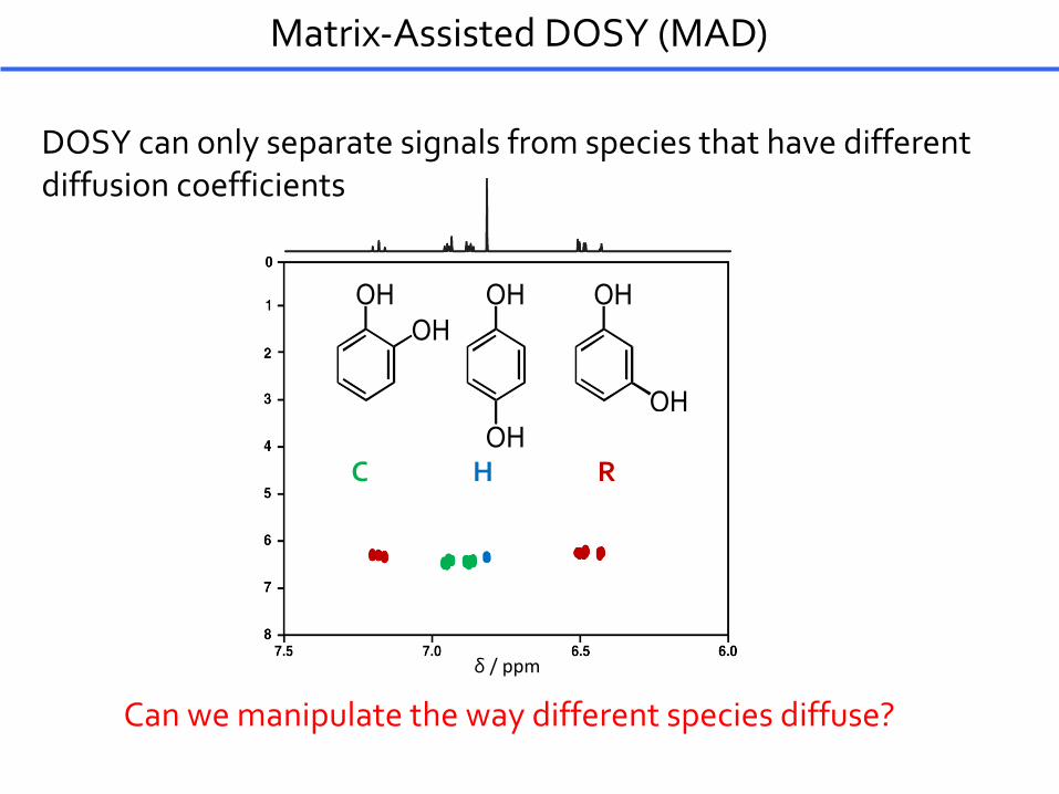
Matrix-Assisted DOSY (MAD)
DOSY can only separate signals from species that have different diffusion coefficients
δ /ppm
OH
OH
OHOH
OH
OH
C H R
Can we manipulate the way different species diffuse?
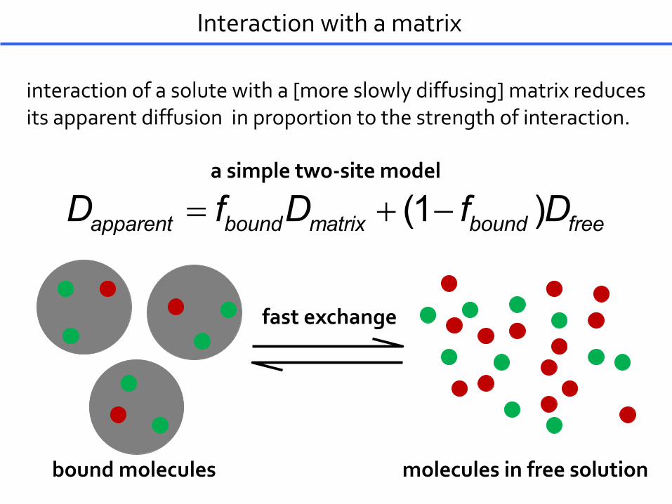
Interaction with a matrix
interaction of a solute with a [more slowly diffusing] matrix reduces its apparent diffusion in proportion to the strength of interaction.
= + -(1 )apparent bound matrix bound freeD f D f Da simple two-site model
bound molecules molecules in free solution
fast exchange
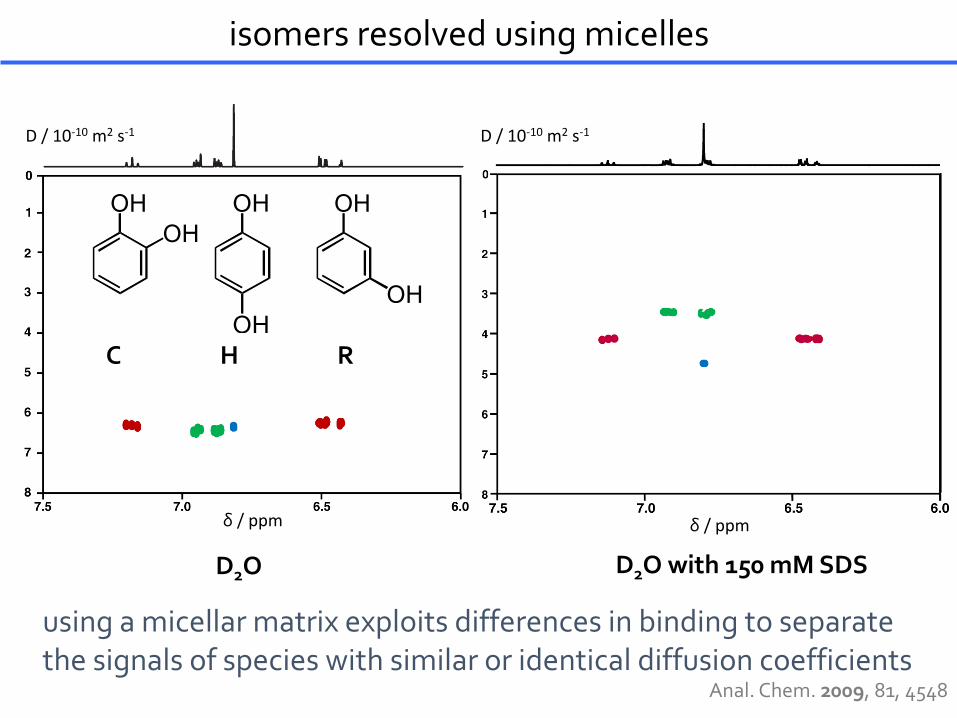
isomers resolved using micelles
using a micellar matrix exploits differences in binding to separate the signals of species with similar or identical diffusion coefficients
Anal. Chem. 2009, 81, 4548
D2O with 150 mM SDS
D /10-10 m2 s-1
δ /ppm
D2O
D /10-10 m2 s-1
δ /ppm
OH
OH
OHOH
OH
OH
C H R
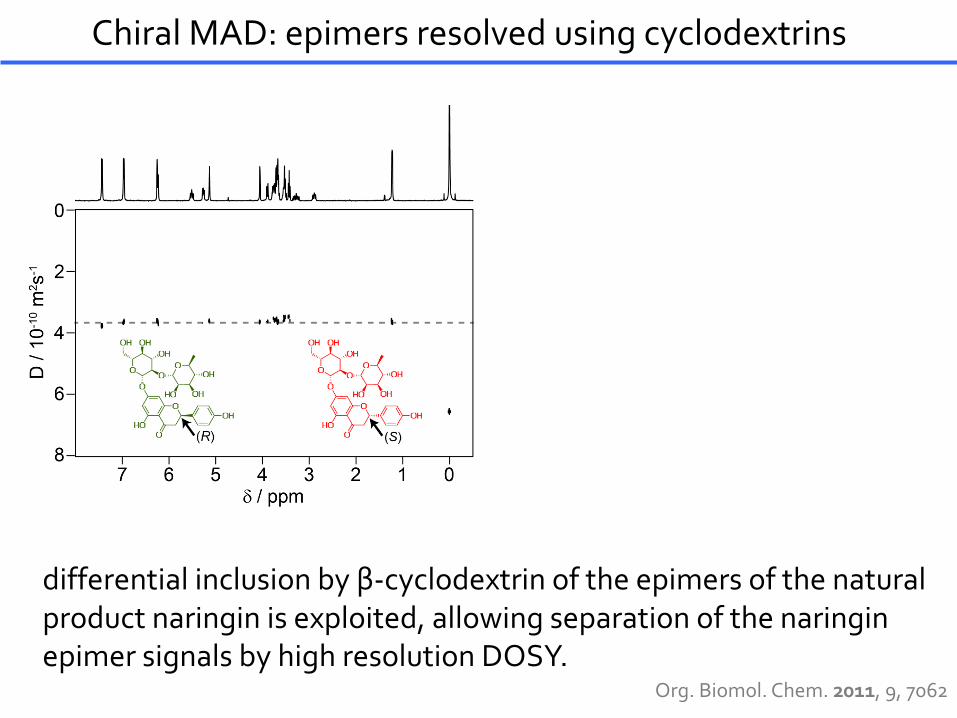
Chiral MAD: epimers resolved using cyclodextrins
differential inclusion by β-cyclodextrin of the epimers of the natural product naringin is exploited, allowing separation of the naringinepimer signals by high resolution DOSY.
Org. Biomol. Chem. 2011, 9, 7062
with cyclodextrin

Lanthanide shift reagents
an “impossible” mixture of hexane, hexanol and hexanal.
adding Eu(fod)3resolves the signals in both dimensions. The signals from hexane, hexanal andhexanol can now be identified
Chem. Commun. 2011, 47, 7063

Diffusion NMR: today’s programme
9.00-9.50 Introduction and Theory
9.50-10.10 Break
10:10-11.00 Acquisition, Analysis and Practicalities
11.00-11.30 Questions and Answers
11.30-14.00 Lunch
14.00-14.50 Advanced experiments
14.50-15.00 Break
15.00-15.50 Introduction to the GNAT Processing software
15.50-16.00 Break
16.00-17.00 Hands on analysis using GNAT, with your own (or provided) data.
17.00-17.30 Conclusion and open discussion

GeneralNMRAnalysisToolbox(GNAT)
87
SupersedestheDOSYToolboxasamoregeneralsoftwarepackage.
Focusedonarrayedexperiments:diffusionrelaxationtimeseries…
RunsunderMatlab 2017aorhigherCompiledversionsforWindows,MacandLinux
LicensedundertheGPLlicence,i.e.freeandopen-source

GeneralNMRAnalysisToolbox(GNAT)
88
Downloadfromourwebsite:http://nmr.chemistry.manchester.ac.uk/
MainWindowoftheGraphicalUserInterface

GeneralNMRAnalysisToolbox(GNAT)
89
Downloadfromourwebsite:http://nmr.chemistry.manchester.ac.uk/
Livedemonstration

Diffusion NMR: today’s programme
9.00-9.50 Introduction and Theory
9.50-10.10 Break
10:10-11.00 Acquisition, Analysis and Practicalities
11.00-11.30 Questions and Answers
11.30-14.00 Lunch
14.00-14.50 Advanced experiments
14.50-15.00 Break
15.00-15.50 Introduction to the GNAT Processing software
15.50-16.00 Break
16.00-17.00 Hands on analysis using GNAT, with your own (or provided) data.
17.00-17.30 Conclusion and open discussion
GeneralNMRAnalysisToolbox(GNAT)
92
Downloadfromourwebsite:http://nmr.chemistry.manchester.ac.uk/
Ifyoudon’thaveyourowndatawe
willprovideexampledatasets

How far does a molecule move by diffusion
The root-mean-square displacement, x, due to diffusion is given by:
𝑥" = 𝛼𝐷𝑡
Where D is the diffusion coefficient, t is time and a is a constant depending on dimensionality; a is 2, 4 or 6 for 1, 2 or 3 dimensional diffusion.
In water at 25°C, D is approximately 2×10⁻⁹ m2 s-1. In 1 minute the average displacement of a water molecule is:
x = 0.6 mm
𝑥 = 6×2×10.C×60�
Diffusion NMR: today’s programme
9.00-9.50 Introduction and Theory
9.50-10.10 Break
10:10-11.00 Acquisition, Analysis and Practicalities
11.00-11.30 Questions and Answers
11.30-14.00 Lunch
14.00-14.50 Advanced experiments
14.50-15.00 Break
15.00-15.50 Introduction to the GNAT Processing software
15.50-16.00 Break
16.00-17.00 Hands on analysis using GNAT, with your own (or provided) data.
17.00-17.30 Conclusion and open discussion

9 8 7 6 5 4 3 2 1 ppm
789 ppm
(with triple presaturation of water and ethanol)
J. Agric. Food Chem. 52, 3736 (2004)
Port Wine: 500 MHz proton spectrum

![Analytical Methods Diffusion NMR Spectroscopy in ... · Diffusion NMR Spectroscopy in Supramolecular and Combinatorial Chemistry: ... copy [22] laid the ... homogeneous system the](https://img.dokumen.tips/doc/110x75/5afef5407f8b9a444f8f87da/analytical-methods-diffusion-nmr-spectroscopy-in-nmr-spectroscopy-in-supramolecular.jpg)


![Analytical Methods Diffusion NMR Spectroscopy in ...NMR methods was realised in the early days of NMR spectroscopy.[4] The most practical pulse sequence for meas-uring diffusion coefficients](https://img.dokumen.tips/doc/110x75/5e8766a7c364ec7447604f65/analytical-methods-diffusion-nmr-spectroscopy-in-nmr-methods-was-realised-in.jpg)