Introduction to Differential Equations and Fourier Series:

Math 110 Section Notes

Christopher Eur

May 20, 2015

As the second time course assistant for this course, I have decided to go a bit furtherthan making section notes for Math 110 Spring 2015 and expound my understanding ofthe course material into a lengthy document, rather than series of disparate collection ofnotes. I do not claim in anyway that the content of this document is correct nor elegant,but I have tried to bring a more modern flavor to the material when possible, as Holland’sApplied Analysis by Hilbert Space Method does not do so. Please email any errata you mayfind to ceur@college.harvard.edu.

Note for students: This is intended to supplement and in no way substitute the lec-ture outlines for Math 110. The primary purpose is to review the material and occasionallyprovide different perspectives. My hope is that it will help provide a big picture to thematerial being covered in the lectures. Enjoy!

1

Contents

1 Preliminaries 31.1 Linear Algebra Review . . . . . . . . . . . . . . . . . . . . . . . . . . . . . . 31.2 Vector Spaces of Functions . . . . . . . . . . . . . . . . . . . . . . . . . . . 51.3 Definition of Differential Equations . . . . . . . . . . . . . . . . . . . . . . . 61.4 Definition of Linear ODE . . . . . . . . . . . . . . . . . . . . . . . . . . . . 8

2 First Order Linear ODE 92.1 Integrating Factor . . . . . . . . . . . . . . . . . . . . . . . . . . . . . . . . 92.2 Variation of Parameters . . . . . . . . . . . . . . . . . . . . . . . . . . . . . 102.3 Green’s Function . . . . . . . . . . . . . . . . . . . . . . . . . . . . . . . . . 102.4 Power Series . . . . . . . . . . . . . . . . . . . . . . . . . . . . . . . . . . . . 11

3 Preliminaries for Second Order ODE 123.1 The Wronskian and Abel . . . . . . . . . . . . . . . . . . . . . . . . . . . . 123.2 General Facts on the Kernel of Second Order ODE . . . . . . . . . . . . . . 13

4 Second Order Homogeneous ODE 144.1 Constant a, b, c Case . . . . . . . . . . . . . . . . . . . . . . . . . . . . . . . 144.2 Laplace Transforms . . . . . . . . . . . . . . . . . . . . . . . . . . . . . . . . 144.3 Green’s function for 2nd order ODE . . . . . . . . . . . . . . . . . . . . . . 15

5 Hilbert Spaces 165.1 Metric Space Preliminaries . . . . . . . . . . . . . . . . . . . . . . . . . . . 165.2 On convergence of sequence of functions . . . . . . . . . . . . . . . . . . . . 205.3 Interlude: Lebesgue Integral Basics . . . . . . . . . . . . . . . . . . . . . . . 215.4 L2 space . . . . . . . . . . . . . . . . . . . . . . . . . . . . . . . . . . . . . . 215.5 An aside: on convergence of sequence of functions . . . . . . . . . . . . . . . 21

6 Sturm-Liouville Theory 226.1 Classical Fourier Series . . . . . . . . . . . . . . . . . . . . . . . . . . . . . . 226.2 Isoperimetric inequality . . . . . . . . . . . . . . . . . . . . . . . . . . . . . 23

2

CHAPTER 1

Preliminaries

In this chapter, we review and introduce the linear algebraic language that we will be usingthrough out this course. We finish with the definition of (linear) differential equations.

1.1 Linear Algebra Review

We assume that the reader is familiar with basic linear algebra. The following sectioncan be skipped for anyone with sufficient linear algebra background. A good reference isAxler’s Linear Algebra Done Right Ch. 1,2,3,5 and Artin’s Algebra Ch. 1,3,4.

Definition 1.1.1. A field is a set where one can add, subtract, multiply, and divide (exceptby 0) elements.

Example 1.1.2. The set of rational numbers Q, real numbers R, and the complex numbersC are all examples of a field. The set of integers Z is not a field because division is closedin Z. The set of natural numbers N is also not a field because it doesn’t include negativenumbers (i.e. 5− 8 for example doesn’t exists in N).

In this class, a field will be either R or C unless stated otherwise.

Definition 1.1.3. A vector space V over a field F is a set V with maps V ×V +→ V andF× V ·→ V (called vector addition and scalar multiplication respectively) such that:

1. v + w = w + v ∀v, w ∈ V

2. ∃ element denoted 0 ∈ V such that 0 + v = v = v + 0 ∀v ∈ V

3. ∀v ∈ V ∃w ∈ V such that v + w = w + v = 0

4. 1 · v = v and (ab) · v = a · (b · v) ∀a, b ∈ F, v ∈ V

5. a(v + w) = av + aw and (a+ b)v = av + bv ∀a, b ∈ F, v, w ∈ V

3

Definition 1.1.4 (Concise definition). A vector space V over a field F (i.e. R or C) is a

set V with a binary operation V × V +→ V and a field action F × V ·→ V such that 〈V,+〉is an Abelian group and distributivity holds.

Example 1.1.5. A field F is a vector space over itself. Rn with the usual definition of addi-tion and scalar multiplication is a vector space over R. PC := {polynomials with coefficients in C}is a vector space over C.

Definition 1.1.6. Let V be a vector space. A subset U of V that is also a vector space isa subspace of V . Given U ⊂ V , in order to show that U is a subspace we need check:

1. closed under addition: u, v ∈ U ⇒ u+ v ∈ U

2. closed under scalar multiplication: a ∈ F and u ∈ U ⇒ au ∈ U

Example 1.1.7. V := {(x, y, 0) ∈ R3 | x, y ∈ R} is a vector subspace of R3. PCn , the set

of polynomials of degree ≤ n, is a vector subspace of PC.

Exercise 1.1.A (Non-examples). Give an example of a subset of R2 that is not a vectorsubspace and: (i) satisfies condition 1. but not 2. (in Definition 1.1.6.); (ii) satisfies 2.but not 1.

Solution. (i) Z2 ⊂ R2 is not a subspace (satisfies 1. but not 2.). (ii) (x-axis)∪(y-axis)⊂ R2

is not a subspace (satisfies 2. but not 1.)

Definition 1.1.8. Let V,W be vector spaces over F. A function T : V → W is a linearmap if T (v+v′) = Tv+Tv′ and T (av) = a(Tv) for any v, v′ ∈ V and a ∈ F. Equivalently,T is linear if T (av + v′) = a(Tv) + Tv′ for any v, v′ ∈ V and a ∈ F.

Definition 1.1.9. Let T : V → W be a linear map. The kernel of T is kerT := {v ∈V | Tv = 0} and the image of T is Im(T ) := {w ∈W | w = Tv for some v ∈ V }.

Exercise 1.1.B. Prove that kerT ⊂ V is a vector subspace, and Im(T ) ⊂ W is a vectorsubspace.

Solution) For kerT , note that if v, w ∈ kerT then T (v + w) = Tv + Tw = 0 + 0 = 0 andT (av) = a(Tv) = a0 = 0. For Im(T ), if w,w′ ∈ Im(T ) then there exists v, v′ ∈ V such thatTv = w, Tv′ = w′, and thus w + w′ = Tv + Tv′ = T (v + v′) and aw = a(Tv) = T (av).

Definition 1.1.10. A basis for a vector space V (over F) is an ordered list of vectorsB = (v1, . . . , vn) such that every element v ∈ V can be uniquely written as v = a1v1 +· · ·+ anvn for some (a1, . . . , an) ∈ Fn. In other words, a basis for V establishes a bijectivecorrespondence between Fn and V via (a1, . . . , an)↔ a1v1 + · · · anvn.

Given a basis B for V , let’s denote by M(v) the vector in Fn that corresponds to v via thebijection in the definition given above.

4

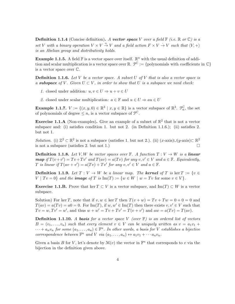
Example 1.1.11. Consider PR2 , the set of polynomials of degree ≤ 2 with real coefficients.

One can see that (1, x, x2) is a basis for PR2 , and with this basis 1 + x2 corresponds to the

vector

101

. Moreover, if one could also use (1, 1 +x, 1 +x+x2) as the basis, in which case

1 + x2 corresponds to

1−11

.

Proposition 1.1.12. Let (v1, . . . , vn), (w1, . . . , wm) be the bases for V,W respectively, andlet T : V → W be a linear map such that Tvj = a1jw1 + · · · + amjwm for j = 1, . . . , n.Then

M(Tv) = [A]M(v)

where [A] is the matrix

[A] =

v1 . . . vj . . . vnw1...wm

a11 . . . a1j . . . a1n...

......

am1 . . . amj . . . amn

Example 1.1.13. Let’s consider the map d : PR

3 → PR2 given by differentiation (which is

known to be linear). With bases (1, x, x2) and (1, x) respectively, the matrix [A] in this

case is

[0 1 00 0 2

]. Sanity check: [A]

101

=

[02

]and (1 + x2)′ = 2x.

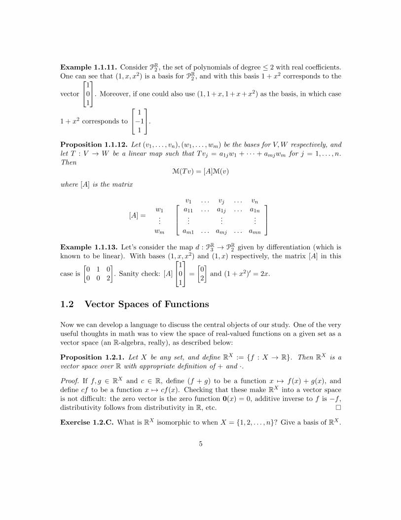
1.2 Vector Spaces of Functions

Now we can develop a language to discuss the central objects of our study. One of the veryuseful thoughts in math was to view the space of real-valued functions on a given set as avector space (an R-algebra, really), as described below:

Proposition 1.2.1. Let X be any set, and define RX := {f : X → R}. Then RX is avector space over R with appropriate definition of + and ·.

Proof. If f, g ∈ RX and c ∈ R, define (f + g) to be a function x 7→ f(x) + g(x), anddefine cf to be a function x 7→ cf(x). Checking that these make RX into a vector spaceis not difficult: the zero vector is the zero function 0(x) = 0, additive inverse to f is −f ,distributivity follows from distributivity in R, etc.

Exercise 1.2.C. What is RX isomorphic to when X = {1, 2, . . . , n}? Give a basis of RX .

5

Solution. RX ' Rn above. RX is the set of all the functions from X to R, but givinga function from X = {1, . . . , n} to R is same thing as picking n-tuple of real numbersa1, . . . , an. That is, if the function f ∈ RX , then we can identify f with the n-tuple(f(1), f(2), . . . , f(n)). A natural basis to pick is (f1, . . . , fn), where fi is a function thathas value 1 at i and 0 otherwise.

Remark 1.2.2. RR is the “set of all single-variable real-valued functions”

Much of real analysis is concerned with “nice” subspaces of RR. Here are some importantexamples:

Definition 1.2.3. Define C(R) := {f : R → R | f is continuous}, Ck(R) := {f :R→ R | f (k) (the k-th derivative) is continuous}, and Pn := {polynomials of degree ≤ n}.Moreover, define the set of smooth functions to be C∞(R) := {f : R → R | f (k) ∈C(R) ∀k ∈ N} (i.e. infinitely differentiable functions).

Proposition 1.2.4. C(R), Ck(R), and Pn are linear subspace of RR. In fact, they are alsosubspaces of each other in the order Pn ⊂ Ck(R) ⊂ C(R).

Proof) From calculus we know that sums and scalar multiples of continuous functionsare continuous. Moreover, differentiation is linear ((cf +g)′ = cf ′+g′), so sums and scalarmultiples of Ck(R) functions are also Ck(R). Lastly, polynomials are closed under sumand scalar multiplication. So, Pn, Ck(R), C(R) are all vector subspaces of RR. Moreover,differentiable implies continuous, and polynomials are infinitely differentiable, and thusPn ⊂ Ck(R) ⊂ C(R).

Remark 1.2.5. The set of smooth functions is strictly bigger than the set of real-analyticfunctions (i.e. functions that can be written faithfully as a Taylor series). An example ofsmooth function that is not analytic is one defined as :f(x) = 0 for x ≤ 0 and f(x) = e−1/x

2

for x > 0.

1.3 Definition of Differential Equations

Definition 1.3.1. A differential equation is an equation containing one or more deriva-tives of the function in consideration. The order of the differential equation is the highestpower of derivative that appears in it. To solve the differential equation means findinga function f that satisfies a given differential equation.

Example 1.3.2. Differential equations with appropriate functions under consideration:

1. f ′(x) = ex + xex (solution: f(x) = xex)

2. f ′′(x)− f ′(x) = ex (solution: same as above)

6

3. (∂f∂x )(∂f∂y )− f(x, y) = 0 (solution: f(x, y) = xy)

Definition 1.3.3. An ordinary differential equation (ODE) is differential equationwhere the function under consideration is a single-variable function f : R → R. In moreconcrete terms, an ordinary differential equation of order k is a differential equationof the form:

[an expression in f(x), f ′(x), . . . , f (k)(x)] = h(x), h(x) some function of x

Note that 1. and 2. (but not 3.) in Example 1.1.2 are ordinary differential equations.Example 3. is called a partial differential equation (PDE). It is assumed that youhave worked with ODEs before, but in case you have not, the following is essentially allthe ODE you need to know for the course:

Exercise 1.3.D. (Conventionally, we write y in place of f(x).) Solve the following ordinarydifferential equations:

1. y′ = 1/x

2. y′ = ky (alt. y′/y = k)

3. y′/y = f(x) where F ′(x) = f(x) for some function F .

Solution.1. Rewrite as dy/dx = 1/x so that dy = 1

xdx, and integrate both sides to get y = ln |x|+C;most of the time we assume x > 0 so lnx is fine.2. Again, rewriting y′/y = (dy/dx)/y = (dy/y)/dx, we get 1

ydy = kdx, and Integrating,

we get ln |y| = kx+C, so |y| = ekx+C , i.e. y = ±eCekx, and absorbing ± into the constantterm, we get y = Cekx.3. We solve exactly as we did for 2., and get y = CeF (x).

Definition 1.3.4. Suppose we are given an ODE, say:

[expression in f, f ′, . . . , f (k)(x)] = h(x)

Then we can consider the map f 7→ [expression in f, f ′, . . . , f (k)] as a map F : Ck(R) →RR. We call such F a differential expression.

Remark 1.3.5. So the study of ODE can be rephrased as: “Given F : Ck(R)→ RR andh ∈ RR, can we find f ∈ Ck(R) such that F (f) = h? and how so?”

7

1.4 Definition of Linear ODE

We now define what is the central object of our course:

Definition 1.4.1. An ODE whose differential expression F is a linear map is called alinear ODE. Equivalently, a linear ODE of order k is an ODE of the form:

a0(x)f(x) + a1(x)f ′(x) + · · ·+ ak(x)f (k)(x) = h(x), (ak(x) 6= 0)

When ODE is linear, we call F differential operator and denote it as `.

We will only study linear ODEs in this course. Our aim is to figure out how to exploitthe fact that F : Ck(R) → RR is a linear map of two vector spaces, since vector spacesand linear maps are rather well-understood objects. From this point on, an “ODE”means “linear ODE” unless otherwise stated .

Here are two immediate consequences where our linear algebraic view pays off:

Proposition 1.4.2. A linear ODE is called homogeneous if the h(x) in the equation iszero. If f, g are solutions to a homogeneous ODE, then so are any linear combinations off, g.

Proof) That f, g are solutions to the homogeneous ODE means that f, g ∈ ker(`), where` is the differential operator of the homogeneous ODE. But ker(`) is a subspace.

Proposition 1.4.3. Let `(y) = h(x) be a linear ODE, yp a particular solution. Thenyp + ker(`) is the general solution. (In fact, previous proposition is just a special case ofthis).

Exercise 1.4.E. Prove the above proposition

Remark 1.4.4. Suppose `(y) = h(x) where h(x) ∈ Pn, and we want a polynomial solution(of degree < n). Then we can restrict ` to ` : Pn → Pn, a linear map of finite dimensionalvector spaces, which we understand very well, and so the problem becomes very easy withlinear algebra.

Now we are ready to study linear ODEs.

8

CHAPTER 2

First Order Linear ODE

First order linear ODEs are of the form a(x)y′(x) + b(x)y(x) = h(x) for some functionsa, b, h. In other words, the differential operator is `(y) = ay′ + by. Luckily, for first ordercase the kernel is easy to find:

Proposition 2.0.5. The kernel of the differential operator `(y) = ay′+by is a 1-dimensional

space spanned by e∫−b/a.

Proof) Solving for ay′ + by = 0, we have y′/y = −b/a and hence Ce∫−b/a.

We have four main methods of solving first order linear ODEs: integrating factor, variationof parameters, Green’s function, and power series. The first three are closely related.

2.1 Integrating Factor

Let ay′ + by = h be given. Note that if the LHS is of the form (µy)′ for some µ(x), thedifferential equations is easy to solve. One way to make ay′ + by into such form is bymultiplying by an appropriate function µ. That is, if we multiply µ to the expression, weget aµy′ + bµy =

Definition 2.1.1. Let ay′ + by = h be given; equivalently, y′ + bay = h

a . An integrating

factor µ(x) is a function such that (µ(x)y)′ = µ(x)(y′ + bay).

Proposition 2.1.2. If µ is the integrating factor for ay′+ by = c, then the solution to thedifferential equation is

y(x) =1

µ(x)

∫ x

x0

h(t)µ(t)

a(t)dt

And in fact, µ(x) = exp(∫badx)

Proof) Lecture.

9

Example 2.1.3. Crofton’s method: Suppose we want to express some quantity y asfunction of x, and suppose it is reasonable to believe that y(x) is differentiable. Thentranslate the problem into a ODE problem and then solve for y(x).

2.2 Variation of Parameters

Proposition 2.2.1. The kernel of the map ` : y 7→ ay′ + by is one dimensional. In fact,it is spanned by f(x) = exp(−

∫badx).

Proof) Lecture

Exercise 2.2.A. Note that that (integrating factor)−1 =(kernel of `). Why is it so? Usethis to motivate the method of variation of parameters stated below.

Proposition 2.2.2. Let `(y) = ay′ + by and f ∈ ker(`). Then the variation of param-eter method, which is setting y = gf , yields the solution to `(y) = h as:

y(x) = f(x)

∫ x

x0

h(t)

a(t)f(t)dt

Proof) Lecture

In sum, either through integrating factors or variation of parameters, we conclude:

Theorem 2.2.3. The solution to ay′ + by = h with initial condition y(x0) = 0 is

y(x) = exp

(∫− badx

)∫ x

x0

h(t)

a(t) exp(− badt)

dt

2.3 Green’s Function

Here we develop a language to state Theorem 2.1.7. in a slightly different way. We willsee the benefit of doing this later in the course.

Definition 2.3.1. The Heaviside function H(x) is defined as:

H(x) =

{0 if x < 01 if x ≥ 0

and the Dirac delta function δ(x) is defined as H ′(x).

Remark 2.3.2. Strictly speaking, δ(x) is what we call a “generalized function,” or a“distribution.” For our purposes, we just treat δ(x) as H ′(x).

10

We now list some properties of these two functions:

Proposition 2.3.3. Let H(x) and δ(x) be defined as above, and let a < b:

1. A function that is 1 on (a, b] and 0 elsewhere is H(b− t)−H(a− t)

2.∫ ba f(x)δ(x− t)dx = f(t) if t ∈ (a, b) and 0 otherwise.

3. f(x)δ(x− t) = f(t)δ(x− t)

Proof) Lecture

Definition 2.3.4. Let `(y) = ay′ + by with the condition y(x0) = 0, and f ∈ ker(`). Thenthe Green’s function G(x, t) for ` is defined as:

G(x, t) =f(x)

a(t)f(t)[H(x− t)−H(x0 − t)]

Theorem 2.3.5. (cf. Theorem 2.2.3) Suppose G(x, t) is the Green’s function for `(y) =ay′ + by with y(x0) = 0. Then,

1. y(x) =∫∞−∞G(x, t)h(t)dt is the solution to the differential equation.

2. G(x, t) regarded as a function of x with t fixed satisfies `(G(x, t)) = δ(x− t).

Remark 2.3.6. Let a differential expression `(y) = ay′ + by and a condition y(x0) = 0 begiven, and let G(x, t) be the Green’s function. Noting that V := {f ∈ C1(R) | f(x0) = 0}is a subspace of C1(R), we may restrict ` to V ; i.e. we have ` : V → RR. Now defineW = {h ∈ RR |

∫∞−∞G(x, t)h(t)dt ∈ C1(R)}. Then, a linear transformation `−1 : W → V

given by h(x) 7→∫∞−∞G(x, t)h(t)dt is the inverse of `.

2.4 Power Series

Power series approach does not provide much interesting results in first order linear ODEs.It can be summed up as: write y = y0 +y1x+y2x

2 + · · · and using the differential equationsolve for the coefficients y0, y1, . . .. We thus discuss this method in more depth in the nextchapter.

11

CHAPTER 3

Preliminaries for Second Order ODE

3.1 The Wronskian and Abel

The kernel of second (or higher) order differential operator is no longer guaranteed to beone-dimensional (nor is it as easy to compute as in the first order case). So, we first needto develop a tool to test whether a set of functions are linearly independent.

Observation 3.1.1. Recall: Let {f1, f2, . . . , fk} ⊂ RR be linearly independent set of func-tions. If a1f1 + ·anfn = 0 for ai ∈ R (i = 1, . . . , n), then a1 = a2 = · · · = an = 0.

Definition 3.1.2. Let f1, f2, . . . , fn ∈ Cn−1(R). The Wronskian of f1, . . . , fn, denotedW (f1, . . . , fn), is a function of x defined as:

W (f1, . . . , fn) := det

f1 · · · fn...

. . ....

f(n−1)1 · · · f

(n−1)n

Theorem 3.1.3. Let {f1, f2, . . . , fn} ⊂ Cn−1(R) be a set of functions. If they are linearlydependent, then W (f1, . . . , fn) ≡ 0. Equivalently, If W (f1, . . . , fn)(x) 6= 0 for some x,then f1, . . . , fn are linearly independent.

Proof) Lecture

Remark 3.1.4. The converse of the theorem if not true: x2, x|x| are linearly independent,but W (x2, x|x|) ≡ 0.

Remark 3.1.5. Given f1, f2 linearly independent, W (y, f1, f2) = 0 yields a second orderlinear ODE with solutions f1 and f2.

Theorem 3.1.6 (Abel’s Formula). Let f1, f2 be any linearly independent solutions to`(y) = ay′′ + by′ + cy = 0, and let W = W (f1, f2). Then aW ′ + bW = 0, and henceW = C exp(−

∫badx)

Proof) Lecture

12

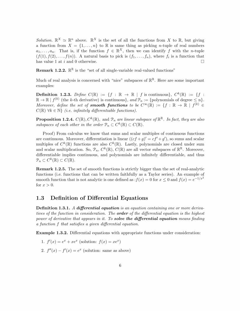
3.2 General Facts on the Kernel of Second Order ODE

Before we discuss the kernel of second order linear ODE, we need an important theorem:

Theorem 3.2.1. Let a linear ODE be given: a(x)y′′+b(x)y′+c(x) = 0, with a(x), b(x), c(x)analytic around x0 and a(x0) 6= 0. Then, for any y0, y1 ∈ R, there exists unique analyticsolution y(x) around x0 such that y(x0) = y0 and y′(x0) = y1.

Proof) Lecture

Corollary 3.2.2. Let `(y) = ay′′ + by′ + c = 0 satisfy the conditions as in the previoustheorem. Then, dim ker(`) = 2

Proof) Lecture

The previous corollary shows that most “normal-looking” second order linear ODEs have2-dimensional kernel. For most cases, we only see a, b, c be polynomials, trigonomet-ric/exponential functions, etc. Hence, unless otherwise stated, for the rest of the sectionassume that all the second order linear ODEs we consider satisfy dim ker(`) = 2.

With such assumption, we can do much much more.

Proposition 3.2.3. Let `(y) = 0 be a second order linear ODE. Then, for any f1, f2 ∈ker(`) linearly independent, W (f1, f2) is the same up to a multiplicative constant. Hence,Wronskian is inherent to `, not particular bases of ker(`)

Proof) Lecture

Proposition 3.2.4. Let `(y) = 0 be second order linear ODE, W (x) be the Wronskian,and suppose f1 ∈ ker(`) is known, then the other linearly independent f2 ∈ ker(`) equals:

f2(x) = f1(x)

∫ x W (t)

(f1(t))2dt

Proof) Lecture

Before moving on, we briefly treat what to do when a(x0) = 0 (i.e. is regular singular).

Proposition 3.2.5 (Method of Frobenius). Suppose we are given y′′+ pxy′+ q

x2y = 0, then

we can try to solve for y of the form y = y0xk +y1x

k+1 + ·. k satisfies the indicial equationk2 + (p0 − 1)k + q0 = 0.

13

CHAPTER 4

Second Order Homogeneous ODE

Here we give methods to find the kernel of a second order differential operator (i.e. how tosolve second order homogeneous ODEs).

4.1 Constant a, b, c Case

Proposition 4.1.1. If given ay′′ + by′ + c = 0 with a, b, c constants, the general solutionis C1e

αx + C2eβx if α, β are two distinct solutions of ar2 + br + c = 0. If α = β, we have

C1eαx + C2xe

αx.

Proof) Lecture

4.2 Laplace Transforms

Definition 4.2.1. The Laplace Transform is the linear operator L defined on the spaceof integrable functions that does not grow faster than any exponential, defined by:

L(f) = f(s) =

∫ ∞0

f(x)e−sxdx

Remark 4.2.2. Often the problem becomes easier by applying Laplace Transform on thedifferential equation a(x)y′′(x) + b(x)y′(x) + c(x) = h(x) to find what y(s) has to be, andthen we do the inverse of the Laplace transform to find y(x).

Proposition 4.2.3. Let y 7→ y be the Laplace transform. Then:

1. If y(x) = c (constant), then y(s) = cs

2. y′(s) = sy(s)− y(0)

3. y′′(s) = s2y(s)− sy(0)− y′(0)

14

Proof) Lecture

Corollary 4.2.4. Suppose we are given ay′′ + by′ + c = 0 (a, b, c constants). Then thesolution y satisfies:

y(s) =ay(0)s+ by(0) + ay′(0)

as2 + bs+ c

Proof) Lecture

Proposition 4.2.5. We establish some Laplace Transforms:

1. If y(x) = eαx, then y(s) = 1s−α .

2. If y(x) = xneαx, then y(s) = n!(s−α)n+1 .

3. If y(x) = e(α+iω)x, then y(s) = 1s−α−iω = s−α+iω

(s−α)2+ω2 .

4. If y(x) = eαx cosωx, then y(s) = s−α(s−α)2+ω2 ,

if y(x) = eαx sinωx, then y(s) = ω(s−α)2+ω2 .

4.3 Green’s function for 2nd order ODE

15

CHAPTER 5

Hilbert Spaces

We now come to introductory functional analysis. In this course, we will exclusively focuson Fourier series, both the classical sine/cosines and the more general Sturm-Liouvilletheory.

In this chapter, we introduce the fundamental object underlying the study of Fourierseries: the Hilbert space. We first begin with the brief treatment of metric space topologythat will set the language throughout our discussion. We will then specialize this to thespace of functions, which we are ultimately interested in. In the end, we arrive at L2 space,which is a subspace of functions that is the playing field of our Fourier series analysis.

5.1 Metric Space Preliminaries

We here give a brief treatment of metric space topology that will be useful and/or necessaryfor our forthcoming discussion of Hilbert spaces.

Definition 5.1.1. A metric space is a set X with a distance function, or a metric,d : X ×X → [0,∞) such that:

1. d(x, y) = 0 ⇐⇒ x = y

2. d(x, y) = d(y, x)

3. d(x, z) ≤ d(x, y) + d(y, z)

Example 5.1.2. One easy example is R with the absolute value of the difference as thedistance, i.e. d(x, y) = |x−y|. When we say R, we will always assume R to have this metricunless stated otherwise.

One can generalize this to Rn in many different ways. If x,y ∈ Rn, then one candefine d1(x,y) :=

√(x1 − y1)2 + · · ·+ (xn − yn)2 (this is the usual Euclidean distance), or

d2(x,y) := max(|x1 − y1|, . . . , |xn − yn|) (this is usually called the “infinity norm”). While

16

the two metrics d1, d2 on Rn are different, we will later see that they are equivalent in thatif a sequence {an} ⊂ Rn converges with respect to d1 it also converges with respect of d2,and vice versa.

Once we have a metric space, we can sensibly talk about convergence of a sequence, con-tinuity, Cauchy sequences, and completeness.

Definition 5.1.3. Let X be a metric space with a metric d, and let x1, x2, . . . be a sequencein X. For some x ∈ X, we say that the sequence xn converges to x, or lim

n→∞xn = x, or

xn → x as n→∞, if ∀ε > 0, ∃N s.t. ∀m ≥ N d(xm, x) < ε.

Exercise 5.1.A (Easy). Show that the sequence { 1n}n=1,2,... converges to 0 in R with itsusual metric. Show that the sequence 1,−1, 1,−1, . . . does not converge in R.

Exercise 5.1.B. Prove the claim that if a sequence {an} ⊂ Rn converges in metric d1,then it also converges in metric d2 of Rn, and vice versa. When we say Rn, we will assumed1, or equivalently d2, to be the metric when dealing with convergent sequences.

Definition 5.1.4. Let (X, dX), (Y, dY ) be metric spaces. A function f : X → Y is:

• continuous if for all x0 ∈ X and ε > 0 there exists δ > 0 such that dX(x0, x) < δimplies dY (f(x0), f(x)) < ε.

• uniformly continuous if for all ε > 0 there exists δ > 0 such that dX(x, x′) < δimplies dY (f(x), f(x′)) < ε.

One should confirm that with X = Y = R, the above definition is exactly the ε-δcontinuity definition that one usually sees in an introductory calculus class. Note that thetwo definitions, while looking similar, are actually different. Uniform continuity impliescontinuity, but not conversely.

Exercise 5.1.C. Show that uniform continuity implies continuity. Show that sinx is uni-formly continuous whereas 1/x on x ∈ (0,∞) is continuous but not uniformly continuous.

A great feature of metric spaces is that continuity can be detected by convergent se-quences. More precisely,

Proposition 5.1.5. Let (X, dX), (Y, dY ) be metric spaces. Then f : X → Y is continuousif and only if for every convergent sequence {xn} ⊂ X converging to x ∈ X, the sequence{f(xn)} ⊂ Y is a convergent sequence in Y converging to f(x). In other words,

f is continuous ⇐⇒ for any sequence xn → x in X, f(xn)→ f(x) in Y

Exercise 5.1.D. Prove the above proposition.

17

To test if a given sequence {xn} converges, one must produce x such that xn → x, butproducing such x just by looking at {xn} may sometimes be a difficult task. Is there away to test convergence without explicitly knowing what the sequence converges to? Thisbrings us to the topic of Cauchy sequences and completeness. If we can’t really pick outx that xn may converge to, the next best thing would be to require that the sequence xn“clusters together.” More precisely,

Definition 5.1.6. Let X be a metric space with a metric d. A sequence {xn}n∈N is aCauchy sequence if ∀ε > 0 ∃N s.t. ∀m,n ≥ N d(xn, xm) < ε.

Definition 5.1.7. A metric space X (with metric d) is complete if every Cauchy sequenceis convergent.

Not every metric space is complete. A typical example is Q with the usual abso-lute value metric d(q1, q2) = |q1 − q2|. In this metric, one can check that the sequence3, 3.1, 3.14, 3.141, 3.1415, . . . is Cauchy, but is not convergent in Q since if it convergesit must converge to π /∈ Q.

Remark 5.1.8 (Warning). Note that whether a Q is complete or not really depends on themetric it is endowed with. We just saw that Q with the usual metric is not closed. Now,consider metric d′ on Q defined as d′(x, y) = 1 if x 6= y and d′(x, x) = 0. One can checkthat with respect to d′, Q is in fact complete because the Cauchy sequences are exactlythe sequences that are eventually constant.

Proposition 5.1.9. Here are some facts about Cauchy sequences:

1. A convergent sequence is a Cauchy sequence.

2. A Cauchy sequence is bounded.

3. If a Cauchy sequence {xn} admits a convergent subsequence {xnk} that converges to

x, then {xn} converges to x.

Exercise 5.1.E. Prove the above proposition.

Theorem 5.1.10. R is complete.

Proof. Let {xn} be a Cauchy sequence in R. Then {xn} ⊂ [−R,R] for some R > 0 by2. in the previous proposition. Thus, {xn} is a sequence in a compact set, and hence hasa subsequence that converges. By 3. of the previous proposition, we have that {xn} isconvergent.

Corollary 5.1.11. Rn is complete, and C is complete.

18

Proof. Endow Rn with the d2 metric and apply Theorem 5.1.10 to each of the coordinates.C = {a + bi : a, b ∈ R} is complete because it has the same metric as R2 = {(a, b) | a, b ∈R}.

In the case when X is a vector space with a norm, we can define a particularly nicemetric. A norm on a vector V is defined as follows:

Definition 5.1.12. A norm on a vector space V over R or C is a function ‖·‖ : V → [0,∞)such that for all v, w ∈ V, λ ∈ R or C

1. ‖v‖ = 0 ⇐⇒ v = 0

2. ‖λv‖ = |λ|‖v‖

3. ‖v + w‖ ≤ ‖v‖+ ‖w‖

A vector space V with a norm ‖ · ‖ is called a normed vector space, written (V, ‖ · ‖).

Proposition 5.1.13. Show that d(v, w) := ‖v − w‖ is a metric on V . In other words, anorm ‖ · ‖ on V naturally induces a metric on on V .

Exercise 5.1.F. Prove the above proposition.

Example 5.1.14. The absolute value on R is indeed a norm that induces the usual metricon R. The “infinity norm” on Rn defined as |x|∞ := max(|xi|) is also a norm on Rn thatinduces the metric d2 we saw. The usual norm on Rn is the Euclidean norm defined as‖x‖ :=

√x21 + · · ·+ x2n, which induces the usual Euclidean metric d1 that we have seen.

Definition 5.1.15. A normed vector space V is a Banach Space if it is complete (withrespect to the metric induced by the norm).

The “particularly nice” feature of the metric induced by a norm on a vector space isthat we have an equivalent criterion for completeness that is often easier to work with:

Proposition 5.1.16. A normed vector space V is Banach (complete) if and only if absolutesummability implies summability. In other words, a normed vector space V is complete ifand only if

for any series∞∑n=1

vn, if∑‖vn‖ converges in R then

∑vn converges in (V, ‖ · ‖).

Proof. Hint: any sequence w1, w2, . . . can be transformed into a sequence of partial sumsv1, v1 + v2, . . . where v1 = w1 and vn = wn − wn−1, and vice versa.

We now come to the “nicest” normed vector spaces, which are normed vector spaceswhose norms come from an inner product. We will see what we mean precisely by “nicest.”

19

Definition 5.1.17. An inner product 〈·, ·〉 on a vector space V (over R or C) is a mapV × V → R or C such that:

1. linear in the first factor: 〈av + v′, w〉 = a〈v, w〉+ 〈v′, w〉

2. sesquilinear in the second factor: 〈v, bw + w′〉 = b〈v, w〉+ 〈v, w′〉

3. Hermitian symmetric: 〈f, g〉 = 〈g, f〉

4. positive definite: 〈f, f〉 ≥ 0 and 〈f, f〉 = 0⇔ f = 0

Exercise 5.1.G. Show defining ‖v‖ :=√〈v, v〉 gives a norm on V ; in particular, ‖v+w‖ ≤

‖v‖ + ‖w‖. In other words, an inner product on a vector space naturally gives it a norm‖v‖ :=

√〈v, v〉.

Proof. Suffices to ‖v + w‖2 ≤ (‖v‖ + ‖w‖)2 since both sides are non-negative. Well, ‖v +w‖2 = 〈v + w, v + w〉 = ‖v‖2 + ‖w‖2 + 2 Re(〈v, w〉) ≤ ‖v‖2 + ‖w‖2 + 2|〈v, w〉|.

Proposition 5.1.18 (Cauchy-Schwartz). Let V be a vector space with inner product 〈·, ·〉.Then,

|〈v, w〉| ≤ ‖v‖‖w‖

Proof. Lecture (Proof 2.1).

Exercise 5.1.H. In this exercise, we clarify why a norm from an inner product is a “verynice” norm. Let V be a vector space with an inner product 〈·, ·〉. Let v ∈ V and let V0 ⊂ Vbe a 1-dimensional subspace of V . What is the vector w ∈ V with the smallest ‖w‖ suchthat v0 + w = v for some v0 ∈ V0? If we did not have an inner product 〈·, ·, 〉 but just anorm ‖ · ‖ on V , is it possible to find such w? (Is it even well-defined?)

Definition 5.1.19. A Hilbert space H is a Banach space whose norm is given by aninner product. In other words, a Hilbert space is a vector space with inner product that iscomplete with respect to the norm that the inner product induces.

Example 5.1.20. Rn with the usual inner product is an Hilbert space.

Example 5.1.21. `2 space (see lecture)

5.2 On convergence of sequence of functions

The spaces we are interested in are the vector spaces of functions, such as C∞(R) or Pn. Inorder to make these spaces into metric spaces, we need to define a metric d on the spaces.There are many ways one can attempt to measure the “distance” between two functions fand g. One way is to look at the maximum difference sup

x∈R|f(x) − g(x)| between f and g.

In this subsection, we discuss the pointwise convergence of sequence of functions, and itsrelationship with the metric we have just discussed.

20

Definition 5.2.1. Let f1, f2, . . . be sequences of functions fi : X → R. Then we say thatthe sequence {fi} pointwise converges to a function f , if for every x ∈ X, the sequence{fi(x)} converges to f(x).

Example 5.2.2. Let sequences of functions fk : R → R be defined as fk(x) := 1kx. Then

fk → 0 pointwise.

Definition 5.2.3. Let E ⊂ R be compact. Then

d(f, g) := supx∈E|f − g|

is a metric on C(E), the space of continuous functions on E, or on B(E), the space ofbounded functions on E.

Definition 5.2.4. A sequence of functions fi : X → R converges uniformly to a func-tion f if for every ε > 0, there exists N ∈ N such that n > N implies |fn(x) − f(x)| < εfor all x ∈ X.

Exercise 5.2.I. Let B(X) be the space of bounded functions on X with the metric givenas d(f, g) = supx∈X |f − g|. Show that convergence of sequence of elements {fk} ⊂ B(X)in the metric d is the same as uniform convergence.

5.3 Interlude: Lebesgue Integral Basics

Measure motivationMeasure definitionLebesgue Integral loose definitionMCTDCT

5.4 L2 space

5.5 An aside: on convergence of sequence of functions

21

CHAPTER 6

Sturm-Liouville Theory

We study what are called the “Sturm-Liouville problems” in this chapter as an applicationof the Hilbert space machinery that we have built in the previous chapter. We begin withthe most classical problem `(y) = −y′′, which leads to the classical Fourier series of sinesand cosines. Then we present the general Sturm-Liouville problem and some fundamentalideas around it. We finish with two particularly important Sturm-Liouville problems, whichare Legrendre’s operator and Hermite’s operator.

6.1 Classical Fourier Series

We start with the linear differential operator defined as:

`(y) = −y′′

Eigenvalue problem

22

Bibliography

[RF10] H. Royden, P. Fitzpatrick. Real Analysis (4th ed.).

[MC14] C. McMullen. “Math 114 Course Notes.”

[SS] Stein, Shakarchi. Functional Analysis

[Hol90] S. Holland. Applied Analysis by the Hilbert Space Method.

6.2 Isoperimetric inequality

In this exercise, we prove the following (famous) isoperimetric inequality:

Theorem 6.2.1 (Isoperimetric inequality). For C a closed curve in R2, if A is the areaand L is the length of the perimeter, then

4πA ≤ L2

In particular, the area is maximized when C is a circle.

WLOG let L = 2π, and identifying R2 ' C, let γ : [−π, π] → C be an arc-lengthparametrization of the curve C (in other words, |γ′| = 1 constant). We are now in a complexL2(−π, π) space, where 〈f, g〉 =

∫ π−π f(t)g(t)dt, and any periodic function f : R→ C with

period 2π can be expanded as a series f =∑

n∈Z cneint using the usual Fourier coefficient:

cn = 〈f,eint〉〈eint,eint〉 . Moreover, since C is a closed curve, γ is periodic.

(a) Using Green’s theorem, show that the area A enclosed by C can be computed as

A =1

2i

∫ π

−πγ′(t)γ(t)dt

(b) Using the fact that γ =∑n∈Z

cneint, and doing term by term differentiation, show that

the above integral equals∑n∈Z

πnc2n

(c) By noting that nc2n ≤ n2c2n for all n ∈ Z, conclude the isoperimetric inequality.

23