Data PreparationData Preparation(D t i )(Data pre-processing)

Data PreparationData Preparation

• Introduction to Data Preparation

• Types of Data and Basic statistics

• Discretization of Continuous Variables

• Working in the R environment

• Outliers

• Data Transformationf m

• Missing Data

• Data IntegrationData Integration

• Data Reduction

2

INTRODUCTION TO DATA

PREPARATION

3

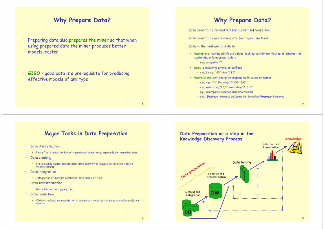
Why Prepare Data?Why Prepare Data?

• Some data preparation is needed for all mining tools

• The purpose of preparation is to transform data sets so that their information content is best exposed to f m pthe mining tool

• Error prediction rate should be lower (or the same) after the preparation as before it

4

Why Prepare Data?Why Prepare Data?

• Preparing data also prepares the miner so that when i d d t th i d b tt using prepared data the miner produces better

models, faster

• GIGO - good data is a prerequisite for producing effective models of any type

5

Why Prepare Data?Why Prepare Data?• Data need to be formatted for a given software tool

• Data need to be made adequate for a given method

D h l ld d• Data in the real world is dirty

• incomplete: lacking attribute values, lacking certain attributes of interest, or containing only aggregate datacontaining only aggregate data

• e.g., occupation=“”

• noisy: containing errors or outliers• e.g., Salary=“-10”, Age=“222”

• inconsistent: containing discrepancies in codes or names• e g Age=“42” Birthday=“03/07/1997”• e.g., Age= 42 Birthday= 03/07/1997

• e.g., Was rating “1,2,3”, now rating “A, B, C”

• e.g., discrepancy between duplicate records

6

• e.g., Endereço: travessa da Igreja de Nevogilde Freguesia: Paranhos

Major Tasks in Data PreparationMajor Tasks in Data Preparation

• Data discretizationData discretization

• Part of data reduction but with particular importance, especially for numerical data

• Data cleaningg

• Fill in missing values, smooth noisy data, identify or remove outliers, and resolve inconsistencies

• Data integration• Data integration

• Integration of multiple databases, data cubes, or files

• Data transformation

• Normalization and aggregation

• Data reduction

• Obtains reduced representation in volume but produces the same or similar analytical results

7

Data Preparation as a step in the Data Preparation as a step in the Knowledge Discovery Process

Evaluation and P t ti

Knowledge

Presentation

Data Mining

Selection and Transformation

Cleaning and Integration DW

8

DB

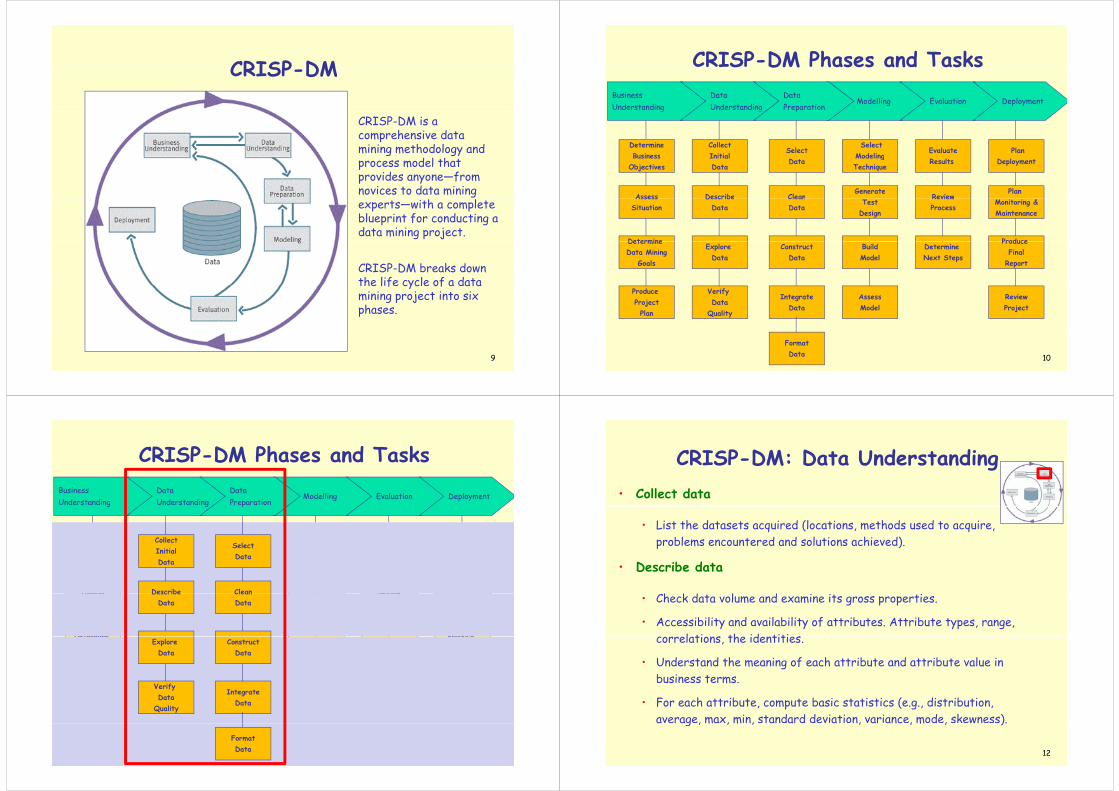
CRISP DMCRISP-DM

CRISP-DM is a comprehensive data mining methodology and g gyprocess model that provides anyone—from novices to data mining experts—with a complete blueprint for conducting a data mining project.

CRISP-DM breaks down the life cycle of a data the life cycle of a data mining project into six phases.

9

CRISP-DM Phases and Tasks

Modelling Evaluation DeploymentBusiness Understanding

DataUnderstanding

DataPreparation

SelectModeling

Evaluate Plan

g

DetermineBusiness

g p

CollectInitial

SelectModelingTechnique

Generate

Results

Review

Deployment

Plan

BusinessObjectives

Assess

InitialData

Describe

Data

CleanTest

Design

ReviewProcess

Monitoring &Maintenance

Produce

AssessSituation

Determine

DescribeData

CleanData

BuildModel

Determine Next Steps

Produce Final

Report

Determine Data Mining

Goals

Explore Data

ConstructData

AssessModel

ReviewProject

Produce ProjectPlan

Verify Data

Quality

IntegrateData

10

FormatData

CRISP-DM Phases and Tasks

Modelling Evaluation DeploymentBusiness Understanding

DataUnderstanding

DataPreparation

SelectModeling

Evaluate Plan

g

DetermineBusiness

g p

CollectInitial

SelectModelingTechnique

Generate

Results

Review

Deployment

Plan

BusinessObjectives

Assess

InitialData

Describe

Data

CleanTest

Design

ReviewProcess

Monitoring &Maintenance

Produce

AssessSituation

Determine

DescribeData

CleanData

BuildModel

Determine Next Steps

Produce Final

Report

Determine Data Mining

Goals

Explore Data

ConstructData

AssessModel

ReviewProject

Produce ProjectPlan

Verify Data

Quality

IntegrateData

11

FormatData

CRISP-DM: Data Understanding• Collect data

CRISP DM: Data Understanding

• List the datasets acquired (locations, methods used to acquire, problems encountered and solutions achieved).

• Describe data

h k l • Check data volume and examine its gross properties.

• Accessibility and availability of attributes. Attribute types, range, c rrel ti ns the identitiescorrelations, the identities.

• Understand the meaning of each attribute and attribute value in business termsbusiness terms.

• For each attribute, compute basic statistics (e.g., distribution, average, max, min, standard deviation, variance, mode, skewness).

12

a rag , ma , m n, tan ar at n, ar anc , m , wn ).

CRISP-DM: Data Understanding•Explore data

• Analyze properties of interesting attributes in detail

g

• Analyze properties of interesting attributes in detail.• Distribution, relations between pairs or small numbers of attributes, properties

of significant sub-populations, simple statistical analyses.

•Verify data quality

• Identify special values and catalogue their meaning.Identify special values and catalogue their meaning.

• Does it cover all the cases required? Does it contain errors and how common are they?

• Identify missing attributes and blank fields. Meaning of missing data.

• Do the meanings of attributes and contained values fit together?

• Check spelling of values (e.g., same value but sometime beginning with a lower case letter, sometimes with an upper case letter).

• Check for plausibility of values e g all fields have the same or nearly the

13

Check for plausibility of values, e.g. all fields have the same or nearly the same values.

CRISP-DM: Data Preparation

• Select data

CRISP DM: Data Preparation

• Reconsider data selection criteria. • Decide which dataset will be used.• Collect appropriate additional data (internal or external).• Consider use of sampling techniques.• Explain why certain data was included or excluded.

• Clean data

• Correct, remove or ignore noise. • Decide how to deal with special values and their meaning (99 for

marital status).• Aggregation level, missing values, etc.• Outliers?

14

• Outliers?

CRISP-DM: Data Preparation• Construct data

D i d tt ib t

CRISP DM: Data Preparation

• Derived attributes.• Background knowledge.• How can missing attributes be constructed or imputed?How can missing attributes be constructed or imputed?

• Integrate data

I d l ( bl d d )• Integrate sources and store result (new tables and records).

• Format Data

• Rearranging attributes (Some tools have requirements on the order of the attributes, e.g. first field being a unique identifier for each record or last field being the outcome field the model is to predict).

• Reordering records (Perhaps the modelling tool requires that the records be sorted according to the value of the outcome attribute).

• Reformatted within-value (These are purely syntactic changes made to satisfy

15

Reformatted within value (These are purely syntactic changes made to satisfy the requirements of the specific modelling tool, remove illegal characters, uppercase lowercase).

TYPES OF DATA AND BASIC

STATISTICS

16

T f D t M tTypes of Data Measurements

• Measurements differ in their nature and the Measurements differ in their nature and the amount of information they give

Q lit ti Q tit ti• Qualitative vs. Quantitative

17

Types of MeasurementsTypes of Measurements

• Nominal scale• Nominal scale

• Categorical scaleQualitative

More in

• Ordinal scaleQualitative nform

atio

• Interval scale

• Ratio scale Quantitative

on contentt

Discrete or Continuous

18

Types of Measurements: ExamplesTypes of Measurements: Examples• Nominal:

• ID numbers, Names of people

• Categorical:Categorical:

• eye color, zip codes

O di l• Ordinal:

• rankings (e.g., taste of potato chips on a scale from 1-10), grades, height in {tall medium short}height in {tall, medium, short}

• Interval:

• calendar dates, temperatures in Celsius or Fahrenheit, GRE score

• Ratio:

19

• temperature in Kelvin, length, time, counts

Types of Measurements: ExamplesDay Outlook Temperature Humidity Wind PlayTennis? 1 Sunny 85 85 Light No

Types of Measurements Examples

2 Sunny 80 90 Strong No 3 Overcast 83 86 Light Yes 4 Rain 70 96 Light Yes 5 R i 68 80 Li h Y 5 Rain 68 80 Light Yes 6 Rain 65 70 Strong No 7 Overcast 64 65 Strong Yes 8 S 72 95 Li ht N

Day Outlook Temperature Humidity Wind PlayTennis? 1 Sunny Hot High Light No 2 Sunny Hot High Strong No

8 Sunny 72 95 Light No 9 Sunny 69 70 Light Yes 10 Rain 75 80 Light Yes 11 Sunny 75 70 Strong Yes

3 Overcast Hot High Light Yes 4 Rain Mild High Light Yes 5 Rain Cool Normal Light Yes 6 R i C l N l S N 11 Sunny 75 70 Strong Yes

12 Overcast 72 90 Strong Yes 13 Overcast 81 75 Light Yes 14 Rain 71 91 Strong No

6 Rain Cool Normal Strong No 7 Overcast Cool Normal Strong Yes 8 Sunny Mild High Light No 9 S C l N l Li ht Y 14 Rain 71 91 Strong No

9 Sunny Cool Normal Light Yes 10 Rain Mild Normal Light Yes 11 Sunny Mild Normal Strong Yes 12 Overcast Mild High Strong Yes

20

12 Overcast Mild High Strong Yes 13 Overcast Hot Normal Light Yes 14 Rain Mild High Strong No

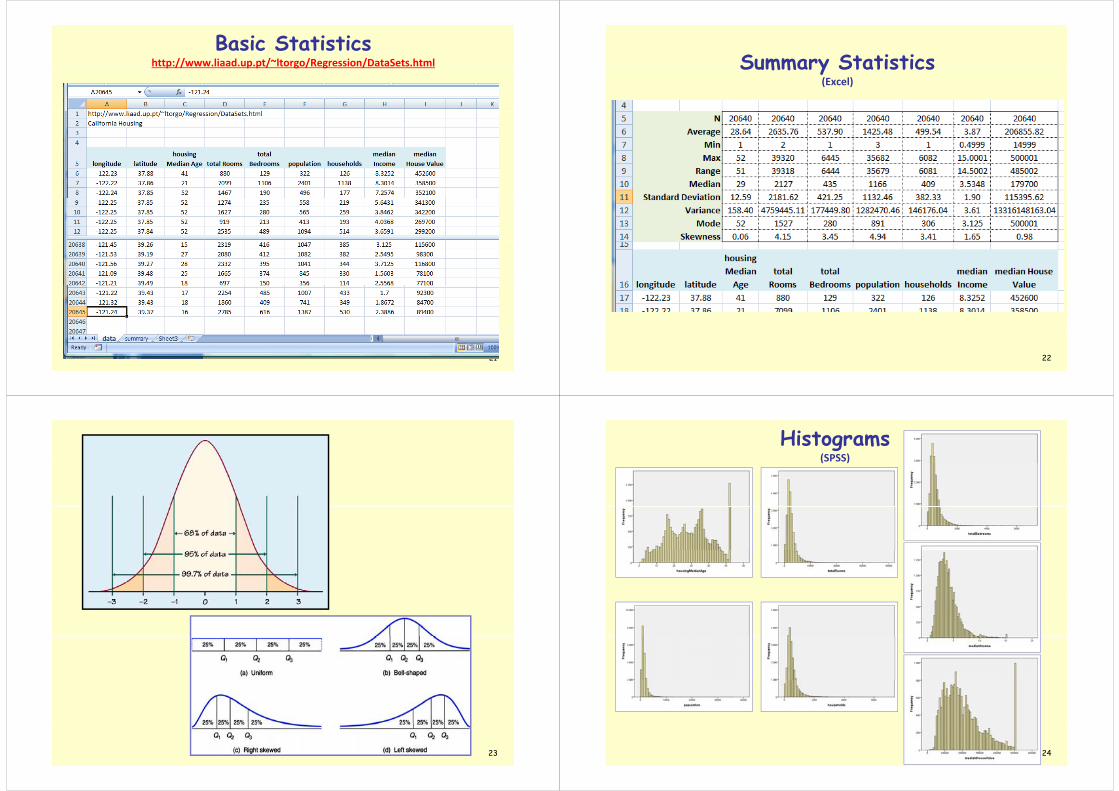
Basic Statisticshttp://www.liaad.up.pt/~ltorgo/Regression/DataSets.htmlp p p g g

21

Summary StatisticsSummary Statistics(Excel)

22

23

Histograms(SPSS)

24

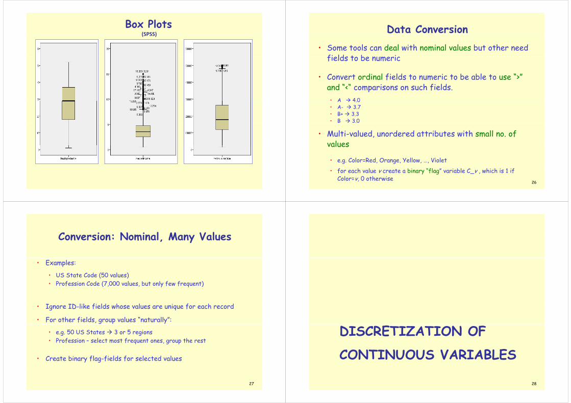
Box Plots(SPSS)(SPSS) Data Conversion

• Some tools can deal with nominal values but other need fields to be numericfields to be numeric

• Convert ordinal fields to numeric to be able to use “>” Convert ordinal fields to numeric to be able to use and “<“ comparisons on such fields.• A 4 0A 4.0• A- 3.7• B+ 3.3• B 3.0

• Multi-valued, unordered attributes with small no. of valuesvalues

• e.g. Color=Red, Orange, Yellow, …, Violet

26

• for each value v create a binary “flag” variable C_v , which is 1 if Color=v, 0 otherwise

Conversion: Nominal Many ValuesConversion: Nominal, Many Values

• Examples:

• US State Code (50 values)• Profession Code (7,000 values, but only few frequent)

• Ignore ID-like fields whose values are unique for each record

• For other fields, group values “naturally”:

• e.g. 50 US States 3 or 5 regions• Profession – select most frequent ones, group the rest

• Create binary flag-fields for selected values

27

DISCRETIZATION OF

CONTINUOUS VARIABLES

28

DiscretizationDiscretization• Divide the range of a continuous attribute into intervalsD th rang of a cont nuous attr ut nto nt r a s

• Some methods require discrete values, e.g. most versions of Naïve Bayes CHAIDNaïve Bayes, CHAID

• Reduce data size by discretization

P f f th l i• Prepare for further analysis

• Discretization is very useful for generating a summary of data

Al ll d “bi i ”• Also called “binning”

29

Equal width BinningEqual-width Binning

• It divides the range into N intervals of equal size (range): uniform gridIt divides the range into N intervals of equal size (range): uniform grid

• If A and B are the lowest and highest values of the attribute, the width of intervals will be: W = (B -A)/N.

T t lTemperature values:64 65 68 69 70 71 72 72 75 75 80 81 83 85

2 2

Count4

2 2 20

Equal Width, bins Low <= value < High

[64,67) [67,70) [70,73) [73,76) [76,79) [79,82) [82,85]

30

q , g

Equal width BinningEqual-width Binning

Count

)

1

[0 – 200,000) … ….

Salary in a corporation

[1,800,000 –2,000,000]

Disadvantage

(a) Unsupervised

(b) Wh d N f

Advantage

(a) simple and easy to implement

31

(b) Where does N come from?

(c) Sensitive to outliers

( ) p y p

(b) produce a reasonable abstraction of data

Equal depth (or height) BinningEqual-depth (or height) Binning

• It divides the range into N intervals, each containing approximately the same number of samples

• Generally preferred because avoids clumping

• In practice, “almost-equal” height binning is used to give more intuitive b kbreakpoints

• Additional considerations:• Additional considerations:

• don’t split frequent values across bins

• create separate bins for special values (e g 0)• create separate bins for special values (e.g. 0)

• readable breakpoints (e.g. round breakpoints

32

Equal depth (or height) BinningEqual-depth (or height) Binning

Temperature values: 64 65 68 69 70 71 72 72 75 75 80 81 83 85

Count

4

Count

4 4

[64 .. .. .. .. 69] [70 .. 72] [73 .. .. .. .. .. .. .. .. 81] [83 .. 85]

2

Equal Height = 4, except for the last bin

[64 .. .. .. .. 69] [70 .. 72] [73 .. .. .. .. .. .. .. .. 81] [83 .. 85]

33

Discretization considerationsDiscretization considerations

• Class-independent methods

• Equal Width is simpler, good for many classesq p , g y• can fail miserably for unequal distributions

• Equal Height gives better results

• Class-dependent methods can be better for classification

• Decision tree methods build discretization on the fly• Decision tree methods build discretization on the fly

• Naïve Bayes requires initial discretization

• Many other methods exist • Many other methods exist …

34

Method 1RMethod 1R

• Developed by Holte (1993).

• It is a supervised discretization method using binning.p g g

• After sorting the data, the range of continuous values is divided into a number of disjoint intervals and the boundaries of those intervals are jadjusted based on the class labels associated with the values of the feature.

• Each interval should contain a given minimum of instances ( 6 by default) with the exception of the last one.

• The adjustment of the boundary continues until the next values belongs to a class different to the majority class in the adjacent interval.

35

1R Example1R ExampleInterval contains at leas 6 elementsAdjustment of the boundary continues until the next values belongs to a class different to the majority class in the adjacent interval.

1 2 3 4 5 6 1 2 3 4 5 6 7 1 2 3 4 5 6 7 1 2 3 4 5 6 7 1 2 3 4Var 65 78 79 79 81 81 82 82 82 82 82 82 83 83 83 83 83 84 84 84 84 84 84 84 84 84 85 85 85 85 85Class 2 1 2 2 2 1 1 2 1 2 2 2 2 1 2 2 2 1 2 2 1 1 2 2 1 1 1 2 2 2 2

majority 2 2 2 1

new class 1 1 1 1 1 1 1 1 1 1 1 1 1 1 1 1 1 1 1 1 2 2 2 2 2 2 2 3 3 3 3class 1 1 1 1 1 1 1 1 1 1 1 1 1 1 1 1 1 1 1 1 2 2 2 2 2 2 2 3 3 3 3

36

ExerciseExercise

• Discretize the following values using EW and ED binning

• 13 15 16 16 19 20 21 22 22 25 30 33 35 35 36 40 4513, 15, 16, 16, 19, 20, 21, 22, 22, 25, 30, 33, 35, 35, 36, 40, 45

37

Entropy Based DiscretizationEntropy Based DiscretizationClass dependent (classification)p

1. Sort examples in increasing order

2 Each value forms an interval (‘m’ intervals)2. Each value forms an interval ( m intervals)

3. Calculate the entropy measure of this discretization

4 Find the binary split boundary that minimizes the entropy function 4. Find the binary split boundary that minimizes the entropy function over all possible boundaries. The split is selected as a binary discretization.

| | | |S S

5 A l th i l til t i it i i t

1 21 2

| | | |( , ) ( ) ( )| | | |

E S T Ent EntS SS SS S

5. Apply the process recursively until some stopping criterion is met, e.g.,

( ) ( , )Ent S E T S δ

38

1 E tEntropy

p 1-p Ent0.2 0.8 0.720.4 0.6 0.970 5 0 5 10.5 0.5 10.6 0.4 0.970.8 0.2 0.72

log2(2)

p1 p2 p3 Ent0.1 0.1 0.8 0.920.2 0.2 0.6 1.370.1 0.45 0.45 1.370 2 0 4 0 4 1 52l ( ) log

NEnt p p

39

0.2 0.4 0.4 1.520.3 0.3 0.4 1.57

0.33 0.33 0.33 1.58

log2(3)21

logc cc

Ent p p

Ent p /Imp itEntropy/Impurity

S i i C C l• S - training set, C1,...,CN classes

• Entropy E(S) - measure of the impurity in a group of examples

• p - proportion of C in Spc proportion of Cc in S

N

21

Impurity( ) logc cc

S p p

40

ImpurityImpurity

Very impure group Less impure Minimum impuritymp Minimum impurity

41

An example of entropy disc.

Test split temp < 71.5 yes no

< 71.5 4 2Temp. Play?

64 Yes 65 No 2log24log46)571(

splitEnt

> 71.5 5 3

68 Yes 69 Yes 70 Yes

(4 yes, 2 no)

939.03log35log586

log66

log614

)5.71(

splitEnt

71 No 72 No 72 Yes

939.08

log88

log814

yes no72 Yes 75 Yes 75 Yes 80 No

(5 yes, 3 no)

y s no

< 77 7 3

> 77 2 280 No 81 Yes 83 Yes 85 No

103log

103

107log

107

1410)77(

splitEnt

42

85 No 915.0

42log

42

42log

42

144

An example (cont.)Temp. Play?

64 Yes 6th splitThe method tests all split possibilities and chooses

65 No 68 Yes 69 Yes

p possibilities and chooses the split with smallest entropy.

69 Yes 70 Yes 71 No 72 No 4 h li

5th splitIn the first iteration a split at 84 is chosen.

72 No 72 Yes 75 Yes 75 Yes 3rd split

4th split The two resulting branches are processed recursively.

75 Yes 80 No 81 Yes 83 Yes

2nd split The fact that recursion l i th fi t 83 Yes

85 No 1st split

only occurs in the first interval in this example is an artifact. In general both intervals have to be

43

both intervals have to be split.

The stopping criterionThe stopping criterion

Previous slide did not take into account the stopping criterion

Ent S E T S( ) ( , )

Previous slide did not take into account the stopping criterion.

NST

NN ),()1log(

NN

)]()()([)23(log)( SEntcSEntcScEntTS c )]()()([)23(log),( 22112 SEntcSEntcScEntTS

c is the number of classes in Sc is the number of classes in Sc1 is the number of classes in S1c2 is the number of classes in S2. 

44

2 2

This is called the Minimum Description Length Principle (MDLP)

ExerciseExercise

• Compute the gain of splitting this data in halfCompute the gain of splitting this data in halfHumidity play

65 Yes70 No70 Yes70 Yes70 Yes75 Yes80 Yes80 Yes80 Yes85 No86 Yes90 No90 Yes91 No

45

95 No96 Yes

WORKING IN THE

ENVIRONMENT

46

Brief Introduction to RBrief Introduction to R

• http://www.r-project.org/• http://cran.r‐project.org/doc/contrib/Short‐refcard.pdf 

• Examples of Expressions:• 3+5*6• 3+5 6

• a <‐ 2+2  (atribuir resultado de expressão a uma variável)

• 3^(3+2)( )

• b <‐ 1:10 (define sequência)

• b*3

• log(b)

• b+2

( ) ( f ê )

47

• seq(1,15,2) (define sequência)

more R examplesmore R examples

• ?log – help on a function• help.search(“clustering”)• objects() – lists existing objectsobjects()  lists existing objects• rm(obj1, obj2,...) – removes existing objects• str(obj)   – displays the internal structure of an object• Menu “File; Change dir ”• Menu  File; Change dir...• dir()

(1 2 3 4 5) d fi t• v <‐ c(1,2,3,4,5)   ‐ defines a vector• m <‐matrix(c(1,2,3,4),2,2) ‐ defines 2x2 matrix de 2x2• a <‐ array(1:8, c(2,2,2))       ‐ defines 2x2x2 array• m*2• m[1,1]• m[1,]

48

The california housing dataset in RThe california housing dataset in R

• File/change dir  ‐ to the directory with the dataset

• cal_housing <‐ read.table("aula_02_dataset_california.txt")

l h [ ] f• cal_housing[1:10,]  ‐ first 10 rows

• cal_housing <‐ read.table("aula_02_dataset_california.txt", header = TRUE) ‐ with headersTRUE)   with headers

• summary(cal_housing) – summary statistics

• hist(cal_housing$totalRooms) – histogram

• hist(cal_housing[,4:4])

• pairs(cal_housing[,3:8]) – scatters for pairs of variables

• plot(cal_housing$population,cal_housing$households) – scatter 2 vars

• cor(cal_housing[,3:8]) – correlation matrix

• boxplot(cal housing[ 3:8]) boxplots

49

• boxplot(cal_housing[,3:8]) ‐ boxplots

Discritization with R Discritization with R • Load Dataset

• data < read table(“aula 02 1R exemplo txt”)• data <‐ read.table( aula_02_1R_exemplo.txt )

• Load Data Preparation Package• library(dprep)

• Equal Width• disc_data_ew <‐ disc.ew(data,1:1)

• disc data ew• disc_data_ew

• Equal Depth• disc_data_ef <‐ disc.ef(data,1:1,3)

• disc_data_ef

• Holte 1R• disc data 1r  <‐ disc.1r(data,1:1,6)_ _ ( , , )

• disc_data_1r

• Entropydi d t t di t (d t 1 2)

50

• disc_data_ent <‐ disc.mentr(data,1:2)

• disc_data_ent

OUTLIERS

51

OutliersOutliers• Outliers are values thought to be out of range.

• “An outlier is an observation that deviates so much from other observations as to arouse suspicion that it was generated by a diff t h i ”different mechanism”

• Can be detected by standardizing observations and label the • Can be detected by standardizing observations and label the standardized values outside a predetermined bound as outliers

• Outlier detection can be used for fraud detection or data cleaning

• Approaches:

• do nothing• enforce upper and lower bounds

l h dl h l52

• let binning handle the problem

Outlier detectionOutlier detection

• Univariate

• Compute mean and std deviation For k=2 or 3 x is an outlier Compute mean and std. deviation. For k=2 or 3, x is an outlier if outside limits (normal distribution assumed)

),( ksxksx

• Boxplot: An observation is an extreme outlier if

(Q1-3IQR, Q3+3IQR), where IQR=Q3-Q1(Q Q , Q Q ), Q Q Q

(IQR = Inter Quartile Range)and declared a mild outlier if it lies outside of the interval

53

m f f(Q1-1.5IQR, Q3+1.5IQR).

54

55

Outlier detectionOutlier detection

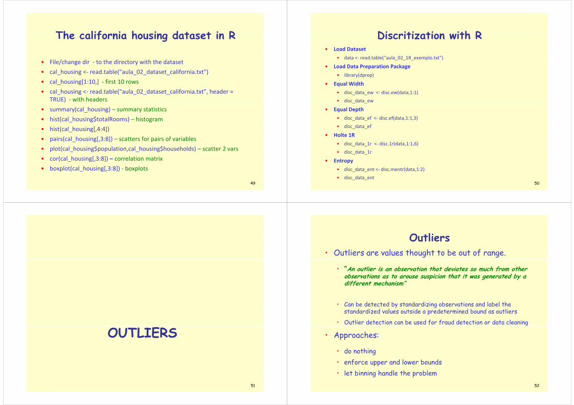
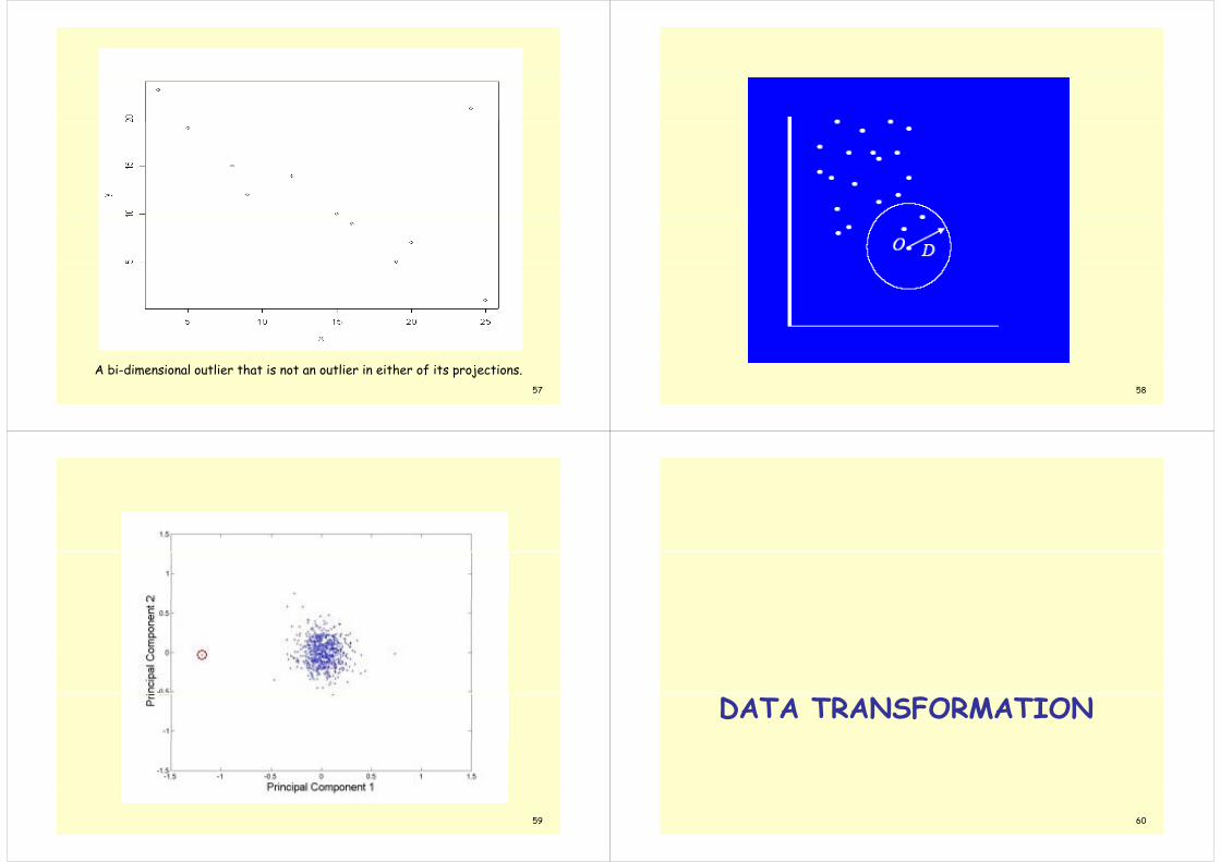
• Multivariate

• Clustering• Very small clusters are outliers

• Distance based• Distance based

• An instance with very few neighbors within λ is regarded tlias an outlier

56

57

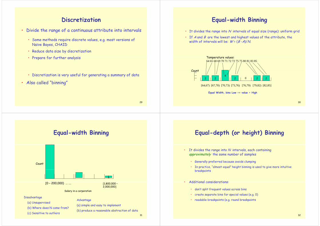
A bi-dimensional outlier that is not an outlier in either of its projections.58

59

DATA TRANSFORMATION

60

Data TransformationData Transformation

• Smoothing: remove noise from data (binning, regression, clustering)

• Aggregation: summarization, data cube construction

Generalization: concept hierarchy climbing• Generalization: concept hierarchy climbing

• Attribute/feature construction

• New attributes constructed from the given ones (add att. area which is based on height and width)

• Normalization

• Scale values to fall within a smaller specified range

61

Scale values to fall within a smaller, specified range

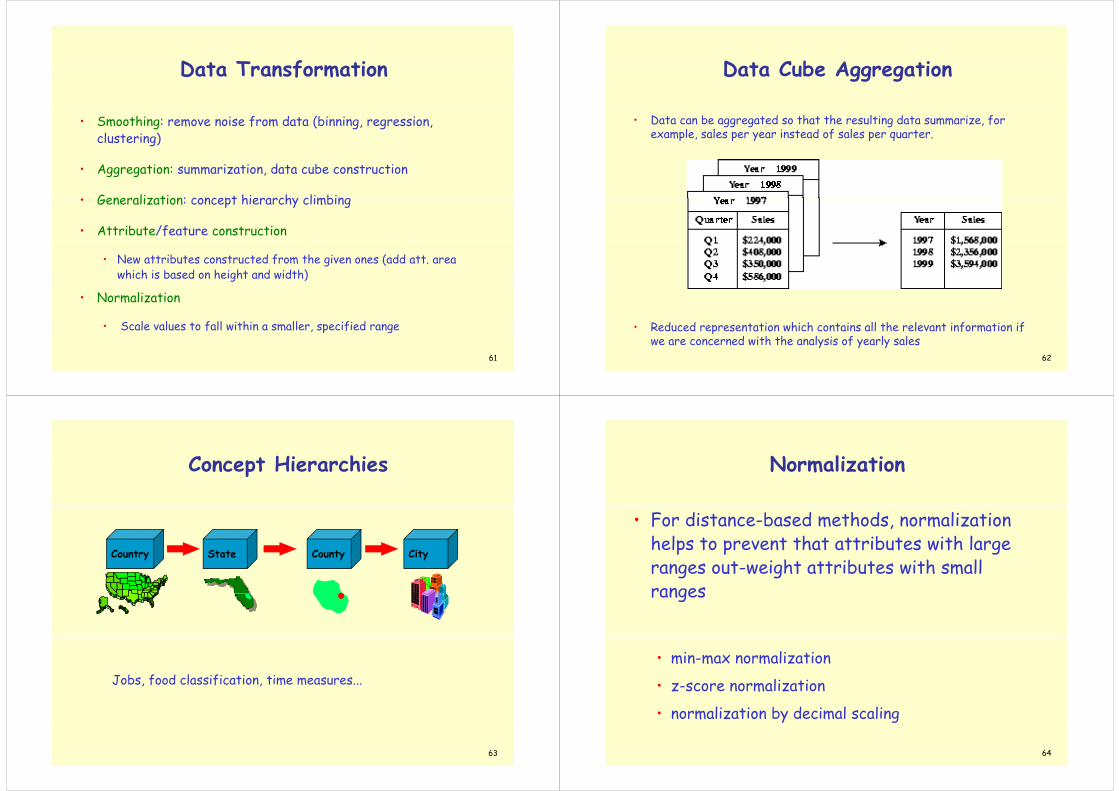
Data Cube AggregationData Cube Aggregation

• Data can be aggregated so that the resulting data summarize, for example, sales per year instead of sales per quarter.

• Reduced representation which contains all the relevant information if

62

Reduced representation which contains all the relevant information if we are concerned with the analysis of yearly sales

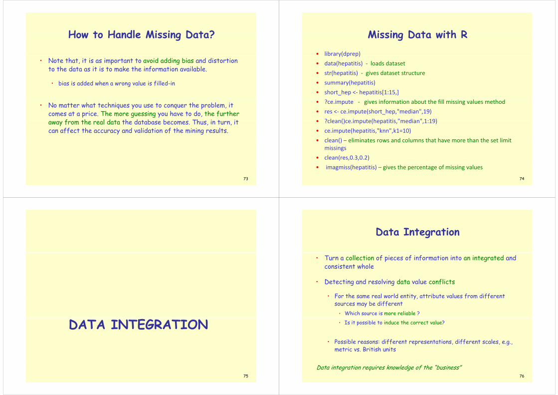
Concept HierarchiesConcept Hierarchies

C S C CiCountry State County City

Jobs food classification time measuresJobs, food classification, time measures...

63

NormalizationNormalization

• For distance-based methods, normalization helps to prevent that attributes with large helps to prevent that attr butes w th large ranges out-weight attributes with small rangesranges

• min-max normalization

li i• z-score normalization

• normalization by decimal scaling

64

NormalizationNormalization

• min-max normalization In Rmin max normalization

min

In R

mmnorm(data,minval=0,maxval=1)

v

min' (new _ max new_min ) new_min

max minv

v v vv v

v

• z-score normalization' v vv

In R

boxplot(znorm(cal housing[ 3:8]))

• normalization by decimal scaling

v boxplot(znorm(cal_housing[,3:8]))

y g

j

vv10

'Where j is the smallest integer such that Max(| |)<1'v

65

range: -986 to 917 => j=3 -986 -> -0.986 917 -> 0.917

MISSING DATA

66

Missing DataMissing Data• Data is not always available

• E.g., many tuples have no recorded value for several attributes, such as customer income in sales data

• Missing data may be due to

• equipment malfunction• inconsistent with other recorded data and thus deleted• data not entered due to misunderstanding• certain data may not be considered important at the time of entrycertain data may not be considered important at the time of entry• not register history or changes of the data

Mi i d t d t b i f d• Missing data may need to be inferred.

• Missing values may carry some information content: e.g. a credit application may carry information by noting which field the applicant did

67

application may carry information by noting which field the applicant did not complete

Missing ValuesMissing Values

• There are always MVs in a real dataset

• MVs may have an impact on modelling in fact they can destroy it!MVs may have an impact on modelling, in fact, they can destroy it!

• Some tools ignore missing values, others use some metric to fill in replacementsreplacements

• The modeller should avoid default automated replacement techniques• Difficult to know limitations, problems and introduced bias

R l i i i l ith t l h t i th t • Replacing missing values without elsewhere capturing that information removes information from the dataset

68

How to Handle Missing Data?How to Handle Missing Data?

• Ignore records (use only cases with all values)

• Usually done when class label is missing as most prediction methods y g pdo not handle missing data well

• Not effective when the percentage of missing values per attribute i id bl it l d t i ffi i t d/ bi d varies considerably as it can lead to insufficient and/or biased

sample sizes

• Ignore attributes with missing valuesIgnore attributes with missing values

• Use only features (attributes) with all values (may leave out important features)important features)

• Fill in the missing value manually

69

• tedious + infeasible?

How to Handle Missing Data?How to Handle Missing Data?

• Use a global constant to fill in the missing value

• e.g., “unknown”. (May create a new class!)g , ( y )

• Use the attribute mean to fill in the missing valueUse the attr bute mean to f ll n the m ss ng value

• It will do the least harm to the mean of existing data

If the mean is to be unbiased• If the mean is to be unbiased

• What if the standard deviation is to be unbiased?

• Use the attribute mean for all samples belonging to the same class to fill in the missing value

70

class to fill in the missing value

How to Handle Missing Data?How to Handle Missing Data?

• Use the most probable value to fill in the missing value

• Inference-based such as Bayesian formula or decision treey

• Identify relationships among variables• Linear regression, Multiple linear regression, Nonlinear regression

• Nearest-Neighbour estimator• Finding the k neighbours nearest to the point and fill in the most

frequent value or the average valueq g

• Finding neighbours in a large dataset may be slow

71

Nearest Neighbour Nearest-Neighbour

72

How to Handle Missing Data?How to Handle Missing Data?

• Note that, it is as important to avoid adding bias and distortion to the data as it is to make the information available.

• bias is added when a wrong value is filled-in

• No matter what techniques you use to conquer the problem, it comes at a price. The more guessing you have to do, the further

f th l d t th d t b b Th i t it away from the real data the database becomes. Thus, in turn, it can affect the accuracy and validation of the mining results.

73

Missing Data with RMissing Data with R• library(dprep)library(dprep)

• data(hepatitis)  ‐ loads dataset

• str(hepatitis)  ‐ gives dataset structure

• summary(hepatitis) 

• short_hep <‐ hepatitis[1:15,]

• ?ce.impute   ‐ gives information about the fill missing values method

• res <‐ ce.impute(short_hep,"median",19)

• ?clean()ce impute(hepatitis "median" 1:19)• ?clean()ce.impute(hepatitis, median ,1:19)

• ce.impute(hepatitis,"knn",k1=10)

• clean() – eliminates rows and columns that have more than the set limitclean()  eliminates rows and columns that have more than the set limit missings

• clean(res,0.3,0.2)

74

• imagmiss(hepatitis) – gives the percentage of missing values 

DATA INTEGRATION

75

Data IntegrationData Integration

• Turn a collection of pieces of information into an integrated and consistent whole

• Detecting and resolving data value conflicts

• For the same real world entity attribute values from different • For the same real world entity, attribute values from different sources may be different

• Which source is more reliable ?

• Is it possible to induce the correct value?

P ibl diff i diff l • Possible reasons: different representations, different scales, e.g., metric vs. British units

76

Data integration requires knowledge of the “business”

Types of Inter-schema Conflictsyp

• Classification conflictsClassification conflicts

• Corresponding types describe different sets of real world elements. DB1: authors of journal and conference papers; DB1 authors of journal and conference papers;

DB2 authors of conference papers only.• Generalization / specialization hierarchy

• Descriptive conflicts

• naming conflicts : synonyms , homonyms

• cardinalities: first name - one , two , N valuescardinalities first name one , two , N values

• domains: salary : $, Euro ... ; student grade : [ 0 : 20 ] , [1 : 5 ]• Solution depends upon the type of the descriptive conflict

77

Data type inconsistency exampleData type inconsistency example

• 1999 Sep 23The $125 million Mars Climate Orbiter was presumed lost after it hit the Martian atmosphere The crash was later blamed on it hit the Martian atmosphere. The crash was later blamed on navigation confusion due to 2 teams using conflicting English and metric units.

• http://en.wikipedia.org/wiki/Mars Climate Orbiterhttp //en.w k ped a.org/w k /Mars_ l mate_Orb ter

78

Types of Inter-schema Conflictsyp

• Structural conflicts

• DB1 : Book is a class; DB2 : books is an attribute of Author• Choose the less constrained structure (Book is a class)

• Fragmentation conflicts

• DB1: Class Road_segment ; DB2: Classes Way_segment , Separator

• Aggregation relationship

79

H dli R d d i D t I t tiHandling Redundancy in Data Integration

• Redundant data occur often when integrating databases

• The same attribute may have different names in different databasesy

• False predictors are fields correlated to target behavior, which describe events that happen at the same time or after the target b h ibehavior

• Example: Service cancellation date is a leaker when predicting attriters

• One attribute may be a “derived” attribute in another table, e.g., annual revenue

• For numerical attributes, redundancymay be detected by correlation analysis

11

11

11

11

1

2

1

2

1

XYN

nn

N

nn

N

nnn

XY ryy

Nxx

N

yyxxNr

80

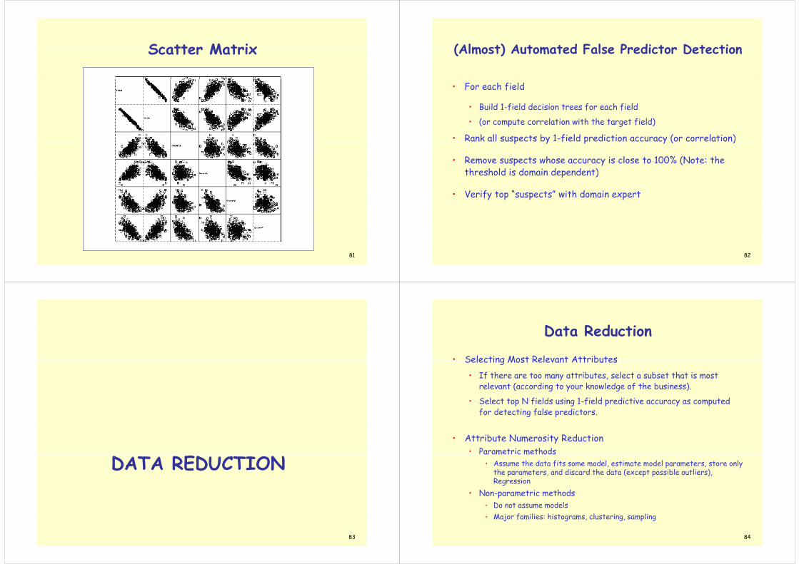
Scatter MatrixScatter Matrix

81

(Almost) Automated False Predictor Detection(Almost) Automated False Predictor Detection

• For each field

• Build 1-field decision trees for each field

• (or compute correlation with the target field)

• Rank all suspects by 1-field prediction accuracy (or correlation)Rank all suspects by f eld pred ct on accuracy (or correlat on)

• Remove suspects whose accuracy is close to 100% (Note: the threshold is domain dependent)threshold is domain dependent)

• Verify top “suspects” with domain expert

82

DATA REDUCTION

83

Data ReductionData Reduction

• Selecting Most Relevant AttributesSelecting Most Relevant Attributes• If there are too many attributes, select a subset that is most

relevant (according to your knowledge of the business).

• Select top N fields using 1-field predictive accuracy as computed for detecting false predictors.

• Attribute Numerosity Reduction• Parametric methodsParametric methods

• Assume the data fits some model, estimate model parameters, store only the parameters, and discard the data (except possible outliers), Regressiong

• Non-parametric methods• Do not assume models

Major families: histograms clustering sampling

84

• Major families: histograms, clustering, sampling

ClusteringClustering

• Partition a data set into clusters makes it possible to store cluster representation only

• Can be very effective if data is clustered but not if data is “smeared”

• There are many choices of clustering definitions and clustering algorithms, further detailed in next lessonsg

85

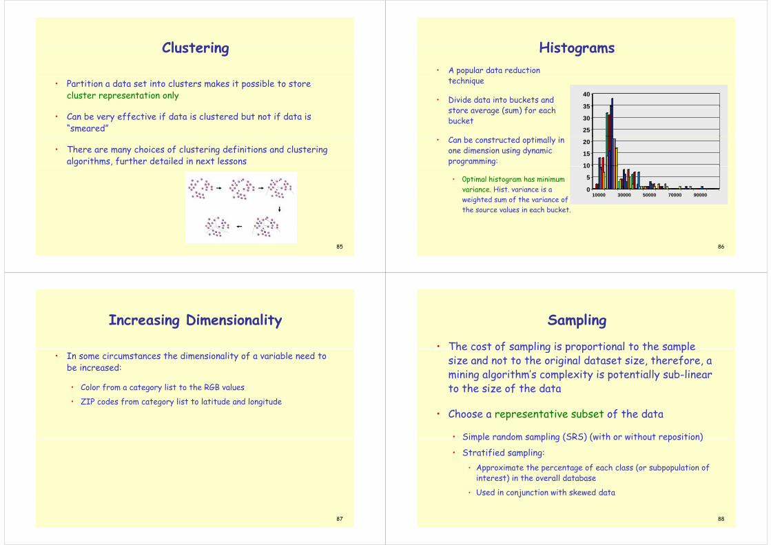
HistogramsHistograms• A popular data reduction

technique

• Divide data into buckets and 35

40

store average (sum) for each bucket

b d ll 25

30

35

• Can be constructed optimally in one dimension using dynamic programming: 10

15

20

• 0ptimal histogram has minimum variance. Hist. variance is a 0

5

10

10000 30000 50000 70000 90000weighted sum of the variance of the source values in each bucket.

10000 30000 50000 70000 90000

86

Increasing DimensionalityIncreasing Dimensionality

• In some circumstances the dimensionality of a variable need to be increased:

• Color from a category list to the RGB values

• ZIP codes from category list to latitude and longitude

87

SamplingSampling

• The cost of sampling is proportional to the sample The cost of sampling is proportional to the sample size and not to the original dataset size, therefore, a mining algorithm’s complexity is potentially sub-linear g g p y p yto the size of the data

• Choose a representative subset of the data

• Simple random sampling (SRS) (with or without reposition)Simple random sampling (SRS) (with or without reposition)

• Stratified sampling: • Approximate the percentage of each class (or subpopulation of Approximate the percentage of each class (or subpopulation of

interest) in the overall database

• Used in conjunction with skewed data

88

Unbalanced Target DistributionUnbalanced Target Distribution

• Sometimes, classes have very unequal frequency

• Attrition prediction: 97% stay, 3% attrite (in a month)p y, ( )

• medical diagnosis: 90% healthy, 10% disease

• eCommerce: 99% don’t buy, 1% buyy y

• Security: >99.99% of Americans are not terrorists

• Similar situation with multiple classesp

• Majority class classifier can be 97% correct, but useless

89

Handling Unbalanced DataHandling Unbalanced Data

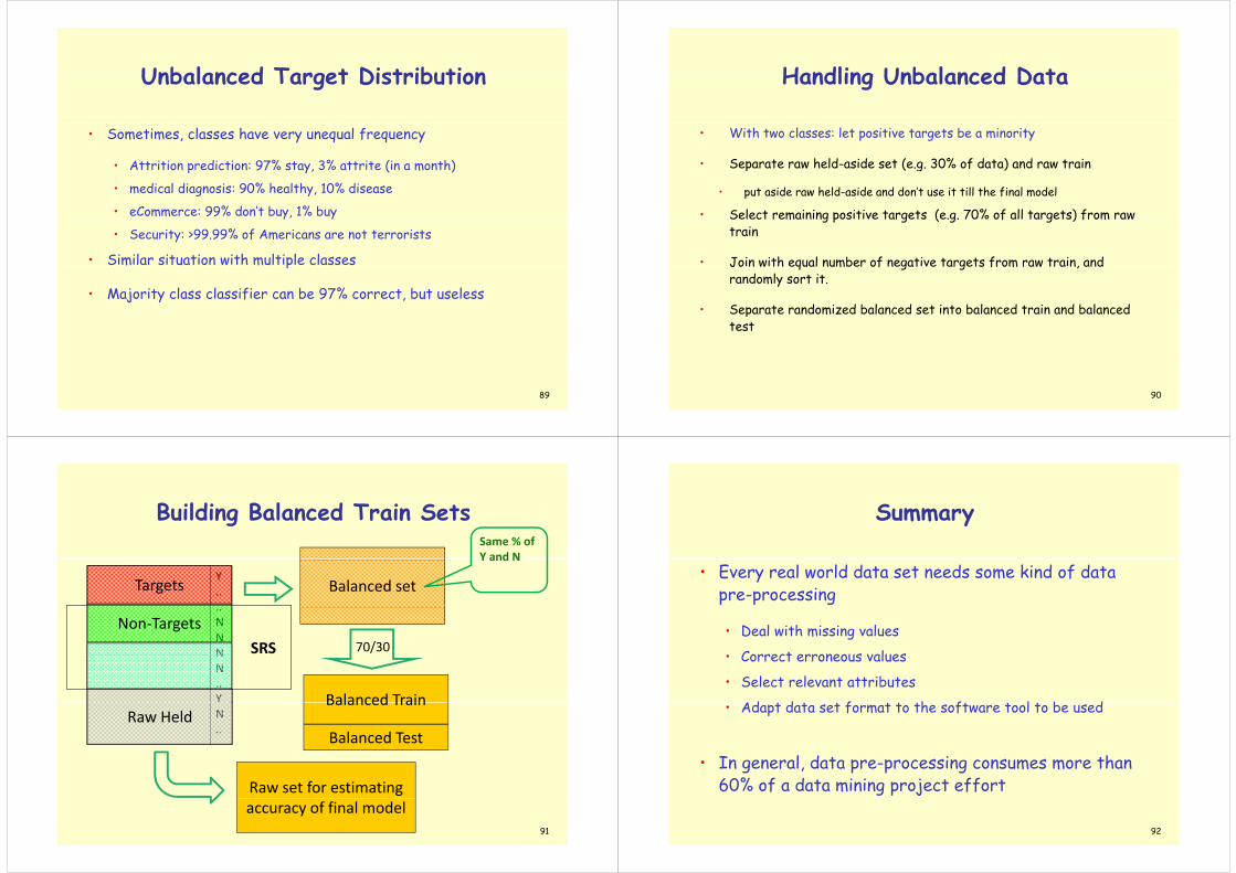
• With two classes: let positive targets be a minority

• Separate raw held-aside set (e.g. 30% of data) and raw trainp g

• put aside raw held-aside and don’t use it till the final model

• Select remaining positive targets (e.g. 70% of all targets) from raw Select remaining positive targets (e.g. 70% of all targets) from raw train

• Join with equal number of negative targets from raw train, and Jo n w th equal number of negat ve targets from raw tra n, and randomly sort it.

• Separate randomized balanced set into balanced train and balanced p mtest

90

Building Balanced Train SetsBuilding Balanced Train SetsSame % of Y and N

Balanced setY..Targets

Y and N

..NNN

Non‐Targets70/30SRSN

N..Y Balanced TrainN..

Raw HeldBalanced Train

Balanced Test

Raw set for estimating 

91

accuracy of final model

SummarySummary

• Every real world data set needs some kind of data pre-processing

• Deal with missing values

• Correct erroneous values• Correct erroneous values

• Select relevant attributes

Ad t d t t f t t th ft t l t b d• Adapt data set format to the software tool to be used

• In general, data pre-processing consumes more than 60% of a data mining project effort

92

ReferencesReferences

• ‘Data preparation for data mining’, Dorian Pyle, 1999

• ‘Data Mining: Concepts and Techniques’, Jiawei Han and Micheline Data M n ng nc pt an chn qu , J aw Han an M ch n Kamber, 2000

• ‘Data Mining: Practical Machine Learning Tools and Techniques Data Mining: Practical Machine Learning Tools and Techniques with Java Implementations’, Ian H. Witten and Eibe Frank, 1999

• ‘Data Mining: Practical Machine Learning Tools and Techniques Data Mining: Practical Machine Learning Tools and Techniques second edition’, Ian H. Witten and Eibe Frank, 2005

• DM: Introduction: Machine Learning and Data Mining Gregory • DM: Introduction: Machine Learning and Data Mining, Gregory Piatetsky-Shapiro and Gary Parker (http://www.kdnuggets.com/data_mining_course/dm1-introduction-ml-data-mining.ppt)

93

• ESMA 6835 Mineria de Datos (http://math.uprm.edu/~edgar/dm8.ppt)Thank you !!!Thank you !!!

94

Thank you !!!Thank you !!!