Introduction to Clustering - Macquarie Universityweb.science.mq.edu.au/~mjohnson/papers/Johnson14-03Clustering-talk.pdf · Applications of clustering in text processing Evaluating

Introduction to Clustering

Mark Johnson

Department of ComputingMacquarie University

1/57

Outline

Supervised versus unsupervised learning

Applications of clustering in text processing

Evaluating clustering algorithms

Background for the k-means algorithm

The k-means clustering algorithm

Document clustering with k-means clustering

Numerical features in machine learning

Summary

2/57

Data for supervised and unsupervised learning

• In both supervised and unsupervised learning, goal is to map novel itemsto labels

I example 1: map names to their genderI example 2: map documents to their topicI example 3: maps words to their parts of speech

• The difference is the kind of training data usedI in supervised learning the training data contains the labels to be learnt

– example 1: input to supervised learner is[(’Adam’,’male’), (’Eve’,’female’), ...]

I in unsupervised learning the training data does not contain the labels tobe learnt

– example 1: input to unsupervised learner is[’Adam’, ’Eve’, ...]

3/57

Why is unsupervised learning important?

• Supervised learning requires labelled training data

• Manually labelling the training examples is often expensive and slow

⇒ often labelled training data sets are very small

• Unsupervised learning uses unlabelled training data, which is oftencheap and plentiful

• There are semi-supervised learning techniques which can take as input alabelled data set and an unlabelled data set

I usually the labelled data set is much smaller than the unlabelled data setI these typically build on unsupervised learning techniques

4/57

The role of labels in unsupervised classification

• Training data for unsupervised classification does not contain labelsI Name-gender example: input is [’Adam’, ’Eve’, ’Ida’, ...]

⇒ No way to learn the names of the labels (e.g., ’male’,’female’)I but in e.g., document clustering, we can identify key words in documents

in each cluster

⇒ Use arbitrary identifiers as labels (e.g., integers)I In name-gender example: output is [0, 1, 1, ...]

⇒ Since the unsupervised labels are arbitrary, all that matters is whethertwo data items have the same label or different labels

5/57

Unsupervised classification as clustering

• In unsupervised learning, the learner associates unlabelled items withlabels from an arbitrary label set

I In name-gender example:input is [’Adam’, ’Eve’, ’Ida’, ’Bill’, ...]

and output is [0, 1, 1, 0, ...]

• Since the labels are arbitrary, all they do is cluster items into groups

• To convert a labelling into a clustering, put all items with the samelabel into the same cluster

I items with label 0 form cluster ’Adam’, ’Bill’, . . .I items with label 1 form cluster ’Eve’, ’Ida’, . . .

⇒ Unsupervised classification is equivalent to clustering

6/57

Truth in advertising about machine learning

• In supervised learning the labels in the training data tell the learnerwhat to look for

• In unsupervised learning the learner tries to group items that looksimiliar⇒ the features and distance function are more important than in supervised

learning

• Unsupervised learning often returns surprising resultsI you might cluster names in the hope of automatically learning genderI but the clusterer might group them by ethnicity instead!

• Supervised learning works faily reliably if you have good dataI usually most modern supervised classification algorithms have similiar

performanceI too many features doesn’t hurt (so long as there are some informative

features)

• Unsupervised learning is much more uncertainI different algorithms can produce very different resultsI choice of features is extremely important

7/57

Outline








Summary

8/57

Clustering news stories by topic

9/57

Document clustering and keyword identification

• Document clustering identifies thematically-similiar documents in adocument collection

I news stories about the same topic in a collection of news storiesI tweets on related topics from a twitter feedI scientific articles on related topics

• We can use key-word identification methods to identify the mostcharacteristic words in each cluster

I treat each cluster as a giant “meta-document”(i.e., append all of the documents in a document cluster together)

I run Tf.Idf or similiar term-weighting program on the meta-documents toweight the words (and/or phrases) in the “meta-documents”

I identify the words and/or phrases with the highest scores in each“meta-document”

I use these high-scoring words and/or phrases as a label for thecorresponding cluster

10/57

Clustering in search

11/57

Scatter-gather search

Education Iraq Arts Sports Oil Germany LegalDomestic

Scatter

12/57


group of stories


Gather

12/57


Occupation Politics Germany Afghanistan Markets Oil PakistanAfrica

group of stories


Scatter

12/57


smaller group of stories


group of stories


Gather

12/57


S. AfricaW. Africa Security Iraq Iran Nigeria SomaliaTrinidad

smaller group of stories


group of stories


Scatter

12/57

Outline








Summary

13/57

Internal and external measures of clustering accuracy

• Internal measures: A clustering procedure should return a clusteringwhere:

I all data items in the same cluster are very similiar (i.e., “close” to eachother)

I if two data items come from different clusters, then the data items aredifferent (i.e., “distant” from each other)

• External measures: Sometimes for evaluation we can obtain labels for(a subset of) the training data

I labels are not available to clustering program (i.e., clustering program isunsupervised)

I it’s usually not reasonable to expect the clustering program to recover thelabels

I but the labels define a clustering of the data items

– data items with the same label are assigned to the same cluster

I so all we can really do is compare the way that clustering program groupsdata items with the way the labels cluster data items

14/57

Confusion matrices

• Confusion matrices depict therelationship between two clusterings.

• Each cell shows the number of items inthe cross product of the clusterings.

• They can sometimes help us understandjust what a clustering has found.

c1 c2 c3 c4

science 0 4 10 4romance 10 0 1 0politics 0 10 5 12news 1 12 5 10

15/57

Purity

• The purity of a clustering is the fractionof data items assigned to the majoritylabel of each cluster.

• If n is the number of data items andC = (C1, . . . ,Cm) andC ′ = (C ′1, . . . ,C

′m′) are two clusterings

(partitions of the data items), then:

purity(C,C ′) =1

n

m∑k=1

maxj=1:m′

|Ck ∩ C ′j |

• In this example, purity = 44/84 u 0.52

c1 c2 c3 c4

science 0 4 10 4romance 10 0 1 0politics 0 10 5 12news 1 12 5 10

16/57

The problem with purity

• Purity is the fraction of data items assigned to the majority label ofeach cluster

• If the clusters only contain a single data item, whatever label it happensto have will be the majority label of that cluster

⇒ In one-item clusters, the data item in that cluster will have the majoritylabel

⇒ To produce a clustering algorithm that has perfect purity just assigneach data item to its own cluster

I the number of clusters is the number of data items

• Purity is a useful measure if the number of clusters is fixed and muchsmaller than the number of data items

17/57

The Rand Index

• Developed by William Rand in 1971 to avoid problems with purity

• Central idea: given two data items x , x ′ ∈ D, a clustering C eitherplaces them into the same cluster or places them into different clusters

• Given two clusterings C and C ′, the Rand Index R is the number ofpairs x , x ′ ∈ D that are classified the same way by C and C ′ divided bythe total number of pairs x , x ′ ∈ D

I if a is the number of pairs x , x ′ ∈ D that are in the same cluster in C andin the same cluster in C ′, and

I if b is the number of pairs x , x ′ ∈ D that are in different clusters in Cand in different clusters in C ′, and

I n′ = n(n − 1)/2 is the number of pairs x , x ′ ∈ D, then:

R =a + b

n′

18/57

Outline








Summary

19/57

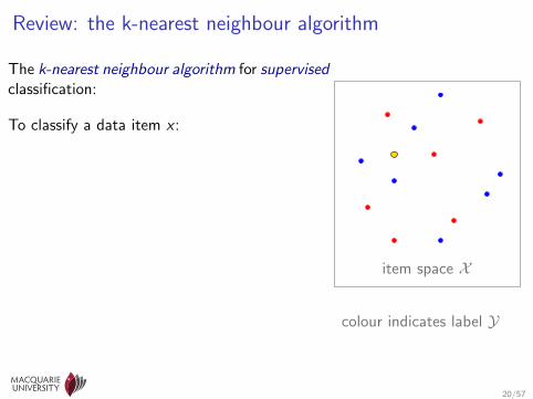
Review: the k-nearest neighbour algorithm

The k-nearest neighbour algorithm for supervisedclassification:

To classify a data item x :

• set N to the k-nearest neighbours of x inD

I the k-nearest neighbours of x are the ktraining items in D with the smallestd(x , x ′) values

• count how often each label y ′ appears in N

• return the most frequent label y in thek-nearest neighbours N of x as thepredicted label for x

item space X

colour indicates label Y

20/57








item space X


20/57








item space X


20/57








item space X


20/57








item space X


20/57

The k-nearest neighbour algorithm

• Let D be a labelled training data set:

D = ((x1, y1), . . . , (xn, yn))

where each item xi ∈ X has label yi ∈ Y• and let d be distance function, where d(x , x ′) is the distance between

two items x , x ′ ∈ X• Given a novel item x ′ to label, the 1-nearest neighbour label y(x ′) is:

y(x) = argminy∈Y

minx∈Dy

d(x , x ′)

where for each y ∈ Y, Dy is the multiset of the training data itemslabelled y , i.e.,

Dy = {x : (x , y) ∈ D}

21/57

The difference between min and argmin• The min of a set of values is the smallest value in a set

I If S = {’Alpha’, ’Beta’, ’Gamma’}I and len(s) returns the length of string sI then

mins∈S

len(s) = 4

• The argmin of a function is the value that minimises that function

argmins∈S

len(s) = ’Beta’

• argmin can also be be used to find the location of the smallest value ina sequence

I If T = (’Alpha’, ’Beta’, ’Gamma’) then:

argmini∈1:3

len(Ti ) = 2

• There are corresponding max and argmax functions as well

22/57

Python code for min and argmin• Python has min and max functions:

>>> xs = (’Alpha’,’Beta’,’Gamma’)

>>> min(xs)

’Alpha’

I with no arguments, min returns the smallest element in a sequence withrespect to Python’s default ordering

• Use comprehensions to compute more complex expressions


>>> min(len(x) for x in xs)

4

computes mins∈S len(s) where S = {’Alpha’, ’Beta’, ’Gamma’}• Use the key argument to specify a function to compute argmin


>>> min(xs, key=len)

’Beta’

computes argmins∈S len(s) where S = {’Alpha’, ’Beta’, ’Gamma’}23/57

More fun with min and max

• To find the location or index of the smallest item in a sequence, useenumerate

>>> xs = (’Gamma’,’Beta’,’Alpha’)

>>> min(enumerate(xs), key=lambda ix: len(ix[1]))[0]

1

computes argmini∈0:n−1 len(Xi )where X = (’Gamma’, ’Beta’, ’Alpha’)

24/57

Understanding argmin with enumerate

• enumerate generates pairs consisting of an index and an object


>>> enumerate(xs)

<enumerate object at 0x7f536dd9d5f0>

>>> list(enumerate(xs))

[(0, ’Alpha’), (1, ’Beta’), (2, ’Gamma’)]

• lambda ix: len(ix[1]) maps a pair to the length of its second element

>>> (lambda ix: len(ix[1]))( (1,’Beta’) )

4

• min(enumerate(xs), key=lambda ix: ix[1]) returns the pair whosesecond element minimises the len function

>>> min(enumerate(xs), key=lambda ix: len(ix[1]))

(1, ’Beta’)

25/57

Informal description of the k-means classification algorithm

• Note: this is not a serious classification algorithm.It is just a stepping stone to the k-means clustering algorithm.

• The k-means classification algorithm:I At training time (i.e., when you have the training data D, but before you

see any test data)

– Given training data D, let Dy be subset of training data items with label y– For each label y , let cy be the mean or centre of Dy

I To classify a new test item x ′:

– for each cluster mean cy , compute dy = distance from cy to x ′

– return the y that minimises dy(i.e., the y such that x ′ is closest to cy )

• This classifier might not be too bad if the Dy are well clustered

26/57

Graphical depiction of k-means classification algorithm

At training time:

• compute cluster means cy

At test time:To classify a new data item x ′:

• compute the distances d(cy , x′) from each

cluster mean cy to x ′

• return the label y of the closest clustermean cy to x ′

item space X


27/57


At training time:






item space X


27/57


At training time:






item space X


27/57


At training time:






item space X


27/57


At training time:






item space X


27/57

The k-means classification algorithm

• Let D be a labelled training data set:

D = ((x1, y1), . . . , (xn, yn))

where each item xi ∈ X has label yi ∈ Y and X is a real-valued vectorspace (i.e., the features have numeric values), and let d be a distancefunction as before

• For each y ∈ Y, let Dy = {x : (x , y) ∈ D}• For each y ∈ Y, let cy be the mean or centre of Dy

cy =1

|Dy |∑x∈Dy

x

• Given a novel item x ′ ∈ X to label, the k-means classification algorithmreturns:

y(x ′) = argminy∈Y

d(cy , x′)

28/57

Review of set size and summation notation

• |S | is number of elements in the set SI If S = {1, 3, 5, 7} then |S | = 4

• If S = {v1, . . . , vn} is a set (or a sequence) of elements vi that can beadded then: ∑

v∈Sv = v1 + . . . + vn

I If S = {1, 3, 5, 7} then∑

v∈S v = 16

I If S = {(1, 2), (5, 4), (2, 2)} then∑

v∈S v = (8, 8)

29/57

Set size and summation in Python

• len returns the size of a set

• sum returns the sum of the values of its arguments

>>> S = set([1,5,10,20])

>>> S

set([1, 10, 20, 5])

>>> len(S)

4

>>> sum(S)

36

30/57

Summing vectors in Python

• Python doesn’t directly support vector arithmeticI but specialised libraries like numpy do

• But it’s easy to sum sequences of vectors

>>> vectors = [(1,5), (2,7), (4,9)]

>>> [sum(vector) for vector in zip(*vectors)]

[7, 21]

>>> zip(*vectors)

[(1, 2, 4), (5, 7, 9)]

31/57

Using Python’s Counter class to count

>>> import collections

>>> cntr = collections.Counter([’a’,’b’,’r’,’a’])

>>> cntr

Counter({’a’: 2, ’r’: 1, ’b’: 1})

>>> cntr[’b’]

1

>>> cntr[’0’] += 1

>>> cntr

Counter({’a’: 2, ’0’: 1, ’r’: 1, ’b’: 1})

>>> cntr.update([’E’,’E’,’N’,’I’,’E’])

>>> cntr

Counter({’E’: 3, ’a’: 2, ’b’: 1, ’I’: 1, ’N’: 1, ’0’: 1, ’r’: 1})

>>> cntr.most_common(2)

[(’E’, 3), (’a’, 2)]

32/57

Outline








Summary

33/57

Informal description of k-means clustering

The k-means clustering algorithm is an iterative algorithm that reassignsdata items to clusters at each iteration

initialise the k cluster centres c1, . . . , ck somehow

repeat until done:

clear the clusters C1, . . . ,Ck

for each training data item x :

find the closest cluster center cj to xadd x to cluster Cj

for each cluster Cj :

set cj to the mean or centre of cluster Cj

34/57

Informal description of k-means clustering

The k-means clustering algorithm is an iterative algorithm that reassignsdata items to clusters at each iteration

initialise the k cluster centres c1, . . . , ck somehow

repeat until done:

clear the clusters C1, . . . ,Ck

for each training data item x :

find the closest cluster center cj to xadd x to cluster Cj

for each cluster Cj :

set cj to the mean or centre of cluster Cj

34/57

Graphical depiction of k-means clustering algorithm

• Unlabelled training data

• Initialise cluster centers somehow

• Move each data item into closest cluster

• Move cluster centres to mean of data items incluster




• No data items moved clusters, so we’re done

item space X

colours show clusters

35/57










item space X


35/57










item space X


35/57










item space X


35/57










item space X


35/57










item space X


35/57










item space X


35/57









• No data items moved clusters, so we’re done item space X


35/57


• Input to k-means clustering algorithm:I Unlabelled training data D = (x1, . . . , xn), where each xi ∈ XI a distance function d , where d(x , x ′) is the distance between x , x ′ ∈ XI the number of clusters k

• K-means clustering algorithm:

Initialise cluster centres cj , for j = 1, . . . , kwhile not converged:

Cj = ∅, for j = 1, . . . , kfor i = 1, . . . , n:j ′ = argminj∈1,...,k d(cj , xi )add xi to Cj′

for j = 1, . . . , k :set cj = mean(Cj)

36/57

Initialising the k-means algorithm

• How the initial cluster centres are chosen makes a big difference to theclusters produced by the k-means algorithm

• There are many different initialisation strategies

• A simple and commonly-used strategy:I pick k different items from the training data at randomI initialise cluster centre cj to the j randomly-chosen item

• Random initialisation ⇒ each run produces different clusters

• Simple initialisation strategies (like this) can result in isolated 1-itemclusters

• Unfortunately even complicated initialisation strategies have draw-backs

37/57

Determining convergence of the k-means algorithm

• Tracing the the number of items moved from one cluster to another,and the intra-cluster distance S

S =∑

i=1,...,k

∑x∈Ci

d(ci , x)

is a good way to monitor convergence.I these usually drops quickly with the first few iterationsI and change very slowly after that

• Often after “enough” iterations no data items are reassigned from onecluster to another

⇒ further iterations will not change cluster assignments⇒ the algorithm has converged

• Unfortunately the k-means algorithm only converges to a localoptimum, which in general is not the global optimum

38/57

Clustering as an optimisation problem

• The intra-cluster distance S (distance from data items to their clustercentres) measures how well the cluster centres describe the data

S =∑

i=1,...,k

∑x∈Ci

d(ci , x)

• The clusters Ci are determined by the cluster centers ci and the dataD = (x1, . . . , xn)

• Goal of clustering: find cluster centres c = (c1, . . . , ck) that minimisethe intra-cluster distance

c = argminc

S

= argminc

∑i=1,...,k

∑x∈Ci

d(ci , x)

• The k-means algorithm is a way of finding cluster centres c thatapproximately minimise the the intra-cluster distance S

39/57

Global and local optima in optimisation problems

• Machine learning algorithms likek-means involve solving anoptimisation problem

I these are usually multi-dimensionalI the graph here only shows 1

dimension

• There can be several local minima

• But only one global minimum

• Iterative optimisation algorithms oftenare attracted into the closest basin ofattraction

z

f (z)

40/57




dimension




z

f (z)

local min.

local min.

40/57




dimension




z

f (z)

global min.

40/57




dimension




z

f (z)

40/57




dimension




z

f (z)

40/57




dimension




z

f (z)

40/57




dimension




z

f (z)

40/57




dimension




z

f (z)

40/57




dimension




z

f (z)

40/57

K-means clustering in Python

class kmeans_clusters:

def __init__(self, data, k, max_iterations, meanf, distf):

self.data = data

self.meanf = meanf

self.distf = distf

self.k = k

self.initial_assignment_of_data_to_clusters()

for iteration in xrange(max_iterations):

self.compute_cluster_centres()

nchanged = self.assign_data_to_closest_clusters()

if nchanged == 0:

break

41/57

Initialising k-means clustering in Python

In class kmeans_clusters:

def initial_assignment_of_data_to_clusters(self):

self.cluster_centres = random.sample(self.data, self.k)

self.cids = [self.closest_cluster(item)

for item in self.data]

def closest_cluster(self, item):

distances = [self.distf(centre, item)

for centre in self.cluster_centres]

closest = min(xrange(self.k), key=lambda j:distances[j])

return closest

• self.cluster_centres is a list of the k cluster centers

• self.cids is a list of the “cluster ids” (integers that index intoself.cluser_centres

• You’ll also need an import random statement at the start of your code

42/57

Computing cluster centres in Python


def compute_cluster_centres(self):

self.cluster_centres =

[self.meanf([item

for item,cid in zip(self.data,self.cids)

if cid == id])

for id in xrange(self.k)]

• This uses the user-supplied function meanf to compute the mean or thecentre of a set of data items

43/57

Updating the clusters in Python


def assign_data_to_closest_clusters(self):

old_cids = self.cids

self.cids = []

nchanged = 0

for i in xrange(len(self.data)):

cid = self.closest_cluster(self.data[i])

self.cids.append(cid)

if cid != old_cids[i]:

nchanged += 1

return nchanged

44/57

Outline








Summary

45/57

Document clustering

• Input: a collection of documentsI we’ll use all 500 documents in nltk.corpus.brownI these are classified into news, popular fiction, etc.I the k-means clusterer won’t see these classesI . . . but we’ll use them to evaluate its output

• We need to provide:I a distance function andI a mean function that computes the centre of a document cluster

• We’ll use a bag of words representation for each documentI each document is represented by a dictionary mapping words to their

frequency countsI for computational efficiency we’ll only use a subset of the vocabulary

46/57

Finding the keywords

import random, re

import nltk, nltk.corpus

word_rex = re.compile(r"^[A-Za-z]+$")

def compute_keywords(corpus, nwords):

cntr = collections.Counter(w.lower()

for w in corpus.words()

if word_rex.match(w))

return set(word for word,count in cntr.most_common(nwords))

• The clusters that the algorithm finds depend on which features it uses

• compute_keywords(corpus, 1000) returns a set containing the the1,000th most frequent words

• We’ll use these words as features

47/57

Mapping fileids to word-frequencies

def fileid_featurevalues(corpus, fileid, keywords):

cntr = collections.Counter(w.lower()

for w in corpus.words(fileid)

if word_rex.match(w) and

w.lower() in keywords)

return cntr

• This returns a dictionary mapping words to their frequencies indocument specified by fileid

• This is a sparse representation of word frequenciesI words with zero frequency are not present in the dictionary

48/57

Distance between two word-frequency dictionaries

def sparse_sum_squared_differences(key_val1, key_val2):

keys = set(key_val1.iterkeys()) | set(key_val2.iterkeys())

return sum(pow(key_val1.get(key,0) - key_val2.get(key,0), 2)

for key in keys)

• key_val1 and key_val2 are two dictionaries mapping words to theirfrequencies

I they represent different documents

• keys is a set containing the union of their keys

• The result is the sum of the square of the differences in the frequencies

49/57

Calculating the cluster means

def sparse_means(key_vals):

keys = set()

keys.update(*(key_val.iterkeys() for key_val in key_vals))

n = len(key_vals)+1e-100

key_meanval = {}

for key in keys:

key_meanval[key] = sum(key_val.get(key,0)

for key_val in key_vals)/n

return key_meanval

• key_vals is a list of word-frequency dictionaries

• keys is a set containing the union of the keys in key_vals

• n is the number of word-frequency dictionaries in key_vals

• key_meanval is a dictionary mapping each key to its mean value

50/57

Outline








Summary

51/57


• The k-means algorithms (and many other machine learning algorithms)require features to have numerical values

• In many applications, features naturally take categorical valuesI in name-gender application, the ’suffix1’ feature takes 1-letter values

and the ’suffix2’ feature takes 2-letter valuesgender features(’Christiana’) = {’suffix1’:’a’,’suffix2’:’na’}

• We’ll re-express these category-valued features as vectors ofBoolean-valued features

I Boolean-valued features are numeric if we treat False = 0 and True = 1

• A feature f can be viewed as a function from items X to feature valuesV (for Boolean features, V = {0, 1})

I suffix1(’Cynthia’) = ’a’

52/57

Re-expressing a categorical feature using Boolean features

• Suppose a categorical feature f ranges over values V = {v1, . . . , vm}I Example: ’suffix1’ ranges over {’a’, . . . , ’z’}

• We re-express a categorical feature pair f with a vectorb = (b1, . . . , bm) of m Boolean-valued features

• If x ∈ X is a data item then:

f (x) = vj ⇔ bj(x) = 1

I Example: If ’suffix1’:’e’ is a feature-value pair for an item then:

b = ( 0, . . . , 0, 1, 0, . . . , 0 )’a’ ’d’ ’e’ ’f’ ’z’

I This is called a one-hot encoding of the feature

• Question: how are the suffix2 features expressed as Boolean features?

53/57

Multiple categorical features as Boolean features

• Each categorical feature can be represented as a vector of Booleanfeatures

• To represent several categorical features, concatenate the vectors ofBoolean features that represent them

• Example:

b = (0, . . . , 0, 1, 0, . . . , 0︸︷︷︸’suffix1’

, 0, . . . , 0, 1, 0, . . . , 0︸︷︷︸’suffix2’

)

54/57

Representations for sparse numerical features

• A set of features is sparse if most features have value 0I when categorical features are converted to binary features, all but one

binary feature has value 0⇒ the resulting binary feature vectors are sparse

• Representing very sparse feature vectors as as standard arrays wastesspace and time

• Idea: only store features whose value is non-zero

• Represent sparse feature vectors as a set of feature:value pairs for eachfeature that has a non-zero value

• if a feature is not represented, its value is zero

• Example: gender features(’Christiana’) = {’suffix1=a’:1,’suffix2=na’:1}

55/57

Outline








Summary

56/57

Summary

• Supervised versus unsupervised learningI unsupervised learning is generally far more challenging

• Unsupervised learning as clustering

• The k-means clustering algorithm

• Confusion matrices as ways of comparing two clusterings

• Evaluating clustering is difficultI cluster purity and its problemsI the Rand index

• The difference between local and global optima, and the problems thiscauses for unsupervised learning

57/57

Documents

Introduction to Clustering - Macquarie Universityweb.science.mq.edu.au/~mjohnson/papers/Johnson14-03Clustering-talk.pdf · Applications of clustering in text processing Evaluating