Introduction to Bayesian Inference

Lecture 2: Key Examples

Tom LoredoDept. of Astronomy, Cornell University

http://www.astro.cornell.edu/staff/loredo/bayes/

CASt Summer School — 8 June 2012

1 / 79

Lecture 2: Key Examples

1 Simple examplesBinary OutcomesNormal DistributionPoisson Distribution

2 Multilevel models for measurement error

3 Bayesian calculation

4 Bayesian Software

5 Closing Reflections

2 / 79

Key Examples

1 Simple examplesBinary OutcomesNormal DistributionPoisson Distribution

2 Multilevel models for measurement error

3 Bayesian calculation

4 Bayesian Software

5 Closing Reflections

3 / 79

Binary Outcomes:

Parameter Estimation

M = Existence of two outcomes, S and F ; for each case or trial,the probability for S is α; for F it is (1− α)

Hi = Statements about α, the probability for success on the nexttrial → seek p(α|D,M)

D = Sequence of results from N observed trials:

FFSSSSFSSSFS (n = 8 successes in N = 12 trials)

Likelihood:

p(D|α,M) = p(failure|α,M) × p(failure|α,M) × · · ·= αn(1− α)N−n

= L(α)

4 / 79

PriorStarting with no information about α beyond its definition,use as an “uninformative” prior p(α|M) = 1. Justifications:

• Intuition: Don’t prefer any α interval to any other of same size• Bayes’s justification: “Ignorance” means that before doing the

N trials, we have no preference for how many will be successes:

P(n success|M) =1

N + 1→ p(α|M) = 1

Consider this a convention—an assumption added to M tomake the problem well posed.

5 / 79

Prior Predictive

p(D|M) =

∫dα αn(1− α)N−n

= B(n+ 1,N − n + 1) =n!(N − n)!

(N + 1)!

A Beta integral, B(a, b) ≡∫dx xa−1(1− x)b−1 = Γ(a)Γ(b)

Γ(a+b) .

6 / 79

Posterior

p(α|D,M) =(N + 1)!

n!(N − n)!αn(1− α)N−n

A Beta distribution. Summaries:

• Best-fit: α = nN= 2/3; 〈α〉 = n+1

N+2 ≈ 0.64

• Uncertainty: σα =√

(n+1)(N−n+1)(N+2)2(N+3)

≈ 0.12

Find credible regions numerically, or with incomplete betafunction

Note that the posterior depends on the data only through n,not the N binary numbers describing the sequence.

n is a (minimal) sufficient statistic.

7 / 79

8 / 79

Binary Outcomes: Model ComparisonEqual Probabilities?

M1: α = 1/2M2: α ∈ [0, 1] with flat prior.

Maximum Likelihoods

M1 : p(D|M1) =1

2N= 2.44× 10−4

M2 : L(α) =

(2

3

)n (1

3

)N−n

= 4.82 × 10−4

p(D|M1)

p(D|α,M2)= 0.51

Maximum likelihoods favor M2 (failures more probable).

9 / 79

Bayes Factor (ratio of model likelihoods)

p(D|M1) =1

2N; and p(D|M2) =

n!(N − n)!

(N + 1)!

→ B12 ≡p(D|M1)

p(D|M2)=

(N + 1)!

n!(N − n)!2N

= 1.57

Bayes factor (odds) favors M1 (equiprobable).

Note that for n = 6, B12 = 2.93; for this small amount ofdata, we can never be very sure results are equiprobable.

If n = 0, B12 ≈ 1/315; if n = 2, B12 ≈ 1/4.8; for extremedata, 12 flips can be enough to lead us to strongly suspectoutcomes have different probabilities.

(Frequentist significance tests can reject null for any sample size.)

10 / 79

Binary Outcomes: Binomial DistributionSuppose D = n (number of heads in N trials), rather than theactual sequence. What is p(α|n,M)?

LikelihoodLet S = a sequence of flips with n heads.

p(n|α,M) =∑

Sp(S |α,M) p(n|S, α,M)

αn (1− α)N−n

J # successes = nK

= αn(1− α)N−nCn,N

Cn,N = # of sequences of length N with n heads.

→ p(n|α,M) =N!

n!(N − n)!αn(1− α)N−n

The binomial distribution for n given α, N.11 / 79

Posterior

p(α|n,M) =

N!n!(N−n)!α

n(1− α)N−n

p(n|M)

p(n|M) =N!

n!(N − n)!

∫dα αn(1− α)N−n

=1

N + 1

→ p(α|n,M) =(N + 1)!

n!(N − n)!αn(1− α)N−n

Same result as when data specified the actual sequence.

12 / 79

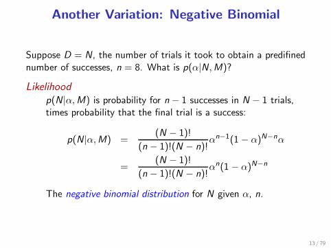
Another Variation: Negative Binomial

Suppose D = N, the number of trials it took to obtain a predifinednumber of successes, n = 8. What is p(α|N,M)?

Likelihoodp(N|α,M) is probability for n− 1 successes in N − 1 trials,times probability that the final trial is a success:

p(N|α,M) =(N − 1)!

(n − 1)!(N − n)!αn−1(1− α)N−nα

=(N − 1)!

(n − 1)!(N − n)!αn(1− α)N−n

The negative binomial distribution for N given α, n.

13 / 79

Posterior

p(α|D,M) = C ′n,N

αn(1− α)N−n

p(D|M)

p(D|M) = C ′n,N

∫dα αn(1− α)N−n

→ p(α|D,M) =(N + 1)!

n!(N − n)!αn(1− α)N−n

Same result as other cases.

14 / 79

Final Variation: “Meteorological Stopping”

Suppose D = (N, n), the number of samples and number ofsuccesses in an observing run whose total number was determinedby the weather at the telescope. What is p(α|D,M ′)?

(M ′ adds info about weather to M.)

Likelihoodp(D|α,M ′) is the binomial distribution times the probabilitythat the weather allowed N samples, W (N):

p(D|α,M ′) = W (N)N!

n!(N − n)!αn(1− α)N−n

Let Cn,N = W (N)(N

n

). We get the same result as before!

15 / 79

Likelihood Principle

To define L(Hi ) = p(Dobs|Hi , I ), we must contemplate what otherdata we might have obtained. But the “real” sample space may bedetermined by many complicated, seemingly irrelevant factors; itmay not be well-specified at all. Should this concern us?

Likelihood principle: The result of inferences depends only on howp(Dobs|Hi , I ) varies w.r.t. hypotheses. We can ignore aspects of theobserving/sampling procedure that do not affect this dependence.

This happens because no sums of probabilities for hypotheticaldata appear in Bayesian results; Bayesian calculations condition onDobs.

This is a sensible property that frequentist methods do not share.Frequentist probabilities are “long run” rates of performance, anddepend on details of the sample space that are irrelevant in aBayesian calculation.

16 / 79

Goodness-of-fit Violates the Likelihood Principle

Theory (H0)The number of “A” stars in a cluster should be 0.1 of thetotal.

Observations5 A stars found out of 96 total stars observed.

Theorist’s analysisCalculate χ2 using nA = 9.6 and nX = 86.4.

Significance level is p(> χ2|H0) = 0.12 (or 0.07 using morerigorous binomial tail area). Theory is accepted.

17 / 79

Observer’s analysisActual observing plan was to keep observing until 5 A starsseen!

“Random” quantity is Ntot, not nA; it should follow thenegative binomial dist’n. Expect Ntot = 50± 21.

p(> χ2|H0) = 0.03. Theory is rejected.

Telescope technician’s analysisA storm was coming in, so the observations would have endedwhether 5 A stars had been seen or not. The proper ensembleshould take into account p(storm) . . .

Bayesian analysisThe Bayes factor is the same for binomial or negative binomiallikelihoods, and slightly favors H0. Include p(storm) if youwant—it will drop out!

18 / 79

Inference With Normals/Gaussians

Gaussian PDF

p(x |µ, σ) = 1

σ√2π

e−(x−µ)2

2σ2 over [−∞,∞]

Common abbreviated notation: x ∼ N(µ, σ2)

Parameters

µ = 〈x〉 ≡∫

dx x p(x |µ, σ)

σ2 = 〈(x − µ)2〉 ≡∫

dx (x − µ)2 p(x |µ, σ)

19 / 79

Gauss’s Observation: Sufficiency

Suppose our data consist of N measurements, di = µ+ ǫi .Suppose the noise contributions are independent, andǫi ∼ N (0, σ2).

p(D|µ, σ,M) =∏

i

p(di |µ, σ,M)

=∏

i

p(ǫi = di − µ|µ, σ,M)

=∏

i

1

σ√2π

exp

[−(di − µ)2

2σ2

]

=1

σN(2π)N/2e−Q(µ)/2σ2

20 / 79

Find dependence of Q on µ by completing the square:

Q =∑

i

(di − µ)2 [Note: Q/σ2 = χ2(µ)]

=∑

i

d2i +

∑

i

µ2 − 2∑

i

diµ

=

(∑

i

d2i

)+ Nµ2 − 2Nµd where d ≡ 1

N

∑

i

di

= N(µ − d)2 +

(∑

i

d2i

)− Nd

2

= N(µ − d)2 + Nr2 where r2 ≡ 1

N

∑

i

(di − d)2

21 / 79

Likelihood depends on {di} only through d and r :

L(µ, σ) = 1

σN(2π)N/2exp

(−Nr2

2σ2

)exp

(−N(µ − d)2

2σ2

)

The sample mean and variance are sufficient statistics.

This is a miraculous compression of information—the normal dist’nis highly abnormal in this respect!

22 / 79

Estimating a Normal Mean

Problem specificationModel: di = µ+ ǫi , ǫi ∼ N(0, σ2), σ is known → I = (σ,M).

Parameter space: µ; seek p(µ|D, σ,M)

Likelihood

p(D|µ, σ,M) =1

σN(2π)N/2exp

(−Nr2

2σ2

)exp

(−N(µ − d)2

2σ2

)

∝ exp

(−N(µ − d)2

2σ2

)

23 / 79

“Uninformative” priorTranslation invariance ⇒ p(µ) ∝ C , a constant.This prior is improper unless bounded.

Prior predictive/normalization

p(D|σ,M) =

∫dµ C exp

(−N(µ − d)2

2σ2

)

= C (σ/√N)

√2π

. . . minus a tiny bit from tails, using a proper prior.

24 / 79

Posterior

p(µ|D, σ,M) =1

(σ/√N)

√2π

exp

(−N(µ − d)2

2σ2

)

Posterior is N(d ,w2), with standard deviation w = σ/√N .

68.3% HPD credible region for µ is d ± σ/√N.

Note that C drops out → limit of infinite prior range is wellbehaved.

25 / 79

Informative Conjugate PriorUse a normal prior, µ ∼ N(µ0,w

20 ).

Conjugate because the posterior is also normal.

PosteriorNormal N(µ, w2), but mean, std. deviation “shrink” towardsprior.

Define B = w2

w2+w20, so B < 1 and B = 0 when w0 is large.

Then

µ = d + B · (µ0 − d)

w = w ·√1− B

“Principle of stable estimation” — The prior affects estimatesonly when data are not informative relative to prior.

26 / 79

Conjugate normal examples:

• Data have d = 3, σ/√N = 1

• Priors at µ0 = 10, with w = {5, 2}

0 5 10 15 20x

0.00

0.05

0.10

0.15

0.20

0.25

0.30

0.35

0.40

0.45

p(x|�

)

Prior

LPost.

0 5 10 15 20x

0.00

0.05

0.10

0.15

0.20

0.25

0.30

0.35

0.40

0.45

p(x| �

)

27 / 79

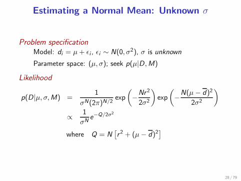
Estimating a Normal Mean: Unknown σ

Problem specificationModel: di = µ+ ǫi , ǫi ∼ N(0, σ2), σ is unknown

Parameter space: (µ, σ); seek p(µ|D,M)

Likelihood

p(D|µ, σ,M) =1

σN(2π)N/2exp

(−Nr2

2σ2

)exp

(−N(µ − d)2

2σ2

)

∝ 1

σNe−Q/2σ2

where Q = N[r2 + (µ− d)2

]

28 / 79

Uninformative PriorsAssume priors for µ and σ are independent.

Translation invariance ⇒ p(µ) ∝ C , a constant.

Scale invariance ⇒ p(σ) ∝ 1/σ (flat in log σ).

Joint Posterior for µ, σ

p(µ, σ|D,M) ∝ 1

σN+1e−Q(µ)/2σ2

29 / 79

Marginal Posterior

p(µ|D,M) ∝∫

dσ1

σN+1e−Q/2σ2

Let τ = Q

2σ2 so σ =√

Q2τ and |dσ| = τ−3/2

√Q2 dτ

⇒ p(µ|D,M) ∝ 2N/2Q−N/2

∫dτ τ

N

2−1e−τ

∝ Q−N/2

30 / 79

Write Q = Nr2[1 +

(µ−d

r

)2]and normalize:

p(µ|D,M) =

(N2 − 1

)!(

N2 − 3

2

)!√π

1

r

[1 +

1

N

(µ− d

r/√N

)2]−N/2

“Student’s t distribution,” with t = (µ−d)

r/√N

A “bell curve,” but with power-law tails

Large N:

p(µ|D,M) ∼ e−N(µ−d)2/2r2

This is the rigorous way to “adjust σ so χ2/dof = 1.”

It doesn’t just plug in a best σ; it slightly broadens posteriorto account for σ uncertainty.

31 / 79

Student t examples:

• p(x) ∝ 1(

1+ x2

n

)n+12

• Location = 0, scale = 1

• Degrees of freedom = {1, 2, 3, 5, 10,∞}

�4 �2 0 2 4x

0.0

0.1

0.2

0.3

0.4

0.5

p(x

)

1

2

3

5

10

normal

32 / 79

Gaussian Background Subtraction

Measure background rate b = b ± σb with source off.

Measure total rate r = r ± σr with source on.

Infer signal source strength s, where r = s + b.

With flat priors,

p(s, b|D,M) ∝ exp

[−(b − b)2

2σ2b

]× exp

[−(s + b − r)2

2σ2r

]

33 / 79

Marginalize b to summarize the results for s (complete the squareto isolate b dependence; then do a simple Gaussian integral overb):

p(s|D,M) ∝ exp

[−(s − s)2

2σ2s

]s = r − bσ2s = σ2r + σ2

b

⇒ Background subtraction is a special case of backgroundmarginalization; i.e., marginalization “told us” to subtract abackground estimate.

Recall the standard derivation of background uncertainty via“propagation of errors” based on Taylor expansion (statistician’sDelta-method).

Marginalization provides a generalization of errorpropagation—without approximation!

34 / 79

Bayesian Curve Fitting & Least SquaresSetup

Data D = {di} are measurements of an underlying functionf (x ; θ) at N sample points {xi}. Let fi(θ) ≡ f (xi ; θ):

di = fi(θ) + ǫi , ǫi ∼ N(0, σ2i )

We seek learn θ, or to compare different functional forms(model choice, M).

Likelihood

p(D|θ,M) =N∏

i=1

1

σi√2π

exp

[−1

2

(di − fi(θ)

σi

)2]

∝ exp

[−1

2

∑

i

(di − fi(θ)

σi

)2]

= exp

[−χ

2(θ)

2

]

35 / 79

Bayesian Curve Fitting & Least Squares

PosteriorFor prior density π(θ),

p(θ|D,M) ∝ π(θ) exp

[−χ

2(θ)

2

]

If you have a least-squares or χ2 code:

• Think of χ2(θ) as −2 logL(θ).

• Bayesian inference amounts to exploration and numericalintegration of π(θ)e−χ2(θ)/2.

36 / 79

Important Case: Separable Nonlinear ModelsA (linearly) separable model has parameters θ = (A, ψ):

• Linear amplitudes A = {Aα}

• Nonlinear parameters ψ

f (x ; θ) is a linear superposition of M nonlinear componentsgα(x ;ψ):

di =M∑

α=1

Aαgα(xi ;ψ) + ǫi

or ~d =∑

α

Aα~gα(ψ) + ~ǫ.

Why this is important: You can marginalize over A analytically→ Bretthorst algorithm (“Bayesian Spectrum Analysis & Param. Est’n” 1988)

Algorithm is closely related to linear leastsquares/diagonalization/SVD.

37 / 79

Poisson Dist’n: Infer a Rate from Counts

Problem:Observe n counts in T ; infer rate, r

Likelihood

L(r) ≡ p(n|r ,M) = p(n|r ,M) =(rT )n

n!e−rT

PriorTwo simple standard choices (or conjugate gamma dist’n):

• r known to be nonzero; it is a scale parameter:

p(r |M) =1

ln(ru/rl)

1

r

• r may vanish; require p(n|M) ∼ Const:

p(r |M) =1

ru

38 / 79

Prior predictive

p(n|M) =1

ru

1

n!

∫ ru

0dr(rT )ne−rT

=1

ruT

1

n!

∫ ruT

0d(rT )(rT )ne−rT

≈ 1

ruTfor ru ≫ n

T

PosteriorA gamma distribution:

p(r |n,M) =T (rT )n

n!e−rT

39 / 79

Gamma Distributions

A 2-parameter family of distributions over nonnegative x , withshape parameter α and scale parameter s:

pΓ(x |α, s) =1

sΓ(α)

(xs

)α−1e−x/s

Moments:

E(x) = sα Var(x) = s2α

Our posterior corresponds to α = n+ 1, s = 1/T .

• Mode r = nT; mean 〈r〉 = n+1

T(shift down 1 with 1/r prior)

• Std. dev’n σr =√

n+1T

; credible regions found by integrating (canuse incomplete gamma function)

40 / 79

41 / 79

The flat priorBayes’s justification: Not that ignorance of r → p(r |I ) = C

Require (discrete) predictive distribution to be flat:

p(n|I ) =

∫dr p(r |I )p(n|r , I ) = C

→ p(r |I ) = C

Useful conventions

• Use a flat prior for a rate that may be zero

• Use a log-flat prior (∝ 1/r) for a nonzero scale parameter

• Use proper (normalized, bounded) priors

• Plot posterior with abscissa that makes prior flat

42 / 79

The On/Off Problem

Basic problem

• Look off-source; unknown background rate bCount Noff photons in interval Toff

• Look on-source; rate is r = s + b with unknown signal sCount Non photons in interval Ton

• Infer s

Conventional solution

b = Noff/Toff ; σb =√Noff/Toff

r = Non/Ton; σr =√Non/Ton

s = r − b; σs =√σ2r + σ2

b

But s can be negative!

43 / 79

Examples

Spectra of X-Ray Sources

Bassani et al. 1989 Di Salvo et al. 2001

44 / 79

Spectrum of Ultrahigh-Energy Cosmic Rays

Nagano & Watson 2000

HiRes Team 2007

log10(E) (eV)F

lux*

E3 /1

024 (

eV2 m

-2 s

-1 s

r-1)

AGASAHiRes-1 MonocularHiRes-2 Monocular

1

10

17 17.5 18 18.5 19 19.5 20 20.5 21

45 / 79

N is Never Large

Sample sizes are never large. If N is too small to get asufficiently-precise estimate, you need to get more data (or makemore assumptions). But once N is ‘large enough,’ you can startsubdividing the data to learn more (for example, in a publicopinion poll, once you have a good estimate for the entire country,you can estimate among men and women, northerners andsoutherners, different age groups, etc etc). N is never enoughbecause if it were ‘enough’ you’d already be on to the nextproblem for which you need more data.

— Andrew Gelman (blog entry, 31 July 2005)

46 / 79

N is Never Large

Sample sizes are never large. If N is too small to get asufficiently-precise estimate, you need to get more data (or makemore assumptions). But once N is ‘large enough,’ you can startsubdividing the data to learn more (for example, in a publicopinion poll, once you have a good estimate for the entire country,you can estimate among men and women, northerners andsoutherners, different age groups, etc etc). N is never enoughbecause if it were ‘enough’ you’d already be on to the nextproblem for which you need more data.

Similarly, you never have quite enough money. But that’s anotherstory.

— Andrew Gelman (blog entry, 31 July 2005)

46 / 79

Bayesian Solution to On/Off Problem

First consider off-source data; use it to estimate b:

p(b|Noff , Ioff ) =Toff(bToff)

Noff e−bToff

Noff !

Use this as a prior for b to analyze on-source data. For on-sourceanalysis Iall = (Ion,Noff , Ioff):

p(s, b|Non) ∝ p(s)p(b)[(s + b)Ton]None−(s+b)Ton || Iall

p(s|Iall) is flat, but p(b|Iall) = p(b|Noff , Ioff), so

p(s, b|Non, Iall) ∝ (s + b)NonbNoff e−sTone−b(Ton+Toff )

47 / 79

Now marginalize over b;

p(s|Non, Iall) =

∫db p(s, b | Non, Iall)

∝∫

db (s + b)NonbNoff e−sTone−b(Ton+Toff )

Expand (s + b)Non and do the resulting Γ integrals:

p(s|Non, Iall) =

Non∑

i=0

Ci

Ton(sTon)ie−sTon

i !

Ci ∝(1 +

Toff

Ton

)i(Non + Noff − i)!

(Non − i)!

Posterior is a weighted sum of Gamma distributions, each assigning adifferent number of on-source counts to the source. (Evaluate viarecursive algorithm or confluent hypergeometric function.)

48 / 79

Example On/Off Posteriors—Short Integrations

Ton = 1

49 / 79

Example On/Off Posteriors—Long Background Integrations

Ton = 1

50 / 79

Second Solution to On/Off Problem

Consider all the data at once; the likelihood is a product of Poissondistributions for the on- and off-source counts:

L(s, b) ≡ p(Non,Noff |s, b, I )∝ [(s + b)Ton]

None−(s+b)Ton × (bToff)Noff e−bToff

Take joint prior to be flat; find the joint posterior and marginalizeover b;

p(s|Non, Ion) =

∫db p(s, b|I )L(s, b)

∝∫

db (s + b)NonbNoff e−sTone−b(Ton+Toff )

→ same result as before.

51 / 79

Third Solution: data augmentationSuppose we knew the number of on-source counts that are fromthe background, Nb. Then the on-source likelihood is simple:

p(Non|s,Nb , Iall) = Pois(Non − Nb; sTon) =(sTon)

Non−Nb

(Non − Nb)!e−sTon

Data augmentation: Pretend you have the “missing data,” thenmarginalize to account for its uncertainty:

p(Non|s, Iall) =

Non∑

Nb=0

p(Nb|Iall) p(Non|s,Nb, Iall)

=∑

Nb

Predictive for Nb × Pois(Non − Nb; sTon)

p(Nb|Iall) =

∫db p(b|Noff , Ioff ) p(Nb|b, Ion)

=

∫db Gamma(b)× Pois(Nb; bTon)

→ same result as before.52 / 79

A profound consistency

We solved the on/off problem in multiple ways, always finding thesame final results.

This reflects something fundamental about Bayesian inference.

R. T. Cox proposed two necessary conditions for a quantification ofuncertainty:

• It should duplicate deductive logic when there is nouncertainty

• Different decompositions of arguments should produce thesame final quantifications (internal consistency)

Great surprise: These conditions are sufficient; they lead to theprobability axioms. E. T. Jaynes and others refined and simplifiedCox’s analysis.

53 / 79

Recap of Key Findings From Examples

• Sufficiency: Model-dependent summary of data

• Conjugate priors

• Likelihood principle

• Marginalization: Generalizes background subtraction,propagation of errors

• Student’s t for handling σ uncertainty

• Exact treatment of Poisson background uncertainty (don’tsubtract!)

54 / 79

Key Examples

1 Simple examplesBinary OutcomesNormal DistributionPoisson Distribution

2 Multilevel models for measurement error

3 Bayesian calculation

4 Bayesian Software

5 Closing Reflections

55 / 79

Complications With Survey Data

• Selection effects (truncation, censoring) — obvious (usually)Typically treated by “correcting” dataMost sophisticated: product-limit estimators

• “Scatter” effects (measurement error, etc.) — insidiousTypically ignored (average out???)

56 / 79

Many Guises of Measurement ErrorAuger data above GZK cutoff (PAO 2007; Soiaporn+ 2011)

QSO hardness vs. luminosity (Kelly 2007, 2011)

57 / 79

Accounting For Measurement Error

Introduce latent/hidden/incidental parameters

Suppose f (x |θ) is a distribution for an observable, x .

From N precisely measured samples, {xi}, we can infer θ from

L(θ) ≡ p({xi}|θ) =∏

i

f (xi |θ)

58 / 79

Graphical representation

• Nodes/vertices = uncertain quantities

• Edges specify conditional dependence

• Absence of an edge denotes conditional independence

θ

x1 x2 xN

L(θ) ≡ p({xi}|θ) =∏

i

f (xi |θ)

59 / 79

But what if the x data are noisy, Di = {xi + ǫi}?

We should somehow incorporate ℓi(xi ) = p(Di |xi )

L(θ, {xi}) ≡ p({Di}|θ, {xi})=

∏

i

ℓi(xi )f (xi |θ)

Marginalize over {xi} to summarize inferences for θ.Marginalize over θ to summarize inferences for {xi}.

Key point: Maximizing over xi and integrating over xi can givevery different results!

60 / 79

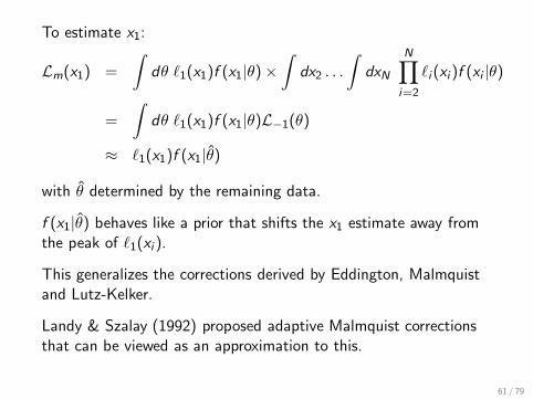
To estimate x1:

Lm(x1) =

∫dθ ℓ1(x1)f (x1|θ)×

∫dx2 . . .

∫dxN

N∏

i=2

ℓi (xi )f (xi |θ)

=

∫dθ ℓ1(x1)f (x1|θ)L−1(θ)

≈ ℓ1(x1)f (x1|θ)

with θ determined by the remaining data.

f (x1|θ) behaves like a prior that shifts the x1 estimate away fromthe peak of ℓ1(xi ).

This generalizes the corrections derived by Eddington, Malmquistand Lutz-Kelker.

Landy & Szalay (1992) proposed adaptive Malmquist correctionsthat can be viewed as an approximation to this.

61 / 79

Graphical representation

DND1 D2

θ

x1 x2 xN

L(θ, {xi}) ≡ p({Di}|θ, {xi})=

∏

i

p(Di |xi )f (xi |θ) =∏

i

ℓi(xi )f (xi |θ)

A two-level multi-level model (MLM).

62 / 79

Bayesian MLMs in Astronomy

Surveys (number counts/“logN–log S”/Malmquist):

• GRB peak flux dist’n (Loredo & Wasserman 1998)

• TNO/KBO magnitude distribution (Gladman+ 1998;Petit+ 2008)

• MLM tutorial; Malmquist-type biases in cosmology(Loredo & Hendry 2009 in BMIC book)

• “Extreme deconvolution” for proper motion surveys(Bovy, Hogg, & Roweis 2011)

Directional & spatio-temporal coincidences:

• GRB repetition (Luo+ 1996; Graziani+ 1996)

• GRB host ID (Band 1998; Graziani+ 1999)

• VO cross-matching (Budavari & Szalay 2008)

63 / 79

Time series:

• SN 1987A neutrinos, uncertain energy vs. time (Loredo& Lamb 2002)

• Multivariate “Bayesian Blocks” (Dobigeon, Tourneret &Scargle 2007)

• SN Ia multicolor light curve modeling (Mandel+ 2009,2011)

Linear regression with measurement error:

• QSO hardness vs. luminosity (Kelly 2007, 2011)

See 2010 CASt Surveys School notes for more!http://astrostatistics.psu.edu/su10/surveys.html

64 / 79

Key Examples

1 Simple examplesBinary OutcomesNormal DistributionPoisson Distribution

2 Multilevel models for measurement error

3 Bayesian calculation

4 Bayesian Software

5 Closing Reflections

65 / 79

Statistical IntegralsInference with independent data

Consider N data, D = {xi}; and model M with m parameters.

Suppose L(θ) = p(x1|θ) p(x2|θ) · · · p(xN |θ).

Frequentist integralsFind long-run properties of procedures via sample spaceintegrals:

I(θ) =∫

dx1 p(x1|θ)∫

dx2 p(x2|θ) · · ·∫

dxN p(xN |θ)f (D, θ)

Rigorous analysis must explore the θ dependence; rarely donein practice.

“Plug-in” approximation: Report properties of procedure forθ = θ. Asymptotically accurate (for large N, expect θ → θ).

“Plug-in” results are easy via Monte Carlo (due toindependence).

66 / 79

Bayesian integrals∫dmθ g(θ) p(θ|M)L(θ) =

∫dmθ g(θ) q(θ)

p(θ|M)L(θ)

• g(θ) = 1 → p(D|M) (norm. const., model likelihood)

• g(θ) = ‘box’ → credible region

• g(θ) = θ → posterior mean for θ

Such integrals are sometimes easy if analytic (especially in lowdimensions), often easier than frequentist counterparts (e.g.,normal credible regions, Student’s t).

Asymptotic approximations: Require ingredients familiarfrom frequentist calculations. Bayesian calculation is notsignificantly harder than frequentist calculation in this limit.

Numerical calculation: For “large” m (> 4 is often enough!)the integrals are often very challenging because of structure(e.g., correlations) in parameter space. This is usually pursuedwithout making any procedural approximations.

67 / 79

Bayesian ComputationLarge sample size: Laplace approximation

• Approximate posterior as multivariate normal → det(covar) factors• Uses ingredients available in χ2/ML fitting software (MLE, Hessian)• Often accurate to O(1/N)

Modest-dimensional models (d<∼10 to 20)

• Adaptive cubature• Monte Carlo integration (importance & stratified sampling, adaptive

importance sampling, quasirandom MC)

High-dimensional models (d>∼5)

• Posterior sampling — create RNG that samples posterior• MCMC is most general framework — Murali’s lab

68 / 79

See SCMA 5 Bayesian Computation tutorial notes for more!

69 / 79

Key Examples

1 Simple examplesBinary OutcomesNormal DistributionPoisson Distribution

2 Multilevel models for measurement error

3 Bayesian calculation

4 Bayesian Software

5 Closing Reflections

70 / 79

Tools for Computational Bayes

Astronomer/Physicist Tools

• BIE http://www.astro.umass.edu/~weinberg/BIE/

Bayesian Inference Engine: General framework for Bayesian inference, tailored toastronomical and earth-science survey data. Built-in database capability tosupport analysis of terabyte-scale data sets. Inference is by Bayes via MCMC.

• CIAO/Sherpa http://cxc.harvard.edu/sherpa/

On/off marginal likelihood support, and Bayesian Low-Count X-ray Spectral(BLoCXS) analysis via MCMC via the pyblocxs extensionhttps://github.com/brefsdal/pyblocxs

• XSpec http://heasarc.nasa.gov/xanadu/xspec/

Includes some basic MCMC capability• CosmoMC http://cosmologist.info/cosmomc/

Parameter estimation for cosmological models using CMB, etc., via MCMC• MultiNest http://ccpforge.cse.rl.ac.uk/gf/project/multinest/

Bayesian inference via an approximate implementation of the nested samplingalgorithm

• ExoFit http://www.homepages.ucl.ac.uk/~ucapola/exofit.htmlAdaptive MCMC for fitting exoplanet RV data

• extreme-deconvolutionhttp://code.google.com/p/extreme-deconvolution/

Multivariate density estimation with measurement error, via a multivariatenormal finite mixture model; partly Bayesian; Python & IDL wrappers

71 / 79

Astronomer/Physicist Tools, cont’d. . .

• root/RooStats https://twiki.cern.ch/twiki/bin/view/RooStats/WebHomeStatistical tools for particle physicists; Bayesian support being incorporated

• CDF Bayesian Limit Softwarehttp://www-cdf.fnal.gov/physics/statistics/statistics_software.html

Limits for Poisson counting processes, with background & efficiencyuncertainties

• SuperBayeS http://www.superbayes.org/

Bayesian exploration of supersymmetric theories in particle physics using theMultiNest algorithm; includes a MATLAB GUI for plotting

• CUBA http://www.feynarts.de/cuba/

Multidimensional integration via adaptive cubature, adaptive importancesampling & stratification, and QMC (C/C++, Fortran, and Mathematica; Rinterface also via 3rd-party R2Cuba)

• Cubature http://ab-initio.mit.edu/wiki/index.php/Cubature

Subregion-adaptive cubature in C, with a 3rd-party R interface; intended for lowdimensions (< 7)

• APEMoST http://apemost.sourceforge.net/doc/

Automated Parameter Estimation and Model Selection Toolkit in C, ageneral-purpose MCMC environment that includes parallel computing supportvia MPI; motivated by asteroseismology problems

• Inference Forthcoming at http://inference.astro.cornell.edu/Several self-contained Bayesian modules; Parametric Inference Engine

72 / 79

Python

• PyMC http://code.google.com/p/pymc/

A framework for MCMC via Metropolis-Hastings; also implements Kalmanfilters and Gaussian processes. Targets biometrics, but is general.

• SimPy http://simpy.sourceforge.net/

SimPy (rhymes with ”Blimpie”) is a process-oriented public-domain package fordiscrete-event simulation.

• RSPython http://www.omegahat.org/

Bi-directional communication between Python and R• MDP http://mdp-toolkit.sourceforge.net/

Modular toolkit for Data Processing: Current emphasis is on machine learning(PCA, ICA. . . ). Modularity allows combination of algorithms and other dataprocessing elements into “flows.”

• Orange http://www.ailab.si/orange/

Component-based data mining, with preprocessing, modeling, and explorationcomponents. Python/GUI interfaces to C ++ implementations. Some Bayesiancomponents.

• ELEFANT http://rubis.rsise.anu.edu.au/elefant

Machine learning library and platform providing Python interfaces to efficient,lower-level implementations. Some Bayesian components (Gaussian processes;Bayesian ICA/PCA).

73 / 79

R and S

• CRAN Bayesian task viewhttp://cran.r-project.org/web/views/Bayesian.html

Overview of many R packages implementing various Bayesian models andmethods; pedagogical packages; packages linking R to other Bayesian software(BUGS, JAGS)

• Omega-hat http://www.omegahat.org/RPython, RMatlab, R-Xlisp

• BOA http://www.public-health.uiowa.edu/boa/

Bayesian Output Analysis: Convergence diagnostics and statistical and graphicalanalysis of MCMC output; can read BUGS output files.

• CODAhttp://www.mrc-bsu.cam.ac.uk/bugs/documentation/coda03/cdaman03.html

Convergence Diagnosis and Output Analysis: Menu-driven R/S plugins foranalyzing BUGS output

• R2Cubahttp://w3.jouy.inra.fr/unites/miaj/public/logiciels/R2Cuba/welcome.html

R interface to Thomas Hahn’s Cuba library (see above) for deterministic andMonte Carlo cubature

74 / 79

Java

• Hydra http://research.warnes.net/projects/mcmc/hydra/

HYDRA provides methods for implementing MCMC samplers using Metropolis,Metropolis-Hastings, Gibbs methods. In addition, it provides classesimplementing several unique adaptive and multiple chain/parallel MCMCmethods.

• YADAS http://www.stat.lanl.gov/yadas/home.html

Software system for statistical analysis using MCMC, based on themulti-parameter Metropolis-Hastings algorithm (rather thanparameter-at-a-time Gibbs sampling)

• Omega-hat http://www.omegahat.org/Java environment for statistical computing, being developed by XLisp-stat andR developers

75 / 79

C/C++/Fortran

• BayeSys 3 http://www.inference.phy.cam.ac.uk/bayesys/

Sophisticated suite of MCMC samplers including transdimensional capability, bythe author of MemSys

• fbm http://www.cs.utoronto.ca/~radford/fbm.software.html

Flexible Bayesian Modeling: MCMC for simple Bayes, nonparametric Bayesianregression and classification models based on neural networks and Gaussianprocesses, and Bayesian density estimation and clustering using mixture modelsand Dirichlet diffusion trees

• BayesPack, DCUHREhttp://www.sci.wsu.edu/math/faculty/genz/homepage

Adaptive quadrature, randomized quadrature, Monte Carlo integration• BIE, CDF Bayesian limits, CUBA (see above)

76 / 79

Other Statisticians’ & Engineers’ Tools

• BUGS/WinBUGS http://www.mrc-bsu.cam.ac.uk/bugs/

Bayesian Inference Using Gibbs Sampling: Flexible software for the Bayesiananalysis of complex statistical models using MCMC

• OpenBUGS http://mathstat.helsinki.fi/openbugs/

BUGS on Windows and Linux, and from inside the R• JAGS http://www-fis.iarc.fr/~martyn/software/jags/

“Just Another Gibbs Sampler;” MCMC for Bayesian hierarchical models• XLisp-stat http://www.stat.uiowa.edu/~luke/xls/xlsinfo/xlsinfo.html

Lisp-based data analysis environment, with an emphasis on providing aframework for exploring the use of dynamic graphical methods

• ReBEL http://choosh.csee.ogi.edu/rebel/

Library supporting recursive Bayesian estimation in Matlab (Kalman filter,particle filters, sequential Monte Carlo).

77 / 79

Key Examples

1 Simple examplesBinary OutcomesNormal DistributionPoisson Distribution

2 Multilevel models for measurement error

3 Bayesian calculation

4 Bayesian Software

5 Closing Reflections

78 / 79

Closing Reflections

Philip Dawid (2000)

What is the principal distinction between Bayesian and classical statistics? It isthat Bayesian statistics is fundamentally boring. There is so little to do: justspecify the model and the prior, and turn the Bayesian handle. There is noroom for clever tricks or an alphabetic cornucopia of definitions and optimalitycriteria. I have heard people use this ‘dullness’ as an argument againstBayesianism. One might as well complain that Newton’s dynamics, being basedon three simple laws of motion and one of gravitation, is a poor substitute forthe richness of Ptolemy’s epicyclic system.

All my experience teaches me that it is invariably more fruitful, and leads todeeper insights and better data analyses, to explore the consequences of being a‘thoroughly boring Bayesian’.

Dennis Lindley (2000)

The philosophy places more emphasis on model construction than on formalinference. . . I do agree with Dawid that ‘Bayesian statistics is fundamentallyboring’. . .My only qualification would be that the theory may be boring but theapplications are exciting.

79 / 79